Optimization of LTE Radio Resource Block Allocation for Maritime Channels

Abstract

In this study, we describe the behavior of LTE over the sea and investigate the problem of radio resource block allocation in such SINR limited maritime channels. For simulations of such sea environment, we considered a network scenario of Bosphorus Strait in Istanbul, Turkey with different number of ships ferrying between two ports at a given time. After exploiting the network characteristics, we formulated and solved the radio resource allocation problem by max-min integer linear programming method. The radio resource allocation fairness in terms of Jain’s fairness index was computed and it was compared with round robin and opportunistic methods. Results show that the max-min optimization method performs better than the opportunistic and round robin methods. This result in turn reflects that the max-min optimization method gives us the high minimum best throughput as compared to other two methods considering different ship density scenarios in the sea. Also, it was observed that as the number of ships begin to increase in the sea, the max-min method performs significantly better with good fairness as compared to the other two methods.

I Introduction

There are extensive number of studies in the analysis of LTE performance for urban landscape [1]-[3]. These models are generally based on Okumara-Hata Model, COST 231-Hata Model, Ikegami Model, or 2-Ray model [4, 5]. Okumara-Hata model considers open, suburban, and urban areas for measuring path loss, while COST 231-Hata Model is just an extended form of Okumara-Hata Model that considers frequencies from 1500 MHz to 2000 MHz as compared to 150 MHz to 1500 MHz in Okumara-Hata model. On the other hand, Ikegami Model gives deterministic prediction of field strength at specific point but underestimates loss at large distances in urban or suburban areas. In contrast to LTE performance for urban landscape, not much has been done in the field of radio propagation over sea or LTE in sea environment. Only few noted research can be found in the literature [6]-[8].
From these literature’s, the existence of the evaporation duct can be confirmed over the sea all the time. This is the main difference between the path loss propagation in sea environment and path loss propagation in urban environment . In other words, apart from direct line of sight and reflections from sea surface (ground) there is a reflection from the evaporation duct making it a multi path loss model that looks like a 3-Ray path loss. Fig. 1 shows this typical 3-Ray model.

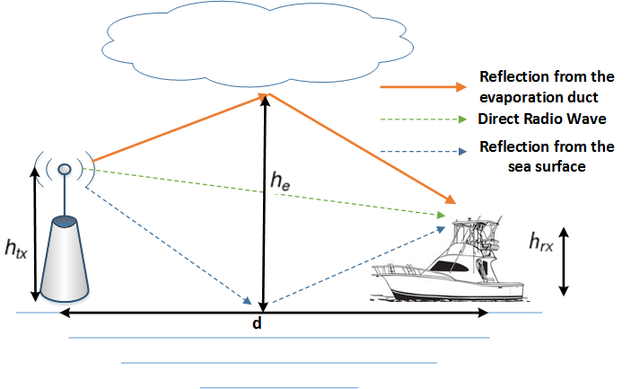
Figure 1: 3-Ray path loss model, where $h_{tx}$ is the height of the transmitter, $h_{rx}$ is the height of receiver, $h_{e}$ is the evaporation duct height and $d$ is the distance between the transmitter and receiver.

Now, the radio resource allocation problem in LTE networks has been also an extensive research topic for long [9, 10]. It begins from a small resource block called Radio resource block (RB) that is assigned to a user [11] to cater its service demand that can range from few kilobits per second (Kbps) to some megabits per second (Mbps).

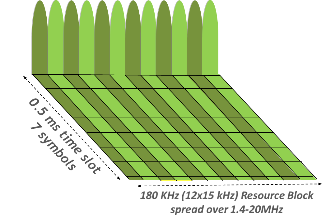
Figure 2: A radio resource block.

A RB has 12 orthogonal frequency division multiplexing (OFDM) subcarriers that are adjacent to each other with a spacing of 15 kHz between two adjacent subcarriers. Each RB (Fig. 2) consists of two sub-time slots of 0.5 ms and each of these sub-time slot utilizes 6 OFDM symbols when normal cyclic prefix is used and 7 OFDM symbols when extended cyclic prefix is used. In RB assignment, the channel state information plays a vital role [12] and this information is acquired by an eNodeB from its connected users periodically. Based on this information, an eNodeB decides upon the modulation and coding scheme (MCS) [13] and the number of radio blocks that it needs to allocate to its connected users. However, in LTE downlink, if a user has been assigned to more than one RB, all these RBs must have the same MCS. This increases the complexity of the radio resource allocation problem.
In this study, the max-min optimization technique that is used extensively in wifi optimization [14, 15] is leveraged for marine channels. However, some early research on resource block optimization that used the max-min approach relied on the characteristics of the urban channels and hence have a different settings than this study [12, 16]. To our best knowledge, no studies have been performed for LTE resource allocation over the sea channels. Hence, this much needed work fills the gap for such case. The rest of the paper is organized as follows: In Section II, we define the LTE-SINR path loss modelling in sea environment. In Section III, we introduce LTE system parameters and the problem formulation. Section IV presents the simulation results and discussions. Lastly, the final conclusion and future work are given in Section V.

Table I: MCS (Modulation and Coding Schemes), SINR, and MCS Efficiency.

MCS	Modulation	Code Rate	SINR Threshold [dB]	Efficiency [bits/symbol]
MCS1	QPSK	1/12	-6.5	0.15
MCS2	QPSK	1/9	-4	0.23
MCS3	QPSK	1/6	-2.6	0.38
MCS4	QPSK	1/3	-1	0.60
MCS5	QPSK	1/2	1	0.88
MCS6	QPSK	3/5	3	1.18
MCS7	16QAM	1/3	6.6	1.48
MCS8	16QAM	1/2	10	1.91
MCS9	16QAM	3/5	11.4	2.41
MCS10	64QAM	1/2	11.8	2.73
MCS11	64QAM	1/2	13	3.32
MCS12	64QAM	3/5	13.8	3.90
MCS13	64QAM	3/4	15.6	4.52
MCS14	64QAM	5/6	16.8	5.12
MCS15	64QAM	11/12	17.6	5.55

II LTE-SINR path loss Modelling in Sea Environment

In this section, we will describe the important consideration for path loss modelling in sea environment. Simulations results as seen in Fig. 3 show that the received signal over distances in the case of 3-Ray path loss model is not as flat when compared to 2-Ray path loss model. It is because of the signals that are received at the receiver by reflections from the sea surface and the evaporation duct. Although, modified 2-Ray model resembles the 3-Ray model but for LTE over sea, a better estimate of the received signal power is determined by 3-Ray path loss model as it gives near to practical results [8]. Mathematically, the 2-Ray path loss propagation model, 2-Ray modified path loss propagation model, and 3-Ray path loss propagation model [8] can be represented as:

$$L_{2-Ray}=-10log_{10}\left(\frac{(h_{tx}\cdot h_{rx})^{2}}{d^{4}\cdot I}\right)$$

$$L_{2-RayMod.}=-10log_{10}\left(\left(\frac{\lambda}{4\pi d}\right)^{2}\left({2\sin\frac{2\pi h_{tx}h_{rx}}{\lambda d}}\right)^{2}\right)$$

$$L_{3-Ray}=-10log_{10}\left(\left(\frac{\lambda}{4\pi d}\right)^{2}\times\left({2(1+\triangle})\right)^{2}\right)$$

with

$$\triangle=2\sin\left(\frac{2\pi h_{tx}h_{rx}}{\lambda d}\right)\times\sin\left(\frac{2\pi(h_{tx}-h_{e})(h_{e}-h_{rx})}{\lambda d}\right)$$

with the parameters being

$\lambda$    : Wavelength in meters
$h_{tx}$  : Height of transmitter in meters
$h_{rx}$  : Height of receiver in meters
$h_{e}$   : Height of evaporation duct
$I$    : System loss parameter
$d$    : Distance between transmitting and receiving
              stations.

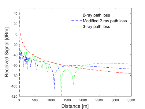
Figure 3: Simulations for different path loss models for sea channels.

For simplicity, in this study we have assumed $h_{e}$ to be around 25 meters. As for our network scenario, we selected two ferry ports: Uskudar and Eminonu in Istanbul, Turkey. Fig. 4 shows these ferry ports on Google Maps™   with assumed ship and eNodeB positions. The distance between these two ports is around 3.7 km and the distance between the two base stations on each port is around 500 meters. At any given moment, there are around 4 to 12 ships travelling from one ferry port to the other. The two lanes ”Eminonu to Uskudar” and ”Uskudar to Eminonu” are separated by around 300-400 meters. To represent ships, aka users, we choose equidistant points in the sea lane, and to represent eNodeB’s we fixed 4 points on the land just near to the ports. The ship distances are assumed uniform in the sea.

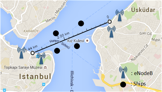
Figure 4: Eminonu and Uskudar ferry ports as seen on Google Maps^TM with assumed ships and eNodeB positions.

III LTE system parameters and the problem formulation

In this section, we define all the assumptions and the LTE system parameters that are required to describe the radio resource allocation problem. Problem formulation with different radio resource allocation methods and their solution are also described in detail in this section.

III-A Assumptions

The two basic fundamental assumptions [17] regarding our allocation method are : a) Throughput perceived by any user $j$ from the connected eNodeB $i$ is a function of how many resource element has been allocated rather than what those resources are, b) Throughput increases strictly for a user if more resources are allocated to it.
Denoting $\beta_{j}$ as a normalised ratio of resource assigned from an eNodeB $i$ to a user $j$ with $\beta_{i}\in[0,1]$, we have

$$\beta_{j}\overset{\Delta}{=}\frac{r_{ij}}{s_{i}}$$

where $r_{ij}$ are the resources allocated by an eNodeB $i$ to a user $j$ and $s_{i}$ are the total available resources with the eNodeB $i$. Thus, the throughput $(T_{j})$ can be written as a strictly increasing function of $\beta$ as:

$$T_{j}=g_{j}(\beta_{j}).$$

The assumptions described earlier takes care of orthogonal resource allocation and channel state information availability. Also, it can be intuitively deduced that the throughput would be maximum, if

$$\sum_{j=0}^{J}\beta_{j}=\sum_{j=0}^{J}\psi_{j}\left(T_{j}\right)=1$$

where

$$\psi_{j}(T_{j})\overset{\Delta}{=}g_{j}^{-1}.$$

Now, we will define the LTE system parameters.

III-B LTE system parameters:

The LTE system parameters involved in the problem formulation are described as follows:

• $user\ j=1,2,3,....,J;$ where a user represents a ship in our case.

• $eNodeB\ i=1,2,3,....,I;$

• $n=1,2,3,....,N;$ where $n$ is the number of resource blocks.

• $SINR\ calculation\ parameters$ : For a user $j$ that is connected to an eNodeB $i$, the SINR can be given by:
  

  $$SINR_{i,j}=\frac{Power_{i,j}\cdot\Gamma_{i,j}}{\sum_{m=1,m\neq i}^{I}Power_{m,j}\cdot\Gamma_{m,j}+\sigma^{2}}$$

  where $\Gamma_{i,j}$ is the channel gain between eNodeB $i$ and user $j$, and $\sigma^{2}$ is the zero mean noise variance. This $SINR$ represents the link conditions and is used to determine the connection and throughput between a user and an eNodeB.

• $Throughput\ space\ matrix$ : We represent the throughput space matrix as:

  $$Th\left[I\right]\left[J\right]=\bar{T}_{ij}.\ \forall i\in[1,I],j\in[1,J]$$

  The throughput space matrix entries ($\bar{T}_{ij}$’s) is defined as throughput per RB between the user $j$ and eNodeB $i$ and is calculated on the basis of MCS values with respect to SINR levels [12, 13] as given in Table I. The demand per user is represented as :
  

  $$D_{j}=\phi$$

  where $\phi$ is the minimum best throughput that can be guaranteed to a user in the network.

Finally, Table II summarizes LTE system parameters that were used in the simulations. Since we are utilizing 2x2 MIMO, we assume that the data rate is doubled as compared to the data rate of a single antenna mode. Lastly, for the sake of simplicity the noise variance is taken as 1.

Table II: Simulation Parameters

Parameters	Values
Carrier Frequency	2750 MHz
Number of RBs per eNodeB	25
OFDM data symbol per sub time slot	7
Antenna	2x2 MIMO
eNodeB Tx power	43 dBm
Height of Tx	20 meter
Height of Rx	3 meter
Height of Evaporation Duct	25 meter
Cable loss	3 dBm
Antenna Pattern	Omnidirectional
Carriers per RB	12
Noise Variance	1

III-C Problem formulation:

Given all these assumptions and system parameters, we now describe the problem formulation of the different radio resource allocation methods.

III-C1 Max-min problem formulation

As a starting point, we assume that the users are in the transmission range of all eNodeB’s and can connect to any one of those eNodeB. Also, it is assumed that all the eNodeB’s having perfect knowledge of channel state information and thus, have the knowledge of throughput space matrix. The max-min method is formulated in such a way that it tries to allocates RBs to the worst throughput links first rather than the better throughput links. This in turn maximizes the minimum throughput of the links in the network and thereby, increases fairness in radio resource allocation. The objective function can be written as Eq. 1 or can be better simplified in two step as Eq. 2 and Eq. 3. Also, initially the demand is assumed to be relaxed that is $\phi=0$ .

$$\max\min_{i\in I}\hskip 5.69046pt\arg\left(\sum_{i=1}^{I}(\bar{T}_{ij}\times K_{ij})\right)\hskip 14.22636pt\forall\ j\in[1,J]$$ (1)

$$Maximize\ (\phi)$$ (2)

$${\sum_{i=1}^{I}\left(\bar{T}_{ij}\times K_{ij}\right)\geq\phi,\hskip 14.22636pt\forall\ j\in[1,J]}$$ (3)

The constraint space is given by:

$$Y_{ij}\in\{0,1\}$$ (4)

$$\sum_{j=1}^{J}K_{ij}\leq N,\hskip 14.22636pt\forall\ i\in[1,I]$$ (5)

$$\sum_{i=1}^{I}Y_{ij}=1,\hskip 14.22636pt\forall\ j\in[1,J]$$ (6)

$$K_{ij}=Y_{ij}\times N,\hskip 14.22636pt\forall\ i,j$$ (7)

$$K_{ij}\geq(D_{j}/\bar{T}_{ij})\times Y_{ij}.\hskip 14.22636pt\forall\ i,j$$ (8)

Eq. (4) defines a binary decision variable $Y_{ij}$ to denote a connection between an eNodeB and a user. Also, an integer decision variable, $K_{ij}$, is defined to signify the number of RBs that can be allocated from an eNodeB $i$ to a user $j$ in the network. Eq. (5) gives a constraint that the maximum RBs that can be allocated to users from a given eNodeB can be $N$. In Eq. (6), $\left({\sum_{i=1}^{I}Y_{ij}}\right)$ is 1 if an eNodeB $i$ is connected to a user $j$, else it is zero. On the other hand, Eq. (7) makes sure that the RBs ($K_{ij}$) are allocated to the only defined connection ($Y_{ij}$). Finally, Eq. (8) gives the capacity constraint with respect to the demand $D_{j}$.
In addition to this formulation, Karush-Kuhn-Tucker (KKT) conditions [18], which are detailed for such problems in [17, 19], holds a strong duality. Therefore, the solution attained in primal form is equal to the dual form. Hence, a near to an optimum resource allocation can be attained while keeping SINR or BER conditions in consideration.

III-C2 Round Robin Method

The round robin allocation method is formulated in such a way that the same amount of resources are given to all users. In this scenario, a user $j$ perceives the throughput proportional to the one that is possible using all resources [17]. Therefore for a user $j$ , the throughput $\bar{T}_{ij}$ is given by :

$$\bar{T}_{ij}=\frac{\sum_{j\in J}\tilde{T_{j}}}{J}\hskip 14.22636pt\forall j\ \in[1,J],$$ (9)

where $J$ is the total number of users in the network and $\tilde{T_{j}}$ is the throughput for the $j^{th}$ user. To simulate such scenarios, we assume that once a connection is established between an eNodeB and its users, the resources are divided equally among them considering the constraint space of limited SINR.

III-C3 Opportunistic method

For the opportunistic case, we formulate the problem as a maximization problem [17] in such a manner that each eNodeB allocates maximum RBs to a high throughput link as compared to low throughput links, thus increasing the network throughput non uniformly among users. In the problem formulation, however, the constraint space will remain the same as the max-min method described earlier.

$$\max_{i\in I}\hskip 5.69046pt\arg\left(\sum_{i=1}^{I}\left(\bar{T}_{ij}\times K_{ij}\right)\right)\hskip 14.22636pt\forall j\ \in[1,J]$$

$$Y_{ij}\in\{0,1\}$$

$$\sum_{j=1}^{J}K_{ij}\leq N,\hskip 14.22636pt\forall\ i\in[1,I]$$

$$\sum_{i=1}^{I}Y_{ij}=1,\hskip 14.22636pt\forall\ j\in[1,J]$$

$$K_{ij}=Y_{ij}\times N,\hskip 14.22636pt\forall\ i,j$$

$$K_{ij}\geq(D_{j}/\bar{T}_{ij})\times Y_{ij}\ \hskip 14.22636pt\forall\ i,j$$

III-D Performance Comparisons

To compare the performance of these methods, we use the very famous Jain index [20], [21]. The Jain index for a user $j$ assuming that it has the throughput $\tilde{T_{j}}$ is given as:

$$F=\frac{\left(\sum_{j\in J}\tilde{T_{j}}\right)^{2}}{N\sum_{j\in J}\tilde{T_{j}}^{2}}\hskip 14.22636pt\forall j\ \in[1,J].$$

In the next section, we detail out the results obtained by these allocation methods with Jain index as an important performance index.

IV Simulation results and discussions

In this section, the results obtained by simulating the models described in above sections are compared and discussed. All these models were simulated in IBM-CPLEX [22]. The simulation environment consisted of a sample network scenario in Bosphorus strait of Istanbul, Turkey (refer to Fig. 4). The four eNodeBs are land based and are placed on the two opposite ferry ports: Eminonu and Uskudar. The ship positions were assumed to be equidistant to each other in the sea lanes between these two ferry ports and the simulations were carried out with different ship densities in the sea that ranged from 4 to 12 ships. The resource allocation fairness index (Table III) thus obtained is plotted in Fig. 5 and it can be seen clearly that the network fairness with different user densities for max-min method is far better than round robin or opportunistic method.
Also, on close analysis of the individual user densities (Figs. 6- 10), it can be concluded that the max-min method guarantees better minimum data throughput per user as compared to the other two methods. This is because the max-min method first allocates RBs to the worst throughput links and then to better throughput links, thus maximizing the minimum throughput of the links in the network. Moreover, the max-min method balances the overall network throughput uniformly with increasing number of the user density than the other two optimization methods.

Table III: Fairness index of different allocation methods with user densities

Number of Users	4	6	8	10	12
Max-Min	0.96	0.85	0.56	0.52	0.94
Opportunistic	0.56	0.37	0.39	0.25	0.26
Round Robin	0.5	0.51	0.59	0.58	0.47

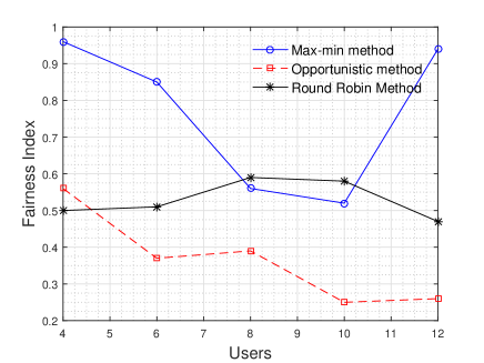
Figure 5: Fairness of algorithms with user density.

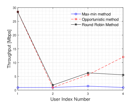
Figure 6: 4 user case: Individual user throughput.

Table IV: A sample 8 user resource block allocation

eNodeB index number	2	2	1	4	4	3	4	3
Connected user index number	1	2	3	4	5	6	7	8
Max-Min Method (RB’s)	2	23	25	12	8	21	5	4
Round Robin Method (RB’s)	13	12	25	8	8	12	9	13
Opportunistic Method (RB’s)	25	1	25	1	1	1	21	25

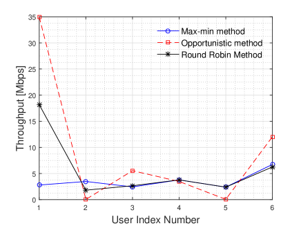
Figure 7: 6 user case: Individual user throughput.

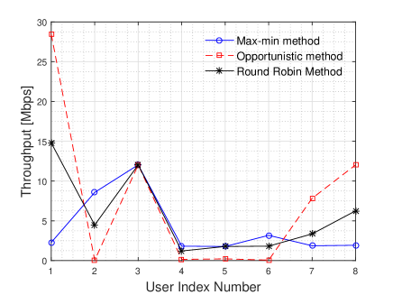
Figure 8: 8 user case: Individual user throughput.

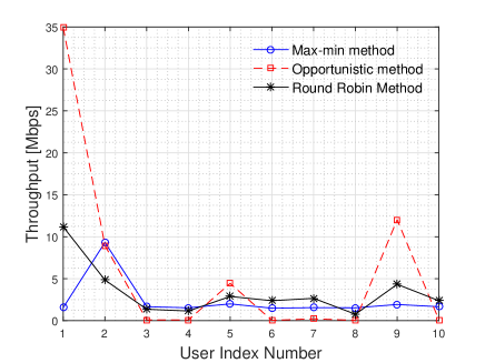
Figure 9: 10 user case: Individual user throughput.

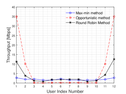
Figure 10: 12 user case: Individual user throughput.

V Conclusion and future work

In this work, we analysed and formulated the radio resource allocation problem by max-min optimization method, which was compared to round robin and opportunistic radio resource block allocation methods. The scenario involved different ship densities at a time. The max-min integer linear programming method results in the minimum best data throughput that can be guaranteed to each and every user in a SINR limited sea channels with a high fairness value than the other two methods. The propagation model used for simulation was 3-Ray path loss as compared to very well known 2-Ray path loss propagation model that is used extensively for urban landscape. Also, it was observed that as the number of users begin to increase, the max-min optimization method performs significantly better with good fairness as compared to the other two methods. In future work, we will look into the joint optimization of power and frequency per sub carrier in LTE network over the sea and also would like to extend the work into the resource allocation problem for 5G networks.

References

- [1] N. Shabbir, M. T. Sadiq, H. Kashif, and R. Ullah, “Comparison of radio propagation models for long term evolution (LTE) network,” arXiv preprint arXiv:1110.1519, 2011.
- [2] Y. Ahmad, W. Hassan, T. A. Rahman et al., “Studying different propagation models for LTE-A system,” in Computer and Communication Engineering (ICCCE), 2012 International Conference on. IEEE, 2012.
- [3] Y. Corre and Y. Lostanlen, “Three-dimensional urban EM wave propagation model for radio network planning and optimization over large areas,” Vehicular Technology, IEEE Transactions on, 2009.
- [4] A. Aragon-Zavala, Antennas and propagation for wireless communication systems. John Wiley & Sons, 2008.
- [5] E. Damosso and L. M. Correia, COST Action 231: Digital Mobile Radio Towards Future Generation Systems: Final Report. European Commission, 1999.
- [6] S. D. Gunashekar, E. M. Warrington, D. R. Siddle, and P. Valtr, “Signal strength variations at 2 GHz for three sea paths in the British Channel Islands: Detailed discussion and propagation modeling,” Radio Science, 2007.
- [7] Q. Lei and M. Rice, “Multipath channel model for over-water aeronautical telemetry,” Aerospace and Electronic Systems, IEEE Transactions on, April 2009.
- [8] Y. H. Lee, F. Dong, and Y. S. Meng, “Near sea-surface mobile radiowave propagation at 5 GHz: measurements and modeling,” Radioengineering, 2014.
- [9] K. Seong, M. Mohseni, and J. M. Cioffi, “Optimal resource allocation for ofdma downlink systems,” in Information Theory, 2006 IEEE International Symposium on. IEEE, 2006, pp. 1394–1398.
- [10] A. Bazzi, G. Pasolini, and O. Andrisano, “Multiradio resource management: Parallel transmission for higher throughput?” EURASIP journal on advances in signal processing, vol. 2008, no. 1, pp. 1–9, 2008.
- [11] A. Ghosh, R. Ratasuk, B. Mondal, N. Mangalvedhe, and T. Thomas, “LTE-advanced: Next-generation wireless broadband technology,” Wireless Commun., 2010.
- [12] D. López-Pérez, A. Ladányi, A. Jüttner, H. Rivano, and J. Zhang, “Optimization method for the joint allocation of modulation schemes, coding rates, resource blocks and power in self-organizing LTE networks,” in INFOCOM, 2011 Proceedings IEEE. IEEE, 2011.
- [13] J. Fan, Q. Yin, G. Li, B. Peng, and X. Zhu, “MCS selection for throughput improvement in downlink LTE systems,” in Computer Communications and Networks (ICCCN), 2011 Proceedings of 20th International Conference on, July 2011.
- [14] A. Kachroo, J. Park, and H. Kim, “Channel assignment with transmission power optimization method for high throughput in multi-access point wlan,” in Wireless Communications and Mobile Computing Conference (IWCMC), 2015 International. IEEE, 2015, pp. 314–319.
- [15] M. Pióro, M. Żotkiewicz, B. Staehle, D. Staehle, and D. Yuan, “On max–min fair flow optimization in wireless mesh networks,” Ad Hoc Networks, vol. 13, pp. 134–152, 2014.
- [16] E. Karipidis, N. Sidiropoulos, and Z.-Q. Luo, “Quality of service and max-min fair transmit beamforming to multiple cochannel multicast groups,” Signal Processing, IEEE Transactions on, vol. 56, no. 3, March 2008.
- [17] F. Zabini, A. Bazzi, and B. Masini, “Throughput versus fairness tradeoff analysis,” in Communications (ICC), 2013 IEEE international conference on. IEEE, 2013.
- [18] S. Boyd and L. Vandenberghe, Convex Optimization. Cambridge University Press, 2004.
- [19] P. Xue, P. Gong, J. H. Park, D. Park, and D. K. Kim, “Max-min fairness based radio resource management in fourth generation heterogeneous networks,” in Communications and Information Technology, 2009. ISCIT 2009. 9th International Symposium on, Sept 2009.
- [20] R. Jain, D.-M. Chiu, and W. R. Hawe, A quantitative measure of fairness and discrimination for resource allocation in shared computer system. Eastern Research Laboratory, Digital Equipment Corporation Hudson, MA, 1984, vol. 38.
- [21] H. T. Cheng and W. Zhuang, “An optimization framework for balancing throughput and fairness in wireless networks with qos support,” Wireless Communications, IEEE Transactions on, vol. 7, no. 2, pp. 584–593, 2008.
- [22] http://www.ibm.com/software/integration/optimization/cplex/.