Kinky plasmons in double layers of borophene-borophene and borophene-graphene

Abstract

We investigate the collective plasmon modes in double layer of two dimensional materials where either one or both of the layers have tilted Dirac cone. Consistent with quite generic hydrodynamic treatment, similar to double layer graphene systems we find two branches of plasmons. The in-phase oscillations of the two layers disperses as $\sqrt{q}$, while the out-of-phase mode disperses as $q$. When even one of the layers hosts tilted Dirac cone spectrum, the plasmonic kink which is a salient feature of a monolayer of tilted Dirac cone is inherited by both of these branches. In double layers composed of graphene (nontilted) and borophene (tilted) where the two layers have two different Fermi velocities, the velocity scale of plasmonic modes is set by the greater of the two. The kink always takes place when each plasmon mode crosses an energy scale $\omega_{\rm kink}$. When the two layers have different chemical potentials, there will be two such scales, and each of in-phase and out-of-phase modes develop two kinks. Moreover we find that an additional linearly dispersing overdamped mode of monolayer tilted Dirac cone system survives in the double layer system.

I Introduction

The concept of two dimensional (2D) Dirac materials began with graphene Novoselov et al. (2004); Kotov et al. (2012); Novoselov et al. (2007); Grigorenko et al. (2012); Novoselov et al. (2004); Castro Neto et al. (2009) which was not only a big step in entering the 2D world but also a playground for 2+1 dimensional quantum field theories. When the Dirac theory comes to condensed matter, it can be deformed in many ways Amorim et al. (2016). One interesting deformation of the Dirac cone is to tilt it Cabra et al. (2013). There are already materials which host tilted 2+1 dimensional Dirac cones. In addition to organic conductor $\alpha$-BEDT Tajima and Kajita (2009); Kobayashi et al. (2009); Katayama et al. (2006); Goerbig et al. (2008); Hirata et al. (2016) which has a weak coupling between layers, a recent example of monolayer borophene Mannix et al. (2015); Cheng et al. (2016); Feng et al. (2017) has also been added to the list of tilted Dirac cone materials. The effect of tilting and anisotropic Fermi velocity on the electronic and collective properties of tilted Dirac cone has been investigated Nishine et al. (2010, 2011); Sári et al. (2014); Proskurin et al. (2015); Verma et al. (2017); Jalali-Mola and Jafari . In Ref. Jalali-Mola and Jafari, , we have obtained an analytic representation of the polarization function for tilted Dirac cone systems from which we have found a kink in the plasmon dispersion. Moreover strong enough tilt gives rise to an additional overdamped plasmon mode which energetically lives in the intraband particle-hole continuum (PHC). The undamped and overdamped plasmon modes at long wavelengths limit have square root and linear dispersion and both of them are depended to the direction of the momentum ${\boldsymbol{q}}$.

Not only the physics of a 2D monolayer borophene as a prototypical tilted Dirac cone material is interesting, but it also possible to think of multilayer of such 2D systems composed of tilted Dirac cones, or combination of tilted and upright Dirac cones. When these layers come close together in a periodic arrangement, situations with potentially new physics can be created. The early investigations of the heterostructure of 2D systems, especially 2D electron gas dates back to the development of molecular beam epitaxy, which was employed to explore macroscopic sample of A-B super lattice like Ga and As compound. Dingle et al. (1980) The simplest of such systems are double layers Jafari (2014). When the layers are far enough to prevent their band overlap, the collective characteristic of the heterostructure of 2D systems will be different from monolayer one. The double layer combination of 2D electron gas in a either uniform dielectric background Chang and Esaki (1980); Das Sarma and Madhukar (1981); Das Sarma and Quinn (1982); Olego et al. (1982); Pinczuk et al. (1986); Santoro and Giuliani (1988); Hwang and Das Sarma (2009); Stauber and Gómez-Santos (2012) or arbitrary dielectric media Profumo et al. (2010, 2012); Gan et al. (2012) forms two plasmon modes corresponding to in-phase and out-of-phase plasmon oscillations of individual layers. The in-phase mode which appears in higher energy, in the long wave length limit disperses as $\omega\sim\sqrt{q}$, while the out-of-phase mode disperses linearly $\omega\sim q$. Indeed the square root behavior of a monolayer follows from a general hydrodynamic treatment, and is independent of macroscopic details Fetter (1973), and holds for every 2D electron gas.

Given that in addition to organic materials a 2D monolayer of borophene hosts tilted Dirac cone, it is timely to consider the double layers of tilted Dirac cone systems. This can be either the double layer of borophene-borophene (DLB) or a double layer of borophene-graphene (DLBG) where the borophene hosts tilted Dirac cone spectrum, while graphene hosts upright Dirac cone. Based on our analytical calculation of the polarization function for tilted Dirac cone Jalali-Mola and Jafari , we will investigate how the kink feature of monolayer tilted Dirac cone shows up in the double layer setting. In the double layer system, the PHC will be union of the PHC of individual layers. We have established (and will further establish) that in monolayer tilted Dirac cone system, there exists a $\omega_{\rm kink}({\boldsymbol{q}},\eta)$ curve at which a kink in the plasmon dispersion appears which is controlled by the tilt parameter $\eta$. In this work, we find that in DLB systems when the dopings in two layers are different, there will be two such scales, and therefore the number of kinks in each of the in-phase and out-of-phase modes will be doubled. More interestingly in the DLBG system, although the graphene layer does not have a kink in the decoupled limit, as a result of coupling by Coulomb forces to the borophene layer, both resulting plasmon modes will develop a kink at the $\omega_{\rm kink}$ energy scale. Another feature of monolayer tilted Dirac cone system is the presence of an additional plasmon mode which disperses linearly and is heavily damped. We show that in DLB system there is only one such mode, implying that the in-phase overdamped plasmons survive in DLB, while the out-of-phase mode does not exist.

This paper is organized as follows. In section II we give a brief introduction double layer dielectric function and represent the tilted Dirac cone Hamiltonian. Then we analytically study the plasmon modes in the long wavelength limit. In section III we investigate the role of distance, tilting and doping in DLB. In section IV, the plasmon modes are studied in double layer of borophene-graphene. Section V deals with the additional overdamped plasmon branch. The paper ends with a summary in section VI.

II Formulation of plasmons in DLB

To describe the collective excitations of the borophene layers in our double layer system, we need the linear response function of charge density to the external potential and the dielectric function for the double layer system. To begin, the Hamiltonian for DLB which are separated along $z$ direction and are interacting via the long range Coulomb interacton Das Sarma and Quinn (1982); Hwang and Das Sarma (2009)

$$H= \sum_{l,\sigma,{\boldsymbol{k}}}\psi^{{\dagger}}_{{\boldsymbol{k}},\sigma,l}h({\boldsymbol{k}})\psi_{{\boldsymbol{k}},\sigma,l}+$$

$$\frac{1}{2A}\sum_{l,l^{\prime},\sigma,\sigma^{\prime},{\boldsymbol{p}},{\boldsymbol{q}},{\boldsymbol{k}}}V_{ll^{\prime}}({\boldsymbol{q}})\psi^{{\dagger}}_{{\boldsymbol{p}}+{\boldsymbol{q}},\sigma,l}\psi^{{\dagger}}_{{\boldsymbol{k}}-{\boldsymbol{q}},\sigma^{\prime},l^{\prime}}\psi_{{\boldsymbol{k}},\sigma^{\prime},l^{\prime}}\psi_{{\boldsymbol{p}},\sigma,l},$$

where, $h({\boldsymbol{k}})$ is the Hamiltonian for tilted Dirac cone, $l,l^{\prime}=1,2$ are layer indices, and $V_{ll^{\prime}}$ denotes the interlayer ($l\neq l^{\prime}$) and intralayer ($l=l^{\prime}$) Coulomb matrix element. The operator $\psi_{{\boldsymbol{p}},\sigma,l}$ anihilates an electron at Bloch state ${\boldsymbol{p}}$, with $\sigma$ in layer $l$ of area $A$. The tilted Dirac Hamiltonian which describes the low energy electronic properties of borophene and organic conductors (under high pressure) is given by Sári et al. (2014); Suzumura et al. (2014); Tajima and Kajita (2009),

$$h^{R/L}({\boldsymbol{k}})=\pm\hbar\begin{pmatrix}v_{x0}k_{x}+v_{y0}k_{y}&v_{x}k_{x}\mp iv_{y}k_{y}\\ v_{x}k_{x}\pm iv_{y}k_{y}&v_{x0}k_{x}+v_{y0}k_{y}\end{pmatrix}.$$ (2)

Here, L (R) stands for left (right) valley, the diagonal Fermi velocities $v_{x0},v_{y0}$ represent the tilt of the Dirac cone and the off-diagonal Fermi velocities $v_{x}\neq v_{y}$ represent the anisotropic of the principal Fermi velocity. As a special case of Eq. (2), if we assume that the diagonal Fermi velocity is zero and off-diagonal Fermi velocities are equal (symmetric), it will reduce to the graphene case. The noninteracting single-particle energy and eigenstates of tilted Dirac fermions after affecting a transformation on Cartesian coordinate $k_{x},k_{y}$, are given by

$$E^{R/L}_{\lambda}({\boldsymbol{k}})=\pm\hbar v_{x}(\eta k_{x}+\lambda k),$$

$$\ket{{\boldsymbol{k}},\lambda}^{R}=\frac{1}{\sqrt{2}}\begin{pmatrix}1\\ \lambda e^{i\theta_{k}}\end{pmatrix},\leavevmode\nobreak\ \leavevmode\nobreak\ \leavevmode\nobreak\ \ket{{\boldsymbol{k}},\lambda}^{L}=\frac{1}{\sqrt{2}}\begin{pmatrix}1\\ -\lambda e^{-i\theta_{k}}\end{pmatrix},$$ (3)

where $\lambda=\pm$ and the tilt parameter $\eta$ is defined as

$$\eta=\sqrt{\frac{v_{x0}^{2}}{v_{x}^{2}}+\frac{v_{y0}^{2}}{v_{y}^{2}}}.$$ (4)

The intralayer and interlayer Coulomb interaction for the pair parallel of 2D borophene layer in a medium with different dielectric constant around ($\epsilon_{1},\epsilon_{d},\epsilon_{2}$ form top to bottom) is given byProfumo et al. (2010)

$$V_{11}=\frac{4\pi e^{2}}{qD(q)}\bigg{(}(\epsilon_{d}+\epsilon_{2})e^{qd}+(\epsilon_{d}-\epsilon_{2})e^{-qd}\bigg{)},$$

$$V_{21}=V_{12}=\frac{8\pi e^{2}}{qD(q)}(\epsilon_{d}),$$ (5)

where,

$$D(q)=(\epsilon_{1}+\epsilon_{d})(\epsilon_{d}+\epsilon_{2})e^{qd}+(\epsilon_{1}-\epsilon_{d})(\epsilon_{d}-\epsilon_{2})e^{-qd}.$$ (6)

Here, it has been assumed that the first (second) layer, $l=1$ ($l=2$), is located at $z=d$ ($0$) and has been sandwiched between two dielectric media $\epsilon_{1}$ at the top and $\epsilon_{d}$ ($\epsilon_{d}$ and $\epsilon_{2}$ at the bottom). Hence, $V_{22}$ can be find thorough $V_{11}$ by changing variable $\epsilon_{2}\to\epsilon_{1}$.

Within the random phase approximation (RPA), and ignoring the interlayer PH propagators, the dressed density response function can be expressed as Das Sarma and Madhukar (1981); Hwang and Das Sarma (2009); Das Sarma and Quinn (1982); Santoro and Giuliani (1988)

$$\chi({\boldsymbol{q}},\omega)=\chi_{0}({\boldsymbol{q}},\omega)\mathbb{1}-\boldsymbol{V}(q),$$ (7)

with $\boldsymbol{V}(q)$ as electron-electron interaction matrix (in the space of layer indices) and $\chi_{0}$ as noninteracting density response function in which as long as the band overlap between layers is absent, the off diagonal (interlayer) density response tensor element is zero, and therefor a unit matrix on the right hand side multiplies the scalar $\chi_{0}$. The dielectric function derived from Eq. (7) is given by the matrix equation

$$\boldsymbol{\varepsilon}({\boldsymbol{q}},\omega)=\mathbb{1}-\chi_{0}({\boldsymbol{q}},\omega)\boldsymbol{V}(q).$$ (8)

Now the dispersion of collective excitations is obtained by

$$\det\boldsymbol{\varepsilon}({\boldsymbol{q}},\omega)=0.$$ (9)

To begin investigating the plasmon mode properties in the DLB we first analyze the density response and its plasmons in long wavelength limit, analytically. Using linear response theory, the density fluctuation of the noninteracting borophene monolayer in the presence of external electromagnetic filed is given by,

$$\chi_{0}(\boldsymbol{q},\omega)=$$ (10)

$$\frac{g\gamma^{2}}{A}\sum_{{\boldsymbol{k}},\lambda,\lambda^{\prime}=\pm}\frac{n_{{\boldsymbol{k}},\lambda}-n_{{\boldsymbol{k}}^{\prime},\lambda^{\prime}}}{\hbar\omega+E_{{\boldsymbol{k}},\lambda}-E_{{\boldsymbol{k}}^{\prime},\lambda^{\prime}}+i0^{+}}f_{\lambda,\lambda^{\prime}}({\boldsymbol{k}},{\boldsymbol{k}}^{\prime}),$$

where ${\boldsymbol{k}}^{\prime}={\boldsymbol{k}}+{\boldsymbol{q}}$, $n_{{\boldsymbol{k}},\lambda}$ is Fermi distribution function with $\lambda$ as band index, the factor $\gamma^{2}=v_{x}/v_{y}$ is Jacobian transformation, $g$ includes spin degeneracy, $A$ is area of system and the form factor $f_{\lambda,\lambda^{\prime}}({\boldsymbol{k}},{\boldsymbol{k}}^{\prime})$ is defined as an expectation value of the density operator $\sigma_{0}=\mathbb{1}$ between two eigenstates $\ket{{\boldsymbol{k}},\lambda}$, $\ket{{\boldsymbol{k}}^{\prime},\lambda^{\prime}}$ of the tilted Dirac cone, which is given by

$$f_{\lambda,\lambda^{\prime}}({\boldsymbol{k}},{\boldsymbol{k}}^{\prime})=\bra{{\boldsymbol{k}},\lambda}\ket{{\boldsymbol{k}}^{\prime},\lambda^{\prime}}=\frac{1}{2}(1+\lambda\lambda^{\prime}\cos(\theta_{\boldsymbol{k}}-\theta_{{\boldsymbol{k}}^{\prime}})),$$ (11)

where $\theta_{{\boldsymbol{k}}}$ is a direction of momentum ${\boldsymbol{k}}$ to $x$ axis.

Here we just consider contribution of one valley (say right) in each layer and ignore the effect of intervalley process, which require large momentum transfer. The analytical result of noninteracting density response function has been calculated in Ref. Jalali-Mola and Jafari, by the present authors. In the long wavelength limit $q\to 0$ this result can be summarized as,

$$\chi_{0}(q\rightarrow 0,\omega)\approx\begin{cases}\frac{\mu q^{2}}{4\pi\omega^{2}}F(\eta)&\eta\ll q\leavevmode\nobreak\ \leavevmode\nobreak\ ,\leavevmode\nobreak\ \leavevmode\nobreak\ \frac{\omega\eta}{q}\ll 1,\\ \frac{\mu q^{2}}{4\pi\omega^{2}}G(\eta,\phi)&\eta\gg q\leavevmode\nobreak\ \leavevmode\nobreak\ ,\leavevmode\nobreak\ \leavevmode\nobreak\ \frac{\omega\eta}{q}\gg 1,\end{cases}$$ (12)

where,

$$G(\eta,\phi)=\frac{g}{4\pi\hbar^{2}\eta^{2}v_{x}v_{y}}\bigg{(}\cos 2\phi+\frac{\eta^{2}+(\eta^{2}-2)\cos 2\phi}{\sqrt{1-\eta^{2}}}\bigg{)},$$

$$F(\eta)=\frac{g}{4\pi\hbar^{2}v_{x}v_{y}}(1-\frac{2\omega\eta}{q}).$$ (13)

It can be easily seen that the density response function in Eq. (13) depends on the tilting parameter $\eta$, and the direction $\phi$ of wave vector ${\boldsymbol{q}}$. Note that in the limit $\eta\to 0$, the ($\eta\omega/q\ll 1$ piece of the) above density response function reduces to graphene. Furthermore, the collective excitations of monolayer borophene is a function of $\eta$ and ${\boldsymbol{q}}$ and show square root behavior as typical plasmon in 2D material Fetter (1973); Nishine et al. (2010, 2011); Jalali-Mola and Jafari . However, in the DLB layer, the collective modes are different from monolayer. For quite general values of $\epsilon_{1},\epsilon_{d},\epsilon_{d}$, there will be two branches of plasmons for DLB system, one dispersing as $q^{1/2}$ and the other dispersing as $q^{1}$. For simplicity let us assume that $\epsilon_{1}=\epsilon_{d}=\epsilon_{2}$ are a uniform background dielectric constant. Combining the above equations with Eq. (8) to solve the secular equation (9) gives

$$\omega_{+}^{2}\approx\begin{cases}e^{2}q(\mu_{1}+\mu_{2})F(\eta)&\eta\ll q\leavevmode\nobreak\ \leavevmode\nobreak\ ,\leavevmode\nobreak\ \leavevmode\nobreak\ \frac{\omega\eta}{q}\ll 1,\\ e^{2}q(\mu_{1}+\mu_{2})G(\eta,\phi)&\eta\gg q\leavevmode\nobreak\ \leavevmode\nobreak\ ,\leavevmode\nobreak\ \leavevmode\nobreak\ \frac{\omega\eta}{q}\gg 1,\end{cases}$$ (14)

and,

$$\omega_{-}^{2}\approx\begin{cases}2e^{2}q^{2}dF(\eta)/(\mu_{1}+\mu_{2})&\eta\ll q\leavevmode\nobreak\ \leavevmode\nobreak\ ,\leavevmode\nobreak\ \leavevmode\nobreak\ \frac{\omega\eta}{q}\ll 1,\\ 2e^{2}q^{2}dG(\eta,\phi)/(\mu_{1}+\mu_{2})&\eta\gg q\leavevmode\nobreak\ \leavevmode\nobreak\ ,\leavevmode\nobreak\ \leavevmode\nobreak\ \frac{\omega\eta}{q}\gg 1,\end{cases}$$ (15)

The $\omega_{+}\propto\sqrt{q}$ is the in-phase oscillations of charge density in two layers, and therefore conforms to the generic $\sqrt{q}$ hydrodynamic behavior of 2D systems Fetter (1973). The $\omega_{-}$ is the out-of-phase collective oscillations of the density in two layers. Some times the $\omega_{-}$ is referred to as the ”acoustic” plasmon which is misleading. The acoustic modes in phonon systems refer to the in-phase oscillations of the ions in the same unit cell, while here the linearly dispersing plasmon mode corresponds to out-of-phase oscillations. It is interesting to note that the in-phase plasmon mode does not depend on separation $d$ of the two layers, while the out-of-phase (linearly dispersing) is proportional to $\sqrt{d}$, and its energy increases by increasing the separation $d$ of the layers.

Both plasmonic branches depend on the chemical potential of each layer and the linear one is also sensitively dependent on the separation of the layers. Note that up to this point we have assumed that except for the chemical potential, all other parameters of the two layers forming the DLB are the same. In addition, if we consider different dielectric media, the qualitative behavior remains the same, but the two plasmonic branches will disperse at lower energy and the group velocity of acoustic mode will be modified Profumo et al. (2012). In this paper we assume that our double layer system is placed in the medium with a uniform background dielectric constant, i.e. $\epsilon_{1}=\epsilon_{d}=\epsilon_{2}$. Moreover, when studying bilayers composed of graphene and borophene, their Fermi velocities is assumed to be $v_{F}=c/300,c/1000$, respectively, where $c$ is the light velocity. The fine structure constant is $e^{2}/\hbar c=1/137$. We also assume that the Fermi velocity in $x$ and $y$ directions are the same, $v_{x}=v_{y}=v_{F}$. Moreover, the kink feature in which we are interested is best seen for the direction $\phi=\pi/2$ of the momentum ${\boldsymbol{q}}$. So we will report our plots for this direction. energy $\hbar\omega/\mu_{1}$ (momentum $q/k_{F_{1}}$) where the subscript $1$ refers to layer $1$ which is taken as reference in case the corresponding quantities are different from layer $2$, and the vector ${\boldsymbol{q}}$ is along the $y$ direction.

III Borophene-borophene double layer

In this section we consider, the pair of parallel borophene layers which are placed in background dielectric constant ($\epsilon_{1}=\epsilon_{d}=\epsilon_{2}=1$) and separated by a distance $d$ in $z$ direction and investigate the dependence of the two plasmon dispersions on various parameters such as the tilting parameters ($\eta_{1},\eta_{2}$), chemical potentials ($\mu_{1},\mu_{2}$). The background dielectric constant appears as an overall constant that reduces $V({\boldsymbol{q}})$ to which the results are not very sensitive. So we take the background dielectric constant to be $1$. Moreover, all plots will be in the $(\omega,{\boldsymbol{q}})$ space, where the vertical (horizontal) axis is the dimensionless

III.1 Distance and tilt dependence

To begin with, we consider DLB with both layers at the same chemical potential ($\mu_{1}=\mu_{2}$). Since both layers are made of borophene, they have the same tilting parameter. We take the tilt parameter to be $\eta_{1}=\eta_{2}=0.45$ Sári et al. (2014). In Fig. 1, we show how the plasmon modes disperse by increasing their separation in $z$ direction. Here, we have plotted the plasmon mode dispersion along with the loss function $|\imaginary\varepsilon^{-1}({\boldsymbol{q}},\omega)|$ to clearly show the damping structure. We have assumed in all panels of Fig. 1 that the direction of ${\boldsymbol{q}}$ is fixed by $\phi=\pi/2$. The separation between the two borophene layers in each panel is: (a) $k_{F_{1}}d=0.35$, (b) $k_{F_{1}}d=1.8$, (c) $k_{F_{1}}d=5.3$ and (d) $k_{F_{1}}d=8.9$. In this figure, the in-phase (out-of-phase) plasmon mode i.e. $\omega_{+}$ ($\omega_{-}$) has been shown with purple (black) curves. The red line denotes the plasmon mode for the monolayer borophene. When the separation becomes infinitely large, the two layers are expected to be decoupled, and therefore the in-phase and out-of-phase modes both become degenerate with the monolayer (red) mode. The boundary of interband and intraband PHC which is defined by $\omega_{\rm kink}$ and $\omega_{s}$ has been shown with dotdashed curve and line, respectively. These boundaries are given by Nishine et al. (2010); Jalali-Mola and Jafari

$$\omega_{\rm kink}({\boldsymbol{q}},\eta)=v_{F}q\eta\cos\phi+\frac{2\mu}{1-\eta^{2}}$$ (16)

$$-\sqrt{(v_{F}q)^{2}+\frac{4v_{F}q\mu\eta\cos\phi}{1-\eta^{2}}+\left(\frac{2\mu\eta}{1-\eta^{2}}\right)^{2}}$$

$$\omega_{s}=v_{F}q(1+\eta\cos\phi)$$ (17)

The reason the lower boundary of inter-band PHC is given the name $\omega_{\rm kink}$ is that in Ref. Jalali-Mola and Jafari, we established that at this boundary the plasmon dispersion of a single-layer tilted Dirac cone system develops a kink.

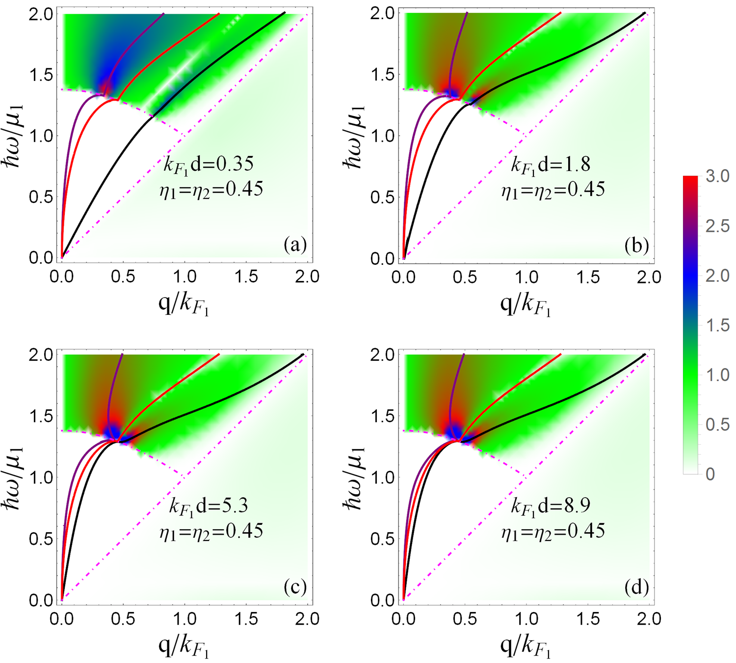
Figure 1: (Color online) Plasmon mode dispersions in DLB system with the same chemical potential ($\mu_{1}=\mu_{2}$) and same tilting parameter ($\eta_{1}=\eta_{2}=0.45$) accompanied with intensity plot of loss function $|\imaginary\varepsilon^{-1}({\boldsymbol{q}},\omega)|$. Here, the vertical (horizontal) axis is the dimensionless energy $\hbar\omega/\mu_{1}$ (momentum $q/k_{F_{1}}$) and the direction of ${\boldsymbol{q}}$ is fixed by $\phi=\pi/2$. The spacing between layers, in various panels are: (a) $k_{F_{1}}d=.35$, (b) $1.8$, (c) $5.3$, and (d) $8.9$. Purple, black and red solid lines are the in-phase ($\omega_{+}$), out-of-phase ($\omega_{-}$) and monolayer plasmon modes, respectively. The pink dotdashed line and curve are the borders of intra-band ($\omega_{\rm kink}$) and inter-band ($\omega_{s}$) PHC, respectively. See the text for details.

As can be clearly seen in Fig. 1, both in-phase and out-of-phase (linear) plasmon mode in all panels maintains their kink in the double layer system as well. Note that since tilt parameter for both layers is the same, they are both characterized with the same $\omega_{\rm kink}$ curve. That is why the combined system develops its kinks on the same curve. Note that the in-phase mode is always above the single-layer mode, while the out-of-phase mode is always below the single-layer mode. This is consistent with picture of two harmonic oscillators coupled via inter-layer Coulomb forces which then splits the degenerate modes into two, lying above and below the degeneracy limit. Since the coupling between the layers becomes zero in the $d\to\infty$ limit, both curves must tend to the single-layer curve by increasing $d$. This can be clearly seen by looking at the trends from panels (a) to (d). It is very pleasant to notice the distance dependence of linear mode. By increasing the distance of layers, the linear (out-of-phase) mode increases. This is consistent with our analytic result in Eq. (15) which suggests that the linear mode depends on distance as $\sqrt{d}$. Upon entering the interband PHC, both modes acquire damping. The undamped portion of the dispersion relation conforms to intuition and both modes tend to the same monolayer dispersion when the distance becomes very large. However the damped portion of the plasmon dispersions which are inside the interband PHC do not degenerate to the same curve. This feature is similar to the case of double layer graphene Hwang and Das Sarma (2009), which is the special case where $\eta_{1}=\eta_{2}=0$.

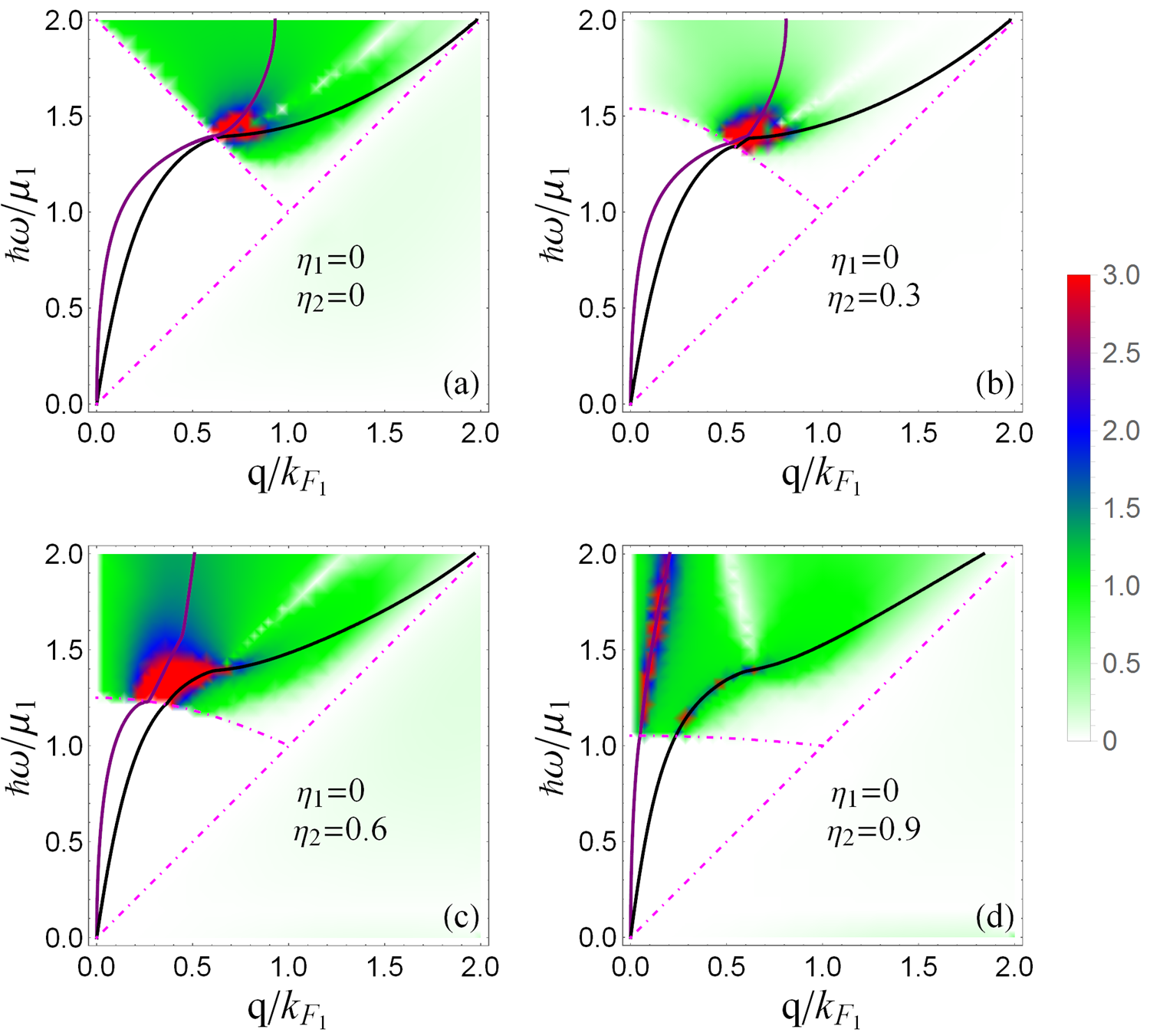
Figure 2: (Color online) Intensity plot of loss function $|\imaginary\varepsilon({\boldsymbol{q}},\omega)|$ and the plasmon dispersions for combination of two tilted Dirac cone layers. The tilt in the first layer is assumed to be zero, i.e. $\eta_{1}=0$, and we vary the tilt strength in the second layer. The direction of ${\boldsymbol{q}}$ is fixed by $\phi=\pi/2$ and the layer spacing is $k_{F_{1}}d=5.3$. The vertical (horizontal) axis is the dimensionless energy $\omega/\mu_{1}$ (momentum $q/k_{F_{1}}$). The tilt parameter $\eta_{2}$ of the second layers is (a) $0$, (b) $0.3$, (c) $0.6$ and (d) $0.9$. Black and purple solid lines are the plasmon modes for $\omega_{+}$ and $\omega_{-}$, respectively. The dotdashed curves are the boundary of PHC as before.

To further investigate the role of tilt parameter, let us assume that one of the layers is not tilted, i.e. $\eta_{1}=0$, and vary the tilt strength $\eta_{2}$ of the other layer. This will teach us how the kink which is the hallmark of tilted Dirac cone evolves in a double layer system. For this purpose in Fig. 2 we plot the plasmon dispersion for ${\boldsymbol{q}}$ in $\phi=\pi/2$ direction. The velocity of both layers are assumed to be identical to that of borophene $\sim c/1000$. In all panels the distance is given by $k_{F_{1}}d=5.3$. The chemical potentials of both layers are also assumed to be the same, so that we only focus on the variation of $\eta_{2}$, as indicated in the legend of each panel. As in the Fig. 1, the in-phase and out-of-phase modes are plotted by purple and black lines and the PHC with dotdashed lines. The separation $d$ of the layers is chosen to be large enough such that the two modes in panel (a) are very close to each other. As can be seen, the effect of tilt in the second layer is to push them away from each other. Furthermore, larger tilt in the second layer increases the energy of the in-phase mode.

Now let us see how the kink is imparted to the two modes. As can be seen from panel (a) in Fig. 2 where both layers have zero tilting there is not kink whatsoever. By increasing $\eta_{2}=0.3,0.6,0.9$ as in panels (b), (c) and (d), both modes develops a kink. This can be intuitively understood as follows: When the layers are decoupled, only the second layer has a kink, as $\eta_{1}=0$. But when they are coupled by Coulomb forces, the in-phase and out-of-phase eigen-modes will be linear combinations of the modes in layers $1$ and $2$. Depending on the relative magnitudes of the coefficients in the linear combination that forms the two eigen modes, the kink will be more manifest in either or both of the symmetric and asymmetric modes. As can be seen in panel (b) for $\eta_{2}=0.3$, the kink in the out-of-phase mode is more manifest, while in panel (c) corresponding to $\eta_{2}=0.6$, the kink for the in-phase mode is more manifest. This observation can be analytically formalized as follows: The eigen-modes for $\eta_{1}=0$ and $\eta_{2}\neq 0$ are given by

$$\omega_{+}^{2}=\frac{e^{2}q\mu}{2}\big{(}F(\eta_{1}=0)+G(\eta_{2},\phi)\big{)},$$

$$\omega_{-}^{2}=e^{2}q^{2}\mu d\frac{F(\eta_{1}=0)G(\eta_{2},\phi)}{F(\eta_{1}=0)+G(\eta_{2},\phi)}.$$ (18)

This is obtained by plugging the long wavelength expression of Eq. (12) in the characteristic equation (9). Note that although this equation is valid in the hydrodynamic limit where $q$ is very small and kinks appear at higher $q$, but still this equation shows how the function $G(\eta_{2},\phi)$ enters both $\omega_{\pm}$ modes. This function encodes information about the kink which is now shared by both $\omega_{\pm}$ modes.

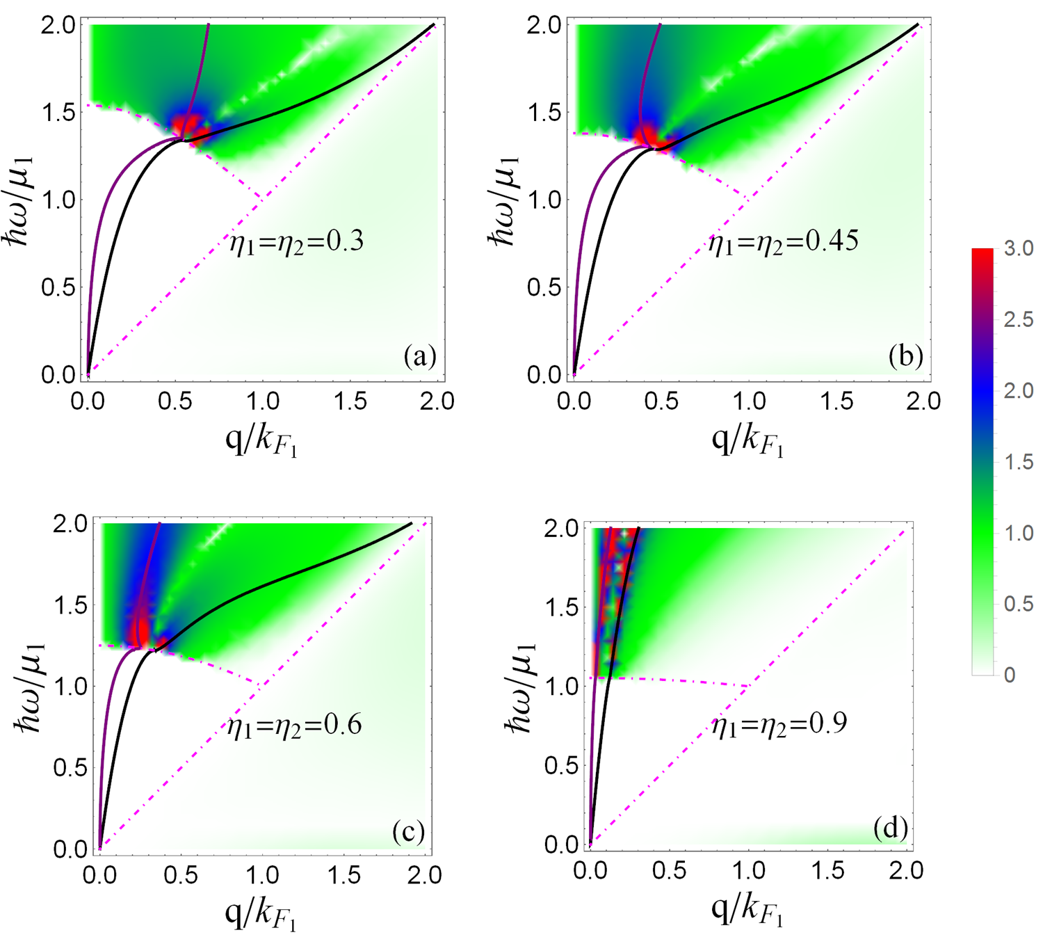
Figure 3: (Color online) The plasmon dispersions for DLB system with equal nonzero tilting parameter($\eta_{1}=\eta_{2}=\eta$) combined with the density plot of loss function $|\imaginary\varepsilon^{-1}({\boldsymbol{q}},\omega)|$. The direction of ${\boldsymbol{q}}$ is fixed by $\phi=\pi/2$ and the layer spacing is $k_{F_{1}}d=5.3$. The vertical (horizontal) axis is the dimensionless quantity $\omega/\mu_{1}$ ($q/k_{F_{1}}$) . The tilting parameter for panel (a), (b), (c), (d) is $\eta=0.3,0.45,0.6,0.9$ respectively. Black and purple solid lines are the plasmon dispersions for $\omega_{+}$ and $\omega_{-}$, respectively. The dotted and Dashed green lines are the boundary of particle hole continuum.

Now let us return to the problem of identically tilted layers. Again both layers have the same chemical potential ($\mu_{1}=\mu_{2}$), the same tilting parameter ($\eta_{1}=\eta_{2}$), and the same velocities. In Fig. 3 we have plotted the symmetric and asymmetric plasmon modes for different tilting parameter. In this figure the tilting parameter of both layers in panels (a), (b), (c) and (d) is given by $\eta_{1}=\eta_{2}=0.3,0.45,0.6,0.9$, respectively. As before, the direction ${\boldsymbol{q}}$ is fixed at $y$ axis. It can be seen that by increasing the tilting parameter from panel (a) to (d), first of all both modes have kinks at $\omega_{\rm kink}$ energy scale. This is intuitive, as both layers have their own kink at $\omega_{\rm kink}$, and so does their both symmetric and asymmetric combinations. Secondly by increasing the kink the splitting between the modes on the $\omega_{\rm kink}$ boundary increases. Third, the dispersions become steeper by increasing the tilt strength. In particular note the very steep dispersion in panel (d) which we have deliberately chosen plot for $\eta_{1}=\eta_{2}=0.9$. This large group velocity can be understood from Eq. (14) and Eq. (15). Both these equations suggest that the plasmon energy depends on $\sqrt{G}$. On the other hand according to Eq. (13), at least near $\eta\sim 1$, the auxiliary function $G$ behaves as

$$G(\eta,\phi)\sim\frac{1-\cos 2\phi}{\sqrt{1-\eta^{2}}}.$$ (19)

This implies that for $\eta\approx 1^{-}$, both in-phase and out-of-phase modes behave like

$$\omega_{\pm}\sim\frac{\sin\phi}{(1-\eta^{2})^{1/4}}\left\{\begin{matrix}q^{1/2}\\ q^{1}\end{matrix}\right.$$ (20)

This singular behavior near $\eta\approx 1$ explains why the plasmon modes become steeper for very large tilting.

To establish the claim of our previous work Jalali-Mola and Jafari that the kink is associated with the energy scale $\omega_{\rm kink}$ of Eq. (17), let us now introduce two such curves corresponding to two different kinks. For this purpose in Fig. 4, we consider DLB with different tilting parameter in each layer. We suppose the first layer has fixed tilting parameter $\eta_{1}=0.45$ and the other layer has a tilt parameter different from $\eta_{1}=0.45$. Panels (a) and (b) of this figure correspond to $\eta_{2}=0.3,0.6$, respectively. Since each $\eta$ according to Eq. (17) gives rise to a distinct boundary $\omega_{\rm kink}$ for the inter-band particle-hole excitations, with two different $\eta_{1}\neq\eta_{2}$ we will have two of them which are plotted as dotdashed lines in Fig. 4. Here again the general trends of plasmon modes are the same as Fig. 2 and Fig. 3. But an important difference is that here as a result of two different tilting parameters of layers, we have two different boundaries given by $\omega_{\rm kink}(\eta_{1})$ and $\omega_{\rm kink}(\eta_{2})$. Now every one of the plasmon branches – either in-phase or out-of-phase modes – develops a kink upon crossing every one of these boundaries. This gives us a total number of four kinks in the plasmon dispersion, two for each mode. Again this can be seen analytically. The eigen modes for arbitrary and nonzero $\eta_{1}$ and $\eta_{2}$ are given by

$$\omega_{+}^{2}=\frac{e^{2}q\mu}{2}\big{(}G(\eta_{1},\phi)+G(\eta_{2},\phi)\big{)},$$

$$\omega_{-}^{2}=e^{2}q^{2}\mu d\frac{G(\eta_{1},\phi)G(\eta_{2},\phi)}{G(\eta_{1},\phi)+G(\eta_{2},\phi)}.$$ (21)

Every $G$ factor contains its own kink information, and therefore both $\omega_{\pm}$ modes will inherit two kinks, one from the $G$ function of each leyer.

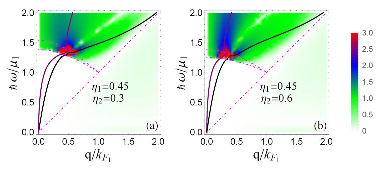
Figure 4: (Color online) Intensity plot of loss function $|\imaginary\varepsilon({\boldsymbol{q}},\omega)|$ and the plasmon dispersions for combination of borophene layers with different nonzero tilting parameter. The direction of ${\boldsymbol{q}}$ is fixed by $\phi=\pi/2$ and the layer spacing is $k_{F_{1}}d=5.3$. The vertical (horizontal) axis is the dimensionless quantity $\omega/\mu_{1}$ ($q/k_{F_{1}}$) . The tilting of the first layer in all panels is $\eta_{1}=0.45$ and the other layer tilting in each panel is, $\eta_{2}=0.3$ in (a) and $0.6$ in (b). Other conventions are the same as previous figures.

III.2 Role of doping

An interesting lesseon can be learned by studying the plasmon modes of two borophene layers where layer $1$ is doped ($\mu_{1}\neq 0$), while the second layer is undoped ($\mu_{2}=0$). When such two layers are infinitely separated, such that the collective charge oscillations in the two layers are decoupled, in layer $1$ we have standard plasmons, while in layer $2$, since the doping level is zero, there are no plasmon oscillations at the RPA level Jalali-Mola and Jafari (2017); Gangadharaiah et al. (2008). Although there will be other types of spin-flip modes Baskaran and Jafari (2002, 2004); Ebrahimkhas and Jafari (2009); Jafari and Baskaran (2012); Tsuchiya et al. (2013); Jafari (2014); Posvyanskiy et al. (2015); Kung et al. (2017) Therefore in terms of counting the collective degrees of freedom, we only have one mode. When the two layers are brought closer at a distance of $k_{F_{1}}d=5.3$ as in Fig. 5 to let them couple, it is not surprising to see that there is only one solution, which clearly corresponds to the $\sqrt{q}$ dispersion. This is a further confirmation that the $\sqrt{q}$ mode is indeed the in-phase mode.

The PHC consist of two contributions. In the doped layer, there is a window below the $\omega_{\rm kink}$. But in the undoped layer, this window is filled with interband PH excitations. Therefore the total PHC which is the union of the PHC for the two layers, consists of no gapped (white) region which will then make the plasmon mode of essentially layer $1$ Landau damped by creasing interband PH excitations in the layer $2$. Indeed we have checked that the dispersion of the present DLB system is almost degenerate with that of a single layer $1$, as long as we are concerned with $\omega<\omega_{\rm kink}$. However, for $\omega>\omega_{\rm kink}$ the plasmon branch enters the interband PHC of layer $1$ itslef, and its dispersion is heavily affected by the presence of layer $2$, and it will no longer be nearly degenerate with the dispersion of a monolayer $1$. Finally note that by increasing the common tilt parameter $\eta_{1}=\eta_{2}$ of the two layers, the energy of the plasmon mode increases. This is a generic behavior in all combinations, as in e.g. Fig. 3.

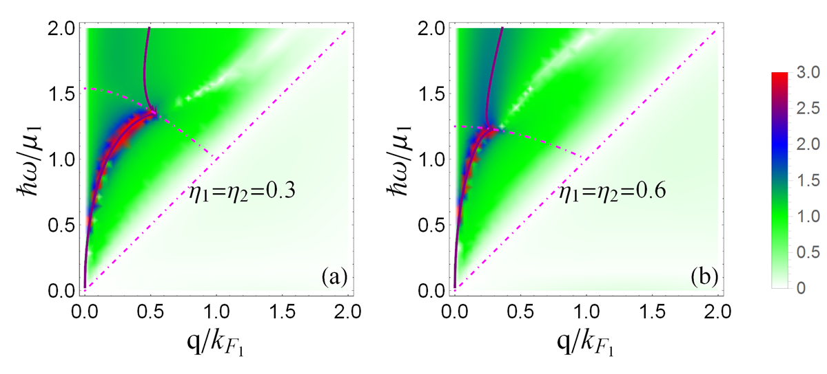
Figure 5: (Color online) The plasmon dispersions for DLB with undoped-doped combination of borophene layer along with intensity plot of loss function $|\imaginary\varepsilon^{-1}({\boldsymbol{q}},\omega)|$ . The vertical (horizontal) axis is the dimensionless energy $\hbar\omega/\mu_{1}$ (momentum $q/k_{F_{1}}$). The direction $\phi$ of ${\boldsymbol{q}}$ in both panels is $\pi/2$. The separation of layers is set by $k_{F_{1}}d=5.3$. The tilting parameter in both layers is the same, $\eta_{1}=\eta_{2}$ which in panel (a) is set to $0.3$, while in panel (b) the tilt parameters are $0.6$. The purple curve is the in-phase. The out-of-phase mode is absent in this case. The pink dotdashed lines are the boundary of interband and intraband PHC. Note that the $\omega_{\rm kink}$ boundary belongs only to the doped layer.

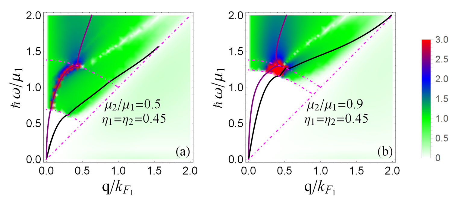
Figure 6: (Color online) The plasmon mode dispersions for DLB system with different chemical potential ($\mu_{1}\neq\mu_{2})$ and same tilting parameter, $\eta_{1}=\eta_{2}=0.45$, and same Fermi velocity. The color code as before indicates the intensity plot of loss function $|\imaginary\varepsilon^{-1}({\boldsymbol{q}},\omega)|$. The vertical (horizontal) axis is the dimensionless energy $\hbar\omega/\mu_{1}$ (momentum $q/k_{F_{1}}$).The separation of layers is set by $k_{F_{1}}d=5.3$. The direction of ${\boldsymbol{q}}$ is fixed in $y$ direction. The doping ratios in panels (a) and (b) are $\mu_{2}/\mu_{1}=0.5$ and $\mu_{2}/\mu_{1}=0.9$, respectively. Black and purple solid lines are the out-of phase and in-phse plasmon modes, respectively. The pink dotdashed lines are the boundary of interband and intraband borophene PHC.

Next, we assume in the DLB we have identically tilted layers with identical velocities, which are doped differently. The difference in doping is quantified by doping ratio. In Fig. 6, we have plotted the plasmon dispersion for DLB system, for the doping ratio $\mu_{2}/\mu_{1}$ given by (a) $0.5$, and (b) $0.9$. The color code is the same as previous figures and the direction of wave vector ${\boldsymbol{q}}$ is fixed in $y$ direction. An important player in this case is the upper border $\omega_{s}$ of the intra-band PHC. As for the border $\omega_{\rm kink}$ of the interband PHC, there will be three possibilities to form the interband particle-hole excitations: (i) within the layer $1$, (ii) within the layer $2$, (iii) cross layer involving particle-hole excitations between layer $1$ and $2$. In the present approximation where interlayer PH propagators are not included, the third item above is absent. The lower bound $\omega_{\rm kink}$ of the intralayer interband for each of the layers are plotted by dottdashed lines. As can be seen first of all, both modes when cross every one of these boundaries, develop a kink. So we end up having two kinks for each mode. Second point to notice is that, in panel (b) where the chemical potentials are closer to each other, the $\omega_{\rm kink}$ boundaries approach to each other. In this case, we have two decent $\omega_{\pm}$ modes. However by reducing the ratio $\mu_{2}/\mu_{1}$, the nearly triangle shaped region shrinks more and more. As a result, the out-of-phase mode (black line) is attracted more and more to the intraband PHC. At the limit $\mu_{2}/\mu_{1}=0$ of Fig. 5, the out-of-phase mode is entirely swallowed by the intraband PHC.

IV Brophene-Graphene

So far we have assumed that both layers are composed of borophene, such that the Fermi velocities are identical. In this section, we are going to study a double layer composed of borophene and graphene. In this case, a new player will be the difference in the Fermi velocity of the two layers. The Fermi velocity sets the slope of the boundary $\omega_{s}$ of the intraband PHC for every layer.

The monolayer graphene as a 2D Dirac material with Fermi velocity $c/300$ and borophene layer as a 2D tilted Dirac material with Fermi velocity $\approx c/1000$ are a good candidate for constructing a double layer system. Another candidate for the tilted Dirac cone layer at the bottom can be organic material Kajita et al. (2014) which has even smaller Fermi velocity. In what follows we consider a double layer of borophene-graphene and study the effect of different Fermi velocity and chemical potential. In this case the two branches of plasmons in the long wave length limit will be given by

$$\omega_{+}^{2}=\frac{e^{2}q\mu}{2}\big{(}F^{(2)}(0)+G^{(1)}(\eta_{1},\phi)\big{)},$$

$$\omega_{-}^{2}=e^{2}q^{2}\mu d\frac{F^{(2)}(0)G^{(1)}(\eta_{1},\phi)}{F^{(2)}(0)+G^{(1)}(\eta_{1},\phi)},$$ (22)

where the superscript in parenthesis indicates their layer indices. More explicitly, $F^{(2)}$ is the same as function $F$ but specialized for layer $2$ whose Fermi velocity is $v_{F_{2}}$. The argument $0$ of this function indicates that the tilt parameter $\eta_{2}=0$ as it stands for graphene layer. Similarly $G^{(1)}$ is the same function $G$ for the layer $1$ whose Fermi velocity is $v_{F_{1}}$, and its tilt is $\eta_{1}$.

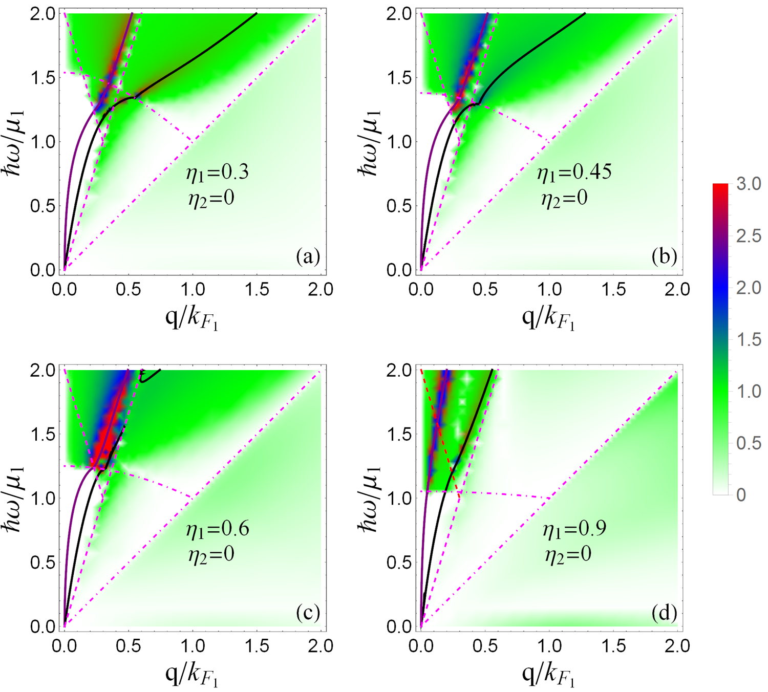
Figure 7: (Color online) Plasmon dispersions in DLBG system along with intensity plot of loss function $|\imaginary\varepsilon^{-1}({\boldsymbol{q}},\omega)|$. The direction of ${\boldsymbol{q}}$ is fixed by $\phi=\pi/2$, the layers separated by $k_{F_{1}}d=5.3$ have same chemical potential ($\mu_{1}=\mu_{2}$) and the tilting parameter of borophene layer (number $1$) in each panel is: (a) $\eta_{1}=0.3$, (b) $\eta_{2}=0.45$ (c) $\eta=0.6$, and (d) $\eta=0.9$. Purple and black solid lines are the plasmon dispersions for $\pm$ modes, respectively. The dotdashed (dashed) pink lines are the boundary of interband and intraband borophene (graphene) PHC. The vertical (horizontal) axis is the dimensionless energy $\hbar\omega/\mu_{1}$ (momentum $q/k_{F_{1}}$). The graphene layer, $2$ has no tilting, $\eta_{2}=0$.

First in Fig. 7 we show the plasmon modes in the DLBG with equal chemical potential ($\mu_{1}=\mu_{2}$) but different Fermi velocity $v_{F_{1}}\neq v_{F_{2}}$. As pointed out, the subscripts $1,2$ stand for borophene and graphene respectively. The tilting parameter for graphene layer, $\eta_{2}=0$ and tilting parameter for borophene layer in panel (a), (b), (c), (d) are taken to be $\eta_{1}=0.3,0.45,0.6,0.9$, respectively. The unit of energy is taken to be $\mu_{1}$ which equals $\mu_{2}$. However, since the Fermi velocities are different, for the unit of momentum one must specify either of the Fermi wave vectors, $k_{F_{1}}$ or $k_{F_{2}}$ as the unit of energy. We adopt the former, and therefore the horizontal axis is the dimensionless momentum $q/k_{F1}$, and the vertical axis (as before) is the dimensionless energy $\omega/\mu_{1}$. The color code is the same as previous figures. The PHC boundary of borophene (graphene) has been defined by dotdashed (dashed) lines Nishine et al. (2010); Jalali-Mola and Jafari . As can be seen from, Fig. 7 the PHC boundary of graphene has the larger slope as a result of its larger Fermi velocity value. Since the plasmons of monolayer of graphene are split off from its intraband PHC, in a combined DLBG system too, the level repulsion from the intraband PHC of graphene pushes both modes to higher energies. This feature not only holds for the undamped portion of the plasmon branches, but it also holds for the damped portion of both branches that enters the interband PHC of the union of interlayer and intralayer PH excitations. So the essential role of the difference in the velocity of the two layers is to sustain both plasmon branches at velocities larger than the greater of the two.

Note that in the DLBG system the PHC will be the union of intralayer PH excitations of both layers. In this way, the interband portion of the PHC for moderate $\eta_{1}$ comes below the $\omega_{\rm kink}$ curve. This is manifest in panels (a), (b) and (c) of Fig. 7 where the dashed boundary (of graphene PHC) has come below the dotdashed boundary (of the borophene PHC). In this way, the damping of $\pm$ modes in panels (a) and (b) start at lower energy and momenta than anticipated from $\omega_{\rm kink}$ curve. Please note that, although the damping might start before the modes hit $\omega_{\rm kink}$ (dotdashed upper boundary), but the kink always starts once the modes cross the $\omega_{\rm kink}$ boundary. This establishes that the $\omega_{\rm kink}$ very well deserves the subscript ”kink”. Finally, again the generic property of both modes can be observe that the energy of both modes increases by increasing the tilt parameter. Note that as argued for Fig. 2, in the decoupled limit, only borophene layer has kinks, while in the coupled graphene-borophene double layer, both dispersions have a kink at $\omega_{\rm kink}$.

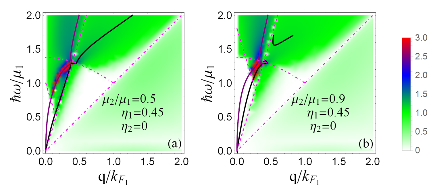
Figure 8: (Color online) Plasmon dispersions in DLBG for different chemical potential together with intensity plot of loss function $|\imaginary\varepsilon^{-1}({\boldsymbol{q}},\omega)|$. The direction of ${\boldsymbol{q}}$ is fixed by $\phi=\pi/2$ and the tilting parameter of borophene layer is $\eta_{1}=0.45$ which is separated by $k_{F_{1}}d=5.3$, where the chemical potential $\mu_{1}$ is fixed and is unit of energy. The chemical $\mu_{2}$ is given by the ratio $\mu_{2}/mu_{1}$ which is (a) $0.5$ and (b) $0.9$. The rest of the conventions are as in Fig. 7.

Next, we consider DLBG with different chemical potential ($\mu_{2}\neq\mu_{1}$) and of course with different Fermi velocities in Fig. 8. In this figure the borophene layer is assumed to have the tilting $\eta_{1}=0.45$ and its chemical potential ($\mu_{1}$) is greater than the chemical potential of graphene ($\mu_{2}$). As can be seen the undamped window for plasmon mode dispersion is more restricted as a result of different chemical potentials. Let us start by panel (b) where chemical potentials are different, but close to each other. In this case both in-phase and out-of-phase modes are present, and their group velocity scale is set by the greater velocity (which belongs to graphene). Decreasing the chemical potential $\mu_{2}$ of graphene, the ”nearly” triangular window which is formed by the union of intralayer PHC of both layers, shrinks and the out-of-phase mode starts to sink into the intraband PHC dominated by PH excitaions of graphene. By further decrease in the $\mu_{2}$, the out-of-phase mode will entirely disappear. This feature is similar to one considered in Fig. 5, where the out-of-phase mode is swallowed by the PHC. In addition, as in all figures, both modes will have their kinks at their intersection with $\omega_{\rm kink}$. Note that in panel (b) of Fig. 8 and panel (c) of Fig. 7 the out-of-phase mode is interrupted. The region of interruption in both cases happens when the intrabanc PHC of graphene hits the plasmon branch. The density of PH excitations in intraband PHC are always much larger than the interband ones, and hence are able to destroy the plasmon branches that hits this portion of PHC.

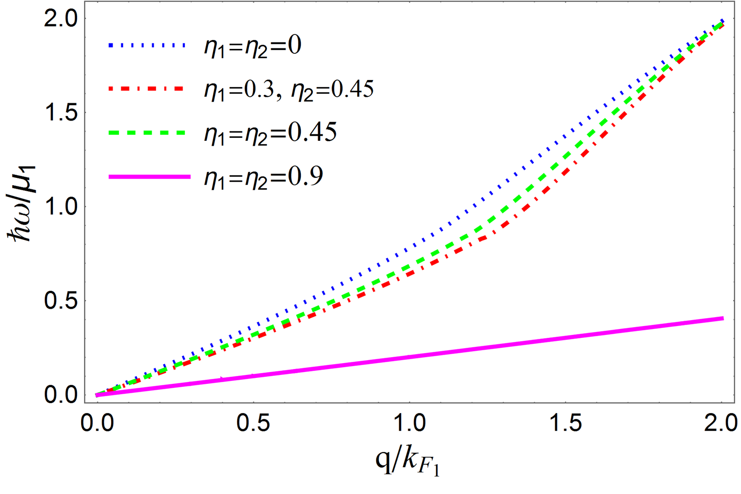
Figure 9: (Color online) Plasmon dispersions in DGL and DLB and with the same chemical potential. The direction of ${\boldsymbol{q}}$ is fixed by $\phi=\pi/2$. Here the tilting parameter for each line is: the blue dotted line points $\eta_{1}=\eta_{2}=0$ for DGL, the green dashed line points $\eta_{1}=0.3,\eta_{2}=0.45$ for DLB, the green dotdashed line points $\eta_{1}=\eta_{2}=0.45$ and the pink solid line points $\eta_{1}=\eta_{2}=0.45$ for DLB. The vertical (horizontal) axis is the dimensionless quantity $\hbar\omega/\mu_{1}$ ($q/k_{F_{1}}$). The separation of layers is set by $k_{F_{1}}d=5.3$.

V Overdamped Plasmon branch

In our previous work Jalali-Mola and Jafari , we noted that an exclusive consequence of the tilt, in addition to kinks in the dispersion of plasmons in monolayer system, is to provide a unique chance for the emergence of an overdamped branch of plasmon excitations which lies deep in the intraband PHC. Since the density of intraband PH excitations is quite large, this provides a significant bath for Landau damping of this plasmon branch, and therefore it gets quickly damped. Although this branch is heavily damped, but since it lives in lower energy than the standard plasmon branch, in time scales smaller than its lifetime $\tau$, it will be able to interact with other low-energy excitations, including the single-particle excitations. Therefore it is important to study this branch in the double layers as well.

In Ref. Jalali-Mola and Jafari, , we found that the overdamped plasmon branch for borophene monolayer is in the energy range $\omega<\omega_{s}$. This mode is caused by strong enough tilt, and disperses linearly. In the case of monolayer graphene where there is no tilt, such an overdamped mode does not exist at all. It is interesting to note that when it comes to double layer graphene, such an overdamped mode will appear. This has not been explored in earlier publications addressing the double layer systems Hwang and Das Sarma (2009); Gan et al. (2012); Profumo et al. (2012). However, we find that even for upright Dirac cones in a double layer system, an overdamped branch emerges. Fig. 9, shows the dispersion of overdamped plasmon for a double layer composed of tilted Dirac cone systems, where Fermi velocities and chemical potentials and are the same. The dispersion has been plotted for $\phi=\pi/2$. The distance is fixed by $k_{F_{1}}d=5.3$. Values of tilt parameter for each layer is indicated in the legend. As can be seen, even for $\eta_{1}=\eta_{2}=0$ there is an overdamped plasmon branch. The effect of tilt in each of layers is to reduce the energy of the overdamped plasmon mode. The solid line represents the overdamped plasmon mode for quite large tilts $\eta_{1}=\eta_{2}=0.9$. This mode disperses linearly over a much larger range of momenta, while for smaller values of tilt parameters, the linear dispersion holds upto $q\sim k_{F_{1}}$. When one of the layers is doped and the other one is undoped, there will be no overdamped solution.

VI Summary and conclusion

In this work, we investigated plasmon oscillations in double layer systems where either one or both of the layers have tilted Dirac cone spectrum. It is well known that in this context, there will be two plasmon modes. The in-phsae mode will disperse as $\sqrt{q}$ – consistent with the hydrodynamic picture – while the out-of-phase mode disperses as $q^{1}$. The in-phase (symmetric) mode always lies at higher energies that the out-of-phase (asymmetric) mode. This is in contrast to the intuition from molecular orbitals where the symmetric combination of atomic orbitals usually has lower energy than the asymmetric combination. This is because in the present case, we are dealing with a symmetric combination of particle-hole objects, and not single-particle orbitals. An extra minus sign coming from the fermion loop places the symmetric plasmons at higher energies.

When the tilted Dirac cone systems are combined in a double layer framework, interesting plasmonic features arises. The tilt of the Dirac cone is manifested in its plasmons as a kink when it crosses $\omega_{\rm kink}$. Such a kink is absent in Dirac cone without tilt. In a bilayer setting we find quite generically that even when one of the layers hosts tilted Dirac cone, the plasmonic kink will be inherited by both in-phase and out-of-phase mode. This kink in both branches takes place at precisely $\omega_{\rm kink}$. In situation such as in Fig. 6 where due to difference in the chemical potential of the two tilted Dirac cone layers there are two $\omega_{\rm kink}$ energy scales, each of the plasmon branches develops a kink upon crossing every $\omega_{\rm kink}$ (dotdashed pink) curve. In this situations there will be a total number of four kinks; two kinks for every plasmon branch.

When one of the layers is graphene with larger Fermi velocity, the small window where undamped plasmons can live will become smaller and will be set by the larger Fermi velocity of graphene. This pushes both in-phase and out-of-phase plasmon modes to higher energy. Therefore the typical plasmonic group velocity in such double layer systems with two different Fermi velocities, is set by the greater of the two velocities.

Another unique feature of tilted Dirac cone monolayer is the existence of linearly dispersing overdamped plasmon mode inside the intraband PHC. Although this mode does not exist in monolayers of upright Dirac cone systems such as graphene, in the double layer setting such a mode emerges. In the double layer systems with tilt, this mode continuously reduces its slope by increasing the tilt. This mode is the in-phase overdampled oscillation of the individual tilted layers Jalali-Mola and Jafari .

References

- Novoselov et al. (2004) K. S. Novoselov, A. K. Geim, S. V. Morozov, D. Jiang, Y. Zhang, S. V. Dubonos, I. V. Grigorieva, and A. A. Firsov, Science 306, 666 (2004).
- Kotov et al. (2012) V. N. Kotov, B. Uchoa, V. M. Pereira, F. Guinea, and A. H. Castro Neto, Rev. Mod. Phys. 84, 1067 (2012).
- Novoselov et al. (2007) K. S. Novoselov, Z. Jiang, Y. Zhang, S. V. Morozov, H. L. Stormer, U. Zeitler, J. C. Maan, G. S. Boebinger, P. Kim, and A. K. Geim, Science 315, 1379 (2007).
- Grigorenko et al. (2012) A. N. Grigorenko, M. Polini, and K. S. Novoselov, Nature Photonics 6, 749 (2012).
- Castro Neto et al. (2009) A. H. Castro Neto, F. Guinea, N. M. R. Peres, K. S. Novoselov, and A. K. Geim, Rev. Mod. Phys. 81, 109 (2009).
- Amorim et al. (2016) B. Amorim, A. Cortijo, F. de Juan, A. Grushin, F. Guinea, A. Guti rrez-Rubio, H. Ochoa, V. Parente, R. Rold n, P. San-Jose, J. Schiefele, M. Sturla, and M. Vozmediano, Physics Reports 617, 1 (2016).
- Cabra et al. (2013) D. C. Cabra, N. E. Grandi, G. A. Silva, and M. B. Sturla, Phys. Rev. B 88, 045126 (2013).
- Tajima and Kajita (2009) N. Tajima and K. Kajita, Science and Technology of Advanced Materials 10, 024308 (2009).
- Kobayashi et al. (2009) A. Kobayashi, S. Katayama, and Y. Suzumura, Science and Technology of Advanced Materials 10, 024309 (2009).
- Katayama et al. (2006) S. Katayama, A. Kobayashi, and Y. Suzumura., J. Phys. Soc. Jpn. 75, 054705 (2006).
- Goerbig et al. (2008) M. O. Goerbig, J.-N. Fuchs, G. Montambaux, and F. Piéchon, Phys. Rev. B 78, 045415 (2008).
- Hirata et al. (2016) M. Hirata, K. Ishikawa, K. Miyagawa, M. Tamura, C. Berthier, D. Basko, A. Kobayashi, G. Matsuno, and K. Kanoda, Nature Communications 7, 12666 (2016).
- Mannix et al. (2015) A. J. Mannix, X.-F. Zhou, B. Kiraly, J. D. Wood, D. Alducin, B. D. Myers, X. Liu, B. L. Fisher, U. Santiago, J. R. Guest, M. J. Yacaman, A. Ponce, A. R. Oganov, M. C. Hersam, and N. P. Guisinger, Science 350, 1513 (2015).
- Cheng et al. (2016) P. Cheng, S. Meng, L. Chen, and K. Wu, Nature Chemistry 8, 563 (2016).
- Feng et al. (2017) B. Feng, O. Sugino, R.-Y. Liu, J. Zhang, R. Yukawa, M. Kawamura, T. Iimori, H. Kim, Y. Hasegawa, H. Li, L. Chen, K. Wu, H. Kumigashira, F. Komori, T.-C. Chiang, S. Meng, and I. Matsuda, Phys. Rev. Lett. 118, 096401 (2017).
- Nishine et al. (2010) T. Nishine, A. Kobayashi, and Y. Suzumura, J. Phys. Soci. Jpn. 79, 114715 (2010).
- Nishine et al. (2011) T. Nishine, A. Kobayashi, and Y. Suzumura, Journal of the Physical Society of Japan 80, 114713 (2011).
- Sári et al. (2014) J. Sári, C. Tőke, and M. O. Goerbig, Phys. Rev. B 90, 155446 (2014).
- Proskurin et al. (2015) I. Proskurin, M. Ogata, and Y. Suzumura, Phys. Rev. B 91, 195413 (2015).
- Verma et al. (2017) S. Verma, A. Mawrie, and T. K. Ghosh, Phys. Rev. B 96, 155418 (2017).
- (21) Z. Jalali-Mola and S. A. Jafari, arXiv:1807.08589 .
- Dingle et al. (1980) R. Dingle, H. St rmer, A. Gossard, and W. Wiegmann, Surface Science 98, 90 (1980).
- Jafari (2014) S. A. Jafari, EPL (Europhysics Letters) 107, 20005 (2014).
- Chang and Esaki (1980) L. Chang and L. Esaki, Surface Science 98, 70 (1980).
- Das Sarma and Madhukar (1981) S. Das Sarma and A. Madhukar, Phys. Rev. B 23, 805 (1981).
- Das Sarma and Quinn (1982) S. Das Sarma and J. J. Quinn, Phys. Rev. B 25, 7603 (1982).
- Olego et al. (1982) D. Olego, A. Pinczuk, A. C. Gossard, and W. Wiegmann, Phys. Rev. B 25, 7867 (1982).
- Pinczuk et al. (1986) A. Pinczuk, M. G. Lamont, and A. C. Gossard, Phys. Rev. Lett. 56, 2092 (1986).
- Santoro and Giuliani (1988) G. E. Santoro and G. F. Giuliani, Phys. Rev. B 37, 937 (1988).
- Hwang and Das Sarma (2009) E. H. Hwang and S. Das Sarma, Phys. Rev. B 80, 205405 (2009).
- Stauber and Gómez-Santos (2012) T. Stauber and G. Gómez-Santos, Phys. Rev. B 85, 075410 (2012).
- Profumo et al. (2010) R. E. V. Profumo, M. Polini, R. Asgari, R. Fazio, and A. H. MacDonald, Phys. Rev. B 82, 085443 (2010).
- Profumo et al. (2012) R. E. V. Profumo, R. Asgari, M. Polini, and A. H. MacDonald, Phys. Rev. B 85, 085443 (2012).
- Gan et al. (2012) C. H. Gan, H. S. Chu, and E. P. Li, Phys. Rev. B 85, 125431 (2012).
- Fetter (1973) A. L. Fetter, Ann. Phys. 81, 367 (1973).
- Suzumura et al. (2014) Y. Suzumura, I. Proskurin, and M. Ogata, Journal of the Physical Society of Japan 83, 094705 (2014).
- Jalali-Mola and Jafari (2017) Z. Jalali-Mola and S. A. Jafari, arXiv , 1705.04575 (2017).
- Gangadharaiah et al. (2008) S. Gangadharaiah, A. M. Farid, and E. G. Mishchenko, Phys. Rev. Lett. 100, 166802 (2008).
- Baskaran and Jafari (2002) G. Baskaran and S. A. Jafari, Phys. Rev. Lett. 89, 016402 (2002).
- Baskaran and Jafari (2004) G. Baskaran and S. A. Jafari, Phys. Rev. Lett. 92, 199702 (2004).
- Ebrahimkhas and Jafari (2009) M. Ebrahimkhas and S. A. Jafari, Phys. Rev. B 79, 205425 (2009).
- Jafari and Baskaran (2012) S. A. Jafari and G. Baskaran, Journal of Physics: Condensed Matter 24, 095601 (2012).
- Tsuchiya et al. (2013) S. Tsuchiya, R. Ganesh, and T. Nikuni, Phys. Rev. B 88, 014527 (2013).
- Posvyanskiy et al. (2015) V. Posvyanskiy, L. Arnarson, and P. Hedeg rd, EPL (Europhysics Letters) 109, 47005 (2015).
- Kung et al. (2017) H.-H. Kung, S. Maiti, X. Wang, S.-W. Cheong, D. L. Maslov, and G. Blumberg, Phys. Rev. Lett. 119, 136802 (2017).
- Kajita et al. (2014) K. Kajita, Y. Nishio, N. Tajima, Y. Suzumura, and A. Kobayashi, J. Phys. Soc. Jpn. 83, 07002 (2014).