FERMILAB-PUB-18-391-APC
Accepted

Micro-bunching for generating tunable narrow-band THz radiation at the FAST photoinjector

Abstract

This paper presents expected THz radiation spectra emitted by micro-bunched electron beams produced using a slit-mask placed within a magnetic chicane in the FAST (Fermilab Accelerator Science and Technology) electron injector at Fermilab. Our purpose is to generate tunable narrow-band THz radiation with a simple scheme in a conventional photo-injector. Using the slit-mask in the chicane, we create a longitudinally micro-bunched beam after the chicane by transversely slicing an energy chirped electron bunch at a location with horizontal dispersion. In this paper, we discuss the theory related to the micro-bunched beam structure, the beam optics, the simulation results of the micro-bunched beam and the bunching factors. Energy radiated at THz frequencies from two sources: coherent transition radiation and from a wiggler is calculated and compared. We also discuss the results of a simple method to observe the micro-bunching on a transverse screen monitor using a skew quadrupole placed in the chicane.

1 Introduction

Accelerator based sources of THz radiation have been proposed and developed at several laboratories worldwide [1, 2, 3, 4, 5, 6, 7, 8, 9, 10, 11, 12, 13, 14]. THz radiation, whose frequency range is from 0.1 THz (wavelength $\lambda=0.3$ mm) to 30 THz ($\lambda=10\,\mu$m), is non-ionizing and has high transmission through non-metallic materials such as clothes, paper, and plastic. Moreover, many materials have characteristic absorption spectra in this THz range. Therefore, THz radiation has been utilized in fundamental research in material, biological, and engineering science. For application to a wider range of fields such as industry, medicine and homeland security, a compact intense narrow-band THz source with tunable frequency is desired.

Schemes to generate narrow-band THz radiation using laser-modulated electron beams have been proposed [15, 16] which require special purpose modulator sections to modulate the laser pulse acting on the electron beam. Here however, we focus on a simple method of generating a micro-bunched beam using standard components of a photo-injector and a slit-mask [17, 18, 19]. The transverse slicing of a bunch by the mask is transformed into the longitudinal plane taking advantage of transverse dispersion at the slit-mask. We use a magnetic chicane consisting of four dipole magnets to either lengthen or shorten an electron bunch but in both cases create a beam with an appropriate comb structure required to generate THz radiation.

We plan to perform the THz generation experiments at the Fermilab Accelerator Science and Technology (FAST) facility electron linac [20, 21]. The final goal is to produce a narrow-band THz wave with a frequency of over 1 THz and demonstrate that this method can provide a tunable narrow-band THz source. The frequency is tuned by choosing the RF phases in the cavities upstream of the chicane. Moreover, intense THz radiation can be generated due to a high bunch repetition rate.

In this paper, we present the theory related to the micro-bunched beam structure and simulation results of the micro-bunched beam, the expected THz spectra using coherent transition radiation (CTR) and a wiggler, as well as a method for observing the micro-bunched beam on a transverse screen monitor. In section 2, the FAST injector and the beam parameters are shown. In section 3, we describe the theory of the energy chirp, the width of the micro-bunches, the lowest frequency generated from the micro-bunched beam, and micro-bunch observation using a skew quadrupole magnet. The beam optics to generate the micro-bunched beam is shown in Section 4. The expected micro-bunched beam structures, and the bunching factors are shown in Section 5. A calculation of the THz radiation energy from CTR and a wiggler is presented in Section 6. The beam distributions after the chicane when a skew quadrupole is turned on for observing the micro-bunching in the transverse plane are shown in Section 7, and conclusions are presented in Section 8.

2 FAST photoinjector

Figure 1 shows the layout of the FAST photoinjector. The injector consists of an RF gun with a normal conducting 1.5 cell cavity, two TESLA style 9-cell superconducting cavities (CC1 and CC2), a magnetic chicane, a vertical dipole magnet for beam extraction, and a beam dump. A molybdenum disk coated with $\mathrm{Cs_{2}Te}$ is used as the cathode, and the RF gun is similar to the one developed for the FLASH facility at DESY [22]. Electron bunches are emitted with a repetition rate of 3 MHz within a macro-pulse that lasts 1 ms. The RF gun and the two superconducting cavities operate at an RF frequency of 1.3 GHz with a repetition rate of 5 Hz. The main machine and beam parameters are shown in Table 1.

Table 1: Relevant beam and machine parameters

Parameter	Value
Beam energy after gun	5 MeV
Normalized emittance	$\sim$ 2 mm-mrad
Nominal bunch charge	200 pC
rms bunch length	0.9 mm
Uncorrelated rms energy spread	0.1 %
Peak operational gradients in (CC1, CC2)	(16 , 20) MV/m
Fixed beam energy after CC2	$\sim$35 MeV
Operational range of rf phases	$-35^{\circ}\leftrightarrow 35^{\circ}$
Slits (spacing $D$, width $W$, thickness $t$)	(0.95, 0.050, 0.50) mm
Chicane dipole bend radius $\rho$, angle $\theta$	0.84 m, 18∘
Chicane longitudinal dispersion $RC_{56}$	-0.18 m
Chicane horizontal dispersion $\eta$	-0.34 m

The electron beam sizes are controlled by a doublet and two triplets of quadrupoles installed in the beamline. The electron beam sizes are measured using two YAG screen monitors (at X120, X121 in Figure 1) downstream of the chicane. When the micro-bunched beam hits an Al foil at X121, THz radiation is emitted as coherent transition radiation (CTR), and it can be measured using a pyrometer or a bolometer [11, 23].

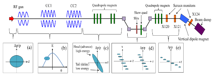
Figure 1: Layout of the FAST photoinjector.

3 Micro-bunched beam production

In this section, we present the theory and the method of creating and observing a micro-bunched beam using an energy chirped bunch, a slit-mask and a skew quadrupole in the magnetic chicane.

3.1 Energy-chirped beam

An energy chip represents a correlation between longitudinal position $z$ and energy deviation $\delta$, and is defined by $h=\partial\delta/\partial z|_{z=0}$. This correlation can be produced by accelerating the beam with an off-crest rf phase in a cavity (see (a), (b), and (c) in Fig. 1).

We define $E_{0,ref},E_{1,ref},E_{2,ref}$ to be the nominal beam energies at the entry of CC1, exit of CC1, and the exit of CC2 respectively. The reference particle at the longitudinal center ($z=0$) of the bunch has the nominal energy while a particle at an arbitrary position $z$ has energies $E_{1}(z),E_{2}(z)$ after CC1 and CC2 respectively.

$$E_{1}(z) = E_{0,ref}(1+\delta_{0})+eV_{1,rf}\cos(\phi_{1,rf}-k_{rf}z),$$ (1)

$$E_{2}(z) = E_{1}(z)+eV_{2,rf}\cos(\phi_{2,rf}-k_{rf}z),$$ (2)

where $\delta_{0}$ is the initial energy deviation (due to the uncorrelated energy spread from the rf gun), $(V_{1,rf},V_{2,rf})$ are the the voltages and $(\phi_{1,rf},\phi_{2,rf})$ are the rf phases in CC1, CC2 respectively. $k_{rf}$ is the rf wave number, the same for both cavities. The relative energy deviations from the nominal energy after CC1 and CC2 are given by $\delta_{1}(z)=(E_{1}(z)-E_{1,ref})/E_{1,ref}$ and $\delta_{2}(z)=(E_{2}(z)-E_{2,ref})/E_{2,ref}$ respectively. Therefore, the energy chirp $h_{1}$ after CC1 and the total chirp $h_{T}$ after CC2 can be written as

$$h_{1} \equiv \frac{\partial\delta_{1}}{\partial z}|_{z=0}=\frac{k_{rf}v_{1}\sin\phi_{1,rf}}{1+v_{1}\cos\phi_{1,rf}},$$ (3)

$$h_{T} \equiv \frac{\partial\delta_{2}}{\partial z}|_{z=0}=\frac{k_{rf}[v_{1}\sin\phi_{1,rf}+v_{2}\sin\phi_{2,rf}]}{1+v_{1}\cos\phi_{1,rf}+v_{2}\cos\phi_{2,rf}},$$ (4)

where $v_{i}=eV_{i,rf}/E_{0,ref},i=1,2$ are dimensionless parameters. In Eqs. (3, 4). $h<0$(respectively $h>0$) means that higher energy (respectively lower energy) electrons are in the bunch head after the cavity, which leads to bunch lengthening (respectively shortening) (see (c) in Fig. 1). The energy chirp for the maximum compression of an electron beam is $h=-1/RC_{56}\simeq 5.6\,\mathrm{m^{-1}}$ at FAST, where $RC_{56}$ is the longitudinal dispersion generated by the chicane.

The energy chirp can be produced by accelerating with an off-crest phase in either one or both cavities. Since off-crest acceleration lowers the beam energy, the two accelerating voltages are changed to keep the final energy fixed at 35 MeV which is the value for $\phi_{1,rf}=\phi_{2,rf}=\pm 35^{\circ}$ at the peak voltage gradients shown in Table 1. The constant beam energy simplifies operation by requiring no tuning of the dipole strengths in the chicane for each choice of rf phases. The energy chirps calculated with Eqs. (3, 4) are summarized in Table 2 in Section 5.

3.2 Micro-bunched beam

The energy-chirped beam from the two cavities is sent to the chicane where the horizontal dispersion has negative values. Electrons in the chicane are separated horizontally with higher energy (lower energy) electrons passing through the inside (outside) of the ideal orbit. The slit-mask in the middle of the chicane splits the beam horizontally into sections (see (d) in Fig. 1). Beam transmission through the slit-mask is expected to be around 5% from the ratio of the slit width $W$ to the slit spacing $D$. The particles passing through a slit opening are fully transmitted since the beam divergence at the slit-mask (= 0.7 mrad) is much smaller than the opening angle $W/t=0.1$ rad where $t$ is the thickness of the slit, while the particles passing through the tungsten are scattered at large angles and lost downstream of the mask. This transmission ratio has been confirmed with Geant4 simulations [24].

In the bunch lengthening mode of operation, higher energy electrons after the chicane are at the bunch head while the lower energy electrons are at the bunch tail. The horizontally separated bunch after the slit-mask is transformed into a longitudinally separated beam (or into micro-bunches) after the chicane (see (e) in Fig. 1). The lengthening increases the longitudinal separation between the micro-bunches.

The longitudinal width and spacing of the micro-bunches can be found using the transfer matrix. The 6$\times$6 transfer matrix of the dogleg (from the entrance of the chicane to the slit-mask in the middle of the chicane) composed of rectangular bend magnets transforms the six dimensional phase space variables $(x,x^{\prime},y,y^{\prime},z,\delta)$ as

$$\left(\begin{array}[]{c}x\\ x^{\prime}\\ y\\ y^{\prime}\\ z\\ \delta\end{array}\right)_{s}=\left(\begin{array}[]{cccccc}1&R_{12}&0&0&0&R_{16}\\ 0&1&0&0&0&0\\ 0&0&R_{33}&R_{34}&0&0\\ 0&0&R_{43}&R_{44}&0&0\\ 0&R_{52}&0&0&1&R_{56}\\ 0&0&0&0&0&1\\ \end{array}\right)\left(\begin{array}[]{c}x\\ x^{\prime}\\ y\\ y^{\prime}\\ z\\ \delta\end{array}\right)_{1}.$$ (23)

The matrix elements are given by

$$R_{12} = d_{1}+\frac{1}{2}d_{2}+2\rho\sin\theta,\;\;\;R_{16}=-2(d_{1}+\rho\sin\theta)\tan(\frac{\theta}{2})$$

$$R_{33} = \cos 2\theta-\frac{(d_{1}+d_{2})}{2\rho}\sin 2\theta+\frac{d_{1}d_{2}}{2\rho^{2}}\sin^{2}\theta$$

$$R_{34} = d_{1}\cos^{2}\theta+\rho\sin 2\theta+\frac{d_{2}}{2}\cos 2\theta-\frac{d_{1}d_{2}}{4\rho}\sin 2\theta$$

$$R_{43} = \frac{d_{1}}{\rho^{2}}\sin^{2}\theta-\frac{1}{\rho}\sin 2\theta,\;\;\;R_{44}=\cos 2\theta-\frac{d_{1}}{2\rho}\sin 2\theta,\;\;\;R_{52}=R_{16},$$

$$R_{56} = 4(d_{1}+2\rho\sin\theta)\tan^{2}\frac{\theta}{2}-2\rho(\beta_{k}^{2}\theta-\sin\theta)+\frac{1}{\gamma^{2}}(d_{1}+\frac{1}{2}d_{2}).$$ (24)

In the above, we assumed a symmetric chicane with the same magnitude of the bend angle $\theta$ and bend radius $\rho$ in each dipole and where the separation $d_{1}$ between the first and second dipoles is the same as that between the third and fourth dipoles and $d_{2}$ is the separation between the second and third dipoles. $\gamma$ is the beam’s relativistic Lorentz factor in the chicane. This is large enough that the third term in $R_{56}$ is negligible. We find that second order chromatic terms such as $T_{166},T_{566}$ are larger than but are of the same order of magnitude as the first order terms, so their influence on the dynamics is likely to be negligible for the usual beam energy spreads.

The horizontal position of a particle at the slit-mask is given by $x_{s}=x_{c}+R_{16}\delta_{1}$, where $x_{c}=x_{1}+R_{12}x^{\prime}_{1}$, and where $(x_{1},x^{\prime}_{1})$ are the horizontal coordinates of the particle at the chicane’s entrance. The energy deviation (constant through the chicane) is $\delta_{1}(=\delta_{s})=\delta_{0}+hz_{1}$, where $\delta_{0}$ is the deviation due to the uncorrelated energy spread, $h$ is the energy chirp, and $z_{1}$ is the longitudinal coordinate of the particle at the chicane entrance. In terms of the transverse positions and $\delta_{0}$, this can be written as

$$z_{1}=\frac{(x_{s}-x_{c})}{hR_{16}}-\frac{\delta_{0}}{h}.$$ (25)

The transfer matrix $RC$ for the complete chicane can be similarly written down. For our purposes, the non-zero elements of interest are in the $(x,x^{\prime},z,\delta)$ planes

$$RC_{11}=1,\;\;\;RC_{12}=2R_{12},\;\;\;RC_{22}=1,$$

$$RC_{55}=1,\;\;\;RC_{56}=2R_{56},\;\;\;RC_{66}=1\;,$$ (26)

where $R_{12},R_{56}$ are given by the expressions in Eq. (24). The other non-zero elements $(RC_{33},RC_{34},RC_{43},RC_{44})$ are not needed here and are omitted.

The longitudinal coordinate $z_{2}$ after the chicane is

$$z_{2} = z_{1}+RC_{56}\delta_{1}=\frac{(1+hRC_{56})}{hR_{16}}(x_{s}-x_{c})-\frac{\delta_{0}}{h}$$ (27)

$$= \frac{(1+hRC_{56})}{hR_{16}}(x_{s}-x_{1})-\frac{R_{12}(1+hRC_{56})}{hR_{16}}x_{1}^{\prime}-\frac{\delta_{0}}{h}.$$

In Eq.(27), only the variables $x_{1},x_{1}^{\prime}$ have a non-zero covariance, the other variables are uncorrelated. Since the full slit width $W$ is smaller than the the rms beam size, we can assume that the beam distribution in the slits is uniform. We have for the variances and the non-zero covariance,

$$\langle x_{s}^{2}\rangle = \frac{W^{2}}{12},\;\;\;\;\;\langle\delta_{0}^{2}\rangle=\sigma^{2}_{\delta,U}$$ (28)

$$\langle x_{1}^{2}\rangle = \beta_{1}\varepsilon,\;\;\;\langle(x_{1}^{\prime})^{2}\rangle=\frac{1+\alpha_{1}^{2}}{\beta_{1}}\varepsilon,\;\;\;\langle x_{1}x_{1}^{\prime}\rangle=-\alpha_{1}\varepsilon$$ (29)

where $\beta_{1},\alpha_{1}$ are the horizontal beta and alpha functions at the chicane entrance, $\varepsilon$ is the un-normalized horizontal emittance, and $\sigma_{\delta,U}$ is the uncorrelated rms relative energy spread in the chicane. We obtain the rms length of a micro-bunch $\sigma_{z_{2},MB}$ from

$$\sigma_{z,MB}^{2} = \left[\frac{(1+hRC_{56})}{h\eta}\right]^{2}\times\left\{\frac{W^{2}}{12}+\varepsilon\left[\beta_{1}-2R_{12}\alpha_{1}+R_{12}^{2}\frac{1+\alpha_{1}^{2}}{\beta_{1}}\right]\right\}+\frac{\sigma^{2}_{\delta,U}}{h^{2}}$$ (30)

$$= \left[\frac{(1+hRC_{56})}{h\eta}\right]^{2}\times\left\{\frac{W^{2}}{12}+\varepsilon\beta_{S}\right\}+\frac{\sigma^{2}_{\delta,U}}{h^{2}},$$

where $\eta=R_{16}=-2(d_{1}+\rho\sin\theta)\tan(\theta/2)$ is the dispersion at the slits and $\beta_{S}=\beta_{1}-2R_{12}\alpha_{1}+R_{12}^{2}(1+\alpha_{1}^{2})/\beta_{1}$ is the beta function at the slits. In most cases, the contribution of the betatron size dominates, so that we have approximately

$$\sigma_{z,MB}\approx\frac{|(1+hRC_{56})|}{|\eta h|}\sqrt{\beta_{S}\varepsilon}\;.$$ (31)

Eq. (30) shows that $\varepsilon\beta_{S}$ and $\sigma_{\delta,U}$ should be small to minimize the length of each micro-bunch and therefore create larger longitudinal separations between the micro-bunches.

Denoting the horizontal position at the $i$th slit by $x_{s}^{i}$, we have on average $\langle x_{s}^{i}-x_{s}^{i-1}\rangle=D$ where $D$ is the slits spacing, while $\langle x_{c}^{I}-x_{c}^{I-1}\rangle=0$. Hence the average longitudinal separation $\langle\Delta z\rangle$ after the chicane between particles which pass through neighboring slits is

$$|\langle\Delta z\rangle|=|\langle(z^{i}_{2}-z^{i-1}_{2})\rangle|=\frac{D}{|h\eta|}(|1+hRC_{56}|).$$ (32)

Here we have dropped the negligible differences in energy between particles at neighboring slits. The micro-bunched beam’s widths and spacings computed for each energy chip are summarized in Table 2 in Section 5.

3.3 Frequency dependence on energy chirp

THz radiation can be generated by allowing the micro-bunched beam to traverse an Al foil. The fundamental frequency $f_{0}$ is determined by the separation between the micro-bunches for a comb structure beam and is given by

$$f_{0}=\frac{c}{|\langle\Delta z\rangle|}=\frac{c|h\eta|}{D|1+hRC_{56}|}.$$ (33)

This equation is valid as long as the separation satisfies $|\langle\Delta z\rangle|\gg RC_{56}\sigma_{\delta,U}$ which is generally true, except in the vicinity of maximum compression where $\langle\Delta z\rangle\rightarrow 0$. Figure 2 shows the fundamental frequency as a function of the energy chirp. The fundamental frequency can be changed by varying the energy chirp. From Fig. 2, the fundamental frequencies are about 0.3 THz, 0.33 THz, and 0.38 THz at negative chirps $h$=-7, -9, and -16 $\mathrm{m}^{-1}$, respectively, and 1.82 THz, 1.27 THz, and 0.77 THz at positive chirps $h$=7, 9, and 16 $\mathrm{m}^{-1}$, respectively. The fundamental frequency is zero when there is no chirp (at $h=0\,\mathrm{m}^{-1}$ ) and goes to large values close to maximum compression as $h\rightarrow-1/(RC_{56})\sim 5.6\,\mathrm{m}^{-1}$. While positive $h$ values lead to larger fundamental frequencies, they also compress the entire bunch structure and lead to overlap between micro-bunches, and the frequency spectra are broadband rather than narrow-band. Figure 2 also shows that the fundamental frequency changes slowly beyond $|h|\approx 20$ m^-1, so there is no advantage in going beyond these chirp values. The fundamental frequencies computed for each energy chirp are summarized in Table 2 in Section 5.

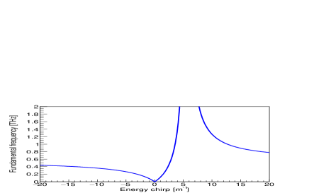
Figure 2: Fundamental frequency depending on energy chirps. The fundamental frequency becomes large near the maximum compression at $h=5.6$ m^-1.

3.4 Observing micro-bunching in the transverse plane

A skew quadrupole magnet installed in the chicane can be used to confirm that a micro-bunched beam is produced prior to detecting the radiation. When the skew quadrupole is turned on in the chicane where the horizontal dispersion is non-zero, vertical dispersion is generated downstream of the skew quadrupole via beam coupling. Due to the vertical dispersion after the chicane, the information on the beam separation in the horizontal plane (energy-plane) at the skew quadrupole is transferred to the vertical plane [25]. Using a Yttrium Aluminum Garnet (YAG) scintillating screen downstream of the chicane, we can observe the electron beam separation in the vertical plane. The vertical spacing can be found through the transfer matrix from the skew quadrupole in the chicane to the monitor downstream of the chicane. The phase space vectors at the monitor and slit locations are related via

$$\left(\begin{array}[]{c}x\\ x^{\prime}\\ y\\ y^{\prime}\\ z\\ \delta\end{array}\right)_{M} = RM\cdot\left(\begin{array}[]{cccccc}1&0&0&0&0&0\\ 0&1&-k_{S}&0&0&0\\ 0&0&1&0&0&0\\ -k_{S}&0&0&1&0&0\\ 0&0&0&0&1&0\\ 0&0&0&0&0&1\\ \end{array}\right)\left(\begin{array}[]{c}x\\ x^{\prime}\\ y\\ y^{\prime}\\ z\\ \delta\end{array}\right)_{s}.$$ (52)

The non-zero components of the matrix $RM$ are

$$RM_{11} = 1,\;\;\;RM_{12}=R_{12}+d_{M},\;\;\;RM_{16}=-R_{16},\;\;\;RM_{22}=1,$$

$$RM_{33} = \cos 2\theta-\frac{d_{1}}{2\rho}\sin 2\theta+\frac{d_{M}}{\rho^{2}}(d_{1}\sin^{2}\theta-\rho\sin 2\theta)$$

$$RM_{34} = R_{34}+d_{M}R_{33}$$

$$RM_{43} = R_{43},\;\;\;RM_{44}=\cos 2\theta+\frac{1}{2\rho^{2}}[d_{1}d_{2}\sin^{2}\theta-(d_{1}+d_{2})\rho\sin 2\theta]$$

$$RM_{52} = -R_{52},\;\;\;RM_{55}=1,\;\;\;RM_{56}=R_{56}+\frac{d_{M}}{\gamma^{2}},\;\;\;RM_{66}=1,$$ (53)

where $k_{S}$ is the inverse focal length of the skew quadrupole, $d_{M}$ is the distance from the end of the chicane to the monitor, and the matrix elements $R_{ij}$ are those in Eq. (24). The vertical position $y_{M}$ at the monitor after the chicane is,

$$y_{M} = -k_{S}RM_{34}x_{s}+RM_{33}y_{s}+RM_{34}y^{\prime}_{s}=y_{2,k_{S}=0}-k_{S}RM_{34}x_{s}.$$ (54)

$$y_{2,k_{S}=0} = RM_{33}y_{s}+RM_{34}y^{\prime}_{s}.$$

Taking the effect of the slit-mask into account, the average vertical spacing is

$$\langle\Delta y\rangle = \langle(y^{i}_{M_{k_{S}=0}}-y^{i-1}_{M_{k_{S}=0}})-k_{S}RM_{34}(x^{i}_{s}-x^{i-1}_{s})\rangle$$

$$\Rightarrow|\langle\Delta y\rangle| = |k_{S}|D\;RM_{34}\;.$$ (55)

where $D$ is the horizontal spacing of the slits and we used $\langle(y^{i}_{M_{,}k_{S}=0}-y^{i-1}_{M_{,}k_{S}=0})\rangle=0$. The vertical average spacing is proportional to the strength of the skew quadrupole, increases with the distance $d_{M}$ to the monitor but is independent of the chirp. The electron beam should be focused vertically at the monitor to observe clearly separated slit images because the separation, determined by the second term in Eq. (54), should be larger than the first term of this equation which is determined by the betatron beam size.

The slope of the vertical separation with skew quadrupole strength can be used to infer the longitudinal separation that would be produced in the absence of this quadrupole via

$$|\langle\Delta z\rangle|=\left[\frac{|1+hRC_{56}|}{|h\eta|}\right]\left(\frac{|\langle\Delta y\rangle|}{|k_{S}|RM_{34}}\right),$$ (56)

where the terms in square brackets depend on the energy chirp and the chicane while those in parentheses depend on the observations at the transverse screen monitor.

4 Beam optics for the micro-bunched beam

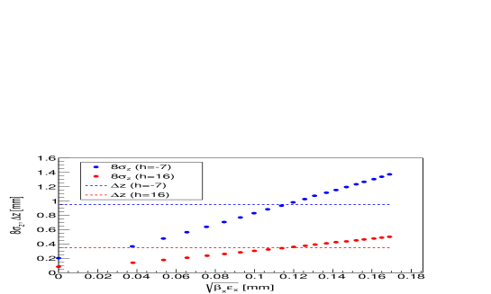
Figure 3: Spacing ($8\sigma_{z}$) and width ($\Delta z$) of micro-bunched beams as a function of $\sqrt{\beta_{x}\varepsilon_{x}}$ at the slit-mask for different energy chirps. Dots and lines represent width and spacing of micro-bunched beams, respectively.

In this section, we show the beam optics to produce a micro-bunched beam. The beam optics and particle tracking from the entrance of CC1 to the beam dump were simulated using elegant [26]. As initial parameters before CC1, we used the beam parameters shown in Table 1 while the initial Twiss functions were $\beta_{x}=\beta_{y}=4.89\,\mathrm{m}$, and $\alpha_{x}=\alpha_{y}=0$. These beta functions are chosen so that the electron beam sizes at the entrance of CC1 are 1 mm in each plane. The accelerating voltages in CC1 and CC2 are tuned so that the electron beam energy stays constant at 35 MeV, as mentioned in Section 3.

Clear separations of the micro-bunches after the chicane require that the total width of a micro-bunch to be smaller than the micro-bunch spacing $\langle\Delta z\rangle$. We set $8\sigma_{z,MB}\sim\langle\Delta z\rangle$ by controlling $\beta_{x}$ at the slit-mask. Figure 3 shows the relation between total width ($8\sigma_{z}$) of micro-bunched beams and betatron beam size $\sqrt{\varepsilon_{x}\beta_{x,S}}$ for different energy chirps. Dots and lines represent widths and spacings of micro-bunched beams, respectively. From Fig. 3, we chose $\beta_{x,S}=0.5\,\mathrm{m}$ at the slits so that the betatron beam size $\sqrt{\varepsilon_{x}\beta_{x,S}}=0.12$ mm at the intersection of $8\sigma_{z}$ and $\langle\Delta z\rangle$ for energy chirps except for those close to $h=+5.6\,\mathrm{m}^{-1}$ at the maximum compression where $\langle\Delta z\rangle=0$. When the energy chirps are $h=+7,+9\,\mathrm{m}^{-1}$, $\langle\Delta z\rangle$ is still quite small. Therefore, correspondingly small values of $\varepsilon_{x}\beta_{x}$ and uncorrelated energy spread $\sigma_{\delta,U}$ are required to obtain a clearly separated longitudinal distribution after the chicane.

Figure 4 shows the beam optics from CC1 to the beam dump at $h=-7\,\mathrm{m^{-1}}$ with a chirp only in CC1. The beam optics for different energy chirps shows similar behavior. The horizontal beta function for all cases is focused to about 0.5 m at the slit-mask. We also focused the vertical beam size at the screen monitor X120 downstream of the chicane to be as small as possible for clear separations of the vertical slit images when the skew quadrupole is turned on.

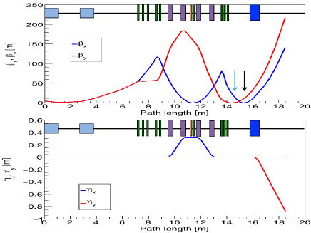
Figure 4: Beta and dispersion functions at $h=-7\,\mathrm{m^{-1}}$ for CC1 chirp. Blue and red lines show horizontal and vertical planes respectively. Light blue, green, magenta boxes show the accelerating structures, (normal and skew) quadrupole magnets, and dipole magnet of the chicane, respectively. The navy blue box at $\sim 16$m represents the vertical bend magnet which sends the beam to the dump.

5 Simulations of micro-bunched beams

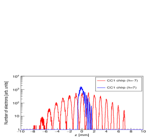
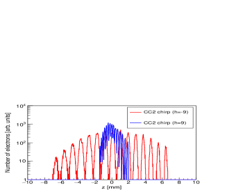
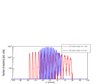
Figure 5: Longitudinal distributions at CC1 chip ($h=\pm 7\,\mathrm{m^{-1}}$), CC2 chirp ($h=\pm 9\,\mathrm{m^{-1}}$), and CC1&CC2 chips ($h=\pm 16\,\mathrm{m^{-1}}$). Red lines are the bunch lengthening mode, and blue lines are the over compressed mode.

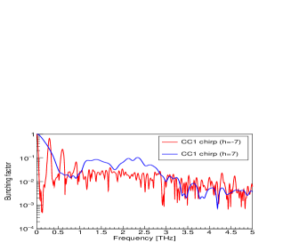
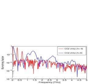
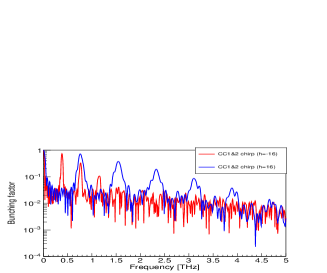
Figure 6: Bunching factors for CC1 chip ($h=\pm 7\,\mathrm{m^{-1}}$), CC2 chirp ($h=\pm 9\,\mathrm{m^{-1}}$), and CC1&CC2 chips ($h=\pm 16\,\mathrm{m^{-1}}$). Red lines are the lengthening mode, and blue lines are the over-compressed mode.

We performed particle tracking with elegant including effects of the slit-mask, magnet nonlinearities, longitudinal space charge effects, and coherent synchrotron radiation (CSR) in the chicane. Figure 5 shows the longitudinal distributions for $h=\pm 7\,\mathrm{m}^{-1}$ (CC1 chirp), $h=\pm 9\,\mathrm{m}^{-1}$ (CC2 chirp), and $h=\pm 16\,\mathrm{m}^{-1}$ (CC1&2 chirps) at X121. Table 2 shows the width, micro-bunch spacing, and fundamental frequency obtained both by particle tracking and analytical calculations with Eq. (30, 32), and (33). The longitudinal distributions at $h=$-7, -9, and $\pm 16\,\mathrm{m}^{-1}$ are separated clearly but not at $h=$7 and 9 $\mathrm{m}^{-1}$. Moreover, the spacing and width of micro-bunches at $h=$-7, -9, and $\pm 16\,\mathrm{m}^{-1}$ obtained by particle tracking agree with those computed with Eq. (32) and (30). For the two cases of $h=$7 and 9 $\mathrm{m}^{-1}$ (over-compressed modes), the overlap between micro-bunches are caused by the small separation $\langle\Delta z\rangle$. Then, the width of micro-bunches is difficult to estimate from particle tracking correctly due to the large overlap.

Figure 6 shows the bunching factor obtained from FFTs of the longitudinal distributions for different energy chirps: $h$=$\pm$7, $\pm$9, and $\pm$16 $\mathrm{m}^{-1}$. At $h=$-7, -9 ,and $\pm 16$ $\mathrm{m}^{-1}$, narrow band frequency spectra are obtained due to well separated micro-bunches (see Fig. 5). The fundamental frequencies at the first peak obtained by particle tracking including longitudinal space charge effects are consistent with the results from Eq. 33. On the other hand, at $h=$7 and 9 $\mathrm{m}^{-1}$ where the micro-bunches overlap, the two frequency spectra have broad peaks and there are differences in the fundamental frequencies between the simulations and the analytical results. However, the spectra for positive chirps just above maximum compression are not narrow-band. These results show that using both cavities to create the chirp, i.e. $h=\pm 16$ m^-1, is most useful to create high frequency narrow-band THz radiation.

Table 2: Micro-bunch widths, spacing, and fundamental frequencies for each energy chirp. $\phi_{i,rf}=0^{\circ}$ implies on-crest RF phase. Values in parentheses show the results with longitudinal space charge (LSC), and calculated analytically with Eq. 32, 30, and 33, respectively. Initial bunch charge was 200 pC.

RF phase	Energy chirp	Width	Spacing	Fundamental freq.
$\phi_{1,rf}$, $\phi_{2,rf}$ [deg.]	[$\rm{m^{-1}}$]	[mm]	[mm]	[THz]
(+35 , +35)	-16	(0.09, 0.09)	(0.78, 0.72)	(0.39, 0.42)
(0 , +35)	-9	(0.12, 0.11)	(0.92, 0.87)	(0.33, 0.35)
(+35 , 0)	-7	(0.13, 0.12)	(1.01, 0.95)	(0.30, 0.32)
(-35 , 0)	7	(0.04, 0.02)	(0.13, 0.11)	(2.33, 2.73)
(0 , -35)	9	(0.06, 0.03)	(0.22, 0.19)	(1.37, 1.54)
(-35 , -35)	16	(0.04, 0.04)	(0.39, 0.34)	(0.76, 0.87)

Longitudinal space charge effects appear to have a negligible impact when the initial bunch charge is 200 pC. For example, the changes in the fundamental frequency are about 1% and there are no discernible differences in the bunching factor shown in Fig. 6 with or without LSC. At a bunch charge of 1 nC, the higher harmonics beyond the third get broadened and not as well defined as without the LSC inclusion. These higher harmonics will likely be beyond the high frequency cutoff imposed by vacuum windows and not of practical relevance.

6 CTR and Wiggler Radiation Spectra

In this section we examine and compare the spectra from two different radiation sources: transition radiation from an Al foil and wiggler radiation. While both of these produce broad-band radiation, the bunching factor of the micro-bunched beam considered in the previous section results in narrow band radiation which is tuned by varying the chirp in the cavities CC1 and CC2. This radiation is coherent at frequencies $f\leq c/\sigma_{z}$ where $\sigma_{z}$ is the micro-bunch rms width. In this range of frequencies, the differential energy spectrum for a bunch of $N$ electrons is given in terms of the single particle spectrum by

$$\left(\frac{d^{2}U}{d\Omega d\omega}\right)_{N}=\left(\frac{d^{2}U}{d\Omega d\omega}\right)_{1}[N+N(N-1)S(\omega)],$$ (57)

where $U$ is the energy, $\Omega$ is the solid angle, $\omega$ the angular frequency and $S(\omega)$ denotes the bunching factor.

The transition radiation spectrum for a single electron moving through an infinite metallic foil is given by the well known Ginzburg-Franck expression

$$\left(\frac{d^{2}U}{d\Omega d\omega}\right)_{1}=\frac{e^{2}}{4\pi^{3}c\epsilon_{0}}\frac{\beta^{2}\sin^{2}\theta}{(1-\beta^{2}\cos^{2}\theta)^{2}},$$ (58)

where $\beta$ is the relative velocity and $\theta$ is the horizontal angle of observation. This expression is independent of the frequency. Modifications to this spectrum due to the finite size of the foil were derived in [14] for detection both in the near field and far field. At FAST, the detector will be about 1.5 m from the source placing it in the far field at 1 THz. The radius of the foil is 1.25 cm which is comparable to the effective source size $\gamma\lambda$ at 1 THz. We find that the foil size modifications to the spectrum are quite small, so we use the Ginzburg-Franck expressions in the following calculations. Integrating Eq. (58) over the solid angle, the $N$ particle ($N\gg 1$) differential energy spectrum with respect to frequency is

$$\left(\frac{dU_{CTR}}{d\omega}\right)_{N}\simeq N^{2}\frac{e^{2}}{4\pi^{3}c\epsilon_{0}}\left[\frac{1+\beta^{2}}{\beta}\ln(\frac{1+\beta}{1-\beta})-2\right]S(\omega)$$ (59)

Here $N$ is the number of particles in each micro-bunch. Using the bunching factors shown in Fig. 6, the energy density in $\mu$J/THz for two chirp settings using both CC1 and 2 are shown in Fig. 7. Here we assumed an initial bunch charge of 1 nC and 5% transmission, so that $N=50$ pC at the foil. We discuss the possibility of choosing a mask with wider slit openings and higher transmission but lower bunching factor later in this section. The left plot in Fig. 7 shows that the energy density at the first harmonic with either chirp setting is about 0.15 $\mu$J/THz. Three harmonics are visible up to $\sim 3$ THz for both settings, but the energy density falls more slowly with frequency for the compression setting ($h=+16$), as expected. The peaks in the spectrum are at (0.39, 0.75, 1.14) THz with bunch lengthening and at (0.75, 1.53, 2.14) THz with bunch compression.

Instead of CTR, it is conceivable to use a wiggler as a broad-band source of radiation which has the advantage of higher photon flux but requires more space in the beamline. Here we provide an estimate of the energy density expected from a wiggler and compare it with the energy density from CTR. Using Eq. (3.19) in [27] and integrating over the horizontal angle, we find that the single particle spectrum in a bending magnet is

$$\frac{dU_{bend}}{d\omega} = \frac{\sqrt{3}}{2}\hbar\alpha_{f}\gamma G_{1}(\omega/\omega_{c})$$ (60)

$$G_{1}(y) = y\int_{y}^{\infty}K_{5/3}(x)dx,\;\;\;\omega_{c}=\frac{3}{2}\frac{\gamma^{3}c}{\rho}$$

Here $\alpha_{f}$ is the fine structure constant, $K_{5/3}$ is a Bessel function, $\omega_{c}$ is the critical frequency, and $\rho$ is the bend radius of the magnet. A plot of the function $G_{1}$ can be seen in Fig. 3.2 in [27]. In the approximation that the radiation from a wiggler can be viewed as the radiation from a series of $N_{P}$ bending magnets (number of periods = $N_{P}/2$), the coherent differential energy spectrum from $N$ electrons ($N\gg 1$) going through a wiggler, for frequencies $\omega<2\pi c/\sigma_{z}$ can be approximated as

$$\left(\frac{dU_{\rm{Wiggler}}}{d\omega}\right)_{N}\simeq\frac{\sqrt{3}}{2}\hbar\alpha_{f}\gamma N^{2}N_{P}G_{1}(\omega/\omega_{c})S(\omega),$$ (61)

If $\lambda_{W}$ is the length of the wiggler period, then the parameter defining the wiggler strength is $K=0.934\lambda_{W}[{\rm cm}]B_{0}[{\rm T}]$ where $B_{0}$ is the bending field. Typically $K>2.5$ describes the transition from a multiple harmonics undulator radiation to the broadband wiggler radiation. For significant THz radiation, we require a low critical frequency $\omega_{c}$ and a compact wiggler requires small values of $\lambda_{W},N_{P}$. Choosing for an example calculation, $B_{0}=0.2$ T yields the critical frequency $f_{c}=40.5$ kHz at the FAST energy and with $\lambda_{W}=15$ cm, $K=2.8$ and $N_{P}=10$ results in a wiggler length of 1.5 m. The right plot in Fig. 7 shows the energy density spectrum using Eq. (61) and the bunching factor calculated above.

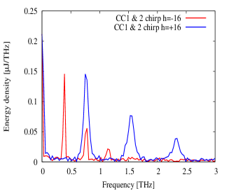
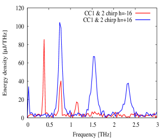
Figure 7: Energy density spectrum from two radiation sources with two chirp settings using CC1 and CC2. Charge per bunch at the radiator is 50 pC. Left: From CTR, Right: From a wiggler, $K=2.8$, length = 1.5 m.

The energy density with the wiggler at the first harmonic reaches (86, 104) $\mu$J/THz for $h=(-16,16)$ respectively, nearly three orders of magnitude higher than from CTR. However, since the angular spread of wiggler radiation is larger ($\sim K/\gamma$) than that of CTR ($\sim 1/\gamma$), the energy deposited from a wiggler can be expected to be about two orders of magnitude larger.

The slit width of the mask installed in the FAST beamline was chosen to be 50 $\mu$m spaced apart by 950 $\mu$m, primarily to increase the separation between the micro-bunches and have a large bunching factor of order one. This also results in a low transmission of 5% to the radiator. Since the coherent radiation energy scales with the square of the bunch charge and linearly with the bunching factor, it may be possible to increase the radiated energy from the above estimates by increasing the slit width for greater transmission which will also increase the overlap between the micro-bunches and reduce the bunching factor. This optimization can be done for the next iteration of the experiment with a different choice of slit mask.

We note that the bunching factor could be increased by using a longitudinal space charge amplifier (LSCA) configuration [28]. The LSCA scheme relies on the fact that the longitudinal space-charge impedance has a broad maximum approximately centered at the wavelength $\lambda_{opt}=2\pi\sigma_{\perp}/\gamma$ thereby resulting in energy modulation at wave vector amplitude around $k_{opt}=\gamma/\sigma_{\perp}$. Consequently, as the electron bunch propagates over a length $L_{d}$ while maintaining a transverse beam size $\sigma_{\perp}$, it will accumulate significant energy modulation at the wavelength $\lambda_{opt}$. This modulation can then be transferred to a longitudinal-density modulation via a dispersive section with a properly selected longitudinal dispersion $r_{56}$. This amplification process can be repeated over several stages and is characterized by a single-stage gain which, in the linear regime, takes the form $G(k)\simeq 4\pi(I_{0}/I_{A})L_{d}|Z(k)|/(\gamma Z_{0})|r_{56}|{\cal C}k\exp\left[-({\cal C}kr_{56}\sigma_{\delta})^{2}/2\right]$, where ${\cal C}\equiv(1+hr_{56})^{-1}$ is the compression factor, $I_{0}$ and $I_{A}\simeq 17$ kA are the peak and Alfven currents respectively, $Z_{0}$ is the free-space impedance. For our set of parameters, and considering the case where we wish to amplify a wavelength $\lambda_{opt}\simeq 300$ $\mu$m (1 THz) while selecting $\sigma_{\perp}$ to be at the peak of the impedance so that $|Z(k)|/Z_{0}\sim 1$, we find that the single-pass gain to be approximately $G\sim 0.5L_{d}$. Therefore, a propagation distance $L_{d}\sim 20$ m would be required to provide significant gain ($G\sim 10$). We do not consider this possibility here as it requires significant drift space with adequate optics to maintain the beam focused to the optimum spot size $\sigma_{\perp}$ and would require the addition of a small chicane. Nevertheless, we should point out combining this LSCA technique with our slit approach could also enable the selection of a wider slit size thereby increasing the overall transmitted charge and the final THz-radiation signal.

7 Simulations of micro-bunched beam observation

As discussed in Section 3, a skew quadrupole in the chicane generates vertical dispersion given by $\eta_{y}=-k_{S}RM_{34}\eta_{x}$ where $\eta_{x}$ is the horizontal dispersion at the skew quadrupole. As a result, the micro-bunches are vertically separated after the chicane. The left plot in Figure 8 shows the transverse distribution at X120 for $k_{S}$=-0.39 $\mathrm{m}^{-1}$ for $h$=-7 $\mathrm{m^{-1}}$ . The distribution is tilted to the right due to the beam coupling. The transverse distributions are similar and the vertical spacings are the same for other chirp values, as predicted by Eq. (55). The right plot in Figure 8 shows the vertical spacing of the electron beam’s dependence on the strength of the skew quadrupole from particle tracking and from Eq. (55). The vertical spacing computed with Eq. (55) is consistent with that from particle tracking. Also, the vertical spacing is proportional to the skew quadrupole strength as shown by this equation.

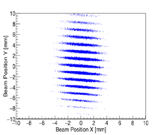
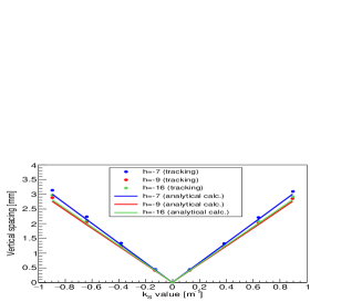
Figure 8: Left: The transverse distribution at $h$=-7 ${\mathrm{m}^{-1}}$ at $X$121 when the skew quadrupole strength $k_{S}=-0.39$ m^-1. Right: Vertical spacing as a function of $k_{S}$. Dots and lines represent the results obtained by particle tracking and analytical calculation, respectively.

8 Conclusions

In this paper, we have presented theory and simulation results related to the THz radiation experiments planned at the FAST injector. We showed that narrow-band THz radiation with a frequency of over 1 THz can be generated from a micro-bunched beam using a slit-mask placed in the chicane. Particle tracking was done using elegant and effects of magnet nonlinearities, CSR and LSC were included. We showed that the emitted frequencies can be changed by varying the energy chirps (RF phases) in the accelerating cavities. This scheme for generating narrow band tunable THz radiation is relatively simple and does not require either laser modulation of the electron bunch or variable gap undulators.

In general, lengthening the bunch with negative chirp settings results in larger separations of the micro-bunches after the chicane and spectrum peaks with narrower widths. At positive chirp settings close to the maximum compression ($h=5.6$ m^-1), there is large overlap between the micro-bunches resulting in a broad-band spectrum. However, at sufficiently large positive chirp e.g. $h=16$ m^-1, the micro-bunch widths $\sigma_{z,MB}$ and separations $\langle\Delta z\rangle$ are smaller than for $h=-16$ m^-1 but nevertheless obey $\sigma_{z,MB}\ll\langle\Delta z\rangle$, so that the spectrum peaks are well separated. Chirping in both cavities is required for either of $h=\pm 16$ m^-1. The advantage with the large negative chirp is the spectral peaks are narrower, the disadvantage is that the spectrum does not reach the higher frequencies obtained by compressing the bunch with the large positive chirp. We note that the negative chirp case is somewhat more operationally efficient since a bunch exits the rf gun with a negative chirp (i.e. higher energy particles are at the head) due to longitudinal space charge forces within the gun cavity.

A CTR foil will be used in the FAST beamline to generate the THz radiation and we calculated the expected radiation spectra for $h=\pm 16$ m^-1. Assuming a charge of 50 pC reaches the radiator, the energy density at the first harmonic for either chirp is $\sim 0.15\;\mu$J/THz. Using a relatively compact wiggler, we found that the energy density would be about three orders of magnitude higher. For both radiation sources, the power in the higher harmonics is significantly higher for bunch compression with $h=+16$ m^-1.

In the initial stage we plan to use a skew quadrupole downstream of the slit-mask in the chicane to observe micro-bunching in the vertical plane. The vertical spacing at a monitor downstream of the chicane is shown to be proportional to the skew quadrupole strength. We found that it is necessary to focus the beam vertically at the monitor to obtain clear vertical separations of the slit images but too strong focusing results in chromatic distortions of the image. However chromatic effects are quite weak when the beam is focused to spot sizes of $\sim 1$ mm (resulting in a sufficiently large high frequency cutoff $\sim$3.3 THz) at the Al target for THz production.

9 Acknowledgments

The first author would like to express his gratitude to SOKENDAI (The Graduate University of Advanced Studies) and KEK for “INTERNSHIP PROGRAM IN 2017” and to Fermilab for supporting his studies. We also thank the referee for helpful suggestions. This manuscript has been authored by Fermi Research Alliance, LLC under Contract No. DE-AC02-07CH11359 with the U.S. Department of Energy, Office of Science, Office of High Energy Physics.

References

- [1] A.-S. Muller, M. Schwarz, Accelerator-Based THz radiation Sources, in: Synchrotron Light Sources and Free-Electron Lasers, Springer, 2015, p. 31.
- [2] H. Hama, M. Yasuda, M. Kawai, F. Hinode, K. Nanbu, F. Miyahara, Intense coherent terahertz generation from accelerator based sources, Nuclear Instruments and Methods A 637 (2011) 557.
- [3] S. Antipov, S. Baryshev, R. Kostin, S. Baturin, J. Qiu, C. Jing, C. Swinson, M. Fedurin, D. Wang, Efficient extraction of high power thz radiation generated by an ultra-relativistic electron beam in a dielectric loaded waveguide, Applied Physics Letters 109 (2016) 142901.
- [4] E. Chiadroni, et al., Characterization of the thz radiation source at the Frascati linear accelerator, Review of Scientific Instruments 84 (2013) 022703.
- [5] G. L. Carr, M. C. Martin, W. R. McKinney, K. Jordan, G. R. Neil, G. P. Williams, High-power terahertz radiation from relativistic electrons, Nature 420 (2002) 153.
- [6] A. Gopal, et al., Observation of gigawatt-class THz pulses from a compact laser-driven particle accelerator, Physical Review Letters 111 (2013) 074802.
- [7] S. Antipov, M. Babzien, C. Jing, M. Fedurin, W. Gai, A. Kanareykin, K. Kusche, V. Yakimenko, A. Zholents, Subpicosecond bunch train production for a tunable mJ level THz source, Physical Review Letters 111 (2013) 134802.
- [8] Z. Wu, A. S. Fisher, J. Goodfellow, M. Fuchs, D. Daranciang, M. Hogan, H. Loos, A. Lindenberg, Intense terahertz pulses from SLAC electron beams using coherent transition radiation, Review of Scientific Instruments 84 (2013) 022701.
- [9] E. Chiadroni, et al., The SPARC linear accelerator based terahertz source, Applied Physics Letters 102 (2013) 094101.
- [10] S. Krainara, T. Kii, H. Ohgaki, S. Suphakul, H. Zen, Development of Compact THz Coherent Undulator Radiation Source at Kyoto University, in: 38th Int. Free Electron Laser Conf.(FEL’17), Santa Fe, NM, USA, August 20-25, 2017, JACOW, Geneva, Switzerland, 2018, pp. 158–161.
- [11] P. Piot, Y.-E. Sun, T. Maxwell, J. Ruan, A. Lumpkin, M. Rihaoui, R. Thurman-Keup, Observation of coherently enhanced tunable narrow-band terahertz transition radiation from a relativistic sub-picosecond electron bunch train, Applied Physics Letters 98 (2011) 261501.
- [12] M. Tonouchi, Cutting-edge terahertz technology, Nature photonics 1 (2007) 97.
- [13] N. Sei, H. Ogawa, T. Sakai, K. Hayakawa, T. Tanaka, Y. Hayakawa, K. Nogami, Millijoule terahertz coherent transition radiation at LEBRA, Japanese Journal of Applied Physics 56 (2017) 032401.
- [14] S. Casalbuoni, B. Schmidt, P. Schmüser, V. Arsov, S. Wesch, Ultrabroadband terahertz source and beamline based on coherent transition radiation, Physical Review Special Topics-Accelerators and Beams 12 (2009) 030705.
- [15] D. Xiang, G. Stupakov, Enhanced tunable narrow-band THz emission from laser-modulated electron beams, Physical Review ST - Accelerators and Beams 12 (2009) 080701.
- [16] Z. Zhang, L. Yan, W. Du, Land Huang, C. Tang, Z. Huang, Generation of high-power tunable terahertz radiation from laser interaction with a relativistic electron beam, Physical Review ST - Accelerators and Beams 20 (2017) 050701.
- [17] P. Muggli, V. Yakimenko, M. Babzien, E. Kallos, K. Kusche, Generation of trains of electron microbunches with adjustable subpicosecond spacing, Physical Review Letters 101 (2008) 054801.
- [18] P. Muggli, B. Allen, V. Yakimenko, J. Park, M. Babzien, K. Kusche, W. Kimura, Simple method for generating adjustable trains of picosecond electron bunches, Physical Review Special Topics-Accelerators and Beams 13 (2010) 052803.
- [19] J. Thangaraj, P. Piot, THz-radiation production using dispersively-selected flat electron bunches, arXiv preprint arXiv:1310.5389.
- [20] S. Antipov, et al., IOTA (Integrable Optics Test Accelerator): facility and experimental beam physics program, Journal of Instrumentation 12 (2017) T03002.
- [21] D. Crawford, et al., First beam and high-gradient cryomodule commissioning results of the Advanced Superconducting Test Accelerator at Fermilab, in: Proceedings of IPAC2015, Richmond, VA, USA, 2015, p. 1831.
- [22] B. Dwersteg, K. Flöttmann, J. Sekutowicz, C. Stolzenburg, RF gun design for the TESLA VUV Free Electron Laser, Nuclear Instruments and Methods in Physics Research Section A: Accelerators, Spectrometers, Detectors and Associated Equipment 393 (1997) 93–95.
- [23] R. Thurman-Keup, G. Kazakevich, R. Fliller, Bunch length measurement at the Fermilab A0 photoinjector using a Martin-Puplett interferometer, Tech. rep., FERMILAB-PUB-08-115-AD. (2008).
- [24] Geant4, http://geant4.cern.ch.
- [25] K. Bertsche, P. Emma, O. Shevchenko, A simple, low cost longitudinal phase space diagnostic, Tech. rep., Stanford Linear Accelerator Center (SLAC) (2009).
- [26] M. Borland, Elegant: A flexible sdds-compliant code for accelerator simulation, Tech. rep., Argonne National Lab., IL (US) (2000).
- [27] K.-J. Kim, Characteristics of synchrotron radiation, in: AIP Conference Proceedings, 184, AIP, 1989, p. 565.
- [28] E. A. Schneidmiller, M. Yurkov, Using the longitudinal space charge instability for generation of vacuum ultraviolet and x-ray radiation, Phys. Rev. ST-AB 13 (2010) 110701.