Emergent Universe by Tunneling in a Jordan-Brans-Dicke Theory

Abstract

In this work we study an alternative scheme for an Emergent Universe scenario in the context of a Jordan-Brans-Dicke theory, where the universe is initially in a truly static state supported by a scalar field located in a false vacuum. The model presents a classically stable past eternal static state which is broken when, by quantum tunneling, the scalar field decays into a state of true vacuum and the universe begins to evolve following the extended open inflationary scheme.

I Introduction

The standard cosmological model (SCM) weinberg ; peebles ; kolb and the inflationary paradigm Guth1 ; Albrecht ; Linde1 ; Linde2 are shown as a satisfactory description of our universe weinberg ; peebles ; kolb . However, despite its great success, there are still important open questions to be answered. One of these questions is whether the universe had a definite origin, characterized by an initial singularity or if, on the contrary, it did not have a beginning, that is, it extends infinitely to the past.

Theorems about spacetime singularities have been developed in the context of inflationary universes, proving that the universe necessarily has a beginning. In other words, according to these theorems, the existence of an initial singularity can not be avoided even if the inflationary period occurs, see Refs. Borde:1993xh ; Borde:1997pp ; Borde:2001nh ; Guth:1999rh ; Vilenkin:2002ev . In theses theorems it is demonstrated that null and time-like geodesics are generally incomplete in inflationary models, regardless of whether energy conditions are maintained, provided that the average expansion condition ($H>0$) is maintained throughout of these geodesics directed towards the past, where $H$ is the Hubble parameter.

The search for cosmological models without initial singularities has led to the development of the so-called Emergent Universes models (EU) Ellis:2002we ; Ellis:2003qz ; Mulryne:2005ef ; Mukherjee:2005zt ; Mukherjee:2006ds ; Banerjee:2007qi ; Nunes:2005ra ; Lidsey:2006md .

In the EU scheme it is assumed that the universe emerged from a past eternal Einstein Static (ES) state to the inflationary phase and then evolves into a hot big bang era. These models do not satisfy the geometrical assumptions of the theorems Borde:1993xh ; Borde:1997pp ; Borde:2001nh ; Guth:1999rh ; Vilenkin:2002ev and they provide specific examples of non singular inflationary universes.

Usually the EU models are developed by consider a universe dominated by a scalar field, which, during the past-eternal static regime, is rolling on the asymptotically flat part of the scalar potential (see Fig. (1)) with a constant velocity, providing the conditions for a static universe, see for example models Ellis:2002we ; Ellis:2003qz ; Mulryne:2005ef ; Nunes:2005ra ; Lidsey:2006md ; delCampo:2007mp ; delCampo:2009kp ; delCampo:2010kf ; delCampo:2011mq ; Guendelman:2011zza ; Guendelman:2011fr ; Guendelman:2013dka ; Guendelman:2014bva ; Guendelman:2015uca ; delCampo:2015yfa . Other possibility is to consider EU models in which the scale factor only asymptotically tends to a constant in the past Mukherjee:2005zt ; Mukherjee:2006ds ; Banerjee:2007sg ; Debnath:2008nu ; Paul:2008id ; Beesham:2009zw ; Debnath:2011qi ; Mukerji:2011wq ; Labrana:2013oca ; Huang:2015zma . We can note that in these schemes of Emergent Universe are not all truly static during the static regime.

At this respect a new scheme for an EU model was proposed in Ref. Labrana:2011np , where the universe is initially in a truly static state supported by a scalar field located in a false vacuum, also see Refs. Labrana:2013kqa ; Labrana:2014yta . The universe begins to evolve when, by quantum tunneling, the scalar field decays into a state of true vacuum. For simplicity, in this first approach to this new scheme of EU, the model was developed in the context of General Relativity (GR). In particular in Ref. Labrana:2011np was concluded that this new mechanism for an Emergent Universe is plausible and could be an interesting alternative to the realization of the Emergent Universe scenario.

However, as this first model was developed in the context of General Relativity, the past eternal static period, suffer from classical instabilities associated with the instability of Einstein’s static universe.

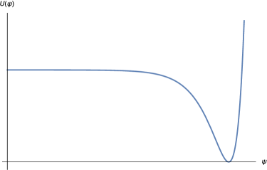
Figure 1: Schematic representation of a potential for a standard Emergent Universe scenario.

The ES solution is unstable to homogeneous perturbations, as was early discussed by Eddington in Ref. Eddington and more recently studied in Refs. Gibbons:1987jt ; Gibbons:1988bm ; Harrison:1967zz ; Barrow:2003ni . The instability of the ES solution ensures that any perturbations, no matter how small, rapidly force the universe away from the static state, thereby aborting the EU scenario.

This instability is possible to cure by going away from GR, for example, by consider a Jordan-Brans-Dicke (JBD) theory at the classical level, where it have been found that contrary to general relativity, a static universe could be classically stable, see Refs. delCampo:2007mp ; delCampo:2009kp ; Huang:2014fia .

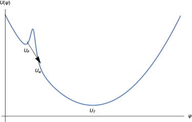
Figure 2: Scalar field potential $U(\psi)$. Here $U_{F}=U\left(\psi_{F}\right)$ and $U_{T}=U\left(\psi_{T}\right)$.

In this work, we are interested in apply the scheme of Emergent Universe by Tunneling of Ref. Labrana:2011np to EU models which present stable past eternal static regimes. In particular, we study this scheme in the context of a JBD theory, similar to the one studied in Refs. delCampo:2007mp ; delCampo:2009kp , but where the static solution is supported by a scalar field located in a false vacuum. In this case we are going to show that, contrary to what happens in Ref. Labrana:2011np , the ES solution is classically stable.

The Jordan-Brans-Dicke Jbd theory is a class of models in which the effective gravitational coupling evolves with time. The strength of this coupling is determined by a scalar field, the so-called Brans-Dicke field, which tends to the value $G^{-1}$, the inverse of the Newton’s constant. The origin of Brans-Dicke theory is found in the Mach’s principle according to which the property of inertia of material bodies arises from their interactions with the matter distributed in the universe. In modern context, Brans-Dicke theory appears naturally in supergravity models, Kaluza-Klein theories and in all known effective string actions Freund:1982pg ; Appelquist:1987nr ; Fradkin:1984pq ; Fradkin:1985ys ; Callan:1985ia ; Callan:1986jb ; Green:1987sp .

In particular in this work we are going to consider that the universe is initially in a truly static state, which is supported by a scalar field $\psi$ located in a false vacuum ($\psi=\psi_{F}$), see Fig. (2). The universe begins to evolve when, by quantum tunneling, the scalar field decays into a state of true vacuum. Then, a small bubble of a new phase of field value $\psi_{W}$ can be formed, and expands as it converts volume from high to low vacuum energy and feeds the liberated energy into the kinetic energy of the bubble wall. This process was first studied by Coleman & De Luccia in Coleman:1977py ; Coleman:1980aw in the context of General Relativity.

If the potential has a suitable form, inflation and reheating may occur inside the bubble as the field rolls from $\psi_{W}$ to the true minimum at $\psi_{T}$, in a similar way to what happens in models of Open Inflationary Universes and Extended Open Inflationary Universes, see for example linde ; re8 ; delC1 ; delC2 ; Balart:2007je , where the interior of the bubble is modeled by an open Friedmann-Robertson-Walker universe.

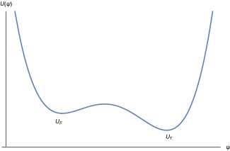
Figure 3: Potential with a false and true vacuum.

The advantage of the EU by Tunneling scheme (and of the Emergent Universe in general), over the Eternal Inflation scheme is that it correspond to a realization of a singularity-free inflationary universe. As was discussed in Refs. Borde:1993xh ; Borde:1997pp ; Borde:2001nh ; Guth:1999rh ; Vilenkin:2002ev , Eternal Inflation is usually future eternal but it is not past eternal, because in general space-time that allows for inflation to be future eternal, cannot be past null complete. On the other hand Emergent Universe are geodesically complete.

Notice that in the EU by Tunneling scheme, the metastable state which support the initial static universe could exist only a finite amount of time. Then, in this scheme of Emergent Universe, the principal point is not that the universe could have existed an infinite period of time, but that in theses models the universe is non-singular because the background where the bubble materializes is geodesically complete.

This implies that we have to consider the problem of the initial conditions for a static universe. Respect to this point, there are very interesting possibilities discussed for example in the early works on EU Ellis:2003qz and more recently in Labrana:2011np . One of these options is to explore the possibility of an Emergent Universe scenario within a string cosmology context Antoniadis . Other possibility is that the initial Einstein Static universe is created from ”nothing” Tryon ; Vilenkin-cre , see Refs. Mithani for explicit examples. It is interesting to mention that the study of the Einstein Static solution as a preferred initial state for our universe have been considered in the past, where it has been proposed that entropy considerations favor the ES state as the initial state for our universe Gibbons:1987jt ; Gibbons:1988bm .

In this paper we consider a simplified version of this scheme, with the focus on studying the process of creation and evolution of a bubble of true vacuum in the background of an ES universe in the context of a JBD theory. This is motivated because we are mainly interested in the study of new ways of leaving the static period and begin the inflationary regime for Emergent Universe models which present a classically stable static state period.

In particular, in this paper we consider a JBD theory where one of the matter content of the model is a scalar field (inflaton) with a potential similar to Fig. (3) and we study the process of tunneling of the scalar field from the false vacuum $U_{F}$ to the true vacuum $U_{T}$ and the subsequent creation and evolution of a bubble of true vacuum in the background of an stable ES universe. The simplified model studied here contains the essential elements of the scheme we want to present, so we postpone the detailed study of the inflationary period, which occurs after the tunneling, for future work.

The paper is organized as follow. In Sect. II we study a Einstein static universe supported by a scalar field located in a false vacuum and its stability in the context of a JBD theory. In Sect. III we study the tunneling process of the scalar field from the false vacuum to the true vacuum and the subsequent creation of a bubble of true vacuum in the background of the Einstein static universe for a JBD theory. In Sect. IV we study the evolution of the bubble after its materialization. In Sect. V we summarize our results.

II False Vacuum and the ES State in JBD Theories

In this paper we consider a scheme for EU scenario where the universe is initially in a classically stable static state. This state is supported by a scalar field located in a false vacuum. The universe begins to evolve when, by quantum tunneling, the scalar field decays to a state of true vacuum. For this reason we will begin by studying the possibility of obtain a static and classically stable ES solution in this theory when the scalar field is in a false vacuum.

We consider the following JBD action for a self-interacting potential and matter, given by Green:2012oqa

$$S=\int d^{4}x\sqrt{-g}\left[\frac{1}{2}\phi{\cal R}-\frac{1}{2}\frac{\omega}{\phi}\left(\nabla\phi\right)^{2}+V(\phi)+\left(\nabla\psi\right)^{2}-U(\psi)+{\cal L}_{m}\right],$$ (1)

where ${\cal R}$ is the Ricci scalar curvature, $\phi$ is the JBD field, $\omega$ is the JBD parameter, $V(\phi)$ is the potential associated to the JBD field, $\psi$ is the scalar field (inflaton), $U(\psi)$ is the scalar potential and ${\cal L}_{m}$ denotes the Lagrangian density of a barotropic perfect fluid. In this theory $1/\phi$ plays the role of the gravitational constant, which changes with time. This action also matches the low energy string action for $\omega=-1$, see Green:1987sp .

Following the EU scheme we consider a closed Friedmann-Robertson-Walker metric:

$$ds^{2}=dt^{2}-a(t)^{2}\left[\frac{dt^{2}}{1-r^{2}}+r^{2}\left(d\theta^{2}+\sin^{2}\theta d\varphi^{2}\right)\right],$$ (2)

where $a(t)$ is the scale factor and $t$ represents the cosmological time. The content of matter is modeled by a standard perfect fluid with an effective state equation given by $P_{f}=\left(\gamma-1\right)\rho_{f}$, with $\gamma$ constant, and a scalar field (inflaton) for which

$$P_{\psi}=\frac{1}{2}\dot{\psi}^{2}-U(\psi),\quad\rho_{\psi}=\frac{1}{2}\dot{\psi}^{2}+U(\psi).$$ (3)

The scalar field potential $U(\psi)$ es depicted in Fig.(2). The global minimum of $U(\psi)$ is $U_{T}$, but there is also a local minimum $U_{F}$ (the false vacuum).

We have considered that the early universe is dominated by two fluids because in our scheme of EU scenario, during the static regime, the scalar field $\psi$ remains static at the false vacuum, in contrast to standard EU models where the scalar field rolls on the asymptotically flat part of the scalar potential delCampo:2009kp . Then, in order to obtain a static universe under these conditions, we have to included a standard perfect fluid. For simplicity we will consider that there are no interactions between the standard perfect fluid and the scalar field. The Friedmann-Raychaudhuri equations become

$$H^{2}+\frac{1}{a^{2}}+H\frac{\dot{\phi}}{\phi}=\frac{\rho}{3\phi}+\frac{\omega}{6}\left(\frac{\dot{\phi}}{\phi}\right)^{2}+\frac{V}{3\phi},$$ (4)

$$2\frac{\ddot{a}}{a}+H^{2}+\frac{1}{a^{2}}+\frac{\ddot{\phi}}{\phi}+2H\frac{\dot{\phi}}{\phi}+\frac{\omega}{2}\left(\frac{\dot{\phi}}{\phi}\right)^{2}-\frac{V}{\phi}=-\frac{P}{\phi}.$$ (5)

The field equation for the JBD field is

$$\ddot{\phi}+3H\dot{\phi}=\frac{\rho-3P}{2\omega+3}+\frac{2}{2\omega+3}\left[2V-\phi V^{\prime}\right],$$ (6)

where $V^{\prime}=dV(\phi)/d\phi$, $\rho=\rho_{f}+\rho_{\psi}$, $P=P_{f}+P_{\psi}$ and dots represent derivatives with respect to cosmological time.

The conservation equations for the scalar field and perfect standard fluid are

$$\ddot{\psi}+3H\dot{\psi}=-\dfrac{\partial U(\psi)}{\partial\psi},$$ (7)

and

$$\dot{\rho_{f}}+3H\left(\rho_{f}+P_{f}\right)=0,$$ (8)

respectively.
The static universe is characterized by the conditions $a=a_{0}=\text{Const}.$, $\dot{a}_{0}=\ddot{a}_{0}=0$ and $\phi=\phi_{0}=\text{Const}.$, $\dot{\phi}_{0}=\ddot{\phi}_{0}=0$, $\psi=\psi_{F}$. From Equations (4), (5) and (6) the static solution for a universe dominated by a scalar field placed in a false vacuum and a standard perfect fluid is obtained if the following conditions are satisfied:

$$a_{0}^{2}=\frac{3}{V^{\prime}_{0}},$$ (9)

$$\rho_{f0}=-U_{F}-V_{0}+V^{\prime}_{0}\phi_{0},$$ (10)

and

$$\gamma=2\frac{\phi_{0}}{a_{0}^{2}\>\rho_{f0}},$$ (11)

where $V_{0}=V(\phi_{0})$ and $V^{\prime}_{0}=\left(dV(\phi)/d\phi\right)_{\phi=\phi_{0}}$ and $\rho_{f0}$ is the energy density of the perfect fluid present in the static universe. These equations connect the equilibrium values of the scale factor and the JBD field with the energy density and the JBD potential at the equilibrium point. We now study the stability of this solution against small homogeneous and isotropic perturbations. In order to do this, we consider small perturbations around the static solutions for the scale factor, JBD field and inflaton field.

We set

$$a(t)=a_{0}\left[1+\alpha(t)\right],$$ (12)

$$\phi(t)=\phi_{0}\left[1+\beta(t)\right],$$ (13)

$$\psi(t)=\psi_{F}[1+\lambda(t)].$$ (14)

Then, we have

$$\rho_{f}(t)=\rho_{f0}\left(\frac{a_{0}}{a(t)}\right)^{3\gamma}=\rho_{f0}\left(\frac{a_{0}}{a_{0}(1+\alpha(t))}\right)^{3\gamma}\approx\rho_{f0}\Big{(}1-3\gamma\,\alpha(t)\Big{)}=\rho_{f0}+\delta\rho_{f0}\,,$$ (15)

where $\alpha(t)\ll 1$, $\beta(t)\ll 1$ and $\lambda(t)\ll 1$ are small perturbations. On the other hand, we have that at linear order in $\lambda$

$$\delta\rho_{\psi}=2\dot{\psi}_{F}\,\delta\dot{\psi}+U^{\prime}_{F}\,\delta\psi\,,$$ (16)

$$\delta P_{\psi}=2\dot{\psi}_{F}\,\delta\dot{\psi}-U^{\prime}_{F}\,\delta\psi\,,$$ (17)

where $\delta\psi=\psi_{F}\,\lambda(t)$ and $\delta\dot{\psi}=\psi_{0}\,\dot{\lambda}(t)$. As in our case (inflaton field in a local minimum of its potential) $\dot{\psi}_{F}=0$ and $U^{\prime}_{F}=0$ then we obtain that $\delta\rho_{\psi}=\delta P_{\psi}=0$, at linear order. Then, we have that the evolution of $\lambda$ is determined only by the following equation obtained from Eq. (7) and Eq. (14)

$$\ddot{\lambda}+U^{\prime\prime}_{F}\,\lambda=0\,,$$ (18)

where $U^{\prime\prime}_{F}=\left(d^{2}U(\psi)/d\psi^{2}\right)_{\psi=\psi_{F}}$. We can note that the evolution of $\lambda$ is completely decoupled from the evolution of $\alpha$ and $\beta$ and correspond to an oscillatory behavior given that $U^{\prime\prime}_{F}>0$ in our case.

By introducing the expressions (12), (13) and (15) into equations (5) and (6), and keeping terms at the linear order in $\alpha$, $\beta$ and $\lambda$, we obtain the following set of coupled equations

$$\ddot{\alpha}-\left[\frac{1}{a_{0}^{2}}+3\frac{\left(\gamma-1\right)}{a_{0}^{2}}\right]\alpha+\frac{\ddot{\beta}}{2}-\frac{\beta}{a_{0}^{2}}=0,$$ (19)

and

$$\left(3+2\omega\right)\ddot{\beta}-\left(\frac{6}{a_{0}^{2}}-2\phi_{0}V^{\prime\prime}_{0}\right)\beta+\left(4-3\gamma\right)\frac{6}{a_{0}^{2}}\alpha=0,$$ (20)

where $V^{\prime\prime}_{0}=\left(d^{2}V(\phi)/d\phi^{2}\right)_{\phi=\phi_{0}}$.
From the system of equations (19) and (20) we can obtain the frequencies for small oscillations

$$w^{2}_{\pm}=\frac{1}{a_{0}^{2}\left(3+2\omega\right)}\left[a_{0}^{2}\phi_{0}V^{\prime\prime}_{0}-6+\omega\left(2-3\gamma\right)\right.\\ \pm\left.\sqrt{\left[-6+a_{0}^{2}\phi_{0}V^{\prime\prime}_{0}+2\omega-3\omega\gamma\right]^{2}+2\left(3+2\omega\right)\left(-6+a_{0}^{2}\phi_{0}V^{\prime\prime}_{0}\left[3\gamma-2\right]\right)}\right].$$ (21)

Note that the static solution is stable if the inequality $w_{\pm}^{2}>0$ is satisfied.
Then assuming that the parameter $\omega$ satisfies the constraint, $\left(3+2\omega\right)>0$, we find that the following inequalities must be fulfilled in order to have a stable static solution

$$\frac{2}{3}<\gamma<\frac{4}{3},\quad\gamma>\frac{4}{3}$$ (22)

$$-\frac{3}{2}<\omega<-18\frac{\left(\gamma-1\right)}{\left(2-3\gamma\right)^{2}},$$ (23)

and

$$2\left(6+\omega\right)-3\left(3+\omega\right)\gamma+\sqrt{3}\left|4-3\gamma\right|\sqrt{3+2\omega}<a_{0}^{2}\phi_{0}V^{\prime\prime}_{0}<\frac{6}{3\gamma-2}.$$ (24)

From these inequalities we can conclude that for a universe dominated by a scalar field in a false vacuum and a perfect standard fluid, it is possible to find a solution where the universe is static and stable.

In particular, we study numerical solutions to the equations (5), (6), (7) and (8), for initial conditions close to the static solution. We address the case in which the parameters take the following values that satisfy the stability conditions (22), (23) and (24)

$$\gamma=1;\quad\phi_{0}=0.5;\quad a_{0}=1;\quad U_{F}=1;\quad\psi_{F}=1,$$ (25)

where we have used units in which $8\pi G=1$. From the conditions of the static solution (9), (10), (11) and the stability condition (24) we obtain the values for $V_{0}$ , $V^{\prime}_{0}$ and $V^{\prime\prime}_{0}$.

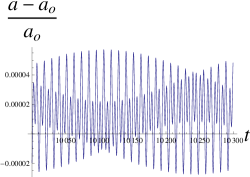
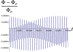
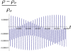
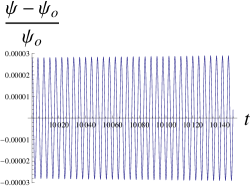
Figure 4: Behavior of the scale factor $a$, the JBD field $\phi$, the perfect fluid density $\rho$ and the inflaton field $\psi$ as a function of cosmological time.

In particular, for the numerical solution, we consider the following inflaton potential

$$U(\psi)=U_{F}+\left(\psi-\psi_{F}\right)^{2}\,,$$ (26)

where we have used that around the local equilibrium point $\psi\sim\psi_{F}$ the inflaton potential potential can be approximated to a quadratic function.

Also, we consider the following JBD potential which satisfies the static and stability conditions discussed above

$$V(\phi)=V_{0}+V^{\prime}_{0}\left(\phi-\phi_{0}\right)+\frac{V^{\prime\prime}_{0}}{2}\left(\phi-\phi_{0}\right)^{2}.$$ (27)

In Fig. (4) it is shown one numerical solution corresponding to a universe starting from an initial state not in the static solution but close to it. We can note that while the scalar field makes small oscillations around the false vacuum, the scale factor, JBD field and perfect fluid density present small oscillations around their equilibrium values. This tells us that the static solution is classically stable.

Then, in a purely classical field theory if the universe is static and supported by the scalar field located at the false vacuum $U_{F}$, the universe remains static forever. Quantum mechanics makes things different because the scalar field $\psi$ can tunnel through the barrier and by this process create a small bubble where the field value is $\psi_{T}$. Depending on the background where the bubble materializes the bubble could expand or collapse, see Refs. Labrana:2011np ; Simon:2009nb ; Fischler:2007sz .

III Bubble Nucleation

In this section we study the tunneling process of the scalar field $\psi$ from the false vacuum $U_{F}$ to the true vacuum $U_{T}$, in the potential $U(\psi)$ shown in Fig. (3) and the consequent creation of a bubble of true vacuum in the background of an Einstein static universe, in the context of a JBD Theory. In particular, we will consider the nucleation of a spherical bubble of true vacuum within the false vacuum. We will assume that the layer which separates the two phases (the wall) has a negligible thickness compared to the size of the bubble (the usual thin-wall approximation). The energy budget of the bubble consists of latent heat (the difference between the energy densities of the two phases) and surface tension.

In order to study the tunneling process in this model, we have to deal with the non-standard gravitational interaction of the JBD theory. This was done in Ref. Holman:1989gh and here we reproduce and adapt these results to the EU scheme. Regarding the study of bubble nucleation in JBD theories in other contexts see Refs. Lee:2008hz ; Kim:2010yr .

We begin with the JBD action (1) described in Sect. II and perform a weyl rescaling in order to remove the non-standard coupling of $\phi$ to $\cal R$.

$$g_{\mu\nu}=\Omega^{-2}(x)\tilde{g}_{\mu\nu},$$ (28)

$$\tilde{\phi}=\sqrt{\frac{2\omega+3}{8\pi G}}\ln\left(\phi/\phi_{G}\right),$$ (29)

where $\phi_{G}^{-1}=G$, here $G$ is the value of the Newton constant observed in the present. We choose the conformal factor $\Omega(x)$ to be $\Omega=\sqrt{8\pi G\phi}$. Then, the action in the rescaled theory can be expressed as follow

$$S[\tilde{g},\tilde{\phi},\psi]=\int d^{4}x\sqrt{-\tilde{g}}\left[\frac{1}{16\pi G}\tilde{{\cal R}}-\frac{1}{2}\tilde{g}^{\mu\nu}\tilde{\nabla}_{\mu}\tilde{\phi}\tilde{\nabla}_{\nu}\tilde{\phi}+W(\tilde{\phi})\right.\left.+\frac{b}{2}\tilde{g}^{\mu\nu}\nabla_{\mu}\psi\nabla_{\nu}\psi-b^{2}U(\psi)+b^{2}\,{\cal L}_{m}\right],$$ (30)

where we have defined

$$b\equiv\exp{\left(-4\sqrt{\frac{\pi G}{2\omega+3}}\tilde{\phi}\right)}\,,$$ (31)

$$W(\tilde{\phi})=\dfrac{V(\phi(\tilde{\phi}))}{(8\pi)^{2}G^{2}\phi^{2}}=\frac{V(\phi(\tilde{\phi}))}{(8\pi)^{2}}\exp{\left(-4\sqrt{\frac{2\pi G}{2\omega+3}}\tilde{\phi}\right)}.$$ (32)

In the rescaled theory the probability of nucleation per unit of physical volume per time is given by

$$\bar{\Gamma}(\bar{t})\equiv\dfrac{dP(\bar{t})}{d\bar{V}(\bar{t})d\bar{t}}\>,$$ (33)

where $P(\bar{t})$ is the bubble probability of nucleation and $\bar{V}(\bar{t})$ is the physical volume measured in the rescaled system at time $\bar{t}$. Therefore, the equivalent rate in the original theory is given by

$$\Gamma(t)\equiv\frac{dP(t)}{dV(t)dt}=\dfrac{dP(\bar{t})}{\left(\Omega^{3}d\bar{V}\right)\left(\Omega d\bar{t}\right)}=\Omega^{-4}(t)\bar{\Gamma}(\bar{t}),$$ (34)

where we have used that $P(t)=P\left[\bar{t}(t)\right]$, see Ref. Holman:1989gh .

In the rescaled formulation of the theory, the gravitational interaction has the standard form, and so we can expect gravitational effects similar to those of the standard theory.

Nevertheless as it is usually, in order to eliminate the problem of predicting the reaction of the geometry to an essentially a-causal quantum jump (the materialization of the bubble), we neglect during this computation the gravitational back-reaction of the bubble onto the space-time geometry. The gravitational back-reaction of the bubble will be consider in the next Section when we study the evolution of the bubble after its materialization. Thus, in this approach only the matter field $\psi$ remains as a dynamical quantity in the action (30). Then, by following Ref.Holman:1989gh we determinate the rate of nucleation of a bubble of true vacuum in the remaining dynamical theory for the field $\psi$. The nucleation rate $\bar{\Gamma}$ is given by

$$\bar{\Gamma}(t)=A\exp{\left(-S_{E}\right)}$$ (35)

where $S_{E}$ is the Euclidean action.

It is shown in Ref. Holman:1989gh that the coefficient $A$ has a net factor of $b^{2}$ with respect to a theory in which $b=1$, this entails that $\bar{\Gamma}(t)=b^{2}\Gamma_{0}$, where $\Gamma_{0}$ is the nucleation rate for a normal scalar field theory with potential $U(\psi)$. Since $b$ is a function of the time-dependent JBD field, then we have a time-dependent nucleation rate in the rescaled theory. However, this time dependence disappears if we return to the original theory. The equations (28) and (29), together with the definition of $\phi_{G}$ and $\Omega$ imply that $b=\Omega^{2}$. Using the equation (34) we find that the nucleation rate of the original theory is, see Holman:1989gh

$$\Gamma(t)=\Omega^{-4}(t)\bar{\Gamma}(\bar{t})=\left(b^{-2}\right)\left(b^{2}\Gamma_{0}\right)=\Gamma_{0}\,.$$ (36)

The computation of $\Gamma_{0}$ in the context of the EU scheme, that is, the tunneling process of the scalar field $\psi$ in a background of Einstein static universe in the context of General Relativity, was developed in Refs. Labrana:2011np ; Labrana:2013kqa ; Labrana:2014yta , where it was found that

$$\Gamma_{0}\approx\exp\left[-\frac{27\sigma^{4}\pi}{2\varepsilon^{3}}\left(1-\frac{9\,\sigma^{2}}{2\,\varepsilon^{3}\,a^{2}_{0}}\right)\right],$$ (37)

where $\varepsilon$ is the difference of energy density between the two phases (latent heat) and $\sigma$ is the energy density of the wall.

IV Classical Evolution of the Bubble on Jordan-Brans-Dicke Theories

In this section we study the evolution of true vacuum bubble after its nucleation via quantum tunnel effect. During this study we are going to consider the gravitational back-reaction of the bubble.

We follow the approach and notation used in Ref. Berezin:1987bc where it is assumed that the bubble wall separates spacetime into two parts. The bubble wall is a timelike, spherically symmetric hypersurface, the interior of the bubble is our universe, according to the extended open inflation scheme linde ; re8 ; delC1 ; delC2 ; Balart:2007je and the exterior correspond to the static universe discussed in Sec. II. In particular, we will use the scheme developed in Ref. Sakai:1992ud regarding the Darmois-Israel junction conditions Israel:1966rt ; darmois applied to a JBD Theory.

Let us start by summarize the formalism developed by Berezin, Kuzmin and Tkachev in Ref. Berezin:1987bc for the analysis of a thin wall bubble in the context of General Relativity before to study this problem in the context of a Jordan-Brans-Dicke-Theory.

We begin by defining a time-like spherically symmetric hypersurface $\Sigma$, representing the world surface of the wall dividing space-time into two regions, $V^{+}$ (outside) and $V^{-}$ (inside). Also, we define a space-like vector $N_{\mu}$, which is orthogonal to $\Sigma$ and points from $V^{-}$ to $V^{+}$. It is convenient to introduce a normal Gaussian coordinate system $\left(n,x^{i}\right)$ such that the hypersurface $n=0$ corresponds to $\Sigma$. If we assume that the wall is infinitely thin, its surface energy-momentum tensor is

$$S_{ij}\equiv\lim_{\delta\to 0}\int_{-\delta}^{\delta}\!T_{ij}\,dn.$$ (38)

Using the extrinsic curvature tensor defined by $K_{ij}\equiv N_{i;j}$ and the Einstein’s equations we can express the joint conditions on the wall as follows, see Israel:1966rt

$$\left[K_{ij}\right]^{\pm}=-\kappa^{2}\left(S_{ij}-\frac{1}{2}h_{ij}Tr\,S\right),$$ (39)

$$-S_{i|j}^{\,j}=\left[T_{i}^{\,n}\right]^{\pm},$$ (40)

$$\frac{K_{j}^{\,i\,+}+K_{j}^{\,i\,-}}{2}S_{i}^{j}=\left[T_{n}^{\,n}\right]^{\pm},$$ (41)

where $\kappa^{2}\equiv 8\pi G$, $h_{ij}$ is the 3-metric on $\Sigma$, and $|$ denotes the three-dimensional covariant derivative. We use the brackets to represent the difference between the outer and inner values of any field variable, for example: $\left[F\right]^{\pm}\equiv F^{+}-F^{-}$. By using Eq.(39) and Eq.(41) we eliminate $K_{j}^{\,i\,-}$ obtaining:

$$K_{j}^{\,i\,+}S_{i}^{j}+\frac{\kappa^{2}}{2}\left\{S_{j}^{i}S_{i}^{j}-\frac{1}{2}\left(Tr\,S\right)^{2}\right\}=\left[T_{n}^{\,n}\right]^{\pm}.$$ (42)

Since Eq.(40) and Eq.(42) do not contain $K_{j}^{\,i\,-}$, they may be useful when the geometry of interior of the bubble is unknown.

We are going to assume that the bubble wall $\Sigma$ is spherically symmetric, then the intrinsic metric on the shell $\Sigma$ is given by

$$\left.ds^{2}\right|_{\Sigma}=d\tau^{2}-R^{2}(\tau)\left(d\theta^{2}+\sin^{2}\!\theta\,d\varphi^{2}\right),$$ (43)

where $R(\tau)$ is the radius of circumference of the wall and $\tau$ the proper time of the wall. The surface energy-momentum tensor $S_{ij}$ can be written as a perfect fluid:

$$S_{ij}=\left(\sigma-\tilde{\omega}\right)u_{i}u_{j}+\tilde{\omega}h_{ij},$$ (44)

where $\sigma$, $\tilde{\omega}$ and $u^{i}=(1,0,0)$ are the surface energy density, surface pressure and a unit time-like vector tangent to $\Sigma$, respectively. Then we can rewrite Eq.(40) and Eq.(42) as follow

$$\dfrac{d\sigma}{d\tau}+2\dfrac{dR}{d\tau}\frac{\left(\sigma+\tilde{\omega}\right)}{R}=\left[T_{\tau}^{\,n}\right]^{\pm},$$ (45)

$$-\sigma K_{\tau}^{\,\tau\,+}+2\tilde{\omega}K_{\theta}^{\,\theta\,+}+\kappa^{2}\sigma\left(\frac{\sigma}{4}+\tilde{\omega}\right)=\left[T_{n}^{\,n}\right]^{\pm}.$$ (46)

As was discussed in Ref.Berezin:1987bc , Eq.(45) and Eq.(46) determine the evolution of $\sigma$ and $R$, in the context of General Relativity, as they give us information on how its radius evolves and about the energy density that accumulates on the outer side of the wall.

In our case, in order to derive the equations of motion of the bubble wall in the Jordan-Brans-Dicke theory we are going to follow a scheme similar to that discussed above, see Ref.Sakai:1992ud .

From the JBD action Eq. (1) we obtained the following field equations

$${\cal R}_{\mu\nu}-\frac{1}{2}g_{\mu\nu}{\cal R}=\frac{1}{\phi}\tilde{T}_{\mu\nu},$$ (47)

$$\Box\phi=\frac{1}{2\omega+3}\left[Tr\textit{T}-2\phi V^{\prime}(\phi)+4V(\phi)\right],$$ (48)

where

$$\tilde{T}_{\mu\nu}\equiv\frac{\omega}{\phi}\nabla_{\mu}\phi\nabla_{\nu}\phi-\frac{\omega}{2\phi}g_{\mu\nu}\left(\nabla\phi\right)^{2}+\nabla_{\mu}\nabla_{\nu}\phi-g_{\mu\nu}\Box\phi+V(\phi)g_{\mu\nu}+T_{\mu\nu},$$ (49)

and primes denote derivatives with respect to $\phi$. In this context it is useful to introduce the following surface energy-momentum tensor defined over $\Sigma$

$$\tilde{S}_{ij}\equiv\lim_{\epsilon\to 0}\int_{-\epsilon}^{\epsilon}\!\tilde{T}_{ij}\,dn=S_{ij}-\frac{1}{2}\left(\frac{1}{2\omega+3}\right)h_{ij}Tr\textit{S},$$ (50)

where the second equality is obtained from Eq.(48) and Eq. (49). With these definitions we can use the formalism described above (for General Relativity) in order to study the evolution of the bubble in the Jordan-Brans-Dicke context, we only have to replace $T_{\mu\nu}$, $S_{ij}$ and $\kappa^{2}$ by $\tilde{T_{\mu\nu}}$, $\tilde{S_{ij}}$ y $1/\phi$, respectively. The junction condition for the Jordan-Brans-Dicke field $\phi$ is obtained from Eq(48), see Ref.suffern , in particular we obtain:

$$\phi^{+}=\phi^{-},\>\>\>\>\>\>\left[\phi_{,n}\right]^{\pm}=\frac{1}{2\omega+3}Tr\textit{S}.$$ (51)

We note from this condition that in general $V^{+}$ and $V^{-}$ can not be both homogeneous.

Now we rewrite Eq. (39), Eq. (40) and Eq. (42) in the context of a Jordan-Brans-Dicke theory

$$\left[K_{ij}\right]^{\pm}=-\frac{1}{\phi}\left(\tilde{S}_{ij}-\frac{1}{2}h_{ij}Tr\tilde{S}\right),$$ (52)

$$-\left\{\frac{\tilde{S}_{i}^{j}}{\phi}\right\}_{|j}=\frac{\left[\tilde{T}_{i}^{n}\right]^{\pm}}{\phi},$$ (53)

$$K_{j}^{i\,+}\tilde{S}_{i}^{j}+\frac{1}{2\phi}\left\{\tilde{S}_{j}^{i}\tilde{S}_{i}^{j}-\frac{1}{2}\left(Tr\tilde{S}\right)^{2}\right\}=\left[\tilde{T}_{n}^{n}\right]^{\pm}.$$ (54)

By using the equations (49) and (50), we obtain

$$\left[K_{ij}\right]^{\pm}=-\frac{1}{\phi}\left(S_{ij}-\frac{1}{2}h_{ij}\left\{1-\frac{1}{2\omega+3}\right\}Tr\textit{S}\right),$$ (55)

$$-S_{i|j}^{j}=\left[T_{i}^{n}\right]^{\pm},$$ (56)

$$K_{j}^{i\,+}S_{i}^{j}+\frac{1}{2\phi}\left(S_{j}^{i}S_{i}^{j}-\frac{1}{2}\left(TrS\right)^{2}\left\{1-\frac{1}{2\omega+3}\right\}\right)=\left[T_{n}^{n}\right]^{\pm}.$$ (57)

As was mentioned, the exterior of the bubble ($V^{+}$) is described by the metric of a closed Friedmann-Robertson-Walker universe. We write this metric as follows:

$$ds^{2}=g^{+}_{\mu\nu}dx_{+}^{\,\mu}dx_{+}^{\,\nu}=dt_{+}^{2}-a^{2}(t_{+})\left\{d\chi_{+}^{2}+r^{2}(\chi_{+})\left(d\theta^{2}+\sin^{2}\!\theta\,d\varphi^{2}\right)\right\},$$ (58)

where $r(\chi_{+})=\sin(\chi_{+})$.

We can note from the conditions (51) that if one of the regions of space-time is homogeneous the other region is not. As in our case the outer region ($V^{+}$) is a homogeneous ES universe, then the region $V^{-}$ is generally inhomogeneous.

Substituting Eq. (44) into Eq. (56) and Eq. (57), we get

$$-\sigma K_{\tau}^{\,\tau\,+}+2\tilde{\omega}K_{\theta}^{\,\theta\,+}+\frac{1}{4\phi}\sigma\left(\sigma+4\tilde{\omega}\right)+\frac{1}{2\omega+3}(-\sigma+2\tilde{\omega})^{2}=\left[\tilde{T}_{n}^{\,n}\right]^{\pm},$$ (59)

$$\dfrac{d\sigma}{d\tau}+\dfrac{dR}{d\tau}\,\frac{\left(\sigma+\tilde{\omega}\right)}{R}=\left[T_{\tau}^{\,n}\right]^{\pm}.$$ (60)

The conditions of continuity for the metric on $\Sigma$ are obtained from (43) and (58) as

$$R(\tau)=a(t_{+}(\tau))r(\chi_{+}(\tau))|_{\Sigma},\>\>\>\quad d\tau^{2}=dt_{+}^{2}-a^{2}d\chi_{+}^{2}|_{\Sigma}.$$ (61)

As usual, we consider that the content of matter in the outer region $V^{+}$ and in the inner region $V^{-}$ is a perfect fluid, with the following energy-momentum tensor

$$T^{\pm}_{\mu\nu}=\left(p^{\pm}+\rho^{\pm}\right)U^{\pm}_{\mu}U^{\pm}_{\nu}+p^{\pm}g^{\pm}_{\mu\nu},$$ (62)

where $p$, $\rho$ and $U_{\mu}$ are the pressure, energy density and 4-velocity of the perfect fluid, respectively. Then, by following Ref. Sakai:1992ud , we can rewrite Eq.(59) and Eq.(60) as

$$\dfrac{d\left(\beta_{+}v_{+}\right)}{dt_{+}}=-\beta_{+}\left\{\left(1-2\frac{\tilde{\omega}}{\sigma}\right)v_{+}H-\frac{2}{R}\dfrac{dr}{d\chi_{+}}\frac{\tilde{\omega}}{\sigma}\right\}\\ +\frac{1}{4\phi}\left\{\sigma+4\tilde{\omega}+\frac{1}{2\omega+3}\frac{\left(-\sigma+2\tilde{\omega}\right)^{2}}{\sigma}\right\}-\frac{\left[\beta^{2}\left(v^{2}\rho+p\right)\right]^{\pm}}{\sigma},$$ (63)

$$\dfrac{d\sigma}{dt_{+}}=-2\dfrac{dR}{dt_{+}}\frac{\left(\sigma+\tilde{\omega}\right)}{R}+\left[\beta v\left(\rho+p\right)\right]^{\pm},$$ (64)

$$\dfrac{dR}{dt_{+}}=\dfrac{dr}{d\chi_{+}}v_{+}+HR,$$ (65)

where

$$v_{+}\equiv a\dfrac{d\chi_{+}}{dt},\quad\beta_{+}\equiv\dfrac{dt_{+}}{d\tau}\equiv\frac{1}{\sqrt{1-v_{+}^{2}}},\quad H\equiv\dfrac{da/dt_{+}}{a}.$$ (66)

So far we have summarized the calculations of Ref. Sakai:1992ud related to the evolution of a bubble in a Jordan-Brans-Dicke theory in a general background. Now we will concentrate on our particular case, where the bubble materializes and then evolves in a background corresponding to a closed and static universe, as the one described in Sec. II.

We assume that the outer region of the bubble is static, that is

$$a\left(t\right)=a_{0},\>\>\>\phi\left(t\right)=\phi_{0},$$ (67)

with $a_{0}$ and $\phi_{0}$ constants, defined in Sec.II.

In the outer region, as content of matter we consider a scalar field $\psi$ localized in a false vacuum, and a perfect fluid, see discussion in Sec. II. Then we have

$$\rho_{+}=\rho_{f0}+U_{F}.$$ (68)

$$p_{+}=\left(\gamma_{f}-1\right)\rho_{f0}-U_{F}.$$ (69)

In the inner region, the matter content is described by the scalar field in the true vacuum ($\gamma_{-}=0)$. Then, in the inner region we have

$$p_{-}=-\rho_{-}=-U_{T}.$$ (70)

Now, we develop the derivative of the left hand side of the equation (63)

$$\dfrac{d\left(\frac{v_{+}}{\sqrt{1-v_{+}^{2}}}\right)}{dt_{+}}=\frac{v_{+}^{2}\>\dfrac{dv_{+}}{dt_{+}}}{\left(1-v_{+}^{2}\right)^{3/2}}+\frac{\dfrac{dv_{+}}{dt_{+}}}{\left(1-v_{+}^{2}\right)^{1/2}}=\frac{\dfrac{dv_{+}}{dt_{+}}}{\left(1-v_{+}^{2}\right)^{3/2}}.$$ (71)

Then the equation (63) takes the form

$$\frac{\dfrac{dv_{+}}{dt_{+}}}{\left(1-v_{+}^{2}\right)^{3/2}}=\frac{1}{\sqrt{1-v_{+}^{2}}}\left\{\frac{2}{R}\left(\tilde{\gamma}-1\right)\dfrac{dr}{d\chi_{+}}\right\}+\frac{1}{4\phi}\left\{4\tilde{\gamma}\sigma-3\sigma+\frac{\sigma}{2\omega+3}\left(-3+2\tilde{\gamma}\right)^{2}\right\}\\ +\frac{\varepsilon}{\sigma}+\frac{\gamma_{+}\rho_{+}}{\left(1-v_{+}^{2}\right)\sigma},$$ (72)

where we have defined $\varepsilon=(\rho_{+}-\rho_{-})/\sigma$.

By using $r\!\left(\chi_{+}\right)=\sin\!\left(\chi_{+}\right)$ and $R=a_{0}r$, we obtain

$$\dfrac{d\>r\left(\chi_{+}\right)}{d\chi_{+}}=\cos\!\left(\chi_{+}\right)=\sqrt{1-\sin^{2}\!\left(\chi_{+}\right)}=\sqrt{1-\left(R/a_{0}\right)^{2}}.$$ (73)

If we introduce this into the Eq. (65), we have

$$\dfrac{dR}{dt_{+}}=\sqrt{1-\left(R/a_{0}\right)^{2}}\,v_{+}.$$ (74)

We are going to consider that the matter content of the bubble wall is the same as that of the outer region ($V^{+}$), then we have $\tilde{\gamma}=\gamma_{f}$.

Therefore, we write Eq. (72) as follows

$$\frac{\dfrac{dv_{+}}{dt_{+}}}{\left(1-v_{+}^{2}\right)^{3/2}}=\frac{1}{\sqrt{1-v_{+}^{2}}}\left\{\frac{2}{R}\left(\gamma_{f}-1\right)\left(\sqrt{1-\left(R/a_{0}\right)^{2}}\right)\right\}\\ +\frac{1}{4\phi}\left\{4\,\gamma_{f}\,\sigma-3\sigma+\sigma\left(\frac{1}{2\omega+3}\right)\left(-3+2\gamma_{f}\right)^{2}\right\}+\frac{\varepsilon}{\sigma}+\frac{\gamma_{f}\,\rho_{+}}{\left(1-v_{+}^{2}\right)\sigma}.$$ (75)

Finally, Eq. (64) can be written as follows

$$\dfrac{d\sigma}{dt_{+}}=-2\left(\frac{\gamma_{f}}{R}\right)\dfrac{dR}{dt_{+}}+\frac{\gamma_{f}\,\rho_{+}v_{+}}{\sqrt{1-v_{+}^{2}}}\;.$$ (76)

The evolution of the bubble wall is completely determined, in the outside coordinates, by the equations (74)-(76). We solved these equations numerically by consider different kind of matter content for the background, satisfying the stability conditions discussed in Sec. II. From these numerical solutions we found that once the bubble has materialized in the background of an ES universe in the context of a JBD theory, it grows filling the background space.

In particular in Figs. (5)-(7) we show three examples. In the first example we consider $\gamma_{f}=0.7$ and set the following values for the radius and JBD field of the background

$$a_{0}=10,\quad\phi_{0}=0.9.$$ (77)

The results for this case are shown in the Figure (5).

In the second example, we consider $\gamma_{f}=1.3$ and the following values for the radius and the JBD field

$$a_{0}=10,\quad\phi_{0}=1.3.$$ (78)

The results for this case are shown in Figure (6).

In the third example, the matter content of the background is dust ($\gamma_{f}=1$) and we consider $a_{0}=10$ and $\phi_{0}=1.3$. The results are shown in Figure (7).

In all these examples we have assumed the following initial conditions

$$\sigma_{init}=10^{-6},\quad R_{init}=10^{-3},\quad v_{init}=10^{-2},$$ (79)

and units where $8\pi G=1$.

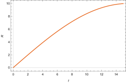
(a)

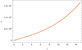
Figure 5: Evolution of the true vacuum bubble for $\gamma_{f}=0.7$. (a) Radius of the bubble as a function of time $t_{+}$. (b) Surface energy density as a function of time $t_{+}$.

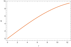
(a)

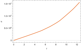
Figure 6: Evolution of the true vacuum bubble for $\gamma_{f}=1.3$. (a) Radius of the bubble as a function of time $t_{+}$. (b) Surface energy density as a function of time $t_{+}$.

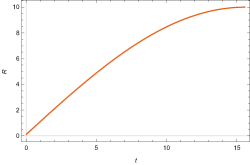
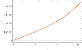
Figure 7: Evolution of the true vacuum bubble for $\gamma_{f}=1.0$. (a) Radius of the bubble as a function of time $t_{+}$. (b) Surface energy density as a function of time $t_{+}$.

From these examples we can note that the bubble of the new face, once materialized, grows to fill the background space without collapsing.

V Conclusions

In this paper we study an alternative scheme for an Emergent Universe scenario called Emergent Universe by tunneling. In this scheme the universe is initially in a truly static state supported by a scalar field which is located in a false vacuum. The universe begins to evolve when, by quantum tunneling, the scalar field decays into a state of true vacuum.

The EU by tunneling scheme was originally developed in Ref. Labrana:2013kqa , in the context of General Relativity, where it was concluded that this mechanism is feasible as an EU scheme. Nevertheless, this first model present the problem that the ES solution is classically instable. The instability of the ES solution ensures that any perturbation, no matter how small, rapidly force the universe away from the static state, thereby aborting the EU scenario.

The present work is the natural extension of the idea presented in Ref. Labrana:2013kqa , but where the problem of the classical instability of the static solution is solved by going away from General Relativity and consider a JBD theory.

In particular, in this work we focus our study on the process of tunneling of a scalar field and the consequent creation and evolution of a bubble of true vacuum in the background of a classically stable Einstein Static universe. Our principal motivation is the study of new ways of leaving the static period and begin the inflationary regime in the context of Emergent Universe models.

In the first part of the paper, Sect. II, we study an Einstein static universe supported by a scalar field located in a false vacuum and its stability in the context of a JBD theory. Contrary to General Relativity, we found that this static solution could be stable against isotropic perturbations if some general conditions are satisfied, see Eqs. (22)-(24). This modification of the stability behavior has important consequences for the emergent universe by tunneling scenario, since it ameliorates the fine-tuning that arises from the fact that the ES model is an unstable saddle in GR and it improves the preliminary model studied in Ref. Labrana:2011np . In this study, for simplicity, we have not considered inhomogeneous or anisotropic perturbations. At this respect, the stability of the ES solution under anisotropic, tensor and inhomogeneous scalar perturbations have been studied in the context of JBD theories in Refs. delCampo:2009kp ; Huang:2014fia . It was found for theses JBD models that different from General Relativity Barrow:2003ni and others modified theories of gravity as $f(R)$ Seahra:2009ft or modified Gauss-Bonnet gravity Huang:2015kca , that a static universe which is stable against homogeneous perturbations, could be also stable against anisotropic and inhomogeneous perturbations. We expect a similar behavior for our JBD model, were the static universe is supported by a scalar field located in a false vacuum. Then, we expect that in our case the inhomogeneous and anisotropic perturbations do not lead to additional instabilities. Nevertheless, we intend to return to these points in the near future by working an approach similar to that followed in Refs. Barrow:2003ni ; delCampo:2009kp ; inhomogeneous ; Huang:2014fia .

In Sect. III we study the tunneling process of the scalar field from the false vacuum to the true vacuum and the consequent creation of a bubble of true vacuum in the background of Einstein static universe for a JBD theory. In particular we determinate the nucleation rate of the true vacuum bubble using the approaches developed in Ref. Holman:1989gh and previous results obtained in Ref. Labrana:2011np .

The classical evolution of the bubble after its nucleation is studied in Sect. IV where we found that once the bubble has materialized in the background of an ES universe, it grows filling the background space. This demonstrates the viability of our EU model, since there is the possibility of having an open inflationary universe inside the bubble. During this study we consider the gravitational back-reaction of the bubble by using the formalism developed in Ref. Sakai:1992ud applied to a JBD theory. At this respect we found a system of coupled differential equations, which we solved numerically. Three specific examples of these solutions were shown in Sect. IV concerning to different background material contents.

It is worth to note that once the bubble has materialized, from conditions (51), it follows that if one of the regions of spacetime separated by the wall is homogeneous, then the other region is, in general, inhomogeneous Sakai:1992ud . Given that in our case the exterior of the bubble is a homogeneous universe, then the interior of the bubble will be, in general, inhomogeneous. However, since the degree of inhomogeneity depends on the difference in the energy density of the interior and the exterior of the bubble, it is possible in our case to decrease this inhomogeneity by adjusting the parameters of the static solution as was discussed in Ref. Sakai:1992ud . Then in our model, it is possible to study the feasibility of having an open inflationary universe inside the bubble. Nevertheless, given the similarities, we expect that the behavior inside the bubble of the EU by tunneling, will be similar to the models of single-field open and extended open inflation, as the ones studied in Refs. linde ; re8 ; delC1 ; delC2 ; Balart:2007je . We expect to return to this point in the near future.

VI Acknowledgements

P. L. is supported by Dirección de Investigación de la Universidad del Bío-Bío through Grants N⁰ 182707 4/R, and GI 172309/C. H. C. was supported by Dirección de Postgrado de la Universidad del Bío-Bío and by Research Assistant Grant of Escuela de Graduados Universidad del Bío-Bío.

References

- (1) S. Weinberg, Gravitation and Cosmology: Principle and Application of the General Relativity, Wiley, NY, 1972; Ch. W. Misner, K. S. Turner, J. A. Wheeler, Gravitation, W. H.: Freeman and Company, SF 1973.
- (2) P. J. E. Peebles, Principles of Physical Cosmology, Princeton University Press 1993; J. A. Peacock, Cosmological Physics, Cambridge University Press, 1998); S. Weinberg, Cosmology, Oxford University Press, USA, 2008.
- (3) E. Kolb and M. Turner, The Early Universe, Addison- Wesley Publishing(1989).
- (4) Guth A., The inflationary universe: A possible solution to the horizon and flatness problems, 1981 Phys. Rev. D 23 347.
- (5) Albrecht A. and Steinhardt P. J., Cosmology for grand unified theories with radiatively induced symmetry breaking, 1982 Phys. Rev. Lett. 48 1220.
- (6) Linde A. D., A new inflationary universe scenario: A possible solution of the horizon, flatness, homogeneity, isotropy and primordial monopole problems, 1982 Phys. Lett. 108B 389.
- (7) Linde A. D., Chaotic inflation, 1983 Phys. Lett. 129B 177.
- (8) Borde A. and Vilenkin A., Eternal inflation and the initial singularity, 1994 Phys. Rev. Lett. 72 3305.
- (9) Borde A. and Vilenkin A., Violation of the weak energy condition in inflating spacetimes, 1997 Phys. Rev. D 56 717.
- (10) A. H. Guth, “Eternal inflation,” Annals N. Y. Acad. Sci. 950, 66 (2001) [astro-ph/0101507].
- (11) Borde A., Guth A. H. and Vilenkin A., Inflationary space-times are incompletein past directions, 2003 Phys. Rev. Lett. 90 151301.
- (12) Vilenkin A., Quantum cosmology and eternal inflation, arXiv:gr-qc/0204061.
- (13) Ellis G. F. R. and Maartens R., The emergent universe: Inflationary cosmology with no singularity, 2004 Class. Quant. Grav. 21 223.
- (14) Ellis G. F. R., Murugan J. and Tsagas C. G., The emergent universe: An explicit construction, 2004 Class. Quant. Grav. 21 233.
- (15) Mulryne D. J., Tavakol R., Lidsey J. E. and Ellis G. F. R., An emergent universe from a loop, 2005 Phys. Rev. D 71 123512.
- (16) Mukherjee S., Paul B. C., Maharaj S. D. and Beesham A., Emergent universe in Starobinsky model, arXiv:gr-qc/0505103.
- (17) Mukherjee S., Paul B. C., Dadhich N. K., Maharaj S. D. and Beesham A. , Emergent universe with exotic matter, 2006 Class. Quant. Grav. 23 6927.
- (18) A. Banerjee, T. Bandyopadhyay and S. Chakraborty, Emergent universe in brane world scenario, Grav. Cosmol. 13, 290 (2007).
- (19) Nunes N. J., Inflation: A graceful entrance from loop quantum cosmology, 2005 Phys. Rev. D 72 103510.
- (20) Lidsey J. E. and Mulryne D. J., A graceful entrance to braneworld inflation, 2006 Phys. Rev. D 73 083508.
- (21) S. del Campo, R. Herrera and P. Labrana, “Emergent universe in a Jordan-Brans-Dicke theory,” JCAP 0711 030 (2007). [arXiv:0711.1559 [gr-qc]].
- (22) S. del Campo, R. Herrera and P. Labrana, “On the Stability of Jordan-Brans-Dicke Static Universe,” JCAP 0907 (2009) 006. [arXiv:0905.0614 [gr-qc]].
- (23) S. del Campo, E. Guendelman, R. Herrera, P. Labrana, “Emerging Universe from Scale Invariance,” JCAP 1006 (2010) 026. [arXiv:1006.5734 [astro-ph.CO]].
- (24) S. del Campo, E. I. Guendelman, A. B. Kaganovich, R. Herrera, P. Labrana, “Emergent Universe from Scale Invariant Two Measures Theory,” Phys. Lett. B699 (2011) 211-216. [arXiv:1105.0651 [astro-ph.CO]].
- (25) E. I. Guendelman, Int. J. Mod. Phys. A 26, 2951 (2011) [arXiv:1103.1427 [gr-qc]].
- (26) E. I. Guendelman, Int. J. Mod. Phys. D 20, 2767 (2011) [arXiv:1105.3312 [gr-qc]].
- (27) E. I. Guendelman and P. Labrana, Int. J. Mod. Phys. D 22 (2013) 1330018 [arXiv:1303.7267 [astro-ph.CO]].
- (28) E. Guendelman, R. Herrera, P. Labrana, E. Nissimov and S. Pacheva, Gen. Rel. Grav. 47 (2015) no.2, 10 [arXiv:1408.5344 [gr-qc]].
- (29) E. Guendelman, R. Herrera, P. Labrana, E. Nissimov and S. Pacheva, Astron. Nachr. 336 (2015) no.8/9, 810 [arXiv:1507.08878 [hep-th]].
- (30) S. del Campo, E. I. Guendelman, R. Herrera and P. Labrana, JCAP 1608 (2016) 049. [arXiv:1508.03330 [gr-qc]].
- (31) A. Banerjee, T. Bandyopadhyay, S. Chakraborty, Gen. Rel. Grav. 40, 1603-1607 (2008). [arXiv:0711.4188 [gr-qc]].
- (32) U. Debnath, Class. Quant. Grav. 25, 205019 (2008). [arXiv:0808.2379 [gr-qc]].
- (33) B. C. Paul, S. Ghose, Gen. Rel. Grav. 42, 795-812 (2010). [arXiv:0809.4131 [hep-th]].
- (34) A. Beesham, S. V. Chervon, S. D. Maharaj, Class. Quant. Grav. 26, 075017 (2009). [arXiv:0904.0773 [gr-qc]].
- (35) U. Debnath, S. Chakraborty, Int. J. Theor. Phys. 50, 2892-2898 (2011). [arXiv:1104.1673 [gr-qc]].
- (36) S. Mukerji, N. Mazumder, R. Biswas, S. Chakraborty, Int. J. Theor. Phys. 50, 2708-2719 (2011). [arXiv:1106.1743 [gr-qc]].
- (37) P. Labrana, Phys. Rev. D 91 (2015) no.8, 083534. [arXiv:1312.6877 [astro-ph.CO]].
- (38) Q. Huang, P. Wu and H. Yu, Phys. Rev. D 91, no. 10, 103502 (2015).
- (39) P. Labrana, “Emergent Universe by Tunneling,” Phys. Rev. D 86, 083524 (2012). [arXiv:1111.5360 [gr-qc]].
- (40) P. Labrana, “Tunneling and the Emergent Universe Scheme,” Astrophys. Space Sci. Proc. 38 (2014) 95.
- (41) P. Labrana, “The Emergent Universe scheme and Tunneling,” AIP Conf. Proc. 1606 (2014) 38. [arXiv:1406.0922 [astro-ph.CO]].
- (42) A. S. Eddington, Mon. Not. Roy. Astron. Soc. 90, 668 (1930).
- (43) E. R. Harrison, Rev. Mod. Phys. 39, 862 (1967).
- (44) Gibbons G. W., The entropy and stability of the universe, 1987 Nucl. Phys. B 292 784 .
- (45) Gibbons G. W., Sobolev’s inequality, Jensen’s theorem and the mass and entropy of the universe, 1988 Nucl. Phys. B 310 636.
- (46) J. D. Barrow, G. F. R. Ellis, R. Maartens and C. G. Tsagas, “On the stability of the Einstein static universe,” Class. Quant. Grav. 20, L155 (2003). [gr-qc/0302094].
- (47) H. Huang, P. Wu and H. Yu, Phys. Rev. D 89, no. 10, 103521 (2014).
- (48) Jordan P., The present state of Dirac’s cosmological hypothesis, 1959 Z.Phys. 157 112; Brans C. and Dicke R. H., Mach’s principle and a relativistic theory of gravitation, 1961 Phys. Rev. 124 925.
- (49) Freund P. G. O., Kaluza-Klein cosmologies, 1982 Nucl. Phys. B 209 146.
- (50) Appelquist T., Chodos A. and Freund P. G. O., Modern Kaluza-Klein theories ( 1987 Addison-Wesley, Redwood City).
- (51) Fradkin E. S. and Tseytlin A. A., Effective field theory from quantized strings, 1985 Phys. Lett. B 158 316.
- (52) Fradkin E. S. and Tseytlin A. A., Quantum string theory effective action, 1985 Nucl. Phys. B 261 1.
- (53) Callan C. G., Martinec E. J., Perry M. J. and Friedan D., Strings in background fields, 1985 Nucl. Phys. B 262 593.
- (54) CallanC. G., Klebanov I. R. and Perry M. J. , String theory effective actions, 1986 Nucl. Phys. B 278 78.
- (55) Green M. B., Schwarz J. H. and Witten E., Superstring theory (1987 Cambridge, Uk: Univ. Pr., Cambridge Monographs On Mathematical Physics).
- (56) S. R. Coleman, “The Fate of the False Vacuum. 1. Semiclassical Theory,” Phys. Rev. D 15, 2929 (1977) Erratum: [Phys. Rev. D 16, 1248 (1977)].
- (57) S. R. Coleman and F. De Luccia, “Gravitational Effects on and of Vacuum Decay,” Phys. Rev. D 21, 3305 (1980).
- (58) A. Linde, Phys. Rev. D 59, 023503 (1998).
- (59) A. Linde, M. Sasaki and T. Tanaka, Phys. Rev. D 59, 123522 (1999).
- (60) S. del Campo and R. Herrera, Phys. Rev. D 67, 063507 (2003).
- (61) S. del Campo, R. Herrera and J. Saavedra, Phys. Rev. D 70, 023507 (2004).
- (62) L. Balart, S. del Campo, R. Herrera, P. Labrana, J. Saavedra, “Tachyonic open inflationary universes,” Phys. Lett. B647, 313-319 (2007).
- (63) I. Antoniadis, C. Bachas, J. Ellis and D.V. Nanopolous, Phys. Lett. B 211, 4 (1988).
- (64) E.P. Tryon, Nature(London) 246, 396 (1973).
- (65) A. Vilenkin, Phys. Rev. D 32, 10 (1985).
- (66) A. T. Mithani and A. Vilenkin, JCAP 1201, 028 (2012); A. T. Mithani and A. Vilenkin, JCAP 1405, 006 (2014); A. T. Mithani and A. Vilenkin, JCAP 1507, no. 07, 010 (2015).
- (67) M. B. Green, J. H. Schwarz and E. Witten, “Superstring Theory Vol. 1 : 25th Anniversary Edition,” doi:10.1017/CBO9781139248563
- (68) D. Simon, J. Adamek, A. Rakic and J. C. Niemeyer, JCAP 0911 (2009) 008. [arXiv:0908.2757 [gr-qc]].
- (69) W. Fischler, S. Paban, M. Zanic and C. Krishnan, JHEP 0805 (2008) 041. [arXiv:0711.3417 [hep-th]].
- (70) R. Holman, E. W. Kolb, S. L. Vadas, Y. Wang and E. J. Weinberg, “False Vacuum Decay in Jordan-brans-dicke Cosmologies,” Phys. Lett. B 237, 37 (1990).
- (71) B. H. Lee and W. Lee, Class. Quant. Grav. 26, 225002 (2009) doi:10.1088/0264-9381/26/22/225002 [arXiv:0809.4907 [hep-th]].
- (72) H. Kim, B. H. Lee, W. Lee, Y. J. Lee and D. h. Yeom, Phys. Rev. D 84, 023519 (2011) doi:10.1103/PhysRevD.84.023519 [arXiv:1011.5981 [hep-th]].
- (73) V. A. Berezin, V. A. Kuzmin and I. I. Tkachev, Phys. Rev. D 36, 2919 (1987).
- (74) N. Sakai and K. i. Maeda, “Bubble dynamics in generalized Einstein theories,” Prog. Theor. Phys. 90, 1001 (1993).
- (75) W. Israel, “Singular hypersurfaces and thin shells in general relativity,” Nuovo Cim. B 44S10, 1 (1966) [Nuovo Cim. B 44, 1 (1966)] Erratum: [Nuovo Cim. B 48, 463 (1967)].
- (76) Darmois, G.“Memorial des Sciences Mathematiques” Fasc. 25, Gauthier-Villars (1927)
- (77) K. G. Suffern, J. of Phys. A15 (1982), 1599.
- (78) M. Bruni, P. K. S. Dunsby and G. F. R. Ellis, Astrophys. J. 395, 34 (1992); P. K. S. Dunsby, M. Bruni and G. F. R. Ellis, Astrophys. J. 395, 54 (1992); M. Bruni, G. F. R. Ellis and P. K. S. Dunsby, Class. Quant. Grav. 9, 921 (1992); P. K. S. Dunsby, B. A. C. C. Bassett and G. F. R. Ellis, Class. Quant. Grav. 14, 1215 (1997).
- (79) S. S. Seahra and C. G. Boehmer, Phys. Rev. D 79, 064009 (2009).
- (80) H. Huang, P. Wu and H. Yu, Phys. Rev. D 91, no. 2, 023507 (2015).