On Higgs boson plus gluon amplitudes at one loop

Abstract

We present analytic results for one-loop Higgs boson + $n$-gluon amplitudes for $n\leq 5$ in the full theory including all dependence on the (top) quark mass. In this paper we consider only the case where the gluons all have the same helicity. The amplitudes are expressed in simple formula and display similar structure. Their limiting behaviour in small Higgs momentum and large top mass is studied.

1 Introduction

It is evident that detailed study of the Higgs boson will be a primary focus of the experiments performed at the CERN LHC for at least the next decade. Many calculations of Higgs boson production by gluon fusion are carried out in the Higgs boson effective field theory, valid when the top mass is larger than all other scales in the problem. This approach has the merit that calculations performed in the effective theory are easier, since the Born-level matrix element is a tree graph, rather than a one-loop process. However, with increasing statistics the LHC will be able to probe a regime where the effective theory is no longer valid, yielding valuable information about the intermediaries circulating in the loop that couple to the Higgs boson. This is the case in Higgs boson + jet production when the transverse momentum of the Higgs boson or of the jets is large compared to the top quark mass.

Next-to-leading order (NLO) QCD corrections to Higgs boson plus 1-jet production with full top-quark mass dependence are already known Lindert:2018iug ; Jones:2018hbb . These calculations use the one-loop Higgs boson + 3 parton amplitude as the Born-level cross section, and the one-loop Higgs boson + 4 parton amplitude as a real radiation correction to the Born-level process. The two loop virtual corrections are calculated using an expansion method Lindert:2018iug or sector decomposition Jones:2018hbb . If one were to go further and calculate the NNLO QCD corrections to the Higgs boson + 1 jet process, one of the ingredients would be the Higgs boson + 5 parton amplitudes.

The Higgs + 2 jet process via gluon fusion has also been calculated at leading order in the full theory DelDuca:2001eu ; DelDuca:2001fn . This process constitutes a “background” to the Higgs + 2 jet process occurring via Vector Boson fusion, which also comes accompanied by two jets. The leading order Higgs + 3 jet process has been considered in ref. Campanario:2013mga . Phenomenological analyses of Higgs + jets including full mass effects have been performed in refs. Greiner:2015jha ; Harlander:2012hf .

Despite this progress the literature does not contain detailed analytic results for Higgs + $n$-parton amplitudes in the full theory for $n\geq 4$. Techniques for the analytic calculations based largely on unitarity have been developed over a number of years Bern:1994zx ; Bern:1994cg ; Bern:1996je ; Bern:1995db ; Britto:2004nc ; Forde:2007mi ; Badger:2008cm . The purpose of the current paper is to provide analytic results for the specific case of gluons all having the same helicity. We have undertaken this work, in order to elucidate patterns which exist for varying values of $n$. In addition, by calculating the all positive helicity processes, which are the simplest, we can assess the feasibility of obtaining simple analytic forms for all helicities.

From a numerical point of view, one loop calculations are a solved problem thanks to techniques Ossola:2006us ; Cascioli:2011va that allow numerical calculation of the coefficients of the needed loop integrals. The full numerical result is obtained by combining these numerical results for the coefficients, with analytic results for the one-loop scalar integrals. Analytic expressions for scalar one-loop integrals are completely known both for IR-finite tHooft:1978jhc and divergentEllis:2007qk cases. The downside of this semi-numerical approach is that it can lead to instabilities in corners of phase space. These instabilities can be solved by moving to higher precision calculation, at the cost of increased computer time. Analytic calculations on the other hand are less prone to these instabilities.

2 Preamble: Unitarity calculation of $H+2g$ amplitude

The aim of this paper is to calculate one-loop results for Higgs boson + gluon amplitudes. These amplitudes contain a quark of mass $m$ circulating in the loop, (dominantly the top quark) and the coupling of the Higgs boson to the quark is given by $-im/v$ where $v\approx 246$ GeV is the vacuum expectation value of the Higgs field. The mass of the Higgs boson is denoted by $M_{h}$.

We will calculate colour-ordered sub-amplitudes for the production of a Higgs boson and $n$ gluons defined as follows:

$${\cal A}_{n}(\{p_{i},h_{i},c_{i}\})\, = \,i\frac{g_{s}^{n}}{16\pi^{2}}\frac{1}{v}\sum_{\{1,2,\dots,n\}^{\prime}}\;tr\,(t^{c_{1}}t^{c_{2}}\dots t^{c_{n}})A_{n}(1_{g}^{h_{1}},2^{h_{2}}_{g},\ldots n^{h_{n}}_{g};H)\,,$$ (1)

where the sum with the prime, $\sum_{\{1,2,\dots,n\}^{\prime}}$, is over all $(n-1)!$ non-cyclic permutations of $1,2,\dots,n$ and the $t$ matrices are the SU(3) matrices in the fundamental representation normalized such that,

$$tr(t^{a}t^{b})\;=\;\delta^{ab}.$$ (2)

Because of Bose symmetry it will be sufficient to calculate one permutation, and the other colour sub-amplitudes can be obtained by exchange.

The unitarity method seeks to calculate this result by sewing together tree-level colour-ordered sub-amplitudes. For the tree graph process, $qgg\ldots g\bar{q}$, these are defined as,

$${\cal G}^{n}_{ab}(p_{a},h_{a},\{p_{i},h_{i},c_{i}\},p_{b},h_{b}) = \,ig_{s}^{n}\sum_{\sigma\in S_{n}}(t^{c_{\sigma(1)}}t^{c_{\sigma(2)}}\dots t^{c_{\sigma(n)}})_{ab}G_{n}^{\rm tree}(a_{q},\sigma(1),\ldots\sigma(n),b_{\bar{q}})\,,$$ (3)

where $S_{n}$ is the permutation group on $n$ elements, and $G_{n}^{\rm tree}$ are the tree-level partial amplitudes. In a similar way we can define the tree-level sub-amplitudes for the production of a Higgs boson and gluons from a massive fermion line,

$${\cal H}^{n}_{ab}(p_{a},h_{a},\{p_{i},h_{i},c_{i}\},p_{b},h_{b})\, = -i\frac{g_{s}^{n}}{v}\sum_{\sigma\in S_{n}}(t^{c_{\sigma(1)}}t^{c_{\sigma(2)}}\dots t^{c_{\sigma(2)}})_{ab}H_{n}^{\rm tree}(a_{q},\sigma(1),\ldots\sigma(n),H,b_{\bar{q}})\,.$$ (4)

For the case of Higgs + 2 gluons the only non-zero amplitude is when the gluons have the same helicity.

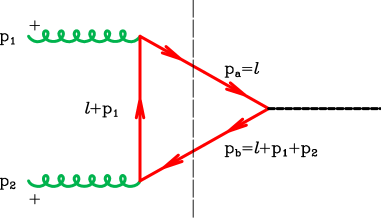
Figure 1: Unitarity approach to calculating the Higgs + 2 gluon amplitude

We sketch the calculation of this amplitude, which closely follows the approach of Bern and Morgan Bern:1995db . The relevant component tree diagrams can be extracted from Fig. 1. The left-hand side of the diagram is the colour-ordered amplitude for the $qgg\bar{q}$ process with positive helicity gluons which is given by,

$$G_{2}^{\rm tree}(a,1^{+},2^{+},b)=\frac{\left[1\,2\right]}{\left\langle 1\,2\right\rangle}\frac{\bar{u}(p_{a})\gamma_{R}(\hbox to0.0pt{$\;\!\!\not$\hss}{\mu}+m)u(p_{b})}{(s_{a1}-m^{2})},\;\;\;\gamma_{R}=(1+\gamma_{5})/2\,.$$ (5)

The components of the $d$-dimensional momenta $p_{a}$ beyond four dimensions are denoted by $\mu$ and $s_{ai}^{2}=(p_{a}+p_{i})^{2}$. With the normalization defined by Eq. (6) the right-hand side of the diagram in Fig. 1 is given by

$$H_{0}^{\rm tree}=m\bar{u}(p_{b})u(p_{a})\;.$$ (6)

Sewing Eqs. (5) and (6) together and summing over the polarizations of fermions $a$ and $b$ we get in four dimensions,

$$m^{2}\frac{\left[1\,2\right]}{\left\langle 1\,2\right\rangle}\frac{{\rm Tr}\{\gamma_{R}(\hbox to0.0pt{$\;\!\!\not$\hss}{p}_{b}+m)(\hbox to0.0pt{$\;\!\!\not$\hss}{p}_{a}+m)\}}{(s_{a1}-m^{2})}=m^{2}\frac{\left[1\,2\right]}{\left\langle 1\,2\right\rangle}\frac{(2p_{a}\cdot p_{b}+2m^{2})}{(s_{a1}-m^{2})}=m^{2}\frac{\left[1\,2\right]}{\left\langle 1\,2\right\rangle}\frac{(4m^{2}-M_{h}^{2})}{(s_{a1}-m^{2})}\,.$$ (7)

Restoring the propagators which were put on shell and exploiting the linkage between the mass terms and $\mu$, we obtain a result for the amplitude, evaluated on the two particle cut,

$$A_{2}(1^{+},2^{+};H)_{scut}=m^{2}\frac{\left[1\,2\right]}{\left\langle 1\,2\right\rangle}\frac{1}{i\pi^{2}}\int d^{d}l\frac{(4(m^{2}+\mu^{2})-M_{h}^{2})}{(l^{2}-m^{2})((l+p_{1})^{2}-m^{2})((l+p_{12})^{2}-m^{2})}\,.$$ (8)

The symbol $p_{i}$ denotes the four-momentum of the $i$th particle, and we further define, $p_{ij}=p_{i}+p_{j}$, $p_{ijk}=p_{i}+p_{j}+p_{k}$, etc. Adding in the other diagram $1\leftrightarrow 2$, and evaluating the rational term from $\mu^{2}$ we obtain,

$$A_{2}(1_{g}^{+},2_{g}^{+};H)=2m^{2}\frac{\left[1\,2\right]}{\left\langle 1\,2\right\rangle}\Big{[}(4m^{2}-M_{h}^{2})C_{0}(p_{1},p_{2};m)+2\Big{]}\;.$$ (9)

where $C_{0}$ is the scalar triangle integral, defined in Eq.(A). Note that the essential feature leading to the simple answer was the simplified form of the tree level inputs. In the following section we present the tree-level building blocks for one-loop Higgs amplitudes with greater numbers of gluons.

3 Tree level ingredients and cut techniques

3.1 Born-level results for $Q\bar{Q}$+$n$ gluon amplitudes

Multi-gluon tree amplitudes with a pair of massive fermions have been considered by a number of authors Ferrario:2006np ; Ozeren:2006ft ; Huang:2012gs using BCFW techniques and supersymmetric relations to scalar amplitudes. However since these authors make specific choices of spinors for the massive fermions they are not well suited for our purposes. All orders results for tree graphs with $n$ gluons have been given in a convenient form in ref. Ochirov:2018uyq . In our notation the $n+2$-point amplitude for a quark-antiquark pair and $n$ positive-helicity gluons is given in four dimensions by,

$$G_{n}(a\>\!\!,1^{+}\!,2^{+}\!,\dots,n^{+}\!,b)=m\frac{\bar{u}(a)\gamma_{R}u(b)\;[1|\prod_{j=1}^{n-2}\!\big{\{}\,\hbox to0.0pt{$\;\!\!\not$\hss}{p}_{a\dots j}\hbox to0.0pt{$\;\!\!\not$\hss}{p}_{j+1}+(s_{a1\dots j}-m^{2})\big{\}}|n]}{(s_{a1}\!-\!m^{2})(s_{a12}\!-\!m^{2})\dots(s_{a1\dots(n-1)}\!-\!m^{2})\,\langle 12\rangle\langle 23\rangle\dots\langle n\!-\!1|n\rangle}.\!\!$$ (10)

The important features of the all-positive helicity gluon amplitude are that the amplitude vanishes for massless quarks and that spin structure of the dependence on the massive quark momenta enters through the combination $\bar{u}(a)\gamma_{R}u(b)$ for all $n$.

For $n=2$ the product collapses to unity and we recover the four dimensional version of Eq. (5)

$$G_{2}(a,1^{+},2^{+},b)=m\frac{\bar{u}(a)\gamma_{R}u(b)}{(s_{a1}-m^{2})}\frac{\left[1\,2\right]}{\left\langle 1\,2\right\rangle}\,.$$ (11)

The results for larger numbers of gluons are similarly compact. For example, for $n=3,4$ we obtain,

$$G_{3}(a,1^{+},2^{+},3^{+},b) = m\frac{\bar{u}(a)\gamma_{R}u(b)\;[1|\left(\hbox to0.0pt{$\;\!\!\not$\hss}{p}_{a1}\hbox to0.0pt{$\;\!\!\not$\hss}{p}_{2}+(s_{a1}-m^{2})\right)|3]}{(s_{a1}-m^{2})(s_{a12}-m^{2})\;\left\langle 1\,2\right\rangle\left\langle 2\,3\right\rangle}\,.$$ (12)

$$G_{4}(a,1^{+},2^{+},3^{+},4^{+},b) = m\frac{\bar{u}(a)\gamma_{R}u(b)\;[1|\left(\hbox to0.0pt{$\;\!\!\not$\hss}{p}_{a1}\hbox to0.0pt{$\;\!\!\not$\hss}{p}_{2}+(s_{a1}-m^{2})\right)\left(\hbox to0.0pt{$\;\!\!\not$\hss}{p}_{a12}\hbox to0.0pt{$\;\!\!\not$\hss}{p}_{3}+(s_{a12}-m^{2})\right)|4]}{(s_{a1}-m^{2})(s_{a12}-m^{2})(s_{a123}-m^{2})\;\left\langle 1\,2\right\rangle\left\langle 2\,3\right\rangle\left\langle 3\,4\right\rangle}\,.$$ (13)

3.2 Interference with Higgs amplitudes

From Eq. (10) the all-positive helicity gluon amplitude has the same kinematic structure for all $n$. It is therefore useful to contract the Higgs production amplitudes with this structure,

$$M_{0}^{\dagger}=m\;\bar{u}(b)\gamma_{R}u(a)$$ (14)

We will interfere this structure with the amplitude for the production of a Higgs + 0,1 or 2 gluons. Summing over the polarizations of the massive quarks

$$\sum u(p)\bar{u}(p)=\hbox to0.0pt{$\;\!\!\not$\hss}{p}+m\,,$$ (15)

we obtain the following results for the interference with zero, one and two gluon amplitudes, $H_{0}$, $H_{1}$ and $H_{2}$,

$$M_{0}^{\dagger}\;H_{0}(a;H,b)=m^{2}\Big{(}4m^{2}-M_{h}^{2}\Big{)}\,,$$ (16)

$$M_{0}^{\dagger}\;H_{1}(a,1_{g}^{+};H,b)=m^{2}\Big{(}4m^{2}-M_{h}^{2}\Big{)}\frac{1}{\left\langle 1\,q\right\rangle}\Big{\{}\frac{[1|a|q\rangle}{[1|a|1\rangle}-\frac{[1|b|q\rangle}{[1|b|1\rangle}\Big{\}}=m^{2}\Big{(}4m^{2}-M_{h}^{2}\Big{)}\frac{[1|ab|1]}{[1|a|1\rangle\,[1|b|1\rangle}\,,$$ (17)

(where $q$ is an arbitrary light-like vector),

$$M_{0}^{\dagger}\;H_{2}(a,1_{g}^{+},2_{g}^{+};H,b)=2m^{2}\Big{(}4m^{2}-M_{h}^{2}\Big{)}\frac{1}{\left\langle 1\,2\right\rangle}\Big{\{}\frac{[2|\hbox to0.0pt{$\;\!\!\not$\hss}{b}(\hbox to0.0pt{$\;\!\!\not$\hss}{b}-\hbox to0.0pt{$\;\!\!\not$\hss}{a})|1]}{[1|a|1\rangle\,[2|b|2\rangle}$$ (18)

$$- m^{2}\left[2\,1\right]\Big{(}\frac{1}{[2|b|2\rangle\,((b-p_{12})^{2}-m^{2})}+\frac{1}{[1|a|1\rangle\,[2|b|2\rangle}-\frac{1}{[1|a|1\rangle\,((a+p_{12})^{2}-m^{2})}\Big{)}\Big{\}}\,.$$

We take all momenta to be outgoing except for $b$. We note that in four dimensions the interference of Eq. (14) with the Higgs + gluon amplitudes, $H_{n}$, is always proportional to $4m^{2}-M_{h}^{2}$.

3.3 Higgs + 4 gluon amplitude: the coefficient of the scalar pentagon

In four dimensions a scalar pentagon integral can be expressed as a sum of five boxes Melrose:1965kb ; vanNeerven:1983vr . (This reduction formula is described in appendix C). Consequently any attempt to identify the coefficient of a pentagon integral is inherently a $d$-dimensional calculation. In $d$-dimensions we must introduce an extra parameter $\mu$, that describes the magnitude of the loop momentum momentum in the $(d-4)=-2\epsilon$ space. We now use unitarity to extract the coefficient of the scalar pentagon integral for the diagram shown in Fig. 2. We express the loop momentum $l$ as,

$$l^{\nu}=\alpha\,p_{1}^{\nu}+\beta\,p_{2}^{\nu}+\frac{\gamma}{2}\,\langle 1|\gamma^{\nu}|2]+\frac{\delta}{2}\,\langle 2|\gamma^{\nu}|1]+l_{\epsilon}^{\nu}.$$ (19)

We denote the length of the component of $l$ beyond 4 dimensions, $l_{\epsilon}$, by $\mu$. Placing all five propagators on their mass shell we obtain the following five equations,

$$l^{2}-m^{2}= 0,\;\;\;\to\;\;\;\; -\gamma\delta\left\langle 1\,2\right\rangle\left[2\,1\right]-m^{2}-\mu^{2}=0\,,~{}{{\rm determines}}~{}\mu^{2}\,,$$

$$(l-p_{1})^{2}-m^{2}= 0,\;\;\;\to\;\;\;\; \beta=0\,,$$

$$(l+p_{2})^{2}-m^{2}= 0,\;\;\;\to\;\;\;\; \alpha=0\,,$$

$$(l+p_{2}+p_{3})^{2}-m^{2}= 0,\;\;\;\to\;\;\;\; \gamma\left\langle 1\,3\right\rangle\left[3\,2\right])+\delta\left\langle 2\,3\right\rangle\left[3\,1\right]+s_{23}=0\,,$$

$$(l+p_{2}+p_{3}+p_{4})^{2}-m^{2}= 0,\;\;\;\to\;\;\;\; \gamma\left\langle 1\,4\right\rangle\left[4\,2\right]+\delta\left\langle 2\,4\right\rangle\left[4\,1\right]+s_{234}-s_{23}=0\,.$$ (20)

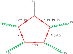
Figure 2: Feynman diagram to illustrate the calculation of coefficient the scalar pentagon integral.

However, because of the good ultraviolet properties of the pentagon integral, terms of order less than $\mu^{6}$ will play no part in the limit $\epsilon\to 0$ and can be ignored.

The pentagon coefficient of Higgs plus four gluon amplitude in Fig (2) can be calculated by putting all five propagators on-shell and sewing together the $qgggg\bar{q}$ amplitude, Eq. (13) and the projection of the Higgs production vertex, Eq. (16). After imposing the mass-shell conditions, all dependence on the loop momentum drops out and the result for the coefficient of $E_{0}(p_{1},p_{2},p_{3},p_{4};m)$ is,

$$m^{2}(4m^{2}-M_{h}^{2})\frac{[1|\hbox to0.0pt{$\;\!\!\not$\hss}{l}\,\hbox to0.0pt{$\;\!\!\not$\hss}{p_{2}}\,(\hbox to0.0pt{$\;\!\!\not$\hss}{l}+\hbox to0.0pt{$\;\!\!\not$\hss}{p_{2}})\hbox to0.0pt{$\;\!\!\not$\hss}{p_{3}}|4]}{\left\langle 1\,2\right\rangle\left\langle 2\,3\right\rangle\left\langle 3\,4\right\rangle}=-m^{4}(4m^{2}-M_{h}^{2})\frac{{\rm tr}_{+}\{{1}\,{2}\,{3}\,{4}\}}{\left\langle 1\,2\right\rangle\left\langle 2\,3\right\rangle\left\langle 3\,4\right\rangle\left\langle 4\,1\right\rangle}\,.$$ (21)

To express this formula (and subsequent formula) we have introduced a notation for the traces of gamma matrices (defined in detail in Appendix B),

$${\rm tr}_{+}\{1\,2\ldots n\}={\rm tr}\{\gamma_{R}\,\hbox to0.0pt{$\;\!\!\not$\hss}{p}_{1}\,\hbox to0.0pt{$\;\!\!\not$\hss}{p}_{2}\ldots\,\hbox to0.0pt{$\;\!\!\not$\hss}{p}_{n}\}\,.$$ (22)

The full result for the Higgs + 4 gluon amplitude is given in Eq. (27).

3.4 Higgs + 5 gluon amplitude: the coefficient of one of the scalar pentagons

We now use a similar method to identify the pentagon coefficient for the hexagon diagram shown in Fig. 3.

Figure 3: Feynman diagram to illustrate the calculation of the coefficient of the scalar integral $E_{0}(p_{1},p_{2},p_{3},p_{4};m)$

We parameterize the loop momentum as before, Eq. (19) and set the same condition on the five propagators, Eq (3.3). The condition on the propagator $l^{2}-m^{2}$ serves to fix the length of the loop momentum in the extra dimension. Solving the simultaneous equations for $\gamma$ and $\delta$ we have that,

$$\gamma = +\frac{1}{{\rm tr}_{5}(1,2,3,4)}\Big{[}\left\langle 2\,3\right\rangle\left[3\,1\right](s_{234}-s_{23})-\left\langle 2\,4\right\rangle\left[4\,1\right]s_{23}\Big{]}$$

$$\delta = -\frac{1}{{\rm tr}_{5}(1,2,3,4)}\Big{[}\left\langle 1\,3\right\rangle\left[3\,2\right](s_{234}-s_{23})-\left\langle 1\,4\right\rangle\left[4\,2\right]s_{23}\Big{]}$$ (23)

With this solution for the $\gamma,\delta$ in hand we can evaluate the sixth denominator, $d_{6}=(l+p_{2}+p_{3}+p_{4}+p_{5})^{2}-m^{2}$. The result for $d_{6}$ on the cut of the first five denominators is

$$d_{6}=-\frac{{\rm tr}_{5}(1,2,3,4,5,6)}{{\rm tr}_{5}(1,2,3,4)}\,.$$ (24)

Not surprisingly, this is inverse of the coefficient which occurs in the reduction of a scalar hexagon integral to the scalar pentagon integral formed by the first five propagators, see Eq. (D). By evaluating any possible numerators factors for the value of $l$ determined by our $\gamma,\delta$ from Eq. (3.4) we obtain the coefficient of this particular pentagon integral in our real physical amplitude. Thus determining pentagon coefficients is even easier than box coefficients, because we deal with a linear rather than a quadratic equation. The full result for the Higgs + 5 gluon amplitude is given below in Eq. (28).

4 Results for Higgs + gluon amplitudes with all positive helicity gluons

4.1 $n=2$

For the case $n=2$ we have the well known resultGeorgi:1977gs ; Wilczek:1977zn

$$A_{2}(1_{g}^{+},2_{g}^{+};H)=2m^{2}\frac{\left[1\,2\right]}{\left\langle 1\,2\right\rangle}\Big{[}(4m^{2}-M_{h}^{2})C_{0}(p_{1},p_{2};m)+2\Big{]}\,.$$ (25)

For $n=2$ the same helicity amplitudes are the only non-zero amplitudes. We follow the normal notation for spinor products,Dixon:2013uaa with $\langle ij\rangle[ji]=s_{ij}$ where $s_{ij}=p_{ij}^{2}=2p_{i}\cdot p_{j}$ for the lightlike momenta $p_{i}$ and $p_{j}$. The $C_{0}$ functions are the scalar triangle integrals, defined along with the box, pentagon and hexagon integrals, $D_{0},E_{0}$ and $F_{0}$ in Eq. (A).

4.2 $n=3$

For the case $n=3$ the results for all helicities are given in ref. Ellis:1987xu . The result for all positive helicity gluons is given by,

$$A_{3}(1_{g}^{+},2_{g}^{+},3_{g}^{+};H) = m^{2}\Bigg{[}\Bigg{\{}\frac{4m^{2}-M_{h}^{2}}{\left\langle 1\,2\right\rangle\left\langle 2\,3\right\rangle\left\langle 3\,1\right\rangle}\Big{[}-\frac{1}{2}s_{12}s_{23}D_{0}(p_{1},p_{2},p_{3};m)$$ (26)

$$- (s_{12}+s_{13})C_{0}(p_{1},p_{23};m)\Big{]}-2\frac{s_{12}+s_{13}}{\left\langle 1\,2\right\rangle\left\langle 2\,3\right\rangle\left\langle 3\,1\right\rangle}\Bigg{\}}$$

$$+ \Bigg{\{}2~{}{\rm cyclic~{}permutations}\Bigg{\}}\Bigg{]}\,.$$

This result of ref. Ellis:1987xu has been confirmed in ref. Baur:1989cm where it is presented in a notation similar to the notation of the current paper. This result has been also obtained later by unitarity methods in ref. Rozowsky:1997dm .

4.3 $n=4$

Analytical results for the full one-loop amplitude for Higgs + 4 gluons have been calculated for all helicities by the authors of ref. Neumann:2016dny and are available in MCFM. However simple analytic results have not been achieved. For the case $n=4$ we find the simple expression,

$$A_{4}(1_{g}^{+},2_{g}^{+},3_{g}^{+},4_{g}^{+};H) = m^{2}\Bigg{[}\Bigg{\{}\frac{4m^{2}-M_{h}^{2}}{\left\langle 1\,2\right\rangle\left\langle 2\,3\right\rangle\left\langle 3\,4\right\rangle\left\langle 4\,1\right\rangle}\Big{[}-{\rm tr}_{+}\{{1}\,{2}\,{3}\,{4}\}m^{2}E_{0}(p_{1},p_{2},p_{3},p_{4};m)$$ (27)

$$+ \frac{1}{2}((s_{12}+s_{13})(s_{24}+s_{34})-s_{14}s_{23})D_{0}(p_{1},p_{23},p_{4};m)$$

$$+ \frac{1}{2}s_{12}s_{23}D_{0}(p_{1},p_{2},p_{3};m)$$

$$+ (s_{12}+s_{13}+s_{14})C_{0}(p_{1},p_{234};m)\Big{]}+2\frac{s_{12}+s_{13}+s_{14}}{\left\langle 1\,2\right\rangle\left\langle 2\,3\right\rangle\left\langle 3\,4\right\rangle\left\langle 4\,1\right\rangle}\Bigg{\}}$$

$$+ \Bigg{\{}3~{}{\rm cyclic~{}permutations}\Bigg{\}}\Bigg{]}\,.$$

4.4 $n=5$

For the case $n=5$ we find,

$$A_{5}(1_{g}^{+},2_{g}^{+},3_{g}^{+},4_{g}^{+},5_{g}^{+};H)=m^{2}\Bigg{[}\Bigg{\{}\frac{(4m^{2}-M_{h}^{2})}{\left\langle 1\,2\right\rangle\left\langle 2\,3\right\rangle\left\langle 3\,4\right\rangle\left\langle 4\,5\right\rangle\left\langle 5\,1\right\rangle}\Big{[}\sum_{i=1}^{6}e_{(i)}E_{(i)}$$ (28)

$$- \frac{1}{2}s_{12}s_{23}D_{0}(p_{1},p_{2},p_{3};m)-\frac{1}{2}\left[(s_{12}+s_{13})(s_{24}+s_{34})-s_{14}s_{23}\right]D_{0}(p_{1},p_{23},p_{4};m)$$

$$- \frac{1}{2}\left[(s_{12}+s_{13}+s_{14})(s_{25}+s_{35}+s_{45})-s_{15}(s_{23}+s_{24}+s_{34})\right]D_{0}(p_{1},p_{234},p_{5};m)$$

$$- \left(s_{12}+s_{13}+s_{14}+s_{15}\right)C_{0}(p_{1},p_{2345};m)\Big{]}-\frac{2(s_{12}+s_{13}+s_{14}+s_{15})}{\left\langle 1\,2\right\rangle\left\langle 2\,3\right\rangle\left\langle 3\,4\right\rangle\left\langle 4\,5\right\rangle\left\langle 5\,1\right\rangle}\Bigg{\}}$$

$$+ \Bigg{\{}4~{}{\rm cyclic~{}permutations}\Bigg{\}}\Bigg{]}\,,$$

where the coefficients of the scalar pentagon integrals are given by,

$$e_{(1)} = m^{2}\Big{[}\frac{1}{2}{\rm tr}_{-}\{{2}\,{3}\,{4}\,{5}\}+\frac{s_{23}s_{34}s_{45}({\rm tr}_{-}\{{2}\,{6}\,{5}\,{1}\}+s_{51}s_{12})}{{\rm tr}_{5}\{{1}\,{2}\,{3}\,{4}\,{5}\,{6}\}}\Big{]}\,,$$

$$e_{(2)} = -m^{2}s_{45}s_{34}\frac{{\rm tr}_{-}\{{5}\,{1}\,{2}\,{3}\,{(1+2)}\,{6}\}}{{\rm tr}_{5}\{{1}\,{2}\,{3}\,{4}\,{5}\,{6}\}}\,,$$

$$e_{(3)} = -m^{2}\frac{{\rm tr}_{+}\{{5}\,{4}\,{(2+3)}\,{1}\}\,{\rm tr}_{-}\{{1}\,{2}\,{3}\,{4}\,{5}\,{6}\}}{{\rm tr}_{5}\{{1}\,{2}\,{3}\,{4}\,{5}\,{6}\}}\,,$$

$$e_{(4)} = -m^{2}\frac{{\rm tr}_{+}\{{1}\,{2}\,{(3+4)}\,{5}\}\,{\rm tr}_{-}\{{5}\,{4}\,{3}\,{2}\,{1}\,{6}\}}{{\rm tr}_{5}\{{5}\,{4}\,{3}\,{2}\,{1}\,{6}\}}\,,$$

$$e_{(5)} = -m^{2}s_{12}s_{23}\frac{{\rm tr}_{-}\{{1}\,{5}\,{4}\,{3}\,{(4+5)}\,{6}\}}{{\rm tr}_{5}\{{5}\,{4}\,{3}\,{2}\,{1}\,{6}\}}\,,$$

$$e_{(6)} = m^{2}\Big{[}\frac{1}{2}{\rm tr}_{-}\{{4}\,{3}\,{2}\,{1}\}+\frac{s_{12}s_{23}s_{34}({\rm tr}_{-}\{{4}\,{6}\,{1}\,{5}\}+s_{45}s_{51})}{{\rm tr}_{5}\{{5}\,{4}\,{3}\,{2}\,{1}\,{6}\}}\Big{]}\,,$$ (29)

and the pentagon integrals $E_{(i)}\equiv F_{0}^{(i)}$ correspond to the scalar hexagon integrals with the $i$th propagator removed, see Eq. (D). Note the absence of boxes of the form $D_{0}(p_{1},p_{23},p_{45};m)$, $D_{0}(p_{12},p_{3},p_{45};m)$, $D_{0}(p_{1},p_{2},p_{345};m)$ and $D_{0}(p_{1},p_{2},p_{34};m)$ apart from those which would occur if the scalar pentagons in Eq. (28) were expressed as a sum of boxes. The momentum of the Higgs boson is denoted by $p_{6}$ such that

$$\sum_{i=1}^{6}p_{i}=0\,.$$ (30)

Note that ${\rm tr}_{5}\{{5}\,{4}\,{3}\,{2}\,{1}\,{6}\}=-{\rm tr}_{5}\{{1}\,{2}\,{3}\,{4}\,{5}\,{6}\}$. This relationship is important to show that the apparent singularity in $e_{(1)}$ and $e_{(6)}$ in the limit $p_{6}\to 0$ cancels, because in that limit $E_{0}(p_{1},p_{2},p_{3},p_{4})=E_{0}(p_{2},p_{3},p_{4},p_{5})$.

5 Limits

One of the benefits of an analytic formula is that we can investigate the behaviour of the amplitudes in various limits. In this section we shall present the behaviour of the amplitude in the limit of vanishing Higgs boson momentum and for large top mass. The high energy limits of Higgs + 4 parton amplitudes have been considered in ref. DelDuca:2003ba .

5.1 Soft Higgs limit

The insertion of a soft Higgs boson is performed by the operating on the corresponding multi-gluon amplitude without a Higgs boson with the operator,

$$\frac{m}{v}\frac{d}{dm}\equiv\frac{1}{v}2m^{2}\frac{d}{dm^{2}}.$$ (31)

The colour sub-amplitude for scattering of four positive helicity gluons via a loop of quarks has been presented by Bern and MorganBern:1995db ,

$$A_{4}(1^{+}_{g},2^{+}_{g},3^{+}_{g},4^{+}_{g})=-2{\left[1\,2\right]\left[3\,4\right]\over\left\langle 1\,2\right\rangle\left\langle 3\,4\right\rangle}\Big{[}m^{4}D_{0}(p_{1},p_{2},p_{3};m)-\frac{1}{6}\Big{]}\,.$$ (32)

In the limit in which $p_{5}\to 0$ the result for the four gluon + Higgs amplitude, Eq. (27) including cyclic symmetrization can be written as,

$$A_{4}(1_{g}^{+},2_{g}^{+},3_{g}^{+},4_{g}^{+};H)\to-4m^{4}\frac{\left[1\,2\right]\left\langle 2\,3\right\rangle\left[3\,4\right]\left\langle 4\,1\right\rangle}{\left\langle 1\,2\right\rangle\left\langle 2\,3\right\rangle\left\langle 3\,4\right\rangle\left\langle 4\,1\right\rangle}$$ (33)

$$\times \Big{[}\frac{1}{2}(D_{0}(p_{1},p_{2},p_{3};m)+D_{0}(p_{2},p_{3},p_{4};m)+D_{0}(p_{3},p_{4},p_{1};m)+D_{0}(p_{4},p_{1},p_{2};m))$$

$$+ m^{2}(E_{0}(p_{1},p_{2},p_{3},p_{4};m)+E_{0}(p_{2},p_{3},p_{4},p_{1};m)+E_{0}(p_{3},p_{4},p_{1},p_{2};m)+E_{0}(p_{4},p_{1},p_{2},p_{3};m))\Big{]}$$

$$= -2\frac{\left[1\,2\right]\left\langle 2\,3\right\rangle\left[3\,4\right]\left\langle 4\,1\right\rangle}{\left\langle 1\,2\right\rangle\left\langle 2\,3\right\rangle\left\langle 3\,4\right\rangle\left\langle 4\,1\right\rangle}\left[4m^{4}D_{0}(p_{1},p_{2},p_{3};m)+2m^{6}\frac{d}{dm^{2}}D_{0}(p_{1},p_{2},p_{3};m)\right]$$

$$= -2\frac{\left[1\,2\right]\left\langle 2\,3\right\rangle\left[3\,4\right]\left\langle 4\,1\right\rangle}{\left\langle 1\,2\right\rangle\left\langle 2\,3\right\rangle\left\langle 3\,4\right\rangle\left\langle 4\,1\right\rangle}2m^{2}\frac{d}{dm^{2}}\left[m^{4}D_{0}(p_{1},p_{2},p_{3};m)\right]\,,$$

since in the limit $p_{5}\to 0$ we have that $\left[1\,2\right]\left\langle 2\,3\right\rangle\left[3\,4\right]\left\langle 4\,1\right\rangle=-s_{12}s_{23}$ and

$$\frac{d}{dm^{2}}\,D_{0}(p_{1},p_{2},p_{3};m) = E_{0}(p_{1},p_{2},p_{3},p_{4};m)+E_{0}(p_{2},p_{3},p_{4},p_{1};m)$$ (34)

$$+ E_{0}(p_{3},p_{4},p_{1},p_{2};m)+E_{0}(p_{4},p_{1},p_{2},p_{3};m)\,.$$

This demonstrates the expected form in the limit $p_{5}\to 0$. Similarly Eq. (28) can be studied in the limit $p_{6}\to 0$. In fact, we make use of the existence of this limit to help organise coefficients of scalar pentagons presented in Eq. (4.4).

5.2 Large top mass limit

In the large top mass limit we obtain the following results for the scalar integrals

$$C_{0}(p_{1},p_{2};m) = -\frac{1}{2m^{2}}-\frac{(p_{1}^{2}+p_{2}^{2}+p_{12}^{2})}{24m^{4}}+O\left(\frac{1}{m^{6}}\right)\,,$$ (35)

$$D_{0}(p_{1},p_{2},p_{3};m) = \frac{1}{6m^{4}}+\frac{(s_{23}+s_{12}+p_{1}^{2}+p_{2}^{2}+p_{3}^{2}+p_{123}^{2})}{60m^{6}}+O\left(\frac{1}{m^{8}}\right)\,,$$ (36)

$$E_{0}(p_{1},p_{2},p_{3},p_{4};m) = -\frac{1}{12m^{6}}+O\left(\frac{1}{m^{8}}\right)\,.$$ (37)

Using these expansions we obtain the expected form Dawson:1991au ; Dixon:2004za for the tree graphs in the effective theory.

$$A_{2}(1_{g}^{+},2_{g}^{+};H) = +\frac{2}{3}\frac{M_{h}^{4}}{\left\langle 1\,2\right\rangle\left\langle 2\,1\right\rangle}\,,$$ (38)

$$A_{3}(1_{g}^{+},2_{g}^{+},3_{g}^{+};H) = -\frac{2}{3}\frac{M_{h}^{4}}{\left\langle 1\,2\right\rangle\left\langle 2\,3\right\rangle\left\langle 3\,1\right\rangle}\,,$$ (39)

$$A_{4}(1_{g}^{+},2_{g}^{+},3_{g}^{+},4_{g}^{+};H) = +\frac{2}{3}\frac{M_{h}^{4}}{\left\langle 1\,2\right\rangle\left\langle 2\,3\right\rangle\left\langle 3\,4\right\rangle\left\langle 4\,1\right\rangle}\,,$$ (40)

$$A_{5}(1_{g}^{+},2_{g}^{+},3_{g}^{+},4_{g}^{+},5_{g}^{+};H) = -\frac{2}{3}\frac{M_{h}^{4}}{\left\langle 1\,2\right\rangle\left\langle 2\,3\right\rangle\left\langle 3\,4\right\rangle\left\langle 4\,5\right\rangle\left\langle 5\,1\right\rangle}\,.$$ (41)

6 Conclusions

The results of the paper have shown that, having simple expressions for the component tree graph amplitudes in hand, it is feasible to extract compact expressions for the Higgs boson + $n$-parton amplitudes for $n\leq 5$. The results with all gluon helicities taken to be the same, display simple patterns. One is tempted to try and extend these results to even higher $n$, but in view of the limited phenomenological importance of higher $n$ we have not succumbed to this temptation. The results for $n=4$ and $n=5$, after extension to all helicities, offer the prospect of fast and stable numerical evaluation.

Appendix A Integrals

We define the denominators of the integrals as follows

$$d_{0} = l^{2}-m^{2}+i\varepsilon\,,$$

$$d_{1} = (l+p_{1})^{2}-m^{2}+i\varepsilon=(l+q_{1})^{2}-m^{2}+i\varepsilon\,,$$

$$d_{12} = (l+p_{1}+p_{2})^{2}-m^{2}+i\varepsilon=(l+q_{2})^{2}-m^{2}+i\varepsilon\,,$$

$$d_{123} = (l+p_{1}+p_{2}+p_{3})^{2}-m^{2}+i\varepsilon=(l+q_{3})^{2}-m^{2}+i\varepsilon\,,$$

$$d_{1234} = (l+p_{1}+p_{2}+p_{3}+p_{4})^{2}-m^{2}+i\varepsilon=(l+q_{4})^{2}-m^{2}+i\varepsilon\,,$$

$$d_{12345} = (l+p_{1}+p_{2}+p_{3}+p_{4}+p_{5})^{2}-m^{2}+i\varepsilon=(l+q_{5})^{2}-m^{2}+i\varepsilon\,.$$ (42)

The $p_{i}$ are the external momenta, whereas the $q_{i}$ are the off-set momenta in the propagators. In terms of these denominators the integrals are,

$$C_{0}(p_{1},p_{2};m) = \frac{1}{i\pi^{2}}\int d^{4}l\frac{1}{d_{0}d_{1}d_{12}}\,,$$

$$D_{0}(p_{1},p_{2},p_{3};m) = \frac{1}{i\pi^{2}}\int d^{4}l\frac{1}{d_{0}d_{1}d_{12}d_{123}}\,,$$

$$E_{0}(p_{1},p_{2},p_{3},p_{4};m) = \frac{1}{i\pi^{2}}\int d^{4}l\frac{1}{d_{0}d_{1}d_{12}d_{123}d_{1234}}\,,$$

$$F_{0}(p_{1},p_{2},p_{3},p_{4},p_{5};m) = \frac{1}{i\pi^{2}}\int d^{4}l\frac{1}{d_{0}d_{1}d_{12}d_{123}d_{1234}d_{12345}}\,.$$ (43)

Appendix B Definitions of $\gamma$-matrix traces

In order to obtain compact expressions for the coefficients of the scalar integrals, we define the following traces of $\gamma$-matrices.

$${\rm tr}_{5}\{1\,2\ldots n\} = {\rm tr}\{\gamma_{5}\,\hbox to0.0pt{$\;\!\!\not$\hss}{p}_{1}\,\hbox to0.0pt{$\;\!\!\not$\hss}{p}_{2}\ldots\,\hbox to0.0pt{$\;\!\!\not$\hss}{p}_{n}\}\,,$$

$${\rm tr}_{+}\{1\,2\ldots n\} = {\rm tr}\{\gamma_{R}\,\hbox to0.0pt{$\;\!\!\not$\hss}{p}_{1}\,\hbox to0.0pt{$\;\!\!\not$\hss}{p}_{2}\ldots\,\hbox to0.0pt{$\;\!\!\not$\hss}{p}_{n}\}\,,$$

$${\rm tr}_{-}\{1\,2\ldots n\} = {\rm tr}\{\gamma_{L}\,\hbox to0.0pt{$\;\!\!\not$\hss}{p}_{1}\,\hbox to0.0pt{$\;\!\!\not$\hss}{p}_{2}\ldots\,\hbox to0.0pt{$\;\!\!\not$\hss}{p}_{n}\}\,,$$

$${\rm tr}_{5}\{1\,2\ldots n\} \equiv {\rm tr}_{+}\{1\,2\ldots n\}-{\rm tr}_{-}\{1\,2\ldots n\}\,,$$ (44)

with $\gamma_{R/L}=(1\pm\gamma_{5})/2$. For the special case of lightlike vectors we have that

$${\rm tr}_{+}\{1\,2\,3\ldots n\} = \left[1\,2\right]\,\left\langle 2\,3\right\rangle\,\left[3\,4\right]\ldots\left\langle n\,1\right\rangle\,,$$

$${\rm tr}_{-}\{1\,2\,3\ldots n\} = \left\langle 1\,2\right\rangle\,\left[2\,3\right]\,\left\langle 3\,4\right\rangle\ldots\left[n\,1\right]\,.$$ (45)

In the case of lightlike vectors, the traces with $\gamma_{5}$ can be written as differences of spinor strings,

$${\rm tr}(\gamma_{5}\,\hbox to0.0pt{$\;\!\!\not$\hss}{p}_{1}\,\hbox to0.0pt{$\;\!\!\not$\hss}{p}_{2}\,\hbox to0.0pt{$\;\!\!\not$\hss}{p}_{3}\,\hbox to0.0pt{$\;\!\!\not$\hss}{p}_{4}) = \big{(}\left[1\,2\right]\,\left\langle 2\,3\right\rangle\,\left[3\,4\right]\,\left\langle 4\,1\right\rangle-\left\langle 1\,2\right\rangle\,\left[2\,3\right]\,\left\langle 3\,4\right\rangle\,\left[4\,1\right]\big{)}\,,$$ (46)

$${\rm tr}(\gamma_{5}\,\hbox to0.0pt{$\;\!\!\not$\hss}{p}_{1}\,\hbox to0.0pt{$\;\!\!\not$\hss}{p}_{2}\,\hbox to0.0pt{$\;\!\!\not$\hss}{p}_{3}\,\hbox to0.0pt{$\;\!\!\not$\hss}{p}_{4}\,\hbox to0.0pt{$\;\!\!\not$\hss}{p}_{5}\,\hbox to0.0pt{$\;\!\!\not$\hss}{p}_{6}) = \big{(}\left[1\,2\right]\,\left\langle 2\,3\right\rangle\,\left[3\,4\right]\,\left\langle 4\,5\right\rangle\,\left[5\,6\right]\,\left\langle 6\,1\right\rangle-\left\langle 1\,2\right\rangle\,\left[2\,3\right]\,\left\langle 3\,4\right\rangle\,\left[4\,5\right]\,\left\langle 5\,6\right\rangle\,\left[6\,1\right]\big{)}\,.$$ (47)

In the case where external vectors are not light-like, (e.g. in our case the Higgs momentum $p_{6}$), the spinor expressions must be modified using momentum conservation, e.g. Eq. (30) for the five gluon case.

Appendix C Reduction of scalar pentagon integrals to boxes

The reduction of the scalar pentagon integrals $E_{0}$ to a sum of the five boxes obtained by removing one propagator has been presented in ref. vanNeerven:1983vr . We present the result here for completeness.

$$E_{0}(w^{2}-4\Delta_{4}m^{2})=E^{(1)}\,[2\Delta_{4}-w\cdot(v_{1}+v_{2}+v_{3}+v_{4})]+E_{0}^{(2)}\,v_{1}\cdot w+E_{0}^{(3)}\,v_{2}\cdot w+E_{0}^{(4)}\,v_{3}\cdot w+E_{0}^{(5)}\,v_{4}\cdot w\,,$$ (48)

where the vectors $v_{i}$ are expressed in terms of the totally antisymeetric tensor $\varepsilon$,

$$v_{1}^{\mu} = \varepsilon^{\mu,q_{2},q_{3},q_{4}},\;\;v_{2}^{\mu}=\varepsilon^{q_{1},\mu,q_{3},q_{4}},\;\;v_{3}^{\mu}=\varepsilon^{q_{1},q_{2},\mu,q_{4}},\;\;v_{4}^{\mu}=\varepsilon^{q_{1},q_{2},q_{3},\mu},$$

$$w^{\mu} = r_{1}v_{1}^{\mu}+r_{2}v_{2}^{\mu}+r_{3}v_{3}^{\mu}+r_{4}v_{4}^{\mu}\,,$$ (49)

and the box integrals are,

$$E_{0}^{(1)} = D_{0}(p_{2},p_{3},p_{4};m)\,,$$

$$E_{0}^{(2)} = D_{0}(p_{12},p_{3},p_{4};m)\,,$$

$$E_{0}^{(3)} = D_{0}(p_{1},p_{23},p_{4};m)\,,$$

$$E_{0}^{(4)} = D_{0}(p_{1},p_{2},p_{34};m)\,,$$

$$E_{0}^{(5)} = D_{0}(p_{1},p_{2},p_{3},;m)\,,$$ (50)

where $p_{ij}=p_{i}+p_{j}$. The $r_{i}$ are the residues when the dot products of the offset momenta and the loop momenta, $q_{i}\cdot l$, are expressed in terms of differences of propagators,

$$q_{1}.l = \frac{1}{2}[d_{1}-d_{0}-r_{1}],\;\;\;q_{2}.l=\frac{1}{2}[d_{12}-d_{0}-r_{2}]\,,$$

$$q_{3}.l = \frac{1}{2}[d_{123}-d_{0}-r_{3}],\;\;\;q_{4}.l=\frac{1}{2}[d_{1234}-d_{0}-r_{4}]\,.$$ (51)

Appendix D Reduction of scalar hexagons integrals to pentagons

The reduction of the scalar hexagon integrals $F_{0}$ to a sum of the six pentagons obtained by removing one propagator can be derived following the techniques of ref. Melrose:1965kb ; vanNeerven:1983vr . We denote by $F_{0}^{(i)}$ the six pentagon integrals obtained by removing the $i$th propagator from the hexagon integral,

$$F_{0}(p_{1},p_{2},p_{3},p_{4},p_{5};m)=\sum_{i=1}^{6}\;c_{12345}(i)F_{0}^{(i)}\,.$$ (52)

Explicitly we have that,

$$F_{0}^{(1)} \equiv E_{(1)}=E_{0}(p_{2},p_{3},p_{4},p_{5};m)\,,$$

$$F_{0}^{(2)} \equiv E_{(2)}=E_{0}(p_{12},p_{3},p_{4},p_{5};m)\,,$$

$$F_{0}^{(3)} \equiv E_{(3)}=E_{0}(p_{1},p_{23},p_{4},p_{5};m)\,,$$

$$F_{0}^{(4)} \equiv E_{(4)}=E_{0}(p_{1},p_{2},p_{34},p_{5};m)\,,$$

$$F_{0}^{(5)} \equiv E_{(5)}=E_{0}(p_{1},p_{2},p_{3},p_{45};m)\,,$$

$$F_{0}^{(6)} \equiv E_{(6)}=E_{0}(p_{1},p_{2},p_{3},p_{4};m)\,,$$ (53)

where $p_{ij}=p_{i}+p_{j}$. Translating the results of ref. vanNeerven:1983vr to the notation of Eq. (B) we find (see also ref. Binoth:2005ff ),

$$c_{12345}^{(1)} = +{\rm tr}_{5}\{{2}\,{3}\,{4}\,{5}\}/{\rm tr}_{5}\{{1}\,{2}\,{3}\,{4}\,{5}\,{6}\}\,,$$

$$c_{12345}^{(2)} = -{\rm tr}_{5}\{{(1+2)}\,{3}\,{4}\,{5}\}/{\rm tr}_{5}\{{1}\,{2}\,{3}\,{4}\,{5}\,{6}\}\,,$$

$$c_{12345}^{(3)} = +{\rm tr}_{5}\{{1}\,{(2+3)}\,{4}\,{5}\}/{\rm tr}_{5}\{{1}\,{2}\,{3}\,{4}\,{5}\,{6}\}\,,$$

$$c_{12345}^{(4)} = -{\rm tr}_{5}\{{1}\,{2}\,{(3+4)}\,{5}\}/{\rm tr}_{5}\{{1}\,{2}\,{3}\,{4}\,{5}\,{6}\}\,,$$

$$c_{12345}^{(5)} = +{\rm tr}_{5}\{{1}\,{2}\,{3}\,{(4+5)}\}/{\rm tr}_{5}\{{1}\,{2}\,{3}\,{4}\,{5}\,{6}\}\,,$$

$$c_{12345}^{(6)} = -{\rm tr}_{5}\{{1}\,{2}\,{3}\,{4}\}/{\rm tr}_{5}\{{1}\,{2}\,{3}\,{4}\,{5}\,{6}\}\,.$$ (54)

In this equation we have used an obvious extension of the notation of Eq.(B),

$${\rm tr}_{5}\{{(1+2)}\,{3}\,{4}\,{5}\}\equiv{\rm tr}(\gamma_{5}\,(\hbox to0.0pt{$\;\!\!\not$\hss}{p}_{1}+\hbox to0.0pt{$\;\!\!\not$\hss}{p}_{2})\,\hbox to0.0pt{$\;\!\!\not$\hss}{p}_{3}\,\hbox to0.0pt{$\;\!\!\not$\hss}{p}_{4}\,\hbox to0.0pt{$\;\!\!\not$\hss}{p}_{5})\,.$$ (55)

Expressed in this form it is manifest that

$$\sum_{i=1}^{6}\;c_{12345}^{(i)}=0\,.$$ (56)