Stability of discrete empirical interpolation and gappy proper orthogonal decomposition with randomized and deterministic sampling points
Abstract
This work investigates the stability of (discrete) empirical interpolation for nonlinear model reduction and state field approximation from measurements. Empirical interpolation derives approximations from a few samples (measurements) via interpolation in low-dimensional spaces. It has been observed that empirical interpolation can become unstable if the samples are perturbed due to, e.g., noise, turbulence, and numerical inaccuracies. The main contribution of this work is a probabilistic analysis that shows that stable approximations are obtained if samples are randomized and if more samples than dimensions of the low-dimensional spaces are used. Oversampling, i.e., taking more sampling points than dimensions of the low-dimensional spaces, leads to approximations via regression and is known under the name of gappy proper orthogonal decomposition. Building on the insights of the probabilistic analysis, a deterministic sampling strategy is presented that aims to achieve lower approximation errors with fewer points than randomized sampling by taking information about the low-dimensional spaces into account. Numerical results of reconstructing velocity fields from noisy measurements of combustion processes and model reduction in the presence of noise demonstrate the instability of empirical interpolation and the stability of gappy proper orthogonal decomposition with oversampling.
-
Keywords: model reduction, empirical interpolation, sparse sampling, oversampling, gappy proper orthogonal decomposition, noisy observations, randomized model reduction, probabilistic analysis, nonlinear model reduction
1 Introduction
Model reduction seeks to construct reduced systems that provide accurate approximations of the solutions of large-scale systems of equations with significantly reduced computational cost [8]. In projection-based model reduction, the reduced systems are obtained via (Petrov-)Galerkin projection of the full-system equations onto low-dimensional—reduced—subspaces of the high-dimensional solution spaces corresponding to the full systems. If the large-scale systems contain nonlinear equations, then projection of the full-system equations onto reduced spaces typically is insufficient to obtain reduced systems that are computationally cheaper to solve than the full systems, because the nonlinear terms entail computations with costs that scale with the number of the degrees of freedom of the full system. The empirical interpolation method (EIM) [7, 28, 29], and its discrete counter part, the discrete empirical interpolation method (DEIM) [15, 18], provide one solution to this problem by approximating the nonlinear terms of the nonlinear equations via sparse sampling. The nonlinear terms are evaluated at a few interpolation points—sampling points—and then all other components of the nonlinear terms are approximated via interpolation in low-dimensional subspaces. However, approximations via (D)EIM have been shown to suffer from instabilities in certain situations, see, e.g., [44, 22, 2]. Localization [20, 34] and adaptation [35, 33] of the low-dimensional subspaces have been proposed as possible remedies. Another remedy that has been reported in the literature, and that typically is easier to implement in practice than localization and adaptation, is “oversampling” empirical interpolation so that the nonlinear terms are approximated via regression rather than via interpolation, which goes under the name of gappy proper orthogonal decomposition (GappyPOD) in the model reduction literature [4, 12, 44, 2, 46]. In this work, we consider the specific case where only noisy samples—observations—of the nonlinear terms are available and where (D)EIM has been shown to be unstable, see, e.g., [2]. We provide a probabilistic analysis that shows that GappyPOD with randomized samples leads to stable approximations in the presence of noise if more sampling points than basis vectors are used.
Approximations based on regression, rather than interpolation, have been investigated in the context of model reduction. Missing point estimation (MPE) [3, 4] relies on GappyPOD [21] to approximate nonlinear terms in model reduction. Several sampling point selection algorithms have been proposed for MPE and GappyPOD. The work [43] formulates point selection as a sensor placement problem and proposes a greedy approach to find an approximate solution. Detailed analyses of point selection for MPE, and screening approaches to speedup point selection, are provided in [4]. The work by Zimmermann et al. [46] introduces a sampling strategy for MPE that is based on approximating eigenvalues for selecting sampling points and demonstrates that oversampling achieves higher accuracies in numerical experiments in computational fluid dynamics than MPE without oversampling. We will arrive at a special case of the approach presented in [46] via perturbation bounds on eigenvalues introduced in [27]. Carlberg et al. [13, 14] introduce the Gauss-Newton with approximated tensors (GNAT) method that is based on Petrov-Galerkin projection and approximates the nonlinear terms via low-cost least-squares problems as in GappyPOD. The GNAT method and its performance based on regression has been investigated in the thesis [12], where a greedy-based deterministic sampling strategy for selecting sampling points has been proposed. Zhou [44] introduces a deterministic sampling strategy for GappyPOD that exploits the dependency of the degrees of freedom of the full system to select sampling points. Regression via GappyPOD is then applied to multi-scale problems, where Zhou’s sampling strategy with GappyPOD achieves lower errors than DEIM via interpolation. The adaptive DEIM (ADEIM), which adapts the DEIM space from sparse samples of the nonlinear terms, is based on regression [35, 45, 33], even though regression is used for adaptation only and the nonlinear terms are approximated via interpolation once the DEIM interpolants have been adapted. Other sampling strategies motivated by DEIM and GappyPOD are investigated by Kutz et al. [30], who showed improvements for signal reconstruction [39, 31]. Greedy methods for sensor placement in the context of empirical interpolation are investigated in [1, 9].
We consider GappyPOD in the specific setting where samples are polluted with noise. Noise is here to be understood in general terms, including perturbations that are typically modeled via random noise such as in turbulence, see, e.g., [37]. It has been discussed in [2] that the error of (D)EIM approximations can grow with the dimension of the (D)EIM space in presence of noise. The work [2] proposes taking more sampling points than the dimension of the (D)EIM space as a possible remedy and demonstrates on numerical results that this gives more stable results than (D)EIM, i.e., that the error does not increase with the (D)EIM dimension. We build on the vast literature on GappyPOD and related methods [3, 4, 46, 13, 14, 44, 30]. Our contribution is a probabilistic analysis that proves that in expectation with high probability GappyPOD with oversampling avoids the increase of the error with the dimension of the reduced space. For the analysis, we follow the work by Balzano et al. [5] and the work by Cohen et al. [17] that provide approximation results for least-squares approximations, which we apply to GappyPOD with oversampling. Extensions to the work by Cohen et al. [17] have been introduced in [32, 16]. We then discuss a deterministic oversampling strategy and demonstrate with numerical results that a lower error with GappyPOD is achieved in the presence of noise compared to (D)EIM that interpolates the nonlinear terms.
The structure of the paper is as follows. Section 2 briefly reviews DEIM in the context of model reduction and numerically demonstrates on a toy example that DEIM approximations are unstable if the nonlinear function evaluations are polluted with noise. Section 3 and Section 4 analyze GappyPOD with randomized samples and prove that oversampling avoids the stability issue in expectation with high probability. Section 5 introduces a deterministic sampling strategy, which is then shown to achieve more accurate reduced models than (D)EIM in Section 6.
2 Preliminaries and problem formulation
This section briefly reviews (D)EIM for approximating the nonlinear terms in reduced models and for recovering field data from few measurements and demonstrates, via an example, that (D)EIM can become unstable in the presence of noise.
2.1 Model reduction with empirical interpolation
Consider a system of parametrized nonlinear equations
| (1) |
where is the state, is a -dimensional parameter in the parameter domain , is a constant matrix, and is a nonlinear function. Systems such as eq. 1 typically arise after discretizing a PDE in the spatial domain, in which case the matrix corresponds to the linear operators of the underlying PDE and the nonlinear function to the nonlinear terms. In the following, we are interested in situations where the dimension of the state is large, which means that system eq. 1 is potentially expensive to solve numerically, especially if these simulations need to be repeated for many parameter samples in outer-loop applications [36] such as optimization, uncertainty quantification, and control.
A common approach to constructing a reduced model of the full system eq. 1 is to use projection-based model reduction [38, 8]. Towards this goal, let the columns of the matrix be snapshots derived from the parameter samples such that for . Note that typically . Further, let be an -dimensional orthonormal basis constructed from the snapshot matrix . A common approach to obtaining is to compute the singular value decomposition (SVD) of and then to define as the leading left singular vectors, as done in proper orthogonal decomposition (POD). Then, the POD-Galerkin reduced model is obtained via projection
| (2) |
where is the reduced linear operator and is the reduced state.
Even though the reduced state is in the -dimensional subspace, evaluation of the reduced nonlinear term in eq. 2 still requires, first, lifting to the full dimension , evaluating the original nonlinear term in this original dimension, and then projecting it down to the reduced dimension; thus, evaluating the reduced model eq. 2 still requires operations that scale with the dimension of the full model. This is called the lifting bottleneck in model reduction.
An effective remedy to the lifting bottleneck is the empirical interpolation method [7, 15]. The goal is to find an accurate approximation to that is computationally cheap to evaluate with cost independent of the dimension . The empirical interpolation approximant has the form
| (3) |
with and where are the coefficients of the linear combination with the columns of , which form a basis of an -dimensional reduced space in which to approximate the function with . DEIM achieves the approximation (3) by interpolating at selected components. Let be the interpolation points (indices), i.e., for , where denotes the -th canonical unit vector. Let be the corresponding interpolation points (index selection) matrix. Then, the interpolation conditions are , which, using eq. 3, lead to
| (4) |
where . In eq. 4, is the DEIM approximation of .
The columns of are often taken as the POD basis of the nonlinear snapshots with parameters . Note that is orthonormal. The choice of the selection operator is motivated by the error bound
| (5) |
where is the error due to the optimal approximation by orthogonal projection; see, [7, 15]. Therefore, the selection operator should choose indices such that is small. The DEIM algorithm [7, 15] performs a greedy search to select the interpolation points. The QDEIM point selection algorithm [18, 19] based on the rank-revealing QR factorization is an alternative to this greedy-based point selection algorithms. Combining the DEIM approximation eq. 4 with the POD-Galerkin reduced model eq. 2, we obtain the POD-DEIM-Galerkin reduced model
| (6) |
where the components of that are different from the interpolation points are approximated via empirical interpolation. Thus, the reduced model eq. 6 requires evaluating the nonlinear function at only components, which typically leads to significant speedups compared to the POD-Galerkin reduced model eq. 2 that requires evaluating the function at all components.
|
|
 |
| (a) without noise | (b) with noise |
2.2 State field approximation from few measurements
Another use case of empirical interpolation and related methods, such as GappyPOD [21], is approximating state fields from a few spatial measurements [43, 10, 1, 2], where is a parameter that defines the field . Let be the reduced basis matrix constructed from snapshots for via, e.g., POD, and let be the interpolation points matrix derived from with, e.g., the greedy algorithm [7, 15] and QDEIM [18, 19]. Given are the measurements at the spatial coordinates corresponding to the components selected by of a field with parameter . The field is unknown at all spatial coordinates except at the interpolation points given by . The DEIM approximation of is then given by . For the ease of presentation, we follow the notation introduced in Section 2.1 for approximating nonlinear terms for model reduction; however, all what is presented in the following directly applies to state field approximation as well. We will revisit state field approximation in our numerical experiments in Section 6.
2.3 Instability of empirical interpolation in the presence of noise
To approximate with DEIM in the reduced model eq. 6, the function is evaluated (at least) at the components of corresponding to the interpolation points , while all the other components are approximated via interpolation in the reduced space spanned by the columns of the basis matrix . We are interested in the situation where the function evaluations of at are noisy, in which case DEIM approximations can become unstable, as demonstrated in, e.g., [2].
Consider the parametrized nonlinear function
| (7) |
with the parameter . The components of are the equidistant points in . Note that all operations in eq. 7 are to be understood component-wise. Let be the equidistant points in and let be the nonlinear snapshots to derive a DEIM interpolant of of dimension with the reduced basis matrix and the QDEIM interpolation points matrix . We now approximate the function at the 2500 parameters uniformly sampled in the domain . Note that the parameters are different from the parameters that were used to construct the reduced space and the interpolation points matrix. The DEIM approximation of is
for . The averaged relative state error
| (8) |
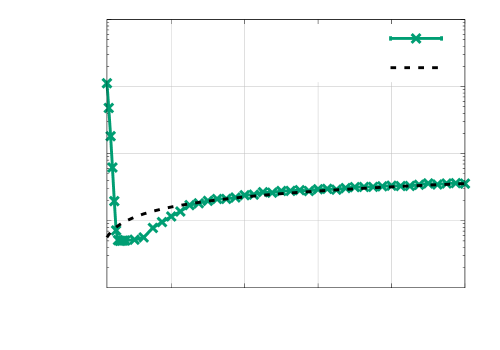
versus the dimension of the DEIM approximation is plotted in Figure 1a. The results indicate a fast decay of the DEIM approximation error with the dimension .
Let us now consider noisy evaluations of the function . Therefore, let be a random vector that has, as components, independent zero-mean Gaussian random variables with standard deviation . Define
| (9) |
so that the DEIM approximation using the noisy function evaluations eq. 9 is
The plot in Figure 1b shows the averaged relative state error
| (10) |
for replicates of the DEIM approximation that is derived from the noisy function evaluations eq. 9 with realization of the noise. The error bars indicate the minimum and maximum of the error over the replicates. Note that the error bars are barely visible, which means the variation over the replicates is small. The results indicate a stability issue of DEIM in this case of noisy function evaluations because the error grows with the dimension of the reduced space. The result illustrates an error growth with a rate with the dimension . Similar observations are made in [2].
Remark 2.1.
The term “instability” has various meanings in numerical analysis. In the following, the term “instability” refers to the specific phenomenon that the DEIM approximation error in the Euclidean norm grows with the dimension of the reduced space if noisy function evaluations (9) (or noisy measurements in the context of state field approximation in Section 2.2) are used; see Figure 1b.
3 Amplification of noise in DEIM
We provide an upper bound on the amplification of the noise in DEIM approximations, and a theoretical explanation of the numerical observation in Figure 1b. The bound eq. 12, which we prove in the following, shows that the error cannot increase faster than with rate , which is the rate observed in Figure 1b. We also provide a formula for the expected value of the DEIM error vector and reveal the structure of the error ellipsoid. A similar bound as eq. 12 has been presented in [2].
To simplify the exposition, we drop the dependence on the state and the parameter of , and abbreviate it as . Similarly, the DEIM approximant will be abbreviated as . The noisy counterparts of and are and , respectively, where is a zero-mean Gaussian vector with independent components with standard deviation .
Lemma 3.1.
Define the error of the DEIM approximation from noisy function evaluations as and the error of the approximation with noise-free function evaluations as . Then, the expected value of the error corresponding to noisy function evaluations equals , i.e., , where the expectation is taken over the noise. The standard deviation of satisfies
| (11) |
Thus, the error is bounded in expectation as
| (12) |
Proof.
Using the linearity of the expectation, the error formula for the DEIM projection, and the assumptions on the noise, namely, , we obtain
| (13) | ||||
which establishes as claimed. The norm of is bounded as
| (14) |
which is the same upper bound as in (5) for the noise-free case. The covariance matrix of the error is
| (15) | |||||
where with being the standard deviation of the -th component of . The covariance is positive semidefinite. Its nonzero eigenvalues (that correspond to the invariant space spanned by ) can be enumerated so that
This is an application of the Ostrowski theorem [25, Theorem 4.5.9]; it identifies the bounds of the amplification factors ’s of the corresponding standard deviations. The spectral structure of (and thus the error ellipsoid) can be explicitly revealed using the SVD (, orthogonal matrices of singular vectors, diagonal matrix of singular values), which yields .
Remark 3.2.
3.1 assumes that the noise is a zero-mean Gaussian vector with independent components. If does not have independent components, i.e., if the noise error covariance matrix is not diagonal, we can write the spectral decomposition of its submatrix as where . Using this spectral decomposition, we replace (15) with
where . Since is an orthogonal matrix, and . Then, the rest of the proof of 3.1 follows as before by replacing with and with , for . Finally, the upper bounds (11) and (12) hold true by replacing with the vector , where now ’s are the variances along the principal components (eigenvectors of ). Moreover, in both (11) and (12), the term can be replaced with .
Corollary 3.3.
Remark 3.4.
Note how in eq. 12, with increasing column dimension of the matrix , the POD projection error monotonically decreases toward zero and, at the same time, the norm of the sampling operator approaches one, while the contribution of the noise grows as , taking over the leading term. The effect of the noise dominating the error is seen in Figure 1.
Remark 3.5.
From 3.1, it follows that it is desirable that a DEIM selection operator avoids components of with noise with high variance. Such a strategy may help slow the noise buildup. If we denote by undesirable indices and set , then we can run the QDEIM selection on the submatrix ; for details we refer the reader to [18, §3.].
4 Stability of GappyPOD with randomized samples
Given the reduced basis matrix , the DEIM selects interpolation points, i.e., is a square matrix. In this section, we investigate oversampling in the sense that more sampling points than the dimension of the reduced space spanned by the columns of are used. Taking more sampling points than the dimension of the space goes under the name of gappy proper orthogonal decomposition (GappyPOD), which has been introduced in [21] and is used in the context for model reduction in [3, 4]. We now show that with GappyPOD, the noise amplification that was observed in Section 3 can be avoided in expectation with high probability if sampling points are randomized and if more sampling points than basis vectors are used.
4.1 GappyPOD
Consider , pairwise distinct sampling points with , i.e., the number of sampling points is larger than the dimension of the space spanned by the columns of the basis matrix . Then, the corresponding GappyPOD approximation of is
where denotes the Moore-Penrose inverse of , i.e., , assuming has linearly independent columns. In contrast to the DEIM approximation in eq. 4, the GappyPOD approximation is obtained via regression and therefore does not necessarily interpolate at the sampling points . In the case of noise-free sampling, the error of the GappyPOD approximation in the Euclidean norm satisfies (see, e.g., [46, Proposition 2.1])
| (17) |
where quantifies the effect of the sampling points and relates to the approximation quality of the space spanned by ; cf. the DEIM error bound eq. 5.
4.2 Probabilistic analysis of GappyPOD
We now investigate the error of the GappyPOD approximation when the sampling points are selected uniformly with replacement from . Note that the following analysis is developed for uniform sampling with replacement as in the work by Balzano et al. [5]. Parts of the following analysis are an application of the work by Cohen et al. [17].
To set up the analysis, we define the coherence of a subspace as
where the columns of form an orthonormal basis for and is the -th row of , see, e.g., [11, Definition 1.2]. Intuitively speaking, coherence measures if there are certain coordinate directions that carry significantly more information than other directions. Note that . The following result from [5, Lemma 3] will be used in our analysis.
Lemma 4.1.
Let the points be uniformly sampled from with replacement and let be the corresponding sampling points matrix. Moreover, let such that and set . Then
with probability at least .
The following lemma states that can be bounded by a constant, arbitrarily close to , with high probability if a sufficiently large number of sampling points is used, which means that GappyPOD with randomized samples is well-posed with high probability.
Lemma 4.2.
Consider the same setup as in 4.1 and set . If is such that, for ,
| (18) |
then
with probability at least .
Proof.
Since
holds, 4.1 yields that with probability at least
| (19) |
Then, the task is to choose so that . To that end, set . By the assumption of 4.1, and thus . The desired inequality becomes
The smaller root of the above parabola is negative and the larger one, then, provides the desired lower bound eq. 18. ∎
The following bound will be helpful in establishing the main result.
Lemma 4.3.
Consider the same setup as in 4.1. Let , and let be the acute angle between and the range of . Then,
| (20) |
with probability at least , where the expected value is with respect to the uniform distribution of the sampling points.
Proof.
We first apply submultiplicativity to obtain
| (21) |
Using eq. 19 and 4.1, we have, with probability at least , that
| (22) |
Consider now the expected value and note that we use the squared Euclidean norm . Let denote the -th component of for . Also let denote the indicator function that is if and 0 otherwise. Note that the probability that is because a uniform distribution with replacement is used for selecting the sampling points, and thus . Then,
| (23) |
Applying Jensen’s inequality to eq. 23 yields which, combined with eq. 22 implies
| (24) |
proving the upper bound in eq. 20 for the first input of the function. To prove eq. 20 for the second input of the function, we first apply submultiplicativity to obtain
| (25) |
With 4.1, we have, with probability at least , that
| (26) |
Let denote the Euclidean inner product and consider the expected value . Using the linearity of and , we obtain
| (27) |
Note that, for , by independence of the th and the th drawing with replacement
| (28) |
Now we can use eq. 28 to split (27). For , we obtain
The remaining terms with contribute to (27) with
where we use for and 0 otherwise. Altogether, we have
| (29) |
where and is the diagonal matrix with the components of on its diagonal. Hence, applying Jensen’s inequality to (29) and then using eq. 26 yields
Combining this final inequality with eq. 24 yields the desired result (20). ∎
Remark 4.4.
The function in the upper bound eq. 20 results from using two different upper bounds for , one as in eq. 21 and the other one as in eq. 25. The latter is employed by [5] for the special case where is orthogonal to the range of . A technical calculation shows that while the first input in the function is expected to be the smaller of the two for small , the second input is expected to be the smaller one for large .
Remark 4.5.
We now show that GappyPOD is robust with respect to noise in the sense that increasing the number of sampling points reduces the effect of the noise.
Theorem 4.6.
Proof.
We split the error following the strategy of [17, Theorem 2]. With the triangular inequality, we obtain
| (32) |
with and .
To bound the first term on the right-hand side of the inequality eq. 32, set . Similarly to the case in [15], it holds that
| (33) |
where we used the fact that with probability, at least, . Note that is orthogonal to the range of . Then, 4.3 implies that
| (34) |
with probability at least . Then, eq. 33 and the linearity of the expectation yield
| (35) |
where is as defined in eq. 30. Now consider the second term on the right-hand side of eq. 32. Note that is not necessarily orthogonal to , and therefore Remark 4.5 cannot be applied. We make the approximations
| (36) |
which holds with probability at least , see eq. 25 and eq. 26 in the proof of 4.3. Consider now . With the same notation as in the proof of 4.3, and building on the proof of [17, Theorem 3], we have
Using the fact that , we obtain
Applying Jensen’s inequality, together with eq. 36 yields
with probability at least . Combining this with eq. 35 proves the theorem. ∎
Remark 4.7.
4.6 reveals that as (recall we perform uniform sampling with replacement), the upper bound in eq. 31 converges to the projection error . In the numerical results in Section 6, rather than investigating the asymptotic behavior as , we will typically keep the ratio low by increasing with and so preventing that the noise term in (31) dominates.
5 The GappyPOD+E deterministic sampling strategy
In this section, we present a deterministic strategy that selects sampling points to reduce the quantity , which controls how sensitive the GappyPOD oblique projection is to perturbations and noise, cf. Section 2.3. While our probabilistic analysis in Section 4 shows that sampling points that are selected uniformly in are sufficient for GappyPOD to be robust with respect to noise, the number of uniformly selected sampling points that are required grows with, e.g., the coherence of the space . The following deterministic selection strategy aims to achieve robustness with fewer points than uniform sampling by taking information about the space into account. We refer to the Introduction in Section 1 for references to other sampling strategies.
We propose the GappyPOD+E sampling algorithm that is based on lower bounds of the smallest eigenvalues of certain structured matrix updates introduced in [27] and that is a special case of the approach introduced by Zimmermann et al. in [46]. The “E” in GappyPOD+E stands for “eigenvector”. The goal of the GappyPOD+E sampling algorithm is to select points that minimize . This minimization problem is equivalent to maximizing the smallest singular value of because
where and denote the largest and smallest singular value of the matrix , respectively. The GappyPOD+E algorithm relies on lower bounds of the smallest eigenvalues to select points that maximize by leveraging the eigenvector corresponding to the smallest eigenvalue.
5.1 Singular values after symmetric rank-one updates
Consider the basis matrix and the sampling points matrix111Note that we have changed the notation slightly here and added the subscript to . This will help distinguish the sampling points matrix when new indices are added. that takes samples. Consider now the SVD of
where contains, as its columns, the left-singular vectors, the matrix is a diagonal matrix with the singular values , in descending order, and contains, as its columns, the right-singular vectors. Note that we assume that has full column rank in the following, which can be ensured by initializing GappyPOD+E with, e.g., the QDEIM interpolation points. If we add a sampling point, we obtain
where is the row of that is selected by the new sampling point. Following the work by Zimmermann et al. [46], the change of the singular values of to can be understood via a symmetric rank-one update. We have
The singular values of are given by the square roots of the eigenvalues of , which we represent as
Define . With , we obtain , which is a symmetric rank-one update to the diagonal matrix . The square roots of the eigenvalues of are the singular values of .
5.2 Lower bounds for eigenvalues of updated matrices
We now use the results by Ipsen et al. in [27] to derive a heuristic strategy with the aim of selecting sampling points that lead to a fast increase of the smallest eigenvalue, i.e., to a fast decrease of .
Let be the eigengap. Note that we need in the following. Let be the eigenvector of corresponding to the smallest eigenvalue , with . In our case is the -th canonical unit vector of dimension because is diagonal with diagonal elements ordered descending. Then, as shown in [27, Corollary 2.2],
| (37) |
Observe that the bound eq. 37 depends on the eigenvector corresponding to the smallest eigenvalue.
The bound eq. 37 motivates us to add the rows of that maximize
| (38) |
The criterion eq. 38 is related to the criteria developed in [46]. While we build on the perturbation bounds introduced in [27], the authors of [46] directly derive criteria that take the eigenvector corresponding to the smallest eigenvalue into account, see [46, page A2834] and [46, Remark 2, item 3]. In fact, the work [46] goes a step further and also takes into account inner products with eigenvectors corresponding to larger eigenvalues. We do not consider these additional steps discussed in [46] in the following.
5.3 The GappyPOD+E algorithm
The GappyPOD+E sampling approach that we consider is summarized in Algorithm 1. It iteratively selects new sampling points that maximize eq. 38 in a greedy fashion. In line 2 of Algorithm 1, the first points are selected with QDEIM, see LABEL:alg:qdeim. Then, for each point , the SVD of (which is U(p, :) in the notation used in Algorithm 1) is computed to obtain the right-singular vectors as columns of the matrix . The eigengap is computed on line 6 in Algorithm 1. Then, is obtained on line 7 in Algorithm 1. The bound (38) is then computed from for each column in lines 8–9 and sorted descending on line 10. On line 9, it is exploited that the eigenvector is the -th canonical unit vector of dimension and so in (38) for column of is computed as , where is the right-singular vector corresponding to the smallest singular value. This means that is given by the last row of (denoted as Ub(end, :) in Algorithm 1). The point corresponding to the column of (row of ) with the largest value (38) is added as sampling point and the procedure is repeated. Each iteration in GappyPOD+E requires performing an SVD of a small matrix whose size grows with the reduced dimension and the number of sampling points. Each SVD is in (for ). Thus, selecting points with GappyPOD+E is in . Note that the sampling point selection is performed during the construction of the reduced model in the offline phase.
The GappyPOD+E algorithm returns points that are not necessarily nested with respect to the dimension of the DEIM basis: Consider a basis matrix with columns and the corresponding set of points selected by GappyPOD+E. Let now be a basis matrix with columns where the first columns coincide with the columns of and let be the set of at least points selected with GappyPOD+E. Then, it is possible that , which is in contrast to, e.g., the greedy EIM algorithm [7], for which holds if and points are selected, respectively. Nestedness of points is a desired property in situations where one wants to, for example, rapidly and adaptively select the number of DEIM basis vectors and sampling points without running the sampling algorithm from scratch. One such situation is in model reduction when the dimension of the DEIM space is selected during the online phase. One option to avoid running GappyPOD+E during the online phase in this situation is to pre-compute GappyPOD+E sampling points for a range of dimensions of the DEIM space and to store them during the offline phase. In the online phase, the pre-computed points can be quickly loaded depending on the basis dimension that is selected online, instead of running GappyPOD+E during the online phase.
6 Numerical results
This section compares the stability of DEIM and GappyPOD with randomized and deterministic sampling algorithms on numerical examples. Section 6.1 revisits the toy example from Section 2.3 and demonstrates that GappyPOD provides stable approximations compared to DEIM. Section 6.2 approximates velocity fields from noisy measurements of single-injector combustion processes following the procedure introduced in [43, 10]. Section 6.3 demonstrates the effect of taking more sampling points than basis vectors on a diffusion-reaction problem, where GappyPOD provides stable approximations in contrast to DEIM.
6.1 Synthetic example
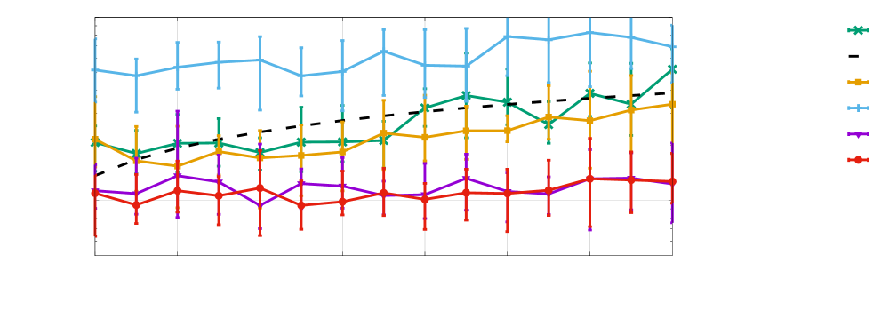
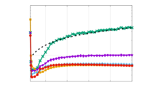
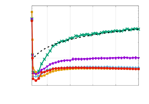
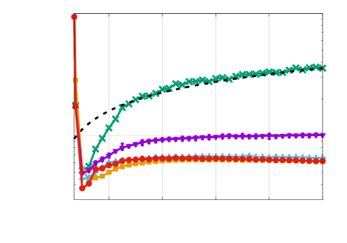
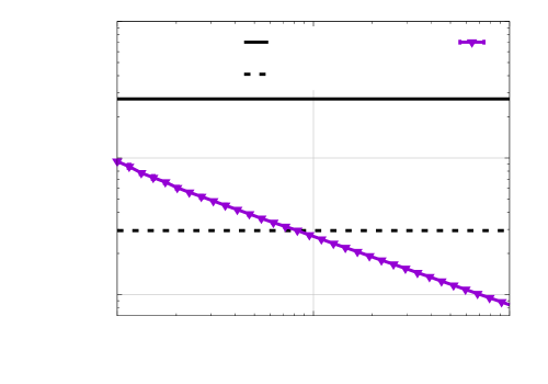
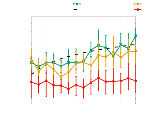
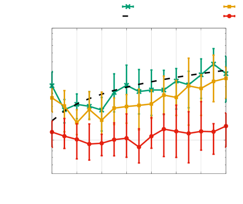
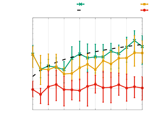
Let us revisit the synthetic example introduced in Section 2.3. We use the same setup as before but now approximate the noisy function with GappyPOD that takes more sampling points than basis vectors. We compare our GappyPOD+E sampling strategy to three sampling strategies from the literature. First, there is GappyPOD+R, which takes the first sampling points with QDEIM and the subsequent sampling points uniform randomly with replacement. Thus, the “R” in GappyPOD+R stands for “random”. Second, the strategy GappyPOD+L takes the first points with QDEIM and the subsequent points based on leverages scores as described in, e.g., [3, Section V.B]. Thus, the “L” in GappyPOD+L stands for “leverage scores”. Third, with GappyPOD+D we denote the sampling strategy introduced in [14, Algorithm 4] that selects sampling points by extending the DEIM greedy algorithm [6, 15]. Thus, the “D” in GappyPOD+D stands for “DEIM greedy”. The number of sampling points is set to in case of GappyPOD in the following. We perform 10 replicates of the experiments and compute the error as defined in eq. 10. The results in Figure 2a indicate that GappyPOD with more sampling points than basis vectors avoids the unstable behavior obtained with DEIM, as suggested by our analysis presented in Section 4. All sampling algorithms perform well in this example, with GappyPOD+E, GappyPOD+L, GappyPOD+D achieving the lowest errors. Similar results are obtained for in this example as shown in Figure 2b-e. Note that the error decays linearly with as long as the noise limits the overall accuracy rather than the projection error, as indicated by Theorem 4.6. The error bars in Figure 2 show the minimum and maximum of the error over the 10 replicates. Except for GappyPOD+R in Figure 2a near , the error bars are barely visible in the plots, which indicates that even small perturbations due to noise lead to unstable behavior in QDEIM.
 |
|
| (a) std. deviation | |
 |
 |
| (b) std. deviation | (c) std. deviation |
 |
 |
| (d) std. deviation | (e) std. deviation |
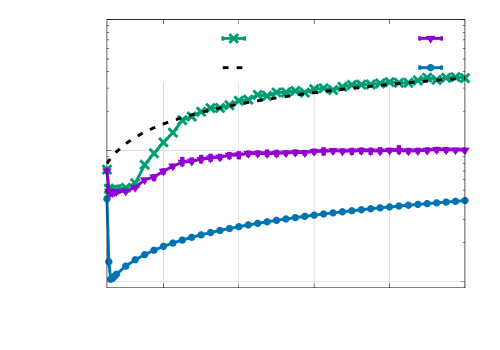
Figure 3a compares the orthogonal projection error of the noisy data,
| (39) |
to error (10) of QDEIM and GappyPOD+R. Note that the projection error (39) grows with the dimension since the Gaussian random noise vector can be better and better approximated in the subspace spanned by the columns of as the dimension is increased. Figure 3b shows that if the dimension is fixed and the number of sampling points is increased, then the error (10) of GappyPOD+R decays with a rate to the projection error of noise-less data, i.e,,
| (40) |
which is below machine precision in this example for . The results shown in Figure 3b are in alignment with Theorem 4.6, which states that the error of GappyPOD with uniform sampling with replacement converges with rate to the projection error.
 |
 |
|---|---|
| (a) sampling with ratio | (b) dimension fixed |
6.2 Velocity field approximations from noisy measurements of single-injector combustion process
We consider velocity field approximations from noisy measurements of the single-injector combustion process described in detail in [40]. The combustion model follows the implementation of the General Equation and Mesh Solver (GEMS) code [24, 26] developed by Purdue University. The domain of the setup of [40] is shown in Figure 4. Fuel and oxidizer are input with constant mass flow rates of and , respectively. The fuel is composed of gaseous methane and the oxidizer is 42% gaseous and 58% gaseous . Details of the physics of the problem setup are described in [26].

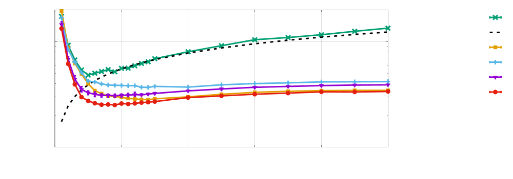
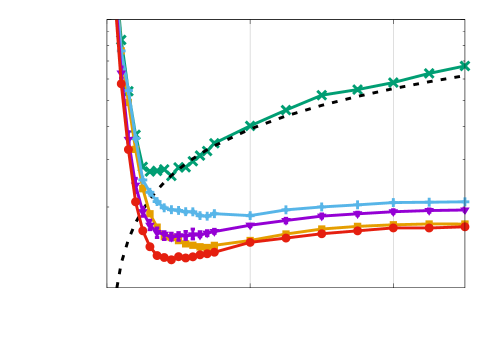
To generate snapshot data, the GEMS code is used to simulate the system for 0.7ms with a time step size of . The simulation leads to 7000 snapshots at 7000 time points . The snapshots are of length (there are 38523 spatial discretization points) and contain the velocity in x and y directions. The basis matrix is derived with POD from the snapshots, where every fourth snapshot is skipped and kept as a test snapshot. Thus, the basis matrix is constructed from 5250 snapshots that are the columns of and the 1750 test snapshots are ignored during construction of the basis matrix and collected as columns in . The test snapshots are polluted with zero-mean Gaussian noise with standard deviation and , respectively, and collected in the noisy test snapshot matrix . A standard deviation of corresponds to about 0.5% noise with respect to the mean of the snapshot matrix. Correspondingly, means that about 1% noise is added to the test snapshots. Figure 5a shows for the relative state error
| (41) |
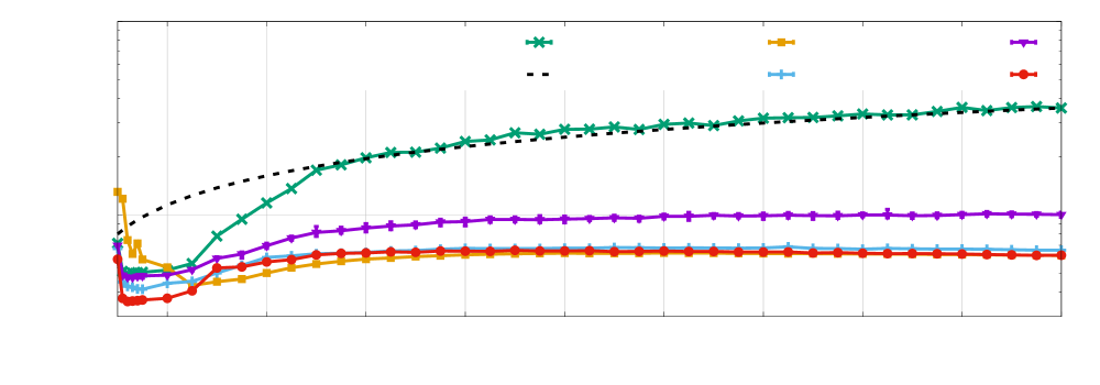
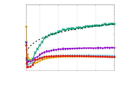
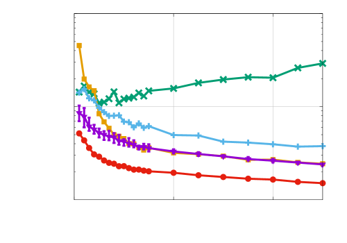
over replicates of noise . The matrix is derived from QDEIM with and from GappyPOD+D, GappyPOD+L, GappyPOD+R, GappyPOD+E, respectively, with , i.e., twice as many sampling points as number of basis vectors. Figure 5a shows the growth of the error (41) for QDEIM, which uses the same number of sampling points as basis vectors. In contrast, taking more sampling points than basis vectors with GappyPOD yields a stable approximation. All sampling strategies help to reduce the error (41) significantly, where GappyPOD+E achieves the lowest error in this example. Error bars show the minimum and the maximum of the error over the replicates. The error bars are barely visible in Figure 5a, which indicates that small perturbations can lead to unstable behavior in QDEIM and that GappyPOD with more sampling points than basis vectors robustly gives stable approximations. Similar results are obtained for in Figure 5b. Figure 5c shows that the norm of the sampling operator is lowest for GappyPOD+E, which is in agreement with the results in Figure 5a and Figure 5b.
 |
|
| (a) std. deviation (about noise) | |
 |
 |
| (b) std. deviation (about noise) | (c) norm of sampling operator |
6.3 Diffusion-reaction problem with nonlinear reaction term
We now demonstrate the stability of GappyPOD and DEIM on a reduced model of a diffusion-reaction problem. The example demonstrates that instabilities in the DEIM approximations can lead to unstable reduced models, which can be avoided with GappyPOD if more sampling points than basis vectors are used.
6.3.1 Problem setup
Let and consider the PDE
| (42) |
where is the spatial coordinate, is the solution function, and is a nonlinear function
with parameter . The PDE eq. 42 is closed with homogeneous Dirichlet boundary conditions. This example is a modification of the example considered in [23].
We discretize eq. 42 with a second-order finite difference scheme on an equidistant mesh with mesh width in , which leads to the state dimension . The system of nonlinear equations is solved with Newton’s method. We derive a reduced model from 1600 snapshots corresponding to a grid of parameter values in the domain . The grid is equidistant in the first direction and logarithmically equidistant in the second direction. The basis matrix is constructed with POD. The POD dimension is chosen as . The nonlinear term is approximated with empirical interpolation, with more details to follow below. The reduced model is tested on parameters corresponding to the grid in that is linearly equidistant in the first direction and logarithmically equidistant in the second direction. The full-model states corresponding to the test parameters are collected in the test snapshot matrix .
6.3.2 Results
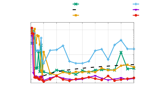
We compare reduced models that differ in the way the nonlinear term is approximated. With “QDEIM” we denote the reduced models that approximate the nonlinear terms with QDEIM, which takes sampling points. Reduced models that approximate the nonlinear term with GappyPOD are denoted as “GappyPOD+D”, “GappyPOD+R”, “GappyPOD+L”, and “GappyPOD+E”, respectively, depending on which sampling strategy is used.
 |
 |
|---|---|
| (a) (factor 4 oversampling) | (b) (factor 8 oversampling) |
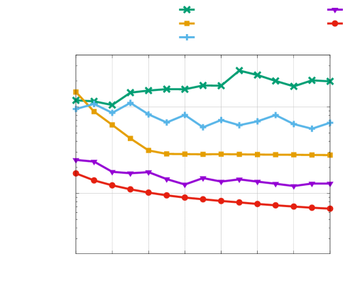
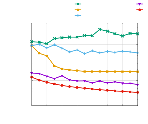
Figure 6 compares the norm of the sampling operators for and for dimensions . GappyPOD+E provides the sampling operator with the lowest norm in this example. We first run the reduced models for the test parameters without adding noise and collect the corresponding states as columns in the matrix where S is either QDEIM, GappyPOD+D, GappyPOD+L, GappyPOD+R, or GappyPOD+E. The averaged relative state error
| (43) |
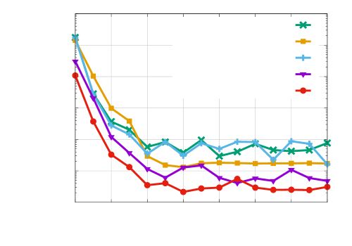
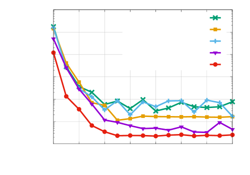
is shown in Figure 7a for an oversampling factor and in Figure 7b for for S either QDEIM, GappyPOD+D, GappyPOD+L, GappyPOD+R, or GappyPOD+E. QDEIM as well as GappyPOD with all sampling strategies achieve stable approximations in the sense described in Section 2.3, i.e., the error (43) does not grow with the dimension of the reduced space.
 |
 |
| (a) oversampling | (b) oversampling |
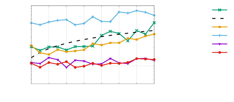
We now run the reduced models for the test parameters and perturb the nonlinear function evaluations with zero-mean Gaussian noise and standard deviation . We repeat this process times and collect the states of a reduced model corresponding to the test parameters as columns in for . Then, the averaged relative state error
| (44) |
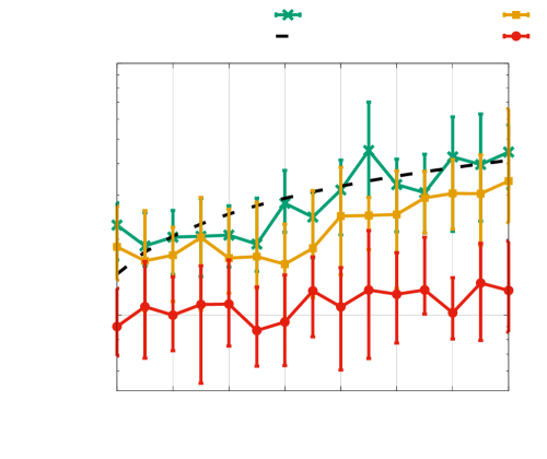
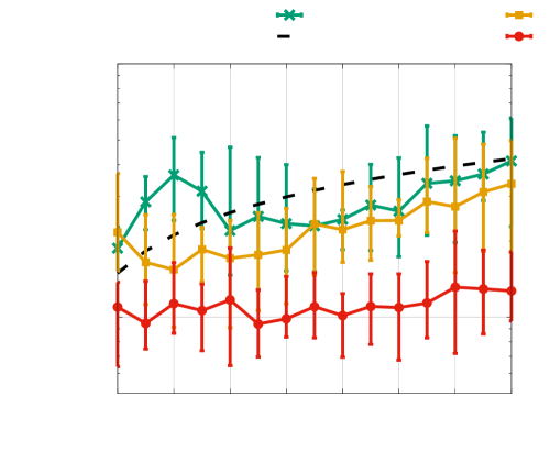
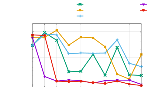
is reported in the following for each reduced model. Figure 8 compares the error (44) for reduced models based on QDEIM, GappyPOD+D, GappyPOD+L, GappyPOD+R, and GappyPOD+E. The standard deviation of the noise is and the oversampling factor is 4, i.e., . The growth of the error (44) with rate can be observed for QDEIM in Figure 8. Similarly, the reduced models based on GappyPOD+D seem unstable because the corresponding errors grow with a rate of too. In contrast, GappyPOD+E and GappyPOD+R give stable reduced models, where the error does not increase with the dimension of the reduced space spanned by the columns of . The curves plotted in Figure 8 are shown in Figure 11 with error bars that indicate the minimum and maximum error over the replicates. The sampling points selected with GappyPOD+L lead to models with poor performance in this example even though the growth of the error with rate cannot be observed in the plot in Figure 8. However, the error bars shown in Figure 11 for GappyPOD+L are larger than for the other sampling algorithms, which indicates that there is strong variability in the approximation error achieved with GappyPOD+L in this example. The strong variability with respect to accuracy of the selected points might hide the growth of the error. Figure 9 compares GappyPOD+E with QDEIM and GappyPOD+D for oversampling factors and and standard deviations . The error bars show the minimum and maximum error over the replicates. In all cases, GappyPOD+E leads to a stable reduced model in the sense that the error does not grow with the dimension of the DEIM space, whereas QDEIM and GappyPOD+D show unstable behavior and a growth of the error with rate .
 |
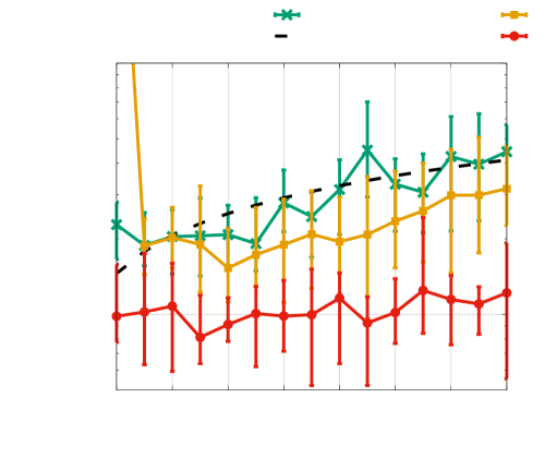 |
| (a) std. deviation , oversampling | (b) std. deviation , oversampling |
 |
 |
| (c) std. deviation , oversampling | (d) std. deviation , oversampling |
 |
 |
| (e) std. deviation , oversampling | (f) std. deviation , oversampling |
 |
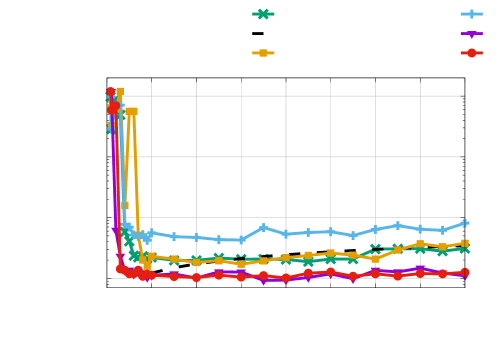 |
| (a) std. deviation | (b) std. deviation |
 |
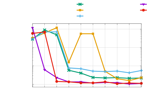 |
| (c) detail of plot (a) | (d) detail of plot (b) |
Consider now Figure 10 that shows results for POD dimension , which is lower than dimension used previously. The POD space of dimension preserves about 99.9% of the energy, a typical threshold used in model reduction; cf. [8, Section 3.1.1]. Note that the energy is where are the singular values of the snapshot matrix in descending order. The standard deviation of the noise is set to and , respectively. The mean over 10 runs is shown in Figure 10. Similar behavior in terms of error as for higher POD dimensions is observed. Plot (c) in Figure 10 shows a detail of (a) and indicates that the approximations based on GappyPOD+R and GappyPOD+E have less oscillatory error than approximations obtained with QDEIM, GappyPOD+L, and GappyPOD+D for DEIM dimensions between 5 and 50 in this example.
Remark 6.1.
We comment on the problem setup: In this example, we considered nonlinear function evaluations that are perturbed with noise. We might encounter such a situation if, for example, parameters of the nonlinear function first need to be estimated from data via a Bayesian approach that introduces noise into the function evaluations used in the reduced model. Our analysis does not cover deterministic approximation errors stemming from, e.g., relaxed tolerances of iterative solvers, and thus it remains future work to show if our analysis applies to such general types of noise as well.
7 Conclusions
Empirical interpolation is widely used for approximating nonlinear terms in reduced models and for recovering state fields from few spatial measurements; however, stability issues have been observed in presence of noise and other perturbations. Our probabilistic analysis shows that the particular instability that arises due to perturbations such as noise can be provably avoided by employing GappyPOD and taking more sampling points than dimensions of the reduced space. Numerical results demonstrated that instabilities in DEIM can lead to a loss of accuracy in the reduced model outputs and that randomized and deterministic sampling strategies together with GappyPOD give stabler approximations.
Acknowledgements
The authors thank Karthik Duraisamy (University of Michigan), Cheng Huang (University of Michigan), and David Xu (University of Michigan) for providing the snapshots corresponding to the single-injector combustion process discussed in Section 6.2.
References
- [1] J.-P. Argaud, B. Bouriquet, F. de Caso, H. Gong, Y. Maday, and O. Mula, Sensor placement in nuclear reactors based on the generalized empirical interpolation method, Journal of Computational Physics, 363 (2018), pp. 354 – 370.
- [2] J. P. Argaud, B. Bouriquet, H. Gong, Y. Maday, and O. Mula, Stabilization of (G)EIM in presence of measurement noise: Application to nuclear reactor physics, in Spectral and High Order Methods for Partial Differential Equations ICOSAHOM 2016, M. L. Bittencourt, N. A. Dumont, and J. S. Hesthaven, eds., Cham, 2017, Springer International Publishing, pp. 133–145.
- [3] P. Astrid, S. Weiland, K. Willcox, and T. Backx, Missing point estimation in models described by proper orthogonal decomposition, in Decision and Control, 2004. CDC. 43rd IEEE Conference on, vol. 2, Dec 2004, pp. 1767–1772 Vol.2.
- [4] P. Astrid, S. Weiland, K. Willcox, and T. Backx, Missing point estimation in models described by proper orthogonal decomposition, IEEE Transactions on Automatic Control, 53 (2008), pp. 2237–2251.
- [5] L. Balzano, B. Recht, and R. Nowak, High-dimensional matched subspace detection when data are missing, in 2010 IEEE International Symposium on Information Theory, June 2010, pp. 1638–1642.
- [6] M. Barrault, Y. Maday, N. Nguyen, and A. Patera, An “empirical interpolation” method: Application to efficient reduced-basis discretization of partial differential equations, Comptes Rendus Mathématique. Académie des Sciences. Paris, I (2004), pp. 339–667.
- [7] M. Barrault, N. C. Nguyen, Y. Maday, and A. T. Patera, An empirical interpolation method: Application to efficient reduced-basis discretization of partial differential equations, C. R. Acad. Sci. Paris, Série I., 339 (2004), pp. 667–672.
- [8] P. Benner, S. Gugercin, and K. Willcox, A survey of projection-based model reduction methods for parametric dynamical systems, SIAM Review, 57 (2015), pp. 483–531.
- [9] P. Binev, A. Cohen, O. Mula, and J. Nichols, Greedy algorithms for optimal measurements selection in state estimation using reduced models, SIAM/ASA Journal on Uncertainty Quantification, 6 (2018), pp. 1101–1126.
- [10] T. Bui-Thanh, M. Damodaran, and K. Willcox, Aerodynamic data reconstruction and inverse design using proper orthogonal decomposition, AIAA journal, 42 (2004), pp. 1505–1516.
- [11] E. J. Candès and B. Recht, Exact matrix completion via convex optimization, Foundations of Computational Mathematics, 9 (2009), p. 717.
- [12] K. Carlberg, Model reduction of nonlinear mechanical systems via optimal projection and tensor approximation, PhD thesis, Stanford University, 2011.
- [13] K. Carlberg, C. Bou-Mosleh, and C. Farhat, Efficient non-linear model reduction via a least-squares Petrov–Galerkin projection and compressive tensor approximations, International Journal for Numerical Methods in Engineering, 86 (2011), pp. 155–181.
- [14] K. Carlberg, C. Farhat, J. Cortial, and D. Amsallem, The GNAT method for nonlinear model reduction: Effective implementation and application to computational fluid dynamics and turbulent flows, Journal of Computational Physics, 242 (2013), pp. 623–647.
- [15] S. Chaturantabut and D. Sorensen, Nonlinear model reduction via discrete empirical interpolation, SIAM Journal on Scientific Computing, 32 (2010), pp. 2737–2764.
- [16] Chkifa, Abdellah, Cohen, Albert, Migliorati, Giovanni, Nobile, Fabio, and Tempone, Raul, Discrete least squares polynomial approximation with random evaluations - application to parametric and stochastic elliptic PDEs, ESAIM: M2AN, 49 (2015), pp. 815–837.
- [17] A. Cohen, M. A. Davenport, and D. Leviatan, On the stability and accuracy of least squares approximations, Foundations of Computational Mathematics, 13 (2013), pp. 819–834.
- [18] Z. Drmač and S. Gugercin, A new selection operator for the Discrete Empirical Interpolation Method – improved a priori error bound and extensions, SIAM Journal on Scientific Computing, 38 (2016), pp. A631–A648.
- [19] Z. Drmač and A. Saibaba, The discrete empirical interpolation method: Canonical structure and formulation in weighted inner product spaces, SIAM Journal on Matrix Analysis and Applications, 39 (2018), pp. 1152–1180.
- [20] J. L. Eftang and B. Stamm, Parameter multi-domain ’hp’ empirical interpolation, International Journal for Numerical Methods in Engineering, 90 (2012), pp. 412–428.
- [21] R. Everson and L. Sirovich, The Karhunen-Loeve Procedure for Gappy Data, Journal of the Optical Society of America, 12 (1995), pp. 1657–1664.
- [22] F. Ghavamian, P. Tiso, and A. Simone, POD-DEIM model order reduction for strain-softening viscoplasticity, Computer Methods in Applied Mechanics and Engineering, 317 (2017), pp. 458–479.
- [23] M. A. Grepl, Y. Maday, N. C. Nguyen, and A. T. Patera, Efficient reduced-basis treatment of nonaffine and nonlinear partial differential equations, ESAIM: Mathematical Modelling and Numerical Analysis, 41 (2007), pp. 575–605.
- [24] M. E. Harvazinski, C. Huang, V. Sankaran, T. W. Feldman, W. E. Anderson, C. L. Merkle, and D. G. Talley, Coupling between hydrodynamics, acoustics, and heat release in a self-excited unstable combustor, Physics of Fluids, 27 (2015), p. 045102.
- [25] R. A. Horn and C. R. Johnson, Matrix Analysis, Cambridge University Press, New York, NY, USA, 2nd ed., 2012.
- [26] C. Huang, K. Duraisamy, and C. Merkle, Investigations and improvement of robustness of reduced-order models of reacting flow, in AIAA Scitech 2019 Forum, AIAA, 2019.
- [27] I. C. F. Ipsen and B. Nadler, Refined perturbation bounds for eigenvalues of Hermitian and Non-Hermitian matrices, SIAM Journal on Matrix Analysis and Applications, 31 (2009), pp. 40–53.
- [28] Y. Maday and O. Mula, A generalized empirical interpolation method: Application of reduced basis techniques to data assimilation, in Analysis and Numerics of Partial Differential Equations, F. Brezzi, P. Colli Franzone, U. Gianazza, and G. Gilardi, eds., Springer, 2013, pp. 221–235.
- [29] Y. Maday, O. Mula, A. Patera, and M. Yano, The generalized empirical interpolation method: Stability theory on Hilbert spaces with an application to the Stokes equation, Computer Methods in Applied Mechanics and Engineering, 287 (2015), pp. 310–334.
- [30] K. Manohar, B. W. Brunton, J. N. Kutz, and S. L. Brunton, Data-Driven Sparse Sensor Placement for Reconstruction, ArXiv e-prints, (2017).
- [31] K. Manohar, S. L. Brunton, and J. N. Kutz, Environment identification in flight using sparse approximation of wing strain, Journal of Fluids and Structures, 70 (2017), pp. 162 – 180.
- [32] G. Migliorati, F. Nobile, and R. Tempone, Convergence estimates in probability and in expectation for discrete least squares with noisy evaluations at random points, Journal of Multivariate Analysis, 142 (2015), pp. 167 – 182.
- [33] B. Peherstorfer, Model reduction for transport-dominated problems via online adaptive bases and adaptive sampling, arXiv:1812.02094, (2018).
- [34] B. Peherstorfer, D. Butnaru, K. Willcox, and H. Bungartz, Localized discrete empirical interpolation method, SIAM Journal on Scientific Computing, 36 (2014), pp. A168–A192.
- [35] B. Peherstorfer and K. Willcox, Online adaptive model reduction for nonlinear systems via low-rank updates, SIAM Journal on Scientific Computing, 37 (2015), pp. A2123–A2150.
- [36] B. Peherstorfer, K. Willcox, and M. Gunzburger, Survey of multifidelity methods in uncertainty propagation, inference, and optimization, SIAM Review, 60 (2018), pp. 550–591.
- [37] S. B. Pope, Simple models of turbulent flows, Physics of Fluids, 23 (2011), p. 011301.
- [38] G. Rozza, D. Huynh, and A. Patera, Reduced basis approximation and a posteriori error estimation for affinely parametrized elliptic coercive partial differential equations, Archives of Computational Methods in Engineering, 15 (2007), pp. 1–47.
- [39] S. Sargsyan, S. L. Brunton, and J. N. Kutz, Nonlinear model reduction for dynamical systems using sparse sensor locations from learned libraries, Phys. Rev. E, 92 (2015), p. 033304.
- [40] R. Swischuk, B. Kramer, C. Huang, and K. Willcox, Learning physics-based reduced-order models for a single-injector combustion process, AIAA Journal, 0 (2020), pp. 1–15. (accepted).
- [41] H. Weyl, Das asymptotische verteilungsgesetz der eigenwerte linearer partieller differentialgleichungen (mit einer anwendung auf die theorie der hohlraumstrahlung), Mathematische Annalen, 71 (1912), pp. 441–479.
- [42] J. H. Wilkinson, The Algebraic Eigenvalue Problem, Oxford University Press, 1988.
- [43] K. Willcox, Unsteady flow sensing and estimation via the gappy proper orthogonal decomposition, Computers & Fluids, 35 (2006), pp. 208 – 226.
- [44] Y. B. Zhou, Model reduction for nonlinear dynamical systems with parametric uncertainties, PhD thesis, Massachusetts Institute of Technology, 2012.
- [45] R. Zimmermann, B. Peherstorfer, and K. Willcox, Geometric subspace updates with applications to online adaptive nonlinear model reduction, SIAM Journal on Matrix Analysis and Applications, 39 (2018), pp. 234–261.
- [46] R. Zimmermann and K. Willcox, An accelerated greedy missing point estimation procedure, SIAM Journal on Scientific Computing, 38 (2016), pp. A2827–A2850.
Appendix A Additional listings and figures
