Bayesian Modular and Multiscale Regression

Abstract

We tackle the problem of multiscale regression for predictors that are spatially or temporally indexed, or with a pre-specified multiscale structure, with a Bayesian modular approach. The regression function at the finest scale is expressed as an additive expansion of coarse to fine step functions. Our Modular and Multiscale (M&M) methodology provides multiscale decomposition of high-dimensional data arising from very fine measurements. Unlike more complex methods for functional predictors, our approach provides easy interpretation of the results. Additionally, it provides a quantification of uncertainty on the data resolution, solving a common problem researchers encounter with simple models on down-sampled data. We show that our modular and multiscale posterior has an empirical Bayes interpretation, with a simple limiting distribution in large samples. An efficient sampling algorithm is developed for posterior computation, and the methods are illustrated through simulation studies and an application to brain image classification. Source code is available as an R package at github.com/mkln/bmms.

Keywords: Bayesian, functional regression, Haar wavelets, high-dimensional data, large p small n, modularization, multiresolution

1 Introduction

Modern researchers routinely collect very high-dimensional data that are spatially and/or temporally indexed, with the intention of using them as inputs in regression-type problems. A simple example with a binary output is time-series classification; analogously, brain images can be used as diagnostic tools. In these cases, prediction of the outcome variable and interpretation of the results are the main goals, but obtainining clear interpretation and accurate prediction simultaneously is notoriously difficult. In fact, adjacent measurement locations tend to be highly correlated, with possibly huge numbers of measurements at a very high resolution.

In these settings, directly inputing such data into usual regression methods leads to poor results. In fact, methods for dimensionality reduction that do not take advantage of predictor structure can have poor performance in estimating regression coefficients and sparsity patterns when the dimension is huge and predictors are highly correlated (see e.g. Figure 1). Theoretical guarantees in such settings typically rely on strong assumptions on sparsity, low linear dependence, and high signal-to-noise (Zhao and Yu, 2006; Wasserman and Roeder, 2009; Bühlmann and van de Geer, 2011, Chapter 7; Scarlett and Cevher, 2017).

Figure 1: Brain regions parcellated according to Gordon et al., (2016) and selected in a Lasso model for a gender classification task.

The above problems can be alleviated by down-sampling the data to lower resolutions before analysis. This is an appealing option because of the potential for huge dimensionality reduction. However, any specific resolution choice might be perceived as ad-hoc, and hide patterns at different scales that could instead be highlighted by a multiresolution approach. This problem cannot be solved by methods that somewhat take into account predictor structure, but only act on a single measurement scale, like the group Lasso of Yuan and Lin, (2006), the fused Lasso of Tibshirani et al., (2005), the Bayesian method of Li and Zhang, (2010), and data-driven projection approaches such as PCR (Delaigle and Hall,, 2012).

Alternatively, one can use methods for “functional predictors” (Ramsay and Silverman,, 1997; Morris,, 2015; Reiss et al.,, 2017), which view time- or spatially-indexed predictors as corresponding to realizations of a function. Typically this involves estimating a time or spatially-indexed coefficient function, which is assumed to be represented as a linear combination of basis functions. Specifically, multiscale interpretations are achievable via wavelet bases. However, a discrete wavelet transform of the data will not reduce its dimensionality, making down-sampling a necessary pre-processing step for the estimation of Bayesian wavelet regression (see e.g. Brown et al., 2001). Additionally, wavelets require the basis functions to be orthogonal; this leads to benefits in terms of identifiability and performance in estimating the individual coefficients, while also leading to disadvantages relative to “over-complete” specifications. In fact, wavelets cannot be used when there is uncertainty on multiple pre-specified resolutions that do not conform to a wavelet decomposition (e.g. a hour/day/week structure for time-series). This is also true for ongoing research in neuroscience devoted to the development of parcellation schemes that achieve reproducible and interpretable results (Thirion et al.,, 2014; Schiffler et al.,, 2017). Researchers might be interested in using these scales jointly in a regression model to ascertain their relative contribution, but this cannot be achieved with wavelets. For classical references on wavelet regression, see Donoho and Johnstone, (1994, 1995); Zhao et al., (2012); from a Bayesian perspective, see e.g. Brown et al., (2001) or Jeong et al., (2013).

To solve these issues, we propose a class of Bayesian Modular and Multiscale regression methods (BM&Ms), which express the regression function as an additive expansion of functions of data at increasing resolutions. In its simplest form, the regression function becomes an additive expansion of coarse to fine step functions. This implies that multiple down-samplings of the predictor are included within a single flexible multiresolution model. Our approach can be used when (1) there is a pre-determined multiscale structure, or uncertainty on a multiplicity of pre-specified resolutions, as in the case of brain atlases; (2) with temporally- or spatially-indexed predictors, when the goal is a multiscale interpretation of single-scale data. In the first case, our method can be directly used to ascertain the contribution of the pre-determined scales to the regression function. This goal cannot be achieved via wavelets. In the second case, BM&Ms are related to a Haar wavelet expansion but involve a simpler, non-orthogonal transformation that facilitates easy interpretation, and suggests a straightforward extension to scalar-on-tensor regression. We address the identifiability issues induced by this non-orthogonal expansion by taking a modularization approach. The resulting BM&M regression is stable, well identified, easily interpretable, and provides uncertainty quantification at different resolutions.

The idea of modularization in Bayesian inference is that instead of using a fully Bayesian joint probability model for all components of the model, one “cuts” the dependence between different components or modules (see Liu et al., (2009); Jacob et al., (2017) and references therein). Modularization has been commonly applied in joint modeling contexts for computational and robustness reasons. For example, suppose that one defines a latent factor model for multivariate predictors $X$, with the goal of using factors $\eta$ in place of $X$ in a model for the response $Y$. Under a coherent fully Bayes model, $Y$ will impact the posterior on $\eta$. This is conceptually appealing in providing some supervision under which one may infer latent factors that are particularly informative about $Y$. However, it turns out that there is a lack of robustness to model misspecification, with misspecification potentially leading to inferring factors that are primarily driven by improving fit of the model and are not interpretable as summaries of $X$. Modularization solves this problem by not allowing $Y$ to influence the posterior of $\eta$; motivated by the practical improvements attributable to such an approach, WinBUGS has incorporated a cut(.) function to allow cutting of dependence in routine Bayesian inference (Plummer,, 2015).

Our multiscale setting is different than previous work on Bayesian modularization, in that we use modules to combine information from the same data at increasingly higher resolutions. Chen and Dunson, (2017) recently proposed a modular Bayesian approach for screening in contexts involving massive-dimensional features, but there was no multiscale structure, allowance for functional predictors, or consideration of multiple predictors that simultaneously impact the response.

Section 2 introduces BM&Ms in a general setting, highlighting the correspondence to a data-dependent prior in a coherent Bayesian model. Section 3 focuses on linear regression. Section 4 outlines an algorithm to sample from the modular posterior. Section 5 contains applications on simulated data and to a brain imaging classification task. Proofs and technical details are included in an Appendix.

2 A modular approach for multiscale regression

We consider a regression problem linking a scalar response $y_{i}$ to an input vector $\mathbf{x}_{i}=(x_{s,i})_{s\in S}$ of dimension $p\gg n$, for each subject $i\in\{1,\dots,n\}$. For example, a subject’s health outcome may be linked to the output from a high-resolution recording device. The goal is to predict the outcome variable and explain its variability across subjects by identifying specific patterns in the sensor recording at different resolutions.

We denote the vector of responses by $y$ and the raw data matrix by $X_{S}$. Each row of $X_{S}$ can be down-sampled to get a new design matrix $X_{S_{j}}$, where $S_{j}$ is a lower resolution grid such that $|S_{j}|<|S|$. Down-sampling can be achieved by summing or averaging adjacent columns, or subsetting them. We simplify the notation slightly by calling $X=X_{S}$ and $X_{j}=X_{S_{j}}$. We consider the same data at increasing resolutions in an additive model:

$$y=f_{0}(X_{0})+\dots+f_{j}(X_{j})+\dots+f_{K}(X_{K})+\varepsilon,$$ (1)

where $f_{j}$ is the resolution $j$ contribution to the regression function. With this additive multiresolution expansion, it is difficult to disambiguate the impact of the coarse scales from the finer ones, leading to identifiability issues. One may be able to fit $y$ using only a fine scale component, with the coarse scales discarded. If we were to attempt fully Bayes inferences by placing priors on the different component functions, large posterior dependence would lead to substantial computational problems (e.g. very poor mixing of Markov chain Monte Carlo algorithms) and it would not be possible to reliably interpret the different $f_{j}$s. This happens in particular if each $f_{j}$ is linear, as seen in Section 3.

We bypass these problems by adopting a modular approach (Liu et al.,, 2009; Jacob et al.,, 2017), splitting the overall joint model (1) into components or modules which are kept partly separate from each other, to get a modular posterior. In the following, for $j>i$ we use the notation $A_{i:j}=\{A_{i},\dots,A_{j}\}$.

Definition 2.1.

Within the overall model (1), module j for data at resolution $S_{j}$ consists of a prior for $f_{j}$, and a model for $y|f_{1:j}$:

$$f_{j}|f_{1:j-1}\sim\pi(f_{j}|f_{1:j-1})\qquad y|f_{j},f_{1:j-1}\sim p_{j}(y|f_{j},f_{1:j-1})$$

where model $p_{j}$ estimates $f_{j}$ via $y=f_{1}(X_{1})+\dots+f_{j-1}(X_{j-1})+f_{j}(X_{j})+\varepsilon_{j}$, and $f_{1},\dots,f_{j-1}$ are considered known. The output from module $j$ is the (conditional) posterior for $f_{j}$ obtained by prior $\pi(f_{j})$ and model $p_{j}$, and we denote it by $m(f_{j}|f_{1:j-1})$:

$$m(f_{j}|f_{1:j-1})=\frac{\pi(f_{j}|f_{1:j-1})p_{j}(y|f_{1:j},X_{1:j})}{p_{j}(y|f_{1:j-1},X_{1:j})}.$$ (2)

Thus for the full model (1) we build $K$ modules, using increasingly higher resolution data, with each module being a refinement on previous output.

Definition 2.2.

The modular prior distribution for $\mathbf{f}=(f_{1},\dots,f_{K})$ corresponds to $p_{M}(\mathbf{f})=\pi(f_{1})\cdots\pi(f_{j}|f_{1:j-1})\cdots\pi(f_{K}|f_{1:K-1})$, whereas the modular posterior distribution $p_{M}(\mathbf{f})$ is:

$$p_{M}(\mathbf{f}|y,X_{1:K}) =m(f_{1})m(f_{2}|f_{1})\cdots m(f_{K}|f_{1:K-1}),$$

thus collecting the posteriors in (2). Each module refines the output from previous modules by using higher resolution data, and the modular posterior is obtained by aggregating all refinements. Modularity is evidenced by resolution dependence, which is only allowed downwardly, as opposed to letting it be bidirectional as in a fully Bayes approach.

Proposition 2.1.

There exists a data-dependent prior $\pi_{d}$ and a likelihood $p_{d}$ such that $p_{M}(\mathbf{f}|y,X)\propto\pi_{d}(\mathbf{f})p_{d}(y|\mathbf{f},X)$. Specifically, $p_{d}(\cdot)$ is the likelihood corresponding to model $y=f_{1}(X_{1})+f_{2}(X_{2})+\varepsilon$, and the data-dependent prior is $\pi_{d}(\mathbf{f})=\pi(f_{1})\pi(f_{2}|f_{1})\frac{p_{1}(f_{1}|y,X_{1})}{p_{2}(f_{1}|y,X_{1:2})}$.

Proof.

See Appendix B. ∎

The above proposition implies our modular approach to multiscale regression will resemble a fully Bayesian model if $\frac{p_{1}(f_{1}|y,X_{1})}{p_{2}(f_{1}|y,X_{1:2})}\approx 1$, i.e. if the modules agree on the marginal posterior probability of $f_{1}$, the low resolution contribution to the regression function.

3 BM&Ms for linear regression

We now assume that $f_{j}=X_{j}\theta_{j}$ and our goal is to study $\theta_{j}$ for $j=1,\dots,K$ in the model

$$y=X_{1}\theta_{1}+\dots+X_{K}\theta_{K}+\varepsilon_{K},$$ (3)

where $\varepsilon_{K}\sim N(0,\sigma^{2}_{K})$. The model includes data up to resolution $S_{K}$. We also assume that $X_{j}=X_{j+1}L_{j}=X_{K}\mathcal{L}_{j}$, meaning that $L_{j}$ and $\mathcal{L}_{j}$ respectively down-sample $X_{j+1}$ and $X_{K}$ to $X_{j}$. This allows us to decompose $\beta_{K}$, the usual regression coefficient of $y$ on $X_{K}$ as:

$$y=X_{K}\left(\mathcal{L}_{1}\theta_{1}+\dots+\mathcal{L}_{K}\theta_{K}\right)+\varepsilon_{K}=X_{K}\beta_{K}+\varepsilon_{K},$$ (4)

thus interpreting $\theta_{j}$ as the contribution of resolution $S_{j}$ to the regression function.

However, model (3) is ill-posed, leading to problems with standard techniques for model fitting. In fact, the effective design matrix $X=[X_{1}\cdots X_{K}]$ is such that $det(X^{\prime}X)=0$, as the columns of $X_{j}$ are linear combinations of columns of $X_{j+1}$. One can potentially obtain a well defined posterior through an informative prior for ${\theta}$. However, this posterior will be highly dependent on the prior, as the likelihood has many flat regions.

We solve this problem via modularization as in section 2. The modular posterior is

$$p_{M}({\theta}|y,X_{1:K}) =\frac{\pi(\theta_{1})p_{1}(y|\theta_{1},X_{1})}{p_{1}(y|X_{1})}\cdots\frac{\pi(\theta_{K}|\theta_{1:K-1})p_{K}(y|\theta_{1:K},X_{1:K})}{p_{K}(y|\theta_{1:K-1},X_{1:K})},$$

where $p_{j}(\cdot)$ is the likelihood for the response $y$ under $y=\sum_{h=1}^{j}X_{h}\theta_{h}+\varepsilon_{j}$, $\varepsilon_{j}\sim N(0,\sigma^{2}_{j})$, and $\theta_{1},\dots,\theta_{j-1}$ are considered known. The posterior distribution for the coarsest scale coefficient $\theta_{1}$ is derived treating all the finer scale coefficients as equal to zero; this makes $\theta_{1}$ identifiable and interpretable as producing the best coarse scale approximation to the regression function. In defining the posterior for $\theta_{2}$, we then condition on $\theta_{1}$ and set coefficients $\theta_{3},\ldots,\theta_{K}$ equal to zero, and so on. Linearity allows us to write $p_{j}(\cdot)$ as

$$y-\sum_{h=1}^{j-1}X_{h}\theta_{h}=X_{j}\theta_{j}+\varepsilon_{j},\quad\text{ }\quad\varepsilon_{j}\sim N(0,\sigma^{2}_{j}),$$

which essentially means that we are estimating $\theta_{j}$ (and $\sigma^{2}_{j}$) using the residuals $e_{j-1}=y-\sum_{h=0}^{j-1}X_{h}\theta_{h}$ from the previous modules as responses for the current module. Hence, the modular posterior for (3) is built using simpler, well-identified single-scale models as modules. For example, we address uncertainty on two resolutions with the following model:

$$y=X_{1}\theta_{1}+X_{2}\theta_{2}+\varepsilon_{2},\quad\text{ }\quad\varepsilon\sim N(0,\sigma^{2}_{2}I_{n}),$$ (5)

assigning priors $\theta_{j}\sim N(m_{j},\sigma^{2}_{j}M_{j})$, $\sigma^{2}_{j}\sim\text{InvG}(a,b)$ for $j\in\{1,2\}$, and using a first module corresponding to model $y=X_{1}\theta_{1}+\varepsilon_{1}$ with $\varepsilon_{1}\sim N(0,\sigma^{2}_{1}I_{n})$.

Proposition 3.1.

The modular posterior of $\theta|\sigma^{2}_{1},\sigma^{2}_{2}$ for model (5) is $N\left(\mu_{1:2},\Sigma_{1:2}\right)$ where

$$\begin{array}[]{ccc}\mu_{1:2}=\begin{bmatrix}\mu_{1}\\ \mu_{2}\end{bmatrix}=\begin{bmatrix}\mu_{\beta_{1}}\\ \mu_{\beta_{2}}-Q_{1}\mu_{\beta_{1}}\end{bmatrix}&&\Sigma_{1:2}=\begin{bmatrix}\sigma^{2}_{1}\Sigma_{1}&-\sigma^{2}_{1}\Sigma_{1}Q_{1}^{\prime}\\ -\sigma^{2}_{1}Q_{1}\Sigma_{1}&\sigma^{2}_{2}\Sigma_{2}+\sigma^{2}_{1}Q_{1}\Sigma_{1}Q_{1}^{\prime}\end{bmatrix},\end{array}$$ (7)

with $Q_{1}$ = $\Sigma_{2}X_{2}^{\prime}X_{1}$, and $\mu_{\beta_{j}}=\Sigma_{j}^{-1}(M_{j}m_{j}+X_{j}^{\prime}y)$ for $j\in\{1,2\}$. Proof in Appendix C.1.

Finally, note we can estimate $\beta_{2}$ in $y=X_{2}\beta_{2}+\varepsilon_{2}$ by accumulating all components, i.e. using $L_{1}\theta_{1}+\theta_{2}$, which reconstructs the decomposition in (4).

3.1 Asymptotics of BM&Ms in linear regression

We now assume that $(y,\mathcal{X})$ were generated according to a process such that

$$\frac{1}{n}\begin{bmatrix}y^{\prime}y&y^{\prime}\mathcal{X}\\ \mathcal{X}^{\prime}y&\mathcal{X}^{\prime}\mathcal{X}\end{bmatrix}\xrightarrow[a.s.]{}\begin{bmatrix}\omega_{yy}&\mathbf{\omega}_{y\mathbf{x}}\\ \mathbf{\omega}_{\mathbf{x}y}&\Omega\end{bmatrix},$$

a positive definite matrix, and $y|\mathcal{X},\sigma^{2}\sim N(\mathcal{X}b,\sigma^{2}I_{n})$, where $b\in\mathbb{R}^{p}$ with dimension not depending on the sample size. We consider a two-scale linear model like in (5). We assume $X_{2}=\mathcal{X}\mathcal{L}_{2}$, $X_{1}=X_{2}L_{1}$, and assign priors on $\theta_{j}$ that have positive density on $\mathbb{R}^{p_{j}}$. Finally, we assume $\sigma^{2}_{j}$ is known for each module.

Proposition 3.2.

The modular posterior distribution of $(\theta_{1},\theta_{2})$ in model $y=X_{1}\theta_{1}+X_{2}\theta_{2}+\varepsilon$ is approximated by $N(\bar{\mu}_{1:2},\bar{\Sigma}_{1:2})$, where

$$\begin{array}[]{ccc}\bar{\mu}_{1:2}=\begin{bmatrix}\theta_{1}^{*}\\ \theta_{2}^{*}\end{bmatrix}=\begin{bmatrix}\beta_{1}^{*}\\ \beta_{2}^{*}-L_{1}\beta_{1}^{*}\end{bmatrix}&&\bar{\Sigma}_{1:2}=\begin{bmatrix}\sigma^{2}_{1}\Omega_{1}^{-1}&-\sigma^{2}_{1}\Omega_{1}^{-1}L_{1}^{\prime}\\ -\sigma^{2}_{1}L_{1}\Omega_{1}^{-1}&\sigma^{2}_{2}\Omega_{2}^{-1}+\sigma^{2}_{1}L_{1}\Omega_{1}^{-1}L_{1}^{\prime}\end{bmatrix}\end{array}$$

where $\beta_{j}^{*}$ is the pseudo-true value of $b$ under the model $y=X_{j}\beta_{j}+\varepsilon$.

Proof.

See Appendix C.2. ∎

This is also the asymptotic distribution of $(\hat{\theta}_{1},\hat{\theta}_{2})$, where $\hat{\theta}_{1}=\hat{\beta}_{1}$ and $\hat{\theta}_{2}$ is the least-squares estimator obtained by regressing $y-X_{1}\hat{\beta}_{1}$ on $X_{2}$. Hence, in large samples, BM&Ms correspond to a sequential least squares procedure that regresses the residuals of coarser models on higher resolution data. Our approach propagates uncertainty across multiple stages on finite samples, unlike many two-stage procedures (see e.g. Murphy and Topel, (1985) for a treatment of two-stage estimators in econometrics).

Corollary 3.1.

The large sample distributions of $\theta_{1}$ and $L_{1}\theta_{1}+\theta_{2}$ are approximated by $N(\beta_{1}^{*},\frac{\sigma^{2}_{2}}{n}\Omega_{1}^{-1})$ and $N(\beta_{2}^{*},\frac{\sigma^{2}_{2}}{n}\Omega_{2}^{-1})$, respectively. In other words, accumulating the modular posterior mean components up to $j$ results in a consistent and asymptotically efficient estimator for $\beta_{j}^{*}$.

Proof.

This is a direct consequence of the properties of the Normal distribution. ∎

4 Computation of the modular posterior

We sample from the modular posterior of 2.2 by sequentially sampling from each module.

for $t\in\{1,\dots,T\}$ do

       Start: Draw sample $f_{1}^{(t)}$ from the module $1$ posterior $m(f_{1})=p_{1}(f_{1}|y,X_{1})$

       for $j\in\{2,\dots,K\}$ do

             Draw sample $f_{j}^{(t)}$ from the module $j$ posterior

$$m(f_{j}|f_{1:j-1}^{(t)})=p_{j}(f_{j}|f_{1:j-1}^{(t)},y,X_{1:j})=p_{M}(f_{j}|\mathbf{f}_{-j},y,X_{1:K})$$ (8)

       end for

      

end for

Algorithm 1 Sampling $\left\{\mathbf{f}^{(t)}\right\}_{t\in\{1,\dots,T\}}$ from the modular posterior $p_{M}(\mathbf{f}|y,X_{K})$

Obtaining a sample from the modular posterior depends on $m(f_{j}|f_{1:j-1}^{(t)})$, which is determined by the module choice. Therefore, in a multiscale linear regression with conjugate priors as in section 3 we can easily sample from each individual module taking advantage of Eq. (7). In the more complex cases where $m(f_{j}|f_{j-1}^{(t)})$ is approximated via MCMC, we can use the fact that for all $j$, $p_{j}(f_{j}|f_{1:j-1},y,X_{1:j-1})=p_{M}(f_{j}|f_{-j},y,X_{1:K})$, i.e. the posterior distribution of each module corresponds to the full conditional distribution of the overall modular model, hence sampling from a module’s posterior can be seen as a “modular” Gibbs step. This also means that the computational complexity of BM&Ms is of the same order of magnitude of each component module, since $K$ is taken to be small.

5 Applications

5.1 Simulation study

We generate $n=60$ observations from a linear regression model $y=X\beta+\varepsilon$, with

$$\begin{matrix}\varepsilon\sim N(0,I_{n})&\quad&\Omega=(\omega_{h,j})\quad h,j=1,\dots,p&\quad&p=128&\\ \mathbf{x}_{i}\sim N(0,\Omega)&\quad&\omega_{h,j}=\exp\{-(1-\rho)|h-j|\}&\quad&\rho=0.98\end{matrix}$$

and where $\beta$ is a $p\times 1$ vector obtained by discretizing the Doppler, Blocks, HeaviSine, Bumps, and Piecewise Polynomial functions of Donoho and Johnstone, (1994, 1995); Nason and Silverman, (1994) on a regular grid. Notice that covariates are highly correlated, and the sample size is relatively low, suggesting that the regression function may be challenging to estimate at a fine resolution. Our goals are thus: (1) dimension reduction and multiscale decomposition of $\beta$; (2) estimation and uncertainty quantification of the relative contributions of different scales; (3) out-of-sample prediction. The $k^{\text{th}}$ module, given $\theta_{k-1}$, is specified by $y_{k}=X\theta_{k}+\varepsilon_{k}$, with $\varepsilon_{k}\sim N(0,\sigma^{2}_{k})$, $y_{k}=y_{k-1}-X\theta_{k-1}$ and $\theta_{k}=(\theta_{k,1},\cdots,\theta_{k,p})^{\prime}$ with

$$\theta_{k,j} =\begin{cases}b_{1},&\text{if}\ 0<j\leq t_{1}\\ \dots\\ b_{H_{k}},&\text{if}\ t_{H_{k}-1}<j\leq t_{H_{k}}=p\end{cases}$$ (9)

the goal being estimation of $b_{1},\dots,b_{H_{k}}$ and the split locations $t_{1},\dots,t_{H-1}$. We use 3 modules and fix $H_{1}=1,H_{2}=2,H_{3}=4$. This allows us to estimate an unknown, hierarchical, 3-scale decomposition of $\beta$. MCMC approximations of the modular posterior decomposition of $\beta$ in the Heavi and Blocks cases are in Figure 2.

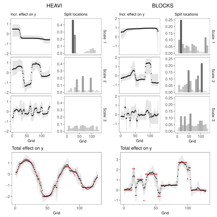
Figure 2: Model-averaged BM&Ms decomposition of $\beta$. The total effect is the sum of the intermediate scale contributions. In red, the true unknown $\beta$. For Heavi, Scale 3 has little to no contribution to the overall estimation, as evidenced by the 95% credible bands including 0. For Blocks, Scale 3 refines on the previous ones in a few select locations.

Within the above setup, BM&Ms compare favorably to the other models in almost all cases (Figure 3), owing to an (implicit) multiscale structure (Doppler, Blocks), and/or non-smoothness (Blocks, Bumps).

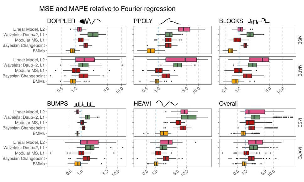
Figure 3: Mean Square Error in estimating $\beta$, and Mean Absolute Prediction Error on 100 samples of size $n_{\text{out}}=100$, relative to Fourier regression on the same data (blue dashed line).

5.2 Gender differences in multiresolution tfMRI data

Brain activity and connectivity data plays a central role in neuroscience research today, but increasingly higher-resolution medical imaging devices make management and analysis of such data challenging. We use data from the Human Connectome Project (HCP) (Essen et al.,, 2013; Glasser et al.,, 2013), considering a sample of $n=100$ subjects, with the goal of classifying subjects’ genders using brain activation data during task-based functional Magnetic Resonance Imaging (tfMRI). Gender differences have been observed in neuroscience and linked to brain morphology and connectivity (Tomasi and Volkow,, 2012; Gong et al.,, 2011), or task-based activity patterns (Kaisera et al.,, 2009; Lee et al.,, 2014). For an overview see Garrett and Hough, (2018, Chapter 7). We use BM&Ms on tfMRI data recorded during the social task in HCP, preprocessed according to the Gordon333 (Gordon et al.,, 2016) parcellation. This hierarchical partitioning splits the brain into a multiscale structure of 333 regions, 26 lobes, and 2 hemispheres.

While we expect each region to have low explanatory power on its own, it is unclear whether grouping them to form a coarser structure might improve predictive power. In particular, while the coarse-scale 26 lobes are easily interpretable given their connection to known brain functions, they might not be an efficient coarsening for our predictive task. We thus implement BM&Ms in two ways, following the two multiscale points of view of Section 1: (1) we consider the regions-lobes multiscale structure as specified by Gordon et al., (2016); (2) we use regions’ centroid information to adaptively collapse them into coarser groups. In both cases, we consider a binary regression model with probit link, and hence assume that $Pr(y_{i}=1)=\Phi\left(\mathbf{x}_{1,i}\theta_{1}+\dots+\mathbf{x}_{K,i}\theta_{K}\right)$, where $y_{i}$ is binary and corresponds to the subject’s gender, and $\mathbf{x}_{j,i}$ is the same subject’s data at resolution $j$.

We adapt the Gibbs sampling algorithm of Albert and Chib, (1993) to BM&Ms . We thus introduce a latent variable $Z_{i}$ for each subject, and alternate sampling from $p(Z_{i}|y_{i},\theta_{1:K},\mathbf{x}_{i,1:K})$ and $p_{M}(\theta_{1:K}|y,Z,X_{1:K})$. Here, $p(Z_{i}|y_{i},\theta_{1:K},\mathbf{x}_{i,1:K})$ is the usual truncated Normal distribution, centered at $\mathbf{x}_{i,1}\theta_{1}+\dots+\mathbf{x}_{i,K}\theta_{K}$, with unit variance, and truncation on zero to the left if $y_{i}=1$, to the right if $y_{i}=0$. On the other hand, $p_{M}$ denotes the modular posterior of a linear model as above.

In implementation (1), $X_{j}$ is a $n\times p_{j}$ matrix collecting subjects’ brain activation data at resolutions $j\in\{1,2\}$ corresponding to regions and lobes, so that $p_{1}=333,p_{2}=26$. We use Bayesian Spike & Slab modules to estimate $\theta_{j}=(\theta_{j,1},\cdots,\theta_{j,p_{j}})$ for $j\in\{1,2\}$. We are interested in estimating the posterior distributions of $\theta_{j}$, and to understand whether lobes provide additional information compared to the baseline of regions. The estimated posterior means are shown at the top of Figure 4. In implementation (2), we fix $K=5$ to decompose the original higher-resolution parcellation. Implementation of each module follows the lines of (9), but using two-dimensional spatial information, as detailed in Appendix D.2. The estimated posterior means are shown at the bottom of figure 4.

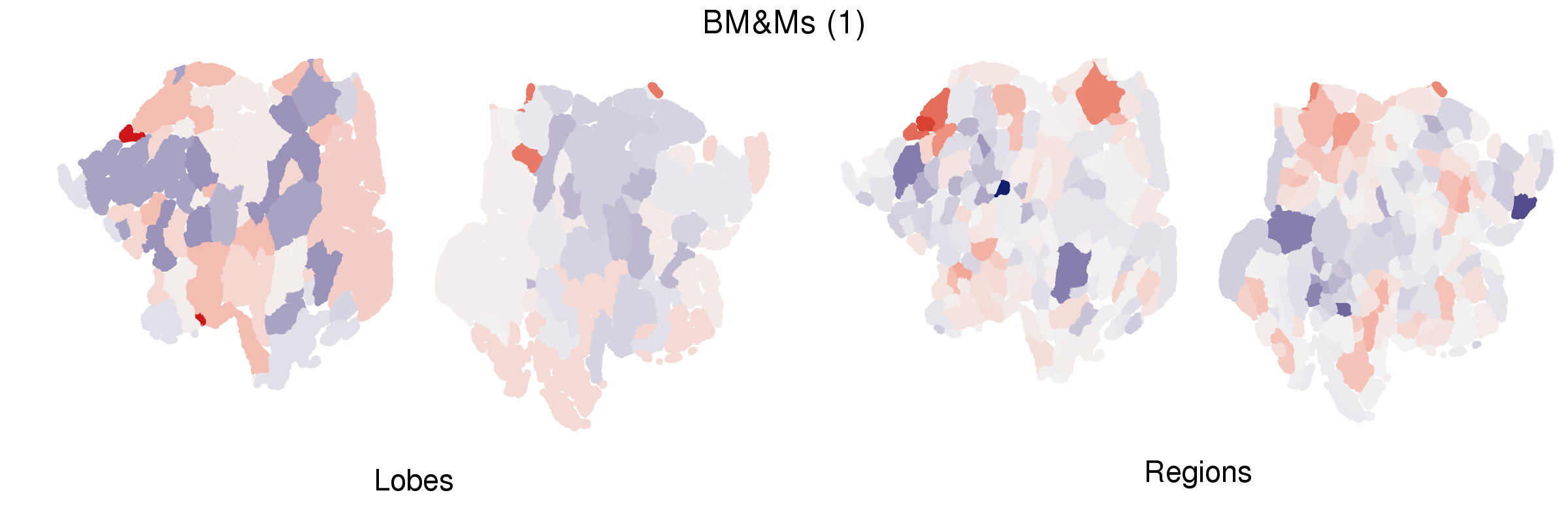
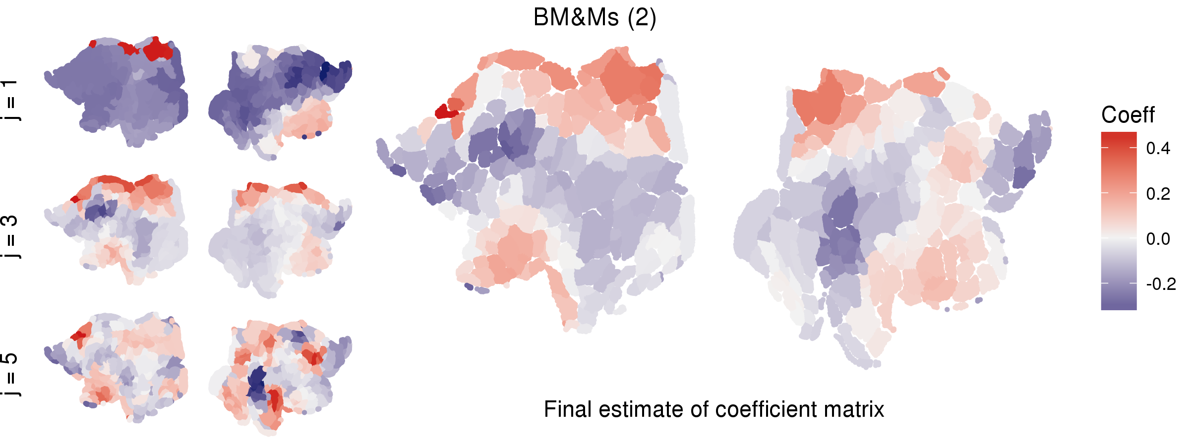
Figure 4: Posterior means estimated with BM&Ms . Top: lobes-regions multiscale structure. Bottom: Multiscale decomposition (left) of an estimated coefficient image (right) in a scalar-on-image regression setting.

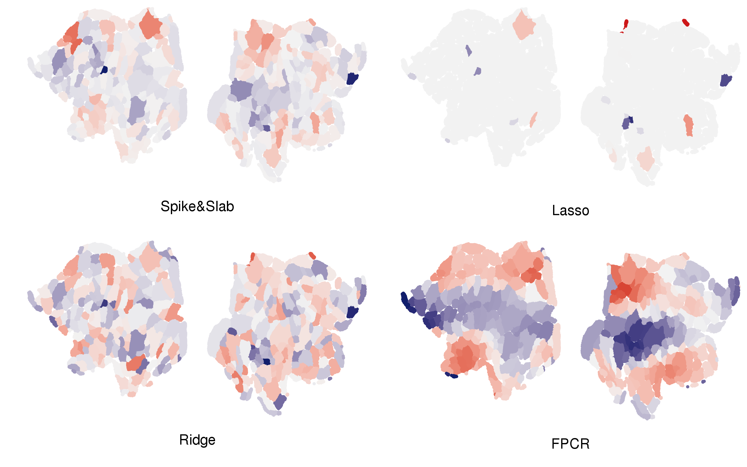
Figure 5: Coefficient on brain regions estimated via four alternative single-scale models.

Model	Accuracy	AUC	Multiscale	Bayesian	Scalar-on-Image
BM&Ms (1)	0.806	0.889	✓	✓
BM&Ms (2)	0.810	0.889	✓	✓	✓
Spike & Slab	0.800	0.883		✓
Ridge	0.792	0.871
Lasso	0.749	0.824
Functional PCR	0.781	0.856			✓

Table 1: Correct classification rate (Accuracy), and area under ROC curve (AUC), on random samples of size $n_{\text{out}}=385$, averaged across 200 resamples of the data.

We compare BM&Ms to competing models on the same data. Table 1 reports the out-of-sample performance of all tested models, whereas Figure 5 shows the estimation output of the competitors. BM&Ms perform at least as well as competing models, while providing additional information on the multiscale structure. On one hand, ridge regression achieves good out-of-sample performance but the resulting estimates prevent a clear understanding of the results. Lasso regression would lead researchers to believe some regions might account for gender differences, yet its performance is the worst among tested models. Spike & Slab priors result in many regions being infrequently selected, and this may lead researchers to believe that coarser scale information from lobes might be useful. However, applying BM&Ms on the regions-lobes multiscale structure results in little to no improvement in predictive power, with lobes being selected rarely. Finally, when considering the spatial structure of the brain regions, the estimated coefficient images of BM&Ms and FPCR are similar. However, the BM&Ms image can be decomposed in coarse-to-fine contributions (shown in Figure 4, bottom left), which aid in the interpretation of the final estimate.

6 Discussion

In this article, we introduced a Bayesian modular approach that builds an overall model by the sequential application of increasingly more complex component modules. Our approach can be applied to multiscale regression problems in two common scenarios: (1) when multiple resolutions of the data could be used to model the regression relationship, to assess their contribution to the regression function; (2) when the focus of analysis is on a multiscale interpretation of results. Compared to established methods for multiscale regression such as wavelets, our method is more flexible and with the potential of easier interpretation. Both simulations and real data analysis show that this is not achieved at the expense of performance.

The modular posterior of BM&Ms is the product of each module’s posterior. This implies that our method inherits properties of the chosen component modules. Choosing component modules requires clarity on what the objective of analysis is. For example, we showed in Section 5 that we can use variable selection modules when the resolution structure is pre-specified, and changepoint-detection modules to find a multiscale interpretation. However, other module choices can be explored for different objectives, and overall models with mixed-type modules might offer additional interpretation opportunities. Additionally, our approach can also be used in non-parametric regression settings by considering the identity matrix $I_{n}$ as the high-resolution design matrix.

Appendix A Notation

$y$	output vector of size $n\times 1$
$S_{j}$	resolution of the data, $j\in\{1,\dots,K\}$
$\mathcal{S}$	unknown “true” resolution
$X_{S_{j}}=X_{j}$	design matrix at resolution $S_{j}$, size $n\times p_{j}$
$\mathcal{X}$	data matrix corresponding to $\mathcal{S}$
$b$	“true” coefficient vector, such that $y=\mathcal{X}b+\varepsilon$
$\mathcal{L}_{j}$	$p\times p_{j}$ matrix such that $\mathcal{X}\mathcal{L}_{j}=X_{j}$
$L_{j}$	$p_{j+1}\times p_{j}$ matrix such that $X_{j+1}L_{j}=X_{j}$
$\beta_{j}$	coefficient vector in single-resolution model $y=X_{j}\beta_{j}+\varepsilon_{j}$
$\mu_{\beta_{j}}$	posterior mean for $\beta_{j}$ in the single-resolution model $y=X_{j}\beta_{j}+\varepsilon_{j}$
$\hat{\beta}_{j}$	LS estimate of $\beta_{j}$ in the single-resolution model $y=X_{j}\beta_{j}+\varepsilon_{j}$
$\sigma^{2}_{j}$	variance of $\varepsilon_{j}$
$L_{j}$	coarsening operator such that $X_{j+1}L_{j}=X_{j}$
$\mathcal{L}_{j}$	coarsening operator such that $X_{K}\mathcal{L}_{j}=X_{j}$
$\theta_{j}$	$j$th component of the multiresolution parameter $\theta$
$\theta=(\theta_{1}\cdots\theta_{K})$	multiresolution parameter for a K-resolution model
$\beta_{K}=\mathcal{L}_{1}\theta_{1}+\dots+\mathcal{L}_{K}\theta_{K}$	multiresolution decomposition of the coefficient vector
$N(m_{j},\sigma^{2}_{j}M_{j})$	prior for $\theta_{j}$
$N(\mu_{j},\sigma^{2}_{j}\Sigma_{j})$	posterior for $\theta_{j}$ obtained with module $j$

Appendix B Appendix to Section 2

Proposition B.1.

There exists a data-dependent prior $\pi_{d}$ and a likelihood $p_{d}$ such that $p_{M}(\mathbf{f}|y,X)\propto\pi_{d}(\mathbf{f})p_{d}(y|\mathbf{f},X)$. Specifically, $p_{d}(\cdot)$ is the likelihood corresponding to model $y=f_{1}(X_{1})+f_{2}(X_{2})+\varepsilon$, and the data-dependent prior is $\pi_{d}(\mathbf{f})=\pi(f_{1})\pi(f_{2}|f_{1})\frac{p_{1}(f_{1}|y,X_{1})}{p_{2}(f_{1}|y,X_{1:2})}$.

Proof.

We consider without loss of generality the case with two modules represented by data $X_{1}$ and $X_{2}$, respectively. Here, $p_{1}(\cdot)$ corresponds to the reduced model $y=f_{1}(X_{1})+\varepsilon_{1}$, while $p_{2}(\cdot)$ to $y=f_{1}(X_{1})+f_{2}(X_{2})+\varepsilon$. We build the modular posterior using the modules’ posteriors, and multiply and divide by $p_{2}(y|X_{1:2})$:

$$p_{M}(\mathbf{f}|y,X) =m(f_{1})m(f_{2}|f_{1})=\frac{\pi(f_{1})p_{1}(y|f_{1},X_{1})}{p_{1}(y|X_{1})}\frac{\pi(f_{2}|f_{1})p_{2}(y|f_{1},f_{2},X_{1:2})}{p_{2}(y|f_{1},X_{1:2})}$$

$$=\pi(f_{1})\pi(f_{2}|f_{1})\frac{p_{1}(y|f_{1},X_{1})p_{2}(y|X_{1:2})}{p_{2}(y|f_{1},X_{1:2})p_{1}(y|X_{1})}\frac{p_{2}(y|f_{1},f_{2},X_{1:2})}{p_{2}(y|X_{1:2})}.$$

We thus interpret $\frac{p_{2}(y|f_{1},f_{2},X_{1:2})}{p_{2}(y|X_{1:2})}$ as the likelihood divided by the normalizing constant. This means the modular posterior can be obtained via the full model $y=f_{1}(X_{1})+f_{2}(X_{2})+\varepsilon$ where both $f_{1}$ and $f_{2}$ are unknown, and a prior on $f_{1},f_{2}$ which depends on the data through the following factor:

$$\frac{p_{1}(y|f_{1},X_{1})p_{2}(y|X_{1:2})}{p_{2}(y|f_{1},X_{1:2})p_{1}(y|X_{1})}=\frac{p_{1}(y|f_{1},X_{1})}{p_{1}(y|X_{1})}\cdot\frac{p_{2}(y|X_{1:2})}{p_{2}(y|f_{1},X_{1:2})}=\frac{p_{1}(f_{1}|y,X_{1})}{\pi_{1}(f_{1})}\cdot\frac{p_{2}(y|X_{1:2})}{p_{2}(y|f_{1},X_{1:2})}$$

We then use the fact that according to model $p_{2}$,

$$p_{2}(y|X_{1:2}) =\frac{\pi(f_{1})\pi(f_{2}|f_{1})p_{2}(y|f_{1},f_{2},X_{1:2})}{p_{2}(f_{1},f_{2}|y,X_{1:2})}=\frac{\pi(f_{1})\pi(f_{2}|f_{1})p_{2}(y|f_{1},f_{2},X_{1:2})}{p_{2}(f_{2}|y,X_{1:2},f_{1})p_{2}(f_{1}|y,X_{1:2})}.$$

and hence we obtain that

$$\frac{p_{2}(y|X_{1:2})}{p_{2}(y|f_{1},X_{1:2})}=\frac{\pi(f_{1})}{p_{2}(f_{1}|y,X_{1:2})}\cdot\frac{\pi(f_{2}|f_{1})p_{2}(y|f_{1},f_{2},X_{1:2})}{p_{2}(y|f_{1},X_{1:2})p_{2}(f_{2}|y,X_{1:2},f_{1})}.$$

Since $p_{2}(f_{2}|y,X_{1:2},f_{1})=\frac{\pi(f_{2}|f_{1})p_{2}(y|f_{1},f_{2},X_{1:2})}{p_{2}(y|f_{1},X_{1:2})}$, we can write the modular posterior as

$$p_{M}(\mathbf{f}|y,X) =\pi(f_{1})\pi(f_{2}|f_{1})\frac{p_{1}(f_{1}|y,X_{1})}{p_{2}(f_{1}|y,X_{1:2})}\cdot\frac{p_{2}(y|f_{1:2},X_{1:2})}{p_{2}(y|X_{1:2})}.$$

∎

Appendix C Appendix to Section 3

C.1 Two-scale BM&Ms posterior

The modular posterior of $\theta|\sigma^{2}_{1},\sigma^{2}_{2}$ for the BM&Ms of model (5) is

$$\theta=\begin{bmatrix}\theta_{1}&\theta_{2}\end{bmatrix}^{\prime}\sim N\left(\mu_{1:2},\Sigma_{1:2}\right)$$ (10)

$$\begin{array}[]{ccc}\mu_{1:2}=\begin{bmatrix}\mu_{1}\\ \mu_{2}\end{bmatrix}=\begin{bmatrix}\mu_{\beta_{1}}\\ \mu_{\beta_{2}}-Q_{1}\mu_{\beta_{1}}\end{bmatrix}&&\Sigma_{1:2}=\begin{bmatrix}\sigma^{2}_{1}\Sigma_{1}&-\sigma^{2}_{1}\Sigma_{1}Q_{1}^{\prime}\\ -\sigma^{2}_{1}Q_{1}\Sigma_{1}&\sigma^{2}_{2}\Sigma_{2}+\sigma^{2}_{1}Q_{1}\Sigma_{1}Q_{1}^{\prime}\end{bmatrix}\end{array}$$

where we denote $Q_{1}$ = $\Sigma_{2}X_{2}^{\prime}X_{1}$, and $\mu_{\beta_{j}}$ with $j\in\{0,1\}$ are the posterior means we would obtain from single resolution models of the form

$$y=X_{j}\beta_{j}+\varepsilon_{j},$$ (11)

when we assign prior $\beta_{j}\sim N(m_{j},\sigma^{2}_{j}M_{j})$.

We build module 1, $m(\theta_{1})$ with a prior $\pi(\theta_{1},\sigma^{2}_{1})$ and a model $p_{1}(y|\theta_{1},\sigma^{2}_{1})$:

$$\pi(\sigma^{2}_{1})\propto\frac{1}{\sigma^{2}_{1}} \quad\text{ }\quad\pi(\theta_{1}|\sigma^{2}_{1})=N(m_{1},\sigma^{2}_{1}M_{1})$$

$$p_{1}(y|\theta_{1},\sigma^{2}_{1},X_{1})=N(X_{1}\theta_{1},\sigma^{2}_{1}I_{n})$$

From this we obtain the posterior

$$\begin{array}[]{lcl}p(\theta_{1}|\sigma^{2}_{1},y,X_{1})=N(\mu_{1},\sigma^{2}_{1}\Sigma_{1})&\quad\text{where}&\Sigma_{1}=\left(M_{1}^{-1}+X_{1}^{\prime}X_{1}\right)^{-1}\\ &&\mu_{1}=\Sigma_{1}\left(M_{1}^{-1}m_{1}+X_{1}^{\prime}y\right)\end{array}$$

Conditioning on $\theta_{1}=\tilde{\theta}_{1}$, we then build module 1:

$$\pi(\sigma^{2}_{2})\propto\frac{1}{\sigma^{2}_{2}} \quad\text{ }\quad\pi(\theta_{1}|\sigma^{2}_{2})=N(m_{2},\sigma^{2}_{2}M_{2})$$

$$p_{2}(y|\theta_{1}=\tilde{\theta}_{1},\sigma^{2}_{2},X_{1:2})=N(X_{1}\tilde{\theta}_{1}+X_{2}\theta_{2},\sigma^{2}_{2}I_{n})$$

Hence, the posterior for $\theta_{1}|\theta_{1}$ will be

$$\begin{array}[]{lcl}p(\theta_{1}|\theta_{1}=\tilde{\theta}_{1},\sigma^{2}_{2},y,X_{1:2})=N(\mu_{2},\sigma^{2}_{2}\Sigma_{2})&\quad\text{where}&\Sigma_{2}=\left(M_{2}^{-1}+X_{1}^{\prime}X_{1}\right)^{-1}\\ &&\mu_{2}=\Sigma_{2}\left(M_{2}^{-1}m_{2}+X_{1}^{\prime}(y-X_{1}\tilde{\theta}_{1})\right)\end{array}$$

We find the posterior distribution $\theta$ via modules 0 and 1:

$$\begin{array}[]{ccc}\theta_{1}|\sigma^{2}_{1},y,X_{1}\sim N(\mu_{1},\sigma^{2}_{1}\Sigma_{1})&&\theta_{2}|\theta_{1},\sigma^{2}_{1},\sigma^{2}_{2},y,X_{2}\sim N(\mu_{2},\sigma^{2}_{2}\Sigma_{2})\end{array}$$

The end result follows from the properties of the Normal distribution.

C.2 Asymptotics for BM&Ms

The goal of this section is to show that the modular posterior in linear models is approximately normal in large samples, with a mean that is a composition of the (rescaled) pseudo-true regression coefficients at different resolutions. In order to do so, it will be sufficient to show that each module results in approximately normal (conditional) posteriors. This will ensure normality of the overall modular posterior, by the properties of the normal distribution.

We consider response vector $y$ and data matrix $\mathcal{X}$, and following Geweke, (2005) we assume that $(y,\mathcal{X})$ were generated according to a process such that

$$\frac{1}{n}\begin{bmatrix}y^{\prime}y&y^{\prime}\mathcal{X}\\ \mathcal{X}^{\prime}y&\mathcal{X}^{\prime}\mathcal{X}\end{bmatrix}\xrightarrow[a.s.]{}\begin{bmatrix}\omega_{yy}&\mathbf{\omega}_{y\mathbf{x}}\\ \mathbf{\omega}_{\mathbf{x}y}&\Omega\end{bmatrix},$$

a positive definite matrix, and

$$y|\mathcal{X},\sigma^{2}\sim N(\mathcal{X}b,\sigma^{2}I_{n}),$$

where $b\in\mathbb{R}^{p}$ with dimension not depending on the sample size, and $\sigma^{2}$ is known. We consider a finite set of predetermined resolutions $S_{1},\dots,S_{K}$, corresponding to $X_{1},\dots,X_{K}$, respectively, such that $X_{j}=\mathcal{X}\mathcal{L}_{j}$ and $X_{j+1}L_{j}=X_{j}$ for some $\mathcal{L}_{j}$ and $L_{j}$, $j\in\{1,\dots,K\}$. Here, $\mathcal{L}_{j}$ and $L_{j}$ are coarsening operators that perform partial sums of adjacent columns and hence reduce the data dimensionality to $p_{j}$, from $p$ or $p_{j+1}$, respectively. In other words, we assume $X_{j}$, the data at available resolution $S_{j}$, could be obtained as coarsening of the true-model data $\mathcal{X}$, and that each of the intermediate resolutions can be obtained as coarsening of higher resolutions. Given these assumptions, we have

$$\frac{1}{n}\begin{bmatrix}y^{\prime}y&y^{\prime}X_{j}\\ X_{j}^{\prime}y&X_{j}^{\prime}X_{j}\end{bmatrix}\xrightarrow[a.s.]{}\begin{bmatrix}\omega_{yy}&\mathbf{\omega}_{y\mathbf{x}_{j}}\\ \mathbf{\omega}_{\mathbf{x}_{j}y}&\Omega_{j}\end{bmatrix}.$$

Note that we do not assume $\mathcal{L}_{j}=I_{p}$ necessarily for some $j$. In other words, if $S$ is the resolution of the data corresponding to the true regression coefficient $b$, it may hold that $S_{j}\neq S$ for all $j$. The goal is to find the “best approximation” of $b$ at the different predetermined resolutions.

We consider without loss of generality the overall model

$$y=X_{1}\theta_{1}+X_{2}\theta_{2}+\varepsilon,$$

where $X_{1}=\mathcal{X}\mathcal{L}_{1}$ and $X_{2}=\mathcal{X}\mathcal{L}_{2}$, respectively. We will assume that the prior for $\theta_{j}$ when using component module $j$ has positive density on a neighborhood of the corresponding pseudo-true parameter value $\theta_{j}^{*}$. At the first stage, we use model

$$y=X_{1}\theta_{1}+\varepsilon_{1}$$

with $\varepsilon_{1}\sim N(0,\sigma^{2}_{1})$. For now, we assume $\sigma^{2}_{1}$ is known. In large samples, at this resolution and with our assumptions, the Bayesian posterior will be approximated by $N(\beta^{*}_{1},\sigma^{2}_{1}\Omega_{1}^{-1})$, where $\beta^{*}_{1}=\Omega_{1}^{-1}\mathbf{\omega}_{\mathbf{x}_{1}y}=(\mathcal{L}_{1}^{\prime}\Omega\mathcal{L}_{1})^{-1}\mathcal{L}_{1}^{\prime}\Omega b$ is the pseudo-true value of the regression coefficients $b$ at low resolution $S_{1}$, and $\Omega_{1}=\mathcal{L}_{1}^{\prime}\Omega\mathcal{L}_{1}$ is the second derivative of the log-likelihood of this module (this corresponds to results in Gelman et al., 2014, Geweke, 2005, Kleijn and van der Vaart, 2012). At the second stage, we fix $\theta_{1}$ and consider the model

$$y=X_{1}\theta_{1}+X_{2}\theta_{2}+\varepsilon_{2}$$

with $\varepsilon_{2}\sim N(0,\sigma^{2}_{2})$. Here, we assume both $\theta_{1}$ and $\sigma^{2}_{2}$ are known. In large samples, at this resolution and with our assumptions, the Bayesian posterior of $\theta_{2}$ will be approximated by $N(\theta^{*}_{2},\sigma^{2}_{2}\Omega_{2}^{-1})$, where $\theta^{*}_{1}=\Omega_{2}^{-1}\mathbf{\omega}_{\mathbf{x}_{2}y}-\Omega_{2}^{-1}L_{1}\Omega_{1}\theta_{1}=(\mathcal{L}_{2}^{\prime}\Omega\mathcal{L}_{2})^{-1}\mathcal{L}_{2}^{\prime}\Omega b-(\mathcal{L}_{2}^{\prime}\Omega\mathcal{L}_{2})^{-1}\mathcal{L}_{2}^{\prime}\Omega\mathcal{L}_{1}\theta_{1}=\beta^{*}_{2}-(\mathcal{L}_{2}^{\prime}\Omega\mathcal{L}_{2})^{-1}\mathcal{L}_{2}^{\prime}\Omega\mathcal{L}_{1}\theta_{1}=\beta^{*}_{2}-L_{1}\theta_{1}$ is the difference between $\beta^{*}_{2}$, i.e. the pseudo-true value of the regression coefficients $b$ at resolution $S_{2}$, and the rescaled $\theta_{1}$. $\Omega_{2}=\mathcal{L}_{2}^{\prime}\Omega\mathcal{L}_{2}$ is the second derivative of the log-likelihood of this module.

The modular posterior is by definition (2.2) the product of the two component modules’ posteriors. Since both are normal in large samples, the modular posterior will also be approximately normal in large samples, with mean $\bar{\mu}_{1:2}$ and covariance matrix $\bar{\Sigma}_{1:2}$:

$$\begin{array}[]{ccc}\bar{\mu}_{1:2}=\begin{bmatrix}\theta_{1}^{*}\\ \theta_{2}^{*}\end{bmatrix}=\begin{bmatrix}\beta_{1}^{*}\\ \beta_{2}^{*}-L_{1}\beta_{1}^{*}\end{bmatrix}&&\bar{\Sigma}_{1:2}=\begin{bmatrix}\sigma^{2}_{1}\Omega_{1}^{-1}&-\sigma^{2}_{1}\Omega_{1}^{-1}Q^{\prime}\\ -\sigma^{2}_{1}L_{1}\Omega_{1}^{-1}&\sigma^{2}_{2}\Omega_{2}^{-1}+\sigma^{2}_{1}L_{1}\Omega_{1}^{-1}L_{1}^{\prime}\end{bmatrix}\end{array}$$

since $L_{1}=(\mathcal{L}_{2}^{\prime}\Omega\mathcal{L}_{2})^{-1}\mathcal{L}_{2}^{\prime}\Omega\mathcal{L}_{1}$. This follows from the properties of the multivariate normal distribution. Results analogous to the standard case of linear regression models follow when $\sigma^{2}_{1}$ and $\sigma^{2}_{2}$ are unknown. Similarly, asymptotic normality of the modular posterior is preserved when $K>2$.

Appendix D Appendix to Section 5

D.1 Implemented models

• BM&Ms (in simulated data analysis): Bayesian Modular & Multiscale Regression using Algorithm 1 with changepoint-detection modules

• BM&Ms (1): uses Algorithm 1 with Spike & Slab modules

• BM&Ms (2): uses Algorithm 1 with modules on 2D representation of Appendix D.2

• Linear Model, L1 or Lasso: lasso regression (Tibshirani,, 1996) using cross-validation for $\lambda$ (from R package glmnet)

• Linear Model, L2 or Ridge: ridge regression (Hoerl,, 1962) using cross-validation for the ridge parameter (from R package MXM)

• Modular MS, L1: Modular (frequentist) Multiscale where each module is a L1-penalized regression. $\lambda$ found via 10-fold cross-validation

• Wavelets: Daub=2, L1 (frequentist): regression using wavelet-transformed data (using Daubechies extremal phase wavelets of order 2). See Nason, (2008); Zhao et al., (2012)

• Fourier regression: functional linear model using Fourier-basis representation of the data, using cross-validation to estimate the number of basis elements

• Bayesian Changepoint: regression coefficient $\beta$ assumed as in Equation 9, with unknown $H$ and using Reversible-Jumps MCMC of Green, (1995) to sample from the posterior

• Bayesian VS or Spike & Slab: Bayesian Variable Selection using g-priors (Marin and Robert,, 2007)

• Functional PCR: Functional Principal Component Regression, with cross-validated number of bases (from R package refund).

D.2 BM&Ms for scalar-on-image regression

In the general context of scalar-on-tensor regression, each observation $i$ corresponds to a scalar response $y_{i}$, and the predictor is a $D$-dimensional array $\mathbf{X}_{i}\in\mathbb{R}^{p_{1}\times\cdots\times p_{D}}$. In the HCP data we consider, the response is binary and the tensor corresponds to an image, i.e. $D=2$. Each element $x_{i,(j_{1},\dots,j_{D})}$ of $\mathbf{X}_{i}$ is associated to $y_{i}$ via the corresponding regression coefficient $\beta_{j_{1},\dots,j_{D}}$. These coefficients can be collected in a tensor $\mathbf{B}$ having the same size as $\mathbf{X}_{i}$. Thus in scalar-on-image regression we are estimating a coefficient matrix (or image). The resulting regression model can be written, for $i=1,\dots,n$, as:

$$y_{i}=vec(\mathbf{X_{i}})vec(\mathbf{B})+\varepsilon_{i},$$

which means we could implement standard methods for linear regression for the estimation of $vec(\mathbf{B})$. However, these are likely to be poor performers given the data dimensionality. Methods for scalar-on-tensor regression typically assume that there exists some simplifying decomposition for the $\mathbf{B}$ tensor (Guhaniyogi et al.,, 2017; Zhou et al.,, 2013; Li et al.,, 2018), which reduces the number of free parameters. Instead, we consider a modular approach where each model corresponds to assuming $\mathbf{B}$ is a “step-surface.” If $D=1$, this reduces to the modules of Section 5.1, where the goal is to estimate the number of splits of the step functions, and identify their locations. With $D\geq 2$, we use a hierarchical Voronoi tesselation to represent the surfaces, with the goal of estimating their number and the locations of their centers. Figure 6 shows how a square image can be decomposed into increasingly finer-scale regions by using a hierarchical Voronoi structure. We thus represent a single-scale scalar-on-image regression model as

$$y_{i}=\mathbf{X_{i}}\mathcal{L}_{j}\beta_{j}+\varepsilon_{i},$$

where, for $i=1,\dots,n$ we apply a coarsening operator $\mathcal{L}_{j}$ to the raw image $\mathbf{X_{i}}$, which will result in the estimation of a low resolution $\beta_{j}$ and the corresponding step-surface image $\mathcal{L}_{j}\beta_{j}$. Using this as a component module of BM&Ms , we can implement the overall model

$$y_{i}=\mathbf{X_{i}}(\mathcal{L}_{1}\theta_{1}+\dots+\mathcal{L}_{K}\theta_{K})+\varepsilon_{i},$$

following Section 3. Given each component module is at low resolution, i.e. the dimension of $\theta_{j}$ is small, we can use default Normal priors.

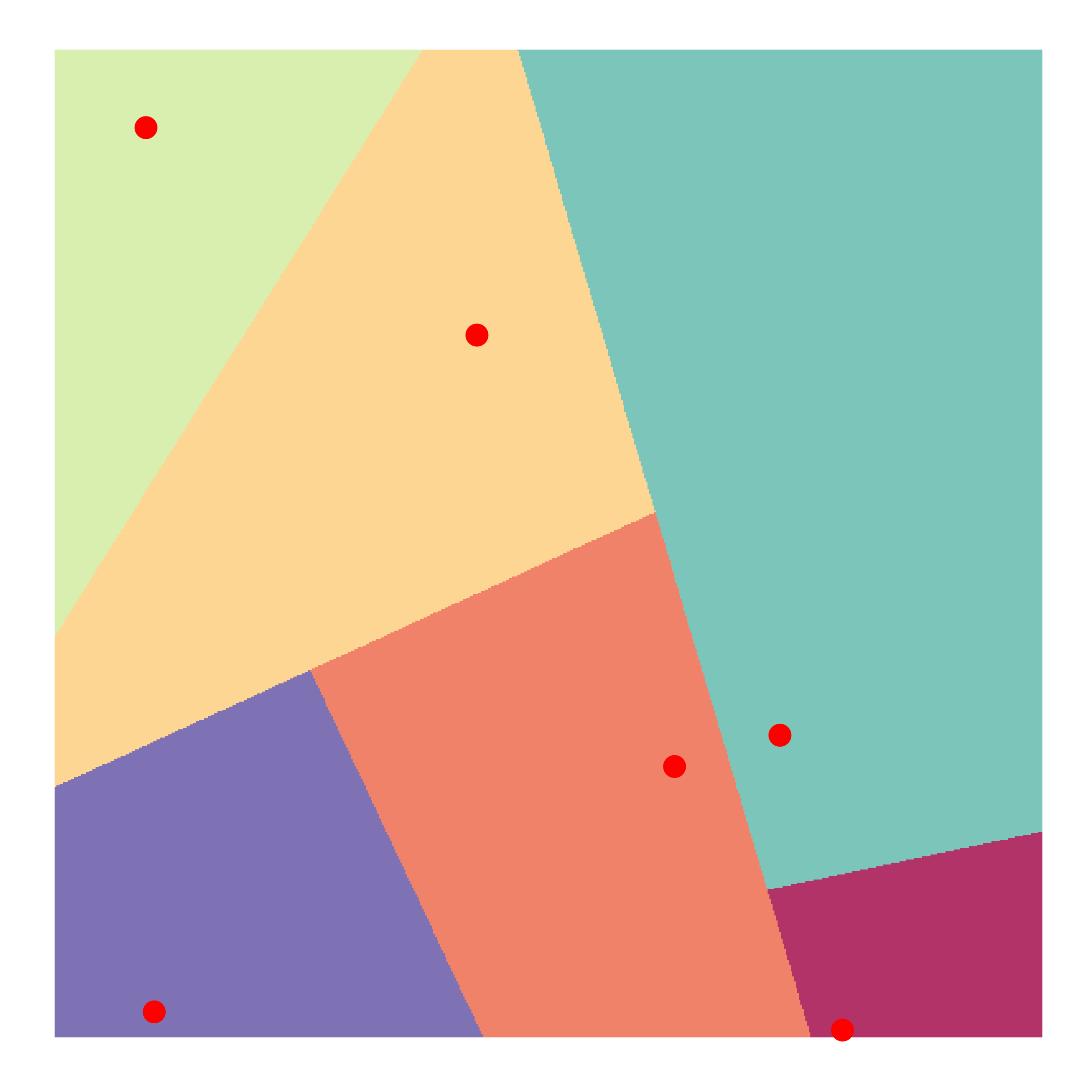
Figure 6: Hierarchical Voronoi representation of “step-surfaces:” in each of the four images, each color corresponds to a single value.

Supplementary material

Appendix E A toy example

Suppose only two measurements are taken from a sensor at times $t_{1}$ and $t_{2}$, to be used as inputs in regression. In our notation, $S_{p}=\{t_{1},t_{2}\}$, $|S_{p}|=p=2$, $X_{S_{p}}=\begin{bmatrix}x_{t_{1}}&x_{t_{2}}\end{bmatrix}$. For simplicity, we call $x_{1}=x_{t_{1}}$, $x_{2}=x_{t_{2}}$, $X_{1}=X_{S_{p}}$, $X_{0}=x_{t_{1}}+x_{t_{2}}$, and we assume its correlation structure depends on parameter $r$ as follows:

$$C(r)=\frac{1}{n}X_{1}^{\prime}X_{1}=\begin{bmatrix}1&r\\ r&1\end{bmatrix}$$

which implies $\frac{1}{n}X_{0}^{\prime}X_{0}=2+2r$. We fix $\beta_{1},\beta_{2},\varepsilon\sim N(0,\sigma^{2}I_{n})$ and set $\bar{\beta}_{1}=\frac{1}{2}(\beta_{1}+\beta_{2})$. We then consider two models

$$\begin{array}[]{ccc}\text{(i)}\quad y=x_{1}\beta_{1}+x_{2}\beta_{2}+\varepsilon&&\text{(ii)}\quad y=(x_{1}+x_{2})\bar{\beta}_{1}+\varepsilon\end{array}$$

Models (i) and (ii) consider the data at the high and low resolutions, respectively. Note that the KL divergence of (ii) from (i) is increasing in $|\beta_{1}-\beta_{2}|$ and decreasing on $r$: high observed correlations (large positive $r$) between covariates make the lower resolution model a good approximation of the high resolution one, and thus we might prefer it, given its increased parsimony.

The KL divergence of the low-res likelihood from the high resolution one is

$$KL(r)=\frac{n}{2\sigma^{2}}(\bar{\beta}-\beta)^{\prime}C(r)(\bar{\beta}-\beta)$$

which is a decreasing function of $r$, since $\frac{\delta}{\delta r}KL(r)=\frac{n}{\sigma^{2}}(\bar{\beta}_{1}-\beta_{1})(\bar{\beta}_{1}-\beta_{2})\leq 0$.

We implement BM&Ms as in Section 3, and get:

$$\begin{array}[]{ccc}\Sigma_{0}=(2(r+1)(n+1))^{-1}&&\Sigma_{1}=\frac{1}{n+1}\begin{bmatrix}1&r\\ r&1\end{bmatrix}^{-1}\\ \mu_{0}=\frac{x_{1}^{\prime}y+x_{2}^{\prime}y}{2(r+1)(n+1)}\xrightarrow[n\to\infty]{}\frac{\beta_{1}+\beta_{2}}{2}&&\mu_{1}=\frac{1}{n+1}\begin{bmatrix}1&r\\ r&1\end{bmatrix}^{-1}\begin{bmatrix}x_{1}^{\prime}e_{1}\\ x_{2}^{\prime}e_{1}\end{bmatrix}\xrightarrow[n\to\infty]{}\begin{bmatrix}\frac{\beta_{1}-\beta_{2}}{2}\\ \frac{\beta_{2}-\beta_{1}}{2}\end{bmatrix}\end{array}$$

Note how $\mu_{0}$ roughly corresponds to the average of the high-resolution coefficient vector, whereas $\mu_{1}$ – which is interpreted as the added detail from the higher resolution – to half differences. Finally, the asymptotic variance of $\theta_{1}=(\theta_{11},\theta_{12})$ becomes

$$AVar(\theta_{1})=\frac{\sigma^{2}}{2(1-r)(r+1)}\begin{bmatrix}3-r&3r-1\\ 3r-1&3-r\end{bmatrix}$$

and this shows that $r\approx 1$ makes the higher resolution worthless. Otherwise, the coefficient vector at the highest resolution can be estimated consistently with BM&Ms via $\mu_{\beta_{M}}$:

$$\mu_{\beta_{M}}=L_{0}\mu_{0}+\mu_{1}=\begin{bmatrix}1&1&0\\ 1&0&1\end{bmatrix}\begin{bmatrix}\mu_{0}\\ \mu_{1}\end{bmatrix}=\begin{bmatrix}\mu_{0}+\mu_{1,1}\\ \mu_{0}+\mu_{1,2}\end{bmatrix}\xrightarrow[n\to\infty]{}\begin{bmatrix}\frac{\beta_{1}+\beta_{2}}{2}\\ \frac{\beta_{1}+\beta_{2}}{2}\end{bmatrix}+\begin{bmatrix}\frac{\beta_{1}-\beta_{2}}{2}\\ \frac{\beta_{2}-\beta_{1}}{2}\end{bmatrix}=\begin{bmatrix}\beta_{1}\\ \beta_{2}\end{bmatrix}$$

We now consider the finite-sample frequentist MSE of

$$\mu^{c}_{\beta_{1,M}} =L_{0}\mu_{0}+c\mu_{1}=L_{0}\mu_{0}+cl\hat{\beta}-c\Sigma_{1}X_{1}^{\prime}X_{0}\mu_{0}=(1-cl)L_{0}\mu_{0}+cl\hat{\beta}$$

with $c\in\{0,1\}$ and $l=\frac{n}{n+1}$. If we select $c=0$, we are estimating $\beta$ through $L_{0}\mu_{0}$, meaning that we completely discard the contribution of the high resolution. The MSE of this estimator for $c=0$ and $c=1$ is, respectively:

$$\text{MSE}(\mu^{c=0}_{\beta_{1,M}}) =((l-2)^{2}+l^{2})\frac{\beta_{1}^{2}+\beta_{2}^{2}}{4}+l(l-2)\beta_{1}\beta_{2}+\frac{\sigma^{2}_{1}}{n(1+r)}$$

$$\text{MSE}(\mu^{c=1}_{\beta_{1,M}}) =(1-l)^{2}((l-2)^{2}+l^{2})\frac{\beta_{1}^{2}+\beta_{2}^{2}}{4}+(1-l)^{2}l(l-2)\beta_{1}\beta_{2}+\frac{2l^{2}\sigma^{2}_{1}}{n(1+r)(1-r)}$$

First, for $n\to\infty$ the bias term approaches $0$ only for $c=1$, whereas the variance will decrease in both cases with $n$. A more relevant scenario is $r\approx 1$ and/or $\beta_{1}\approx\beta_{2}$: if $c=1$ the variance diverges when $r\to 1$. In other words, if $r$ is large, considering the two measurements separately leads to a large expected error. Similarly, $\beta_{1}\approx\beta_{2}$ results in

$$\text{MSE}(\mu^{c=0}_{\beta_{1,M}})_{\beta_{1}\approx\beta_{2}} =2(1-l)^{2}{\beta_{1}^{2}}+\frac{\sigma^{2}_{1}}{n(1+r)}$$

$$\text{MSE}(\mu^{c=1}_{\beta_{1,M}})_{\beta_{1}\approx\beta_{2}} =2(1-l)^{4}{\beta_{1}^{2}}+\frac{2l^{2}\sigma^{2}_{1}}{n(1+r)(1-r)}$$

meaning that the bias term is almost equalized, but favoring $c=0$, whereas the comparison on variance entirely depends on $r$: the closer the two coefficients $\beta_{1}$ and $\beta_{2}$ are to each other, the closer to zero $r$ must be to make it worth it to consider the high resolution. Ultimately, this shows how considering the data at the highest resolution might be counterproductive. An alternative way to visualize why $c=1$ may be suboptimal is to look at $\mu^{c}_{\beta_{1,M}}$ (with $c\in[0,1]$ ) as an estimator that shrinks towards the lower resolution coefficient function.

E.1 Modules for BM&Ms in example

Module 0:

$$y=\theta_{0}(x_{1}+x_{2})+\varepsilon_{0}\quad\text{where}\quad\varepsilon_{0}\sim N(0,\sigma^{2}_{0}I_{n})$$

with prior parameters $m_{0}=0$ and $M_{0}=n((x_{1}+x_{2})^{\prime}(x_{1}+x_{2}))^{-1}=\frac{1}{2}(r+1)^{-1}$. We get

$$\Sigma_{0} =(2(r+1)+2n(r+1))^{-1}=(2(r+1)(n+1))^{-1}$$

$$\mu_{0} =\frac{(x_{1}+x_{2})^{\prime}y}{2(r+1)(n+1)}=\frac{n\frac{x_{1}^{\prime}y}{n}+n\frac{x_{2}^{\prime}y}{n}}{2(r+1)(n+1)}\xrightarrow[n\to\infty]{}\frac{\beta_{1}+\beta_{2}}{2}$$

Module 1:

$$e_{1}=\begin{bmatrix}x_{1}&x_{2}\end{bmatrix}\begin{bmatrix}\theta_{11}\\ \theta_{12}\end{bmatrix}+\varepsilon_{1}\quad\text{where}\quad\varepsilon_{1}\sim N(0,\sigma^{2}_{1})$$

where $e_{1}=y-(x_{1}+x_{2})\frac{(x_{1}+x_{2})^{\prime}y}{2(r+1)(n+1)}$. In this case we set the prior parameters as

$$\begin{array}[]{ccc}m_{1}=\begin{bmatrix}m_{11}&m_{12}\end{bmatrix}=\begin{bmatrix}0&0\end{bmatrix}&&M_{1}=n\begin{bmatrix}1&r\\ r&1\end{bmatrix}^{-1},\end{array}$$

hence the posterior parameters are

$$\Sigma_{1} =\frac{1}{n+1}\begin{bmatrix}1&r\\ r&1\end{bmatrix}^{-1}$$

$$\mu_{1} =\frac{1}{n+1}\begin{bmatrix}1&r\\ r&1\end{bmatrix}^{-1}\begin{bmatrix}x_{1}^{\prime}e_{1}\\ x_{2}^{\prime}e_{1}\end{bmatrix}$$

$$=\frac{1}{n+1}\begin{bmatrix}1&r\\ r&1\end{bmatrix}^{-1}\begin{bmatrix}x_{1}^{\prime}y-x_{1}^{\prime}(x_{1}+x_{2})\frac{(x_{1}+x_{2})^{\prime}y}{2(r+1)(n+1)}\\ x_{2}^{\prime}y-x_{2}^{\prime}(x_{1}+x_{2})\frac{(x_{1}+x_{2})^{\prime}y}{2(r+1)(n+1)}\end{bmatrix}$$

$$\xrightarrow[n\to\infty]{}\begin{bmatrix}1&r\\ r&1\end{bmatrix}^{-1}\begin{bmatrix}\beta_{1}+r\beta_{2}-(r+1)\frac{\beta_{1}+\beta_{2}}{2}\\ r\beta_{1}+\beta_{2}-(r+1)\frac{\beta_{1}+\beta_{2}}{2}\end{bmatrix}$$

$$=\frac{1}{r+1}\begin{bmatrix}1&-r\\ -r&1\\ \end{bmatrix}\begin{bmatrix}\frac{1}{2}\beta_{1}-\frac{1}{2}\beta_{2}\\ \frac{1}{2}\beta_{2}-\frac{1}{2}\beta_{1}\end{bmatrix}\frac{1}{r+1}\begin{bmatrix}1&-r\\ -r&1\\ \end{bmatrix}(\beta-L_{0}C_{0}\beta)=\begin{bmatrix}\frac{\beta_{1}-\beta_{2}}{2}\\ \frac{\beta_{2}-\beta_{1}}{2}\end{bmatrix},$$

where $C_{0}=\begin{bmatrix}\frac{1}{2}&\frac{1}{2}\end{bmatrix}$. $\Sigma_{1}$ is the posterior covariance of $\theta_{1}|\theta_{0}$, whereas the asymptotic variance of $\theta_{1}=(\theta_{11},\theta_{12})$ is

$$AVar(\theta_{1}) =\Omega_{1}^{-1}+\sigma^{2}L_{0}\Omega_{0}^{-1}L_{0}^{\prime}$$

$$=\sigma^{2}\left(\begin{bmatrix}1&r\\ r&1\end{bmatrix}^{-1}+\frac{1}{2(r+1)}L_{0}L_{0}^{\prime}\right)$$

$$=\sigma^{2}\left(\frac{1}{(1-r)(r+1)}\begin{bmatrix}1&-r\\ -r&1\end{bmatrix}+\frac{1}{2(r+1)}\begin{bmatrix}1&1\\ 1&1\end{bmatrix}\right)$$

$$=\frac{\sigma^{2}}{r+1}\left(\frac{1}{1-r}\begin{bmatrix}1&-r\\ -r&1\end{bmatrix}+\frac{1}{2}\begin{bmatrix}1&1\\ 1&1\end{bmatrix}\right)=\frac{\sigma^{2}}{r+1}\left(\begin{bmatrix}\frac{1}{1-r}&\frac{-r}{1-r}\\ \frac{-r}{1-r}&\frac{1}{1-r}\end{bmatrix}+\begin{bmatrix}\frac{1}{2}&\frac{1}{2}\\ \frac{1}{2}&\frac{1}{2}\end{bmatrix}\right)$$

$$=\frac{\sigma^{2}}{r+1}\begin{bmatrix}\frac{2+1-r}{2(1-r)}&\frac{-2r+1-r}{2(1-r)}\\ \frac{-2r+1-r}{2(1-r)}&\frac{2+1-r}{2(1-r)}\end{bmatrix}=\frac{\sigma^{2}}{r+1}\begin{bmatrix}\frac{3-r}{2(1-r)}&\frac{1-3r}{2(1-r)}\\ \frac{1-3r}{2(1-r)}&\frac{3-r}{2(1-r)}\end{bmatrix}$$

$$=\frac{\sigma^{2}}{2(1-r)(r+1)}\begin{bmatrix}3-r&3r-1\\ 3r-1&3-r\end{bmatrix}$$

E.2 MSE for $\mu^{c}_{\beta_{1},M}$

The expected value of the modular estimator for $\beta$ is

$$E\left[\mu^{c}_{\beta_{1,M}}\right] =E\left[(1-cl)L_{0}\mu_{0}+cl\hat{\beta}\right]$$

$$=E\left[l(1-cl)L_{0}(X_{0}^{\prime}X_{0})^{-1}X_{0}^{\prime}y+cl\hat{\beta}\right]$$

$$=E\left[l(1-cl)L_{0}(X_{0}^{\prime}X_{0})^{-1}X_{0}^{\prime}(X_{1}\beta+\varepsilon_{1})\right]+cl\beta$$

$$=l(1-cl)L_{0}(X_{0}^{\prime}X_{0})^{-1}X_{0}^{\prime}X_{1}\beta+cl\beta$$

$$=(l(1-cl)L_{0}(X_{0}^{\prime}X_{0})^{-1}X_{0}^{\prime}X_{1}+cl)\beta$$

$$=(l(1-cl)\begin{bmatrix}\frac{1}{2n(r+1)}\\ \frac{1}{2n(r+1)}\end{bmatrix}\begin{bmatrix}n(1+r)&n(1+r)\end{bmatrix}+cl)\beta$$

$$=l(1-cl)\begin{bmatrix}\frac{\beta_{1}+\beta_{2}}{2}\\ \frac{\beta_{1}+\beta_{2}}{2}\end{bmatrix}+cl\begin{bmatrix}\beta_{1}\\ \beta_{2}\end{bmatrix}$$

so that the estimator has bias

$$E\left[\mu^{c}_{\beta_{1,M}}\right]-\beta =\frac{1-cl}{2}\begin{bmatrix}l-2&l\\ l&l-2\end{bmatrix}\beta$$

which, as expected, is smaller for $l\approx 1$. We also obtain

$$\text{Bias}^{2} =\frac{(1-cl)^{2}}{4}\beta^{\prime}\begin{bmatrix}(l-2)^{2}+l^{2}&2(l-2)l\\ 2(l-2)l&(l-2)^{2}+l^{2}\end{bmatrix}\beta$$

$$=(1-cl)^{2}((l-2)^{2}+l^{2})\frac{\beta_{1}^{2}+\beta_{2}^{2}}{4}+(1-cl)^{2}l(l-2)\beta_{1}\beta_{2}$$

We then move to calculating the variance of $\mu_{\beta}$.

$$Var(\mu^{c}_{\beta_{1,M}}) =Var((1-cl)L_{0}(X_{0}^{\prime}X_{0})^{-1}X_{0}^{\prime}y+cl(X_{1}^{\prime}X_{1})^{-1}X_{1}^{\prime}y)$$

$$=Var(((1-cl)L_{0}(X_{0}^{\prime}X_{0})^{-1}X_{0}^{\prime}+cl(X_{1}^{\prime}X_{1})^{-1}X_{1}^{\prime})\varepsilon)$$

$$=\sigma^{2}_{1}((1-cl)L_{0}(X_{0}^{\prime}X_{0})^{-1}X_{0}^{\prime}+cl(X_{1}^{\prime}X_{1})^{-1}X_{1}^{\prime})((1-cl)L_{0}(X_{0}^{\prime}X_{0})^{-1}X_{0}^{\prime}+cl(X_{1}^{\prime}X_{1})^{-1}X_{1}^{\prime})^{\prime}$$

$$=\sigma^{2}_{1}((1-cl)^{2}L_{0}(X_{0}^{\prime}X_{0})^{-1}L_{0}^{\prime}+cl(1-cl)L_{0}(X_{0}^{\prime}X_{0})^{-1}X_{0}^{\prime}X_{1}(X_{1}^{\prime}X_{1})^{-1}$$

$$\qquad+cl(1-cl)(X_{1}^{\prime}X_{1})^{-1}X_{1}^{\prime}X_{0}(X_{0}^{\prime}X_{0})^{-1}L_{0}^{\prime}+c^{2}l^{2}(X_{1}^{\prime}X_{1})^{-1})$$

$$=\sigma^{2}_{1}\left(\frac{(1-cl)^{2}}{2n(r+1)}\begin{bmatrix}1&1\\ 1&1\end{bmatrix}+\frac{cl(1-cl)}{2n(r+1)(1-r^{2})}\begin{bmatrix}1\\ 1\end{bmatrix}\begin{bmatrix}1+r&1+r\end{bmatrix}\begin{bmatrix}1&-r\\ -r&1\end{bmatrix}+\right.$$

$$\qquad+\left.\frac{cl(1-cl)}{n(1-r^{2})(r+1)}\begin{bmatrix}1&-r\\ -r&1\end{bmatrix}\begin{bmatrix}1+r\\ 1+r\end{bmatrix}\begin{bmatrix}1&1\end{bmatrix}+\frac{c^{2}l^{2}}{n(1-r^{2})}\begin{bmatrix}1&-r\\ -r&1\end{bmatrix}\right)$$

$$=\sigma^{2}_{1}\left(\frac{(1-cl)^{2}}{2n(r+1)}\begin{bmatrix}1&1\\ 1&1\end{bmatrix}+\frac{cl(1-cl)}{2n(1-r)(1+r)}\begin{bmatrix}1-r&1-r\\ 1-r&1-r\end{bmatrix}+\right.$$

$$\left.\qquad+\frac{cl(1-cl)}{2n(1+r)}\begin{bmatrix}1&1\\ 1&1\end{bmatrix}+\frac{c^{2}l^{2}}{n(1-r^{2})}\begin{bmatrix}1&-r\\ -r&1\end{bmatrix}\right)$$

$$=\frac{\sigma^{2}_{1}}{n(1+r)}\left(\frac{(1-cl)^{2}}{2}\begin{bmatrix}1&1\\ 1&1\end{bmatrix}+cl(1-cl)\begin{bmatrix}1&1\\ 1&1\end{bmatrix}+\frac{c^{2}l^{2}}{1-r}\begin{bmatrix}1&-r\\ -r&1\end{bmatrix}\right)$$

And then finally

$$\text{Tr}(\text{Var}(\mu^{c}_{\beta_{1,M}})) =\frac{\sigma^{2}_{1}}{n(1+r)}\left((1-cl)(1+cl)+\frac{2c^{2}l^{2}}{1-r}\right)$$

So that the modular estimator has mean square error:

$$\text{MSE}(\mu^{c}_{\beta_{1,M}}) =(1-cl)^{2}((l-2)^{2}+l^{2})\frac{\beta_{1}^{2}+\beta_{2}^{2}}{4}+(1-cl)^{2}l(l-2)\beta_{1}\beta_{2}+$$

$$\qquad+\frac{\sigma^{2}_{1}}{n(1+r)}\left((1-cl)(1+cl)+\frac{2c^{2}l^{2}}{1-r}\right)$$

References

- Albert and Chib, (1993) Albert, J. H. and Chib, S. (1993). Bayesian analysis of binary and polychotomous response data. Journal of the American Statistical Association, 88(422):669–679.
- Brown et al., (2001) Brown, P. J., Fearn, T., and Vannucci, M. (2001). Bayesian wavelet regression on curves with application to a spectroscopic calibration problem. Journal of the American Statistical Association, 96(454):398–408.
- Bühlmann and van de Geer, (2011) Bühlmann, P. and van de Geer, S. (2011). Statistics for High-Dimensional Data. Springer, Dordrecht.
- Chen and Dunson, (2017) Chen, Y. and Dunson, D. B. (2017). Modular bayes screening for high-dimensional predictors. arXiv:1703.09906.
- Delaigle and Hall, (2012) Delaigle, A. and Hall, P. (2012). Methodology and theory for partial least squares applied to functional data. The Annals of Statistics, 40(1):322–352.
- Donoho and Johnstone, (1994) Donoho, D. L. and Johnstone, I. M. (1994). Ideal spatial adaptation by wavelet shrinkage. Biometrika, 81:425–455.
- Donoho and Johnstone, (1995) Donoho, D. L. and Johnstone, I. M. (1995). Adapting to unknown smoothness via wavelet shrinkage. Journal of the American Statistical Association, 90:1200–1224.
- Essen et al., (2013) Essen, D. C. V., Smith, S. M., Barch, D. M., Behrens, T. E., Yacoub, E., and Kamil Ugurbil, f. t. W.-M. H. C. (2013). The wu-minn human connectome project: An overview. NeuroImage, 80(2013):62–79.
- Garrett and Hough, (2018) Garrett, B. and Hough, G. (2018). Brain & Behavior: an introduction to Behavioral Neuroscience. SAGE Publications, 5th edition.
- Gelman et al., (2014) Gelman, A., Carlin, J., Stern, H., Dunson, D., Vehtari, A., and Rubin, D. (2014). Bayesian Data Analysis, Third Edition (Chapman & Hall/CRC Texts in Statistical Science). Chapman and Hall/CRC, third edition.
- Geweke, (2005) Geweke, J. (2005). Contemporary Bayesian econometrics and statistics. Wiley-Interscience.
- Glasser et al., (2013) Glasser, M. F., Sotiropoulos, S. N., Wilson, J. A., Coalson, T. S., Fischl, B., Andersson, J. L., Xu, J., Jbabdi, S., Webster, M., Polimeni, J. R., Essen, D. C. V., and Jenkinson, M. (2013). The minimal preprocessing pipelines for the human connectome project. NeuroImage, 80(2013):105–124.
- Gong et al., (2011) Gong, G., He, Y., and Evans, A. C. (2011). Brain connectivity: gender makes a difference. The Neuroscientist, 17:575–591.
- Gordon et al., (2016) Gordon, E. M., Laumann, T. O., Adeyemo, B., Huckins, J. F., Kelley, W. M., and Petersen, S. E. (2016). Generation and evaluation of a cortical area parcellation from resting-state correlations. Cerebral Cortex, 26(1):288–303.
- Green, (1995) Green, P. J. (1995). Reversible jump markov chain monte carlo computation and Bayesian model determination. Biometrika, 82(4):711–732.
- Guhaniyogi et al., (2017) Guhaniyogi, R., Qamar, S., and Dunson, D. B. (2017). Bayesian tensor regression. Journal of Machine Learning Research, 18(79):1–31.
- Hoerl, (1962) Hoerl, A. E. (1962). Application of ridge analysis to regression problems. Chemical Engineering Progress, 58:54–59.
- Jacob et al., (2017) Jacob, P. E., Murray, L. M., Holmes, C. C., and Robert, C. P. (2017). Better together? statistical learning in models made of modules. arXiv:1708.08719.
- Jeong et al., (2013) Jeong, J., Vannucci, M., and Ko, K. (2013). A wavelet-based Bayesian approach to regression models with long memory errors and its application to fMRI data. Biometrics, 69:184–196.
- Kaisera et al., (2009) Kaisera, A., Hallerb, S., Schmitzd, S., and Nitscha, C. (2009). On sex/gender related similarities and differences in fMRI language research. Brain Research Reviews, 61:49–59.
- Kleijn and van der Vaart, (2012) Kleijn, B. and van der Vaart, A. (2012). The bernstein-von-mises theorem under misspecification. Electron. J. Statist., 6:354–381.
- Lee et al., (2014) Lee, M. R., Cacic, K., Demers, C. H., Haroon, M., Heishman, S., Hommer, D. W., Epstein, D. H., J.Ross, T., Stein, E. A., Heilig, M., and Salmeron, B. J. (2014). Gender differences in neural–behavioral response to self-observation during a novel fMRI social stress task. Neuropsychologia, 53:257–263.
- Li and Zhang, (2010) Li, F. and Zhang, N. R. (2010). Bayesian variable selection in structured high-dimensional covariate spaces with applications in genomics. Journal of the American Statistical Association, 105(491):1202–1214, https://doi.org/10.1198/jasa.2010.tm08177.
- Li et al., (2018) Li, X., Xu, D., Zhou, H., and Li, L. (2018). Tucker tensor regression and neuroimaging analysis. Statistics in Biosciences.
- Liu et al., (2009) Liu, F., Bayarri, M. J., and Berger, J. O. (2009). Modularization in Bayesian analysis, with emphasis on analysis of computer models. Bayesian Analysis, 4(1):119–150.
- Marin and Robert, (2007) Marin, J.-M. and Robert, C. P. (2007). Bayesian core: a practical approach to computational Bayesian statistics. Springer Publishing Company, Incorporated.
- Morris, (2015) Morris, J. S. (2015). Functional regression. Annual Review of Statistics and Its Application, 2(1):321–359.
- Murphy and Topel, (1985) Murphy, K. M. and Topel, R. H. (1985). Estimation and inference in two-step econometric models. Journal of Business & Economic Statistics, 3(4):370–379.
- Nason, (2008) Nason, G. (2008). Wavelet Methods in Statistics with R. Springer Publishing Company, Incorporated, 1st edition.
- Nason and Silverman, (1994) Nason, G. P. and Silverman, B. W. (1994). The discrete wavelet transform in s. Journal of Computational and Graphical Statistics, 3(2):163–191.
- Plummer, (2015) Plummer, M. (2015). Cuts in Bayesian graphical models. Statistics and Computing, 25(1):37–43.
- Ramsay and Silverman, (1997) Ramsay, J. and Silverman, B. (1997). Functional Data Analysis. Springer Publishing Company, Incorporated.
- Reiss et al., (2017) Reiss, P. T., Goldsmith, J., Shang, H. L., and Ogden, R. T. (2017). Methods for scalar-on-function regression. International Statistical Review, 85(2):228–249.
- Scarlett and Cevher, (2017) Scarlett, J. and Cevher, V. (2017). Limits on support recovery with probabilistic models: An information-theoretic framework. IEEE Transaction on Information Theory, 63:593 – 620.
- Schiffler et al., (2017) Schiffler, P., Tenberge, J.-G., Wiendl, H., and Meuth, S. G. (2017). Cortex parcellation associated whole white matter parcellation in individual subjects. Frontiers in Human Neuroscience, 11:352.
- Thirion et al., (2014) Thirion, B., Varoquaux, G., Dohmatob, E., and Poline, J.-B. (2014). Which fMRI clustering gives good brain parcellations? Frontiers in Neuroscience, 8:167.
- Tibshirani, (1996) Tibshirani, R. (1996). Regression shrinkage and selection via the lasso. Journal of the Royal Statistical Society: Series B, 58:267–288.
- Tibshirani et al., (2005) Tibshirani, R., Saunders, M., Rosset, S., Zhu, J., and Knight, K. (2005). Sparsity and smoothness via the fused lasso. Journal of the Royal Statistical Society: Series B, pages 91–108.
- Tomasi and Volkow, (2012) Tomasi, D. and Volkow, N. D. (2012). Gender differences in brain functional connectivity density. Human Brain Mapping, 33:849–860.
- Wasserman and Roeder, (2009) Wasserman, L. and Roeder, K. (2009). High dimensional variable selection. Annals of Statistics, 37(5A):2178–2201.
- Yuan and Lin, (2006) Yuan, M. and Lin, Y. (2006). Model selection and estimation in regression with grouped variables. Journal of the Royal Statistical Society, Series B, 68:49–67.
- Zhao and Yu, (2006) Zhao, P. and Yu, B. (2006). On model selection consistency of lasso. Journal of Machine Learning Research, 7:2541–2563.
- Zhao et al., (2012) Zhao, Y., Ogden, R. T., and Reiss, P. T. (2012). Wavelet-based lasso in functional linear regression. Journal of Computational and Graphical Statistics, 21(3):600–617.
- Zhou et al., (2013) Zhou, H., Li, L., and Zhu, H. (2013). Tensor regression with applications in neuroimaging data analysis. Journal of the American Statistical Association, 108(502):540–552.