Breast Cancer Detection through Electrical Impedance Tomography and Optimal Control Theory: Theoretical and Computational Analysis

Abstract.

The Inverse Electrical Impedance Tomography (EIT) problem on recovering electrical conductivity tensor and potential in the body based on the measurement of the boundary voltages on the electrodes for a given electrode current is analyzed. A PDE constrained optimal control framework in Besov space is pursued, where the electrical conductivity tensor and boundary voltages are control parameters, and the cost functional is the norm declinations of the boundary electrode current from the given current pattern and boundary electrode voltages from the measurements. The state vector is a solution of the second order elliptic PDE in divergence form with bounded measurable coefficients under mixed Neumann/Robin type boundary condition. Existence of the optimal control and Fréchet differentiability in the Besov space setting is proved. The formula for the Fréchet gradient and optimality condition is derived. Extensive numerical analysis is pursued in the 2D case by implementing the projective gradient method, re-parameterization via principal component analysis (PCA) and Tikhonov regularization. Breast cancer detection, Electrical Impedance Tomography, PDE constrained optimal control, Fréchet differentiability, projective gradient method, principal component analysis, Tikhonov regularization.

1. Introduction and Problem Description

This paper analyzes mathematical model for the breast cancer detection through EIT. Let $Q\in\mathbb{R}^{n}$ be an open and bounded set representing body, and assume $A(x)=\big{(}a_{ij}(x)\big{)}_{ij=1}^{n}$ be a matrix representing the electrical conductivity tensor at the point $x\in Q$. Electrodes, $(E_{l})_{l=1}^{m}$, with contact impedances vector $Z:=(Z_{l})_{l=1}^{m}\in\mathbb{R}^{m}_{+}$ are attached to the periphery of the body, $\partial Q$. Electrical currents vector $I:=(I_{l})_{l=1}^{m}\in\mathbb{R}^{m}$ is applied to the electrodes. Vector $I$ is called current pattern if it satisfies conservation of charge condition

(1.1) $$\sum_{l=1}^{m}I_{l}=0$$

The induced constant voltage on electrodes is denoted by $U:=(U_{l})_{l=1}^{m}\in\mathbb{R}^{m}$. By specifying ground or zero potential it is assumed that

(1.2) $$\sum_{l=1}^{m}U_{l}=0$$

EIT problem is to find the electrostatic potential $u:Q\to\mathbb{R}$ and boundary voltages $U$ on $(E_{l})_{l=1}^{m}$. The mathematical model of the EIT problem is described through the following boundary value problem for the second order elliptic partial differential equation:

(1.3) $$-\sum_{i,j=1}^{n}\big{(}a_{ij}(x)u_{x_{j}}\big{)}_{x_{i}}=0, \quad x\in Q$$

(1.4) $$\frac{\partial u(x)}{\partial\mathcal{N}}=0, \quad x\in\partial Q-\bigcup\limits_{l=1}^{m}E_{l}$$

(1.5) $$u(x)+Z_{l}\frac{\partial u(x)}{\partial\mathcal{N}}=U_{l}, \quad x\in E_{l},\ l=\overline{1,m}$$

(1.6) $$\displaystyle\int_{E_{l}}\frac{\partial u(x)}{\partial\mathcal{N}}ds=I_{l}, \quad l=\overline{1,m}$$

where

$$\frac{\partial u(x)}{\partial\mathcal{N}}=\sum_{i,j}a_{ij}(x)u_{x_{j}}\nu^{i}$$

be a co-normal derivative at $x$, and $\nu=(\nu^{1},...,\nu^{n})$ is the outward normal at a point $x$ to $\partial Q$. Electrical conductivity matrix $A=(a_{ij})$ is positive definite with

(1.7) $$\sum_{i,j=1}^{n}a_{ij}(x)\xi_{i}\xi_{j}\geq\mu\displaystyle\sum_{i=1}^{n}\xi_{i}^{2},\ \forall\xi\in\mathbb{R}^{n};\quad\mu>0.$$

The following is the

EIT Problem: Given electrical conductivity tensor $A$, electrode contact impedance vector $Z$, and electrode current pattern $I$ it is required to find electrostatic potential $u$ and electrode voltages $U$ satisfying (1.2)–(1.6):

$$(A,Z,I)\longrightarrow(u,U)$$

The goal of the paper is to analyze inverse EIT problem of determining conductivity tensor $A$ from the measurements of the boundary voltages $U^{*}$.

Inverse EIT Problem: Given electrode contact impedance vector $Z$, electrode current pattern $I$ and boundary electrode measurement $U^{*}$, it is required to find electrostatic potential $u$ and electrical conductivity tensor $A$ satisfying (1.2)–(1.6) with $U=U^{*}$.

Mathematical model (1.2)–(1.6) for the EIT Problem was suggested in Cheng et al. (1989). In Somersalo et al. (1992) it was demonstrated that the model is capable of predicting the experimentally measured voltages to within 0.1 percent. Existence and uniqueness of the solution to the problem (1.2)-(1.6) was also proved in Somersalo et al. (1992). EIT is a rapidly developing non-invasive imaging technique recently gaining popularity in various medical applications including breast screening and cancer detection Zou & Guo (2003); Brown (2003); Adler et al. (n.d.); Holder (2004). The objective of the Inverse EIT Problem is reconstructing the electrical conductivity through measuring voltages of electrodes placed on the surface of a test volume. The electrical conductivity of the malignant tumors of the breast may significantly differ from the conductivity of surrounding normal tissue. This provides a possible way to develop an efficient, safe and inexpensive method to detect and localize such tumors. X-ray mammography, ultrasound, and magnetic resonance imaging (MRI) are among methods that are used currently for breast cancer diagnosis Zou & Guo (2003). However, these methods have various flaws and cannot distinguish breast cancer from benign breast lesions with certainty Zou & Guo (2003). EIT is a fast, inexpensive, portable, and relatively harmless technique, although it also has the disadvantage of poor image resolution Paulson et al. (1995). Different types of regularization have been applied to overcome this issue Brown (2003); Adler & Lionheart (2005). Inverse EIT Problem is an ill-posed problem and belongs to the class of so-called Calderon type inverse problems, due to pioneering work Calderon (1980) where well-posedness of the inverse problem for the identification of the conductivity coefficient of the second order elliptic PDE through Dirichlet-to-Neumann or Neumann-to-Dirichlet maps is presented. We refer to topical review paper Borcea (2002) on EIT and Calderon type inverse problems. Reconstruction of the coefficient in Calderon problem is pursued in Nachman (1988),and the uniqueness of the solution has been demonstrated Sylvester & Uhlmann (1987). This framework was shown to be stable in Alessandrini (1988). Well-posedness of the inverse Calderon problem with partial boundary data is analyzed in Kenig et al. (2007). Statistical methods have been applied for solving inverse EIT problem in Kaipio et al. (2000, 1999); Roininen et al. (2014). Bayesian formulation of EIT in infinite dimensions has been proposed in Dunlop & Stuart (2016). An experimental iterative algorithm, POMPUS, was introduced, the accuracy of which is comparable to standard Newton-based algorithms Paulson et al. (1995). An analytic solution for potential distribution on a 2D homogeneous disk for EIT problem was analyzed in Demidenko (2011). A statistical model called gapZ, has also been developed for solving EIT using Toeplitz matrices Demidenko et al. (2011).

In this paper, inverse EIT Problem is investigated with unknown electrical conductivity tensor $A$. This is in contrast with current state of the art in the field where usually inverse EIT problem is solved for the reconstruction of the single conductivity function. This novelty is essential in understanding and detection of the highly anisotropic distribution of the cancerous tumor in breast. We formulate Inverse EIT Problem as a PDE constrained optimal control problem in Besov spaces framework, where the electrical conductivity tensor and boundary voltages are control parameters, and the cost functional is the norm declinations of the boundary electrode current from the given current pattern and boundary electrode voltages from the measurements. We prove the existence of the optimal control and Fréchet differentiability in the Besov space setting. The formula for the Fréchet gradient and optimality condition is derived. Based on the Fréchet differentiability result we develop projective gradient method in Besov spaces. Extensive numerical analysis in the 2D case by implementing the projective gradient method, re-parameterization via PCA and Tikhonov regularization is pursued.

The organization of the paper is as follows. In Section 2 we introduce the notations of the functional spaces. In Section 3 we introduce Inverse EIT Problem as PDE constrained optimal control problem. In Section 4 we formulate the main results. Proof of the main results are presented in Section 5. In Section 6 we present the results of the computational analysis for the 2D model. Finally, in Section 7 we outline the main conclusions.

2. Notations

In this section, assume $Q$ is a domain in $\mathbb{R}^{n}$.

• For $1\leq p<\infty$, $L_{p}(Q)$ is a Banach space of measurable functions on $Q$ with finite norm

  $$\|u\|_{L_{p}(Q)}:=\Big{(}\int_{Q}|u(x)|^{p}dx\Big{)}^{\frac{1}{p}}$$

  In particular if $p=2$, $L_{2}(Q)$ is a Hilbert space with inner product

  $$(f,g)_{L_{2}(Q)}=\int_{Q}f(x)g(x)dx$$

• $L_{\infty}(Q)$ is a Banach space of measurable functions on $Q$ with finite norm

  $$\|u\|_{L_{\infty}(Q)}:=\text{ess}\displaystyle\sup_{x\in Q}|u(x)|$$

• For $s\in\mathbb{Z}_{+}$, $W_{p}^{s}(Q)$ is the Banach space of measurable functions on $Q$ with finite norm

  $$\|u\|_{W_{p}^{s}(Q)}:=\Big{(}\int_{Q}\displaystyle\sum_{|\alpha|\leq s}|D^{\alpha}u(x)|^{p}dx\Big{)}^{\frac{1}{p}},$$

  where $\alpha=(\alpha_{1},\alpha_{2},...,\alpha_{n})$, $\alpha_{j}$ are nonnegative integers, $|\alpha|=\alpha_{1}+...+\alpha_{n}$, $D_{k}=\frac{\partial}{\partial x_{k}}$, $D^{\alpha}=D_{1}^{\alpha_{1}}...D_{n}^{\alpha_{n}}.$ In particular if $p=2$, $H^{s}(Q):=W_{2}^{s}(Q)$ is a Hilbert space with inner product

  $$(f,g)_{H^{s}(Q)}=\displaystyle\sum_{|\alpha|\leq s}(D^{\alpha}f(x),D^{\alpha}g(x))_{L_{2}(Q)}$$

• For $s\notin\mathbb{Z}_{+}$, $B_{p}^{s}(Q)$ is the Banach space of measurable functions on $Q$ with finite norm

  $$\|u\|_{B_{p}^{s}(Q)}:=\|u\|_{W_{p}^{[s]}(Q)}+[u]_{B_{p}^{s}(Q)}$$

  where

  $$[u]_{B_{p}^{s}(Q)}:=\int_{Q}\int_{Q}\frac{\big{|}\frac{\partial^{[s]}u(x)}{\partial x^{[s]}}-\frac{\partial^{[s]}u(y)}{\partial x^{[s]}}\big{|}^{p}}{|x-y|^{1+p(s-[s])}}dxdy\Big{)}^{\frac{1}{p}}$$

  $H^{\epsilon}(Q):=B_{2}^{\epsilon}(Q)$ is an Hilbert space.

• $\textbf{ba}(Q)=\big{(}L_{\infty}(Q)\big{)}^{\prime}$ is the Banach space of bounded and finitely additive signed measures on $Q$ and the dual space of $L_{\infty}(Q)$ with finite norm

  $$\|\phi\|_{\textbf{ba}(Q)}=|\phi|(Q),$$

  $|\phi|(Q)$ is total variation of $\phi$ and defined as $|\phi|(Q)=\sup\displaystyle\sum_{i}\phi(E_{i})$, where the supremum is taken over all partitions $\cup E_{i}$ of $E$ into measurable subsets $E_{i}$.

• $\mathbb{M}^{m\times n}$ is a space of real $m\times n$ matrices.

• $\mathscr{L}:=L_{\infty}(Q;\mathbb{M}^{n\times n})$ is the Banach space of $n\times n$ matrices of $L_{\infty}(Q)$ functions.

• $\mathscr{L}^{\prime}:=\textbf{ba}(Q;\mathbb{M}^{n\times n})=\bigl{(}L_{\infty}(Q;\mathbb{M}^{n\times n})\bigr{)}^{\prime}$ is the Banach space of $n\times n$ matrices of $\textbf{ba}(Q)$ measures.

3. Optimal Control Problem

We formulate Inverse EIT Problem as the following PDE constrained optimal control problem. Consider the minimization of the cost functional

(3.1) $$\mathcal{J}(v)=\displaystyle\sum_{l=1}^{m}\Big{|}\displaystyle\int_{E_{l}}\frac{U_{l}-u(x)}{Z_{l}}ds-I_{l}\Big{|}^{2}+\beta|U-U^{*}|^{2}$$

on the control set

$$V_{R}=\big{\{}v=(A,U)\in\Big{(}L_{\infty}(Q;\mathbb{M}^{n\times n})\bigcap H^{\epsilon}(Q;\mathbb{M}^{n\times n})\Big{)}\times\mathbb{R}^{m}\Big{|}\sum_{l=1}^{m}U_{l}=0,$$

$$\|A\|_{L_{\infty}}+\|A\|_{H^{\epsilon}}+|U|\leq R,\ \xi^{T}A\xi\geq\mu|\xi|^{2},\ \forall\xi\in\mathbb{R}^{n},\ \mu>0\big{\}}$$

where $\beta>0$, and $u=u(\cdot;v)\in H^{1}(Q)$ is a solution of the elliptic problem (1.3)–(1.5). This optimal control problem will be called Problem $\mathcal{J}$. The first term in the cost functional $\mathcal{J}(v)$ characterizes the mismatch of the condition (1.6) in light of the Robin condition (1.5).

Note that the variational formulation of the EIT Problem is a particular case of the Problem $\mathcal{J}$, when the conductivity tensor $A$ is known, and therefore is removed from the control set by setting $R=+\infty$ and $\beta=0$:

(3.2) $$\mathcal{I}(U)=\displaystyle\sum_{l=1}^{m}\Big{|}\displaystyle\int_{E_{l}}\frac{U_{l}-u(x)}{Z_{l}}ds-I_{l}\Big{|}^{2}\to\inf$$

in a control set

(3.3) $$W=\big{\{}U\in\mathbb{R}^{m}\Big{|}\sum_{l=1}^{m}U_{l}=0\big{\}}$$

where $u=u(\cdot;v)\in H^{1}(Q)$ is a solution of the elliptic problem (1.3)–(1.5). This optimal control problem will be called Problem $\mathcal{I}$. It is a convex PDE constrained optimal control problem (Remark 5.1, Section 5).

Inverse EIT problem on the identification of the electrical conductivity tensor $A$ with $m$ input data $(I_{l})_{l=1}^{m}$ is highly ill-posed. Next, we formulate an optimal control problem which is adapted to the situation when the size of input data can be increased through additional measurements while keeping the size of the unknown parameters fixed. Let $U^{1}=U,I^{1}=I$ and consider $m-1$ new permutations of boundary voltages

(3.4) $$U^{j}=(U_{j},...,U_{m},U_{1},...,U_{j-1}),\ j=2,...,m$$

applied to electrodes $E_{1},E_{2},\ldots,E_{m}$ respectively. Assume that the “voltage–to–current” measurement allows us to measure associated currents $I^{j}=(I^{j}_{1},\cdots,I^{j}_{m})$. By setting $U^{1}=U^{*}$ and having a new set of $m^{2}$ input data $(I^{j})^{m}_{j=1}$, we now consider optimal control problem on the minimization of the new cost functional

(3.5) $$\mathcal{K}(v)=\displaystyle\sum_{j=1}^{m}\displaystyle\sum_{l=1}^{m}\Big{|}\displaystyle\int_{E_{l}}\frac{U^{j}_{l}-u^{j}(x)}{Z_{l}}ds-I^{j}_{l}\Big{|}^{2}+\beta|U-U^{*}|^{2}$$

on a control set $V_{R}$, where each function $u^{j}(\cdot;A,U^{j}),j=1,...,m$, solves elliptic PDE problem (6.1)–(6.3) with $U$ replaced by $U^{j}$. This optimal control problem will be called Problem $\mathcal{K}$.

We effectively use Problem $\mathcal{I}$ to generate model examples of the inverse EIT problem which adequately represents the diagnosis of the breast cancer in reality. Computational analysis based on the Fréchet differentiability result and gradient method in Besov spaces for the Problems $\mathcal{J}$ and $\mathcal{K}$ is pursued in realistic model examples.

4. Main Results

Let bilinear form $B:H^{1}(Q)\times H^{1}(Q)\to\mathbb{R}$ be defined as

(4.1) $$B[u,\eta]=\int_{Q}\displaystyle\sum_{i,j=1}^{n}a_{ij}u_{x_{j}}\eta_{x_{i}}dx+\displaystyle\sum_{l=1}^{m}\frac{1}{Z_{l}}\int_{E_{l}}u\eta ds,$$

Definition 4.1

For a given $v\in V_{R}$, $u=u(\cdot;v)\in H^{1}(Q)$ is called a solution of the problem (1.3)–(1.5) if

(4.2) $$B[u,\eta]=\displaystyle\sum_{l=1}^{m}\frac{1}{Z_{l}}\int_{E_{l}}\eta U_{l}ds,\quad\forall\eta\in H^{1}(Q).$$

For a given control vector $v\in V_{R}$ and corresponding $u(\cdot;v)\in H_{1}(Q)$, consider the adjoined problem:

(4.3) $$\displaystyle\sum_{ij}(a_{ij}\psi_{x_{i}})_{x_{j}}=0,\quad x\in Q$$

(4.4) $$\frac{\partial\psi}{\partial\mathcal{N}}=0, x\in\partial Q-\bigcup\limits_{l=1}^{m}E_{l}$$

(4.5) $$\psi+Z_{l}\frac{\partial\psi}{\partial\mathcal{N}}=2\int_{E_{l}}\frac{u-U_{l}}{Z_{l}}ds+2I_{l},\quad x\in E_{l},\ l=\overline{1,m}$$

Definition 4.2

$\psi\in H^{1}(Q)$ is called a solution of the adjoined problem (4.3)–(4.5) if

(4.6) $$B[\psi,\eta]=\displaystyle\sum_{l}\int_{E_{l}}\frac{\eta}{Z_{l}}\Big{[}2\int_{E_{l}}\frac{u-U_{l}}{Z_{l}}ds+2I_{l}\Big{]}ds,\ \forall\eta\in H^{1}(Q).$$

In Lemma 5.1, Section 5 it is demonstrated that for a given $v\in V_{R}$, both elliptic problems are uniquely solvable.

Definition 4.3

Let $V$ be a convex and closed subset of the Banach space $H$. We say that the functional $\mathcal{J}:V\to\mathbb{R}$ is differentiable in the sense of Fréchet at the point $v\in V$ if there exists an element $\mathcal{J}^{\prime}(v)\in H^{\prime}$ of the dual space such that

(4.7) $$\mathcal{J}(v+h)-\mathcal{J}(v)=\left\langle{}\mathcal{J}^{\prime}(v),{h}\right\rangle_{H}+o(h,v),$$

where $v+h\in V\cap\{u:\left\|{}u\right\|<\gamma\}$ for some $\gamma>0$; $\langle{}\cdot,\cdot\rangle{}_{H}$ is a pairing between $H$ and its dual $H^{\prime}$, and

$$\frac{o(h,v)}{\left\|{}h\right\|}\to 0,\quad\text{as}~{}\left\|{}h\right\|\to 0.$$

The expression $d\mathcal{J}(v)=\left\langle{}\mathcal{J}^{\prime}(v),{\cdot}\right\rangle_{H}$ is called a Fréchet differential of $\mathcal{J}$ at $v\in V$, and the element $\mathcal{J}^{\prime}(v)\in H^{\prime}$ is called Fréchet derivative or gradient of $\mathcal{J}$ at $v\in V$.

Note that if Fréchet gradient $\mathcal{J}^{\prime}(v)$ exists at $v\in V$, then the Fréchet differential $d\mathcal{J}(v)$ is uniquely defined on a convex cone (Abdulla (2013, 2016); Abdulla et al. (2017); Abdulla & Goldfarb (2018); Abdulla et al. (2019))

$$\mathcal{H}_{v}=\{w\in H:w=\lambda(u-v),\lambda\in[0,+\infty),u\in V\}.$$

The following are the main theoretical results of the paper:

Theorem 4.1

(Existence of an Optimal Control). Problem ${\mathcal{J}}$ has a solution, i.e.

(4.8) $$V_{*}=\{v=(A,U)\in V_{R};\mathcal{J}(v)=\mathcal{J}_{*}=\inf_{v\in V_{R}}\mathcal{J}(v)\}\neq\emptyset$$

Theorem 4.2

(Fréchet Differentiability): The functional $\mathcal{J}(v)$ is differentiable on $V_{R}$ in the sense of Fréchet; the Fréchet differential $d\mathcal{J}(v)$ and the gradient $\mathcal{J}^{\prime}(A,U)\in\mathscr{L}^{\prime}\times\mathbb{R}^{m}$ are

$$\left\langle{}\mathcal{J}^{\prime}(v),\delta v\right\rangle_{H}=-\int_{Q}\sum_{i,j=1}^{n}u_{x_{j}}\psi_{x_{i}}\delta a_{ij}dx$$

(4.9) $$+\sum_{k=1}^{m}\Big{(}\displaystyle\sum_{l=1}^{m}2\Big{[}\int_{E_{l}}\frac{U_{l}-u}{Z_{l}}ds-I_{l}\Big{]}\int_{E_{l}}\frac{1}{Z_{l}}(\delta_{lk}-w^{k}(s))ds+2\beta(U_{k}-U_{k}^{*})\Big{)}\delta U_{k}$$

$$\mathcal{J}^{\prime}(A,U)=\Big{(}\mathcal{J}^{\prime}_{A}(A,U),\mathcal{J}^{\prime}_{U}(A,U)\Big{)}$$

(4.10) $$=\left(-\bigr{(}\psi_{x_{i}}u_{x_{j}}\bigl{)}_{i,j=1}^{n},\Big{(}\displaystyle\sum_{l=1}^{m}2\Big{[}\int_{E_{l}}\frac{U_{l}-u}{Z_{l}}ds-I_{l}\Big{]}\int_{E_{l}}\frac{1}{Z_{l}}(\delta_{lk}-w^{k}(s))ds+2\beta(U_{k}-U_{k}^{*})\Big{)}_{k=1}^{m}\right)$$

where $u=u(\cdot;v),\psi=\psi(\cdot;v)$; $w^{k}=\frac{\partial u}{\partial U_{k}}=u(\cdot;A,e_{k}),\ k=1,2,..,m$ is a solution of (1.3)–(1.5) with $v=(A,e_{k})$, $e_{k}\in\mathbb{R}$ is a unit ort vector in $x_{k}$-direction; $\delta_{lk}$ is a Kronecker delta; $\delta v=(\delta A,\delta U)=((\delta a_{ij})_{i,j=1}^{n},(\delta U_{k})_{k=1}^{m})$ is a variation of the control vector $v\in V_{R}$ such that $v+{\delta v}\in V_{R}$.

Corollary 4.1

(Optimality Condition) If $\mathbf{v}\in V_{R}$ is an optimal control in Problem $\mathcal{J}$, then the following variational inequality is satisfied:

(4.11) $$\big{<}\mathcal{J}^{\prime}(\mathbf{v}),v-\mathbf{v}\big{>}_{H}\geq 0,\ \forall v\in V_{R}.$$

Corollary 4.2

(Fréchet Differentiability): The functional $\mathcal{K}(v)$ is differentiable on $V_{R}$ in the sense of Fréchet and the Fréchet gradient $\mathcal{K}^{\prime}(\sigma,U)\in\mathscr{L}^{\prime}\times\mathbb{R}^{m}$ is

$$\mathcal{K}^{\prime}(v)=\Big{(}\mathcal{K}^{\prime}_{A}(A,U),\mathcal{K}^{\prime}_{U}(A,U)\Big{)}=$$

(4.12) $$\left(-\Big{(}\displaystyle\sum_{j=1}^{m}\psi^{j}_{x_{p}}u^{j}_{x_{q}}\Big{)}_{p,q=1}^{n},\Big{(}\displaystyle\sum_{j=1}^{m}\displaystyle\sum_{l=1}^{m}2\Big{[}\int_{E_{l}}\frac{U^{j}_{l}-u_{j}}{Z_{l}}ds-I^{j}_{l}\Big{]}\int_{E_{l}}\frac{\delta_{l,\theta_{kj}}-w^{\theta_{kj}}(s)}{Z_{l}}ds+2\beta(U_{k}-U_{k}^{*})\Big{)}_{k=1}^{m}\right)$$

where $\psi^{j}(\cdot),j=1,...,m$, be a solution of the adjoined PDE problem (4.3)–(4.5) with $u(\cdot),U$ and $I$ replaced with $u^{j}(\cdot),U^{j}$, $I^{j}$ respectively, and

$$\theta_{kj}=\left\{\begin{aligned} &k-j+1,\qquad&\text{if}\ j\leq k,\\ &m+k-j+1,\qquad&\text{if}\ j>k.\end{aligned}\right.$$

4.1. Gradient Method in Banach Space

Fréchet differentiability result of Theorem 4.2 and the formula (4.10) for the Fréchet derivative suggest the following algorithm based on the projective gradient method in Banach space $H$ for the Problem $\mathcal{J}$.

Step 1.:

Set $N=0$ and choose initial vector function $(A^{0},U^{0})\in V_{R}$ where

$$A^{0}=(a_{ij}^{0})_{ij=1}^{n},\ U^{0}=(U_{1}^{0},...,U_{m}^{0}),\ \sum\limits_{l=0}^{m}U^{0}_{l}=0$$

Step 2. :

Solve the PDE problem (1.3)–(1.5) to find $u^{N}=u(\cdot;A^{N},U^{N})$ and $\mathcal{J}(A^{N},U^{N})$.

Step 3.:

If $N=0$, move to Step 4. Otherwise, check the following criteria:

(4.13) $$\left|\frac{\mathcal{J}(A^{N},U^{N})-\mathcal{J}(A^{N-1},U^{N-1})}{\mathcal{J}(A^{N-1},U^{N-1})}\right|<\epsilon,\quad\frac{\left\|{}A^{N}-A^{N-1}\right\|}{\left\|{}A^{N-1}\right\|}<\epsilon,\ \frac{|U^{N}-U^{N-1}|}{|U^{N-1}|}<\epsilon$$

where $\epsilon$ is the required accuracy. If the criteria are satisfied, then terminate the iteration. Otherwise, move to Step 4.

Step 4.:

Solve the PDE problem (1.3)–(1.5) to find $w_{k}^{N}=u(\cdot;A^{N},e_{k}),k=1,...,m$,

Step 5.:

Solve the adjoined PDE problem (4.3)–(4.5) to find $\psi_{N}=\psi(\cdot;A^{N},U^{N},u^{N})$.

Step 6.:

Choose stepsize parameter $\alpha_{N}>0$ and compute a new control vector components $\tilde{A}^{N+1}=(\tilde{a}^{N+1}_{ij}(x))_{i,j=1}^{n},\tilde{U}^{N+1}\in\mathbb{R}^{m}$ as follows:

(4.14) $$\tilde{a}^{N+1}_{ij}(x)=a^{N}_{ij}(x)+\alpha_{N}\psi^{N}_{x_{i}}u^{N}_{x_{j}},\ i,j=1,...,n,$$

$$\tilde{U}^{N+1}_{k}=U^{N}_{k}-\alpha_{N}\Big{[}\displaystyle\sum_{l=1}^{m}2\Big{(}\int_{E_{l}}\frac{U^{N}_{l}-u^{N}(s)}{Z_{l}}ds-I_{l}\Big{)}\int_{E_{l}}\frac{1}{Z_{l}}(\delta_{lk}-w^{N}_{k}(s))ds$$

(4.15) $$+2\beta(U_{k}^{N}-U_{k}^{*})\Big{]},k=1,...,m.$$

Step 7.:

Replace $(\tilde{A}^{N+1},\tilde{U}^{N+1})$ with $(A^{N+1},U^{N+1})\in V_{R}$ as follows

(4.16) $$a^{N+1}_{ij}(x)=\begin{cases}\mu,&\quad{if}\ \tilde{a}^{N+1}_{ij}(x)\leq\mu,\\ \tilde{a}^{N+1}_{ij}(x),&\quad{if}\ \mu\leq\tilde{a}^{N+1}_{ij}(x)\leq R,\\ R,&\quad{if}\ \tilde{a}^{N+1}_{ij}(x)>R.\end{cases}$$

(4.17) $$U^{N+1}_{k}=\tilde{U}^{N+1}_{k}-\frac{1}{m}\sum_{k=1}^{m}\tilde{U}_{k}^{N+1},\ k=1,...,m$$

Then replace $N$ with $N+1$ and move to Step 2.

Based on formula (4.12) similar algorithm is implemented for solving Problem $\mathcal{K}$.

Remark 4.1

Differentiability result and optimality condition similar to Theorem 4.2 and Corollary 4.11 are true for the Problem $\mathcal{I}$ and the gradient $\mathcal{I}_{U}^{\prime}$ coincides with $\mathcal{J}_{U}^{\prime}$ from (4.10). Similar algorithm for the gradient method in $\mathbb{R}^{m}$ applies to the Problem $\mathcal{I}$ in which case only iteration of the parameter $U$ is pursued.

5. Proofs of the Main Results

Well-posedness of the elliptic problems (1.3)–(1.5) and (4.3)–(4.5) follow from the Lax-Milgram theorem (Evans (1998)).

Lemma 5.1

For $\forall v\in V_{R}$ there exists a unique solution $u=u(\cdot,v)\in H^{1}(Q)$ to the problem (1.3)–(1.5) which satisfy the energy estimate

(5.1) $$\left\|{}u\right\|_{H^{1}(Q)}^{2}\leq C\displaystyle\sum_{l=1}^{m}Z_{l}^{-2}U_{l}^{2}$$

Proof: Step 1. Introduction of the equivalent norm in $H^{1}(Q)$. Let

(5.2) $$|||u|||_{H^{1}(Q)}:=\bigg{[}\int_{Q}|\nabla u|^{2}dx+\displaystyle\sum_{l=1}^{m}\int_{E_{l}}u^{2}ds\bigg{]}^{\frac{1}{2}},$$

and prove that this is equivalent to the standard norm of $H^{1}(Q)$, i.e. there is $c>1$ such that $\forall u\in H^{1}(Q)$

(5.3) $$c^{-1}\|u\|_{H^{1}(Q)}\leq|||u|||_{H^{1}(Q)}\leq c\|u\|_{H^{1}(Q)}$$

The second inequality immediately follows due to bounded embedding $H^{1}(Q)\hookrightarrow L^{2}(\partial Q)$ (Evans (1998)). To prove the first inequality assume on the contrary that

$$\forall k>0,\quad\exists u_{k}\in H^{1}(Q)\quad\text{such that}\ \|u_{k}\|_{H^{1}(Q)}>k|||u_{k}|||_{H^{1}(Q)}.$$

Without loss of generality we can assume that $\|u_{k}\|=1$, and therefore

(5.4) $$\|\nabla u_{k}\|_{L_{2}(Q)}{\longrightarrow}\ 0,\ \|u_{k}\|_{L_{2}(E_{l})}{\longrightarrow}\ 0,\quad\text{as}\ k\to\infty,\quad l=1,2,...m.$$

Since $\{u_{k}\}$ is a bounded sequence in $H^{1}(Q)$, it is weakly precompact in $H^{1}(Q)$ and strongly precompact in both $L_{2}(Q)$ and $L_{2}(\partial Q)$ (Nikol’skii (1975); Besov et al. (1979a, b)). Therefore, there exists a subsequence $\{u_{k_{j}}\}$ and $u\in H^{1}(Q)$ such that $u_{k_{j}}$ converges to $u$ weakly in $H^{1}(Q)$ and strongly in $L_{2}(Q)$ and $L_{2}(\partial Q)$. Without loss of generality we can assume that the whole sequence $\{u_{k}\}$ converges to $u$. From the first relation of (5.4) it follows that $\nabla u_{k}$ converges to zero strongly, and therefore also weakly in $L^{2}(Q)$. Due to uniqueness of the limit $\nabla u=0$, and therefore $u=const$ a.e. in $Q$, and on the $\partial Q$ in the sense of traces. According to the second relation in (5.4), and since $|E_{l}|>0$, it follows that $const=0$. This fact contradicts with $\|u_{k}\|=1$, and therefore the second inequality is proved.

Step 2. Application of the Lax-Milgram theorem. Since $v\in V_{R}$, by using Cauchy-Bunyakowski-Schwartz (CBS) inequality, bounded trace embedding $H^{1}(Q)\hookrightarrow L^{2}(\partial Q)$ and (5.3) we have the following estimations for the bilinear form $B$:

(5.5) $$|B[u,\eta]|\leq\alpha\|u\|_{H^{1}(Q)}\|\eta\|_{H^{1}(Q)},\ B[u,u]\geq\beta\|u\|^{2}_{H^{1}(Q)}$$

where $\alpha,\beta>0$ are independent of $u,\eta$. Note that the component $U$ of the control vector $v$ defines a bounded linear functional $\hat{U}:H^{1}(Q)\to\mathbb{R}$ according to the right-hand side of (4.2):

(5.6) $$\hat{U}(\eta):=\displaystyle\sum_{l=1}^{m}\frac{U_{l}}{Z_{l}}\int_{E_{l}}\eta ds.$$

Indeed, by using CBS inequality and bounded trace embedding $H^{1}(Q)\hookrightarrow L^{2}(\partial Q)$ we have

(5.7) $$|\hat{U}(\eta)|\leq|Q|^{\frac{1}{2}}\bigl{(}\displaystyle\sum_{l=1}^{m}Z_{l}^{-2}U_{l}^{2}\bigr{)}^{\frac{1}{2}}\|\eta\|_{L_{2}(\partial Q)}\leq C\|\eta\|_{H^{1}(Q)}$$

From (5.5),(5.7) and Lax-Milgram theorem (Evans (1998)) it follows that there exists a unique solution of the problem (1.3)–(1.5) in the sense of Definition 4.2.

Step 3. Energy estimate. By choosing $\eta$ as a weak solution $u$ in (4.2), using (1.7) and Cauchy’s inequality with $\epsilon$ we derive

(5.8) $$\mu\|\nabla u\|^{2}_{L_{2}(Q)}+z_{0}\displaystyle\sum_{l=1}^{m}\|u\|^{2}_{L_{2}(E_{l})}\leq\frac{c}{\epsilon}\displaystyle\sum_{l=1}^{m}Z_{l}^{-2}U_{l}^{2}+\epsilon|\partial Q|\displaystyle\sum_{l=1}^{m}\bigg{(}\int_{E_{l}}|u|^{2}ds\bigg{)}$$

where $z_{0}=\displaystyle\min_{1\leq l\leq m}Z_{l}^{-1}$. By choosing $\epsilon=(2|\partial Q|)^{-1}z_{0}$ from (5.8) it follows that

(5.9) $$|||u|||_{H^{1}(Q)}\leq C\displaystyle\sum_{l=1}^{m}Z_{l}^{-2}U_{l}^{2}.$$

From (5.3) and (5.9), energy estimate (5.1) follows. Lemma is proved.$\blacksquare$

Corollary 5.1

For $\forall v\in V_{R}$ there exists a unique solution $\psi=\psi(\cdot,v)\in H^{1}(Q)$ of the adjoined problem (4.3)–(4.5) which satisfy the energy estimate

(5.10) $$\|\psi\|_{H^{1}(Q)}^{2}\leq C\displaystyle\sum_{l=1}^{m}Z_{l}^{-2}\Big{[}\int_{E_{l}}\frac{U_{l}-u}{Z_{l}}ds-I_{l}\Big{]}^{2}$$

where $u=u(\cdot;v)\in H^{1}(Q)$ is a solution of the problem (1.3)–(1.5) .

Proof of Theorem 4.1. Let $\{v_{k}\}=\{(A^{k},U^{k})\}\subset V_{R}$ be a minimizing sequence

$$\lim_{k\to\infty}\mathcal{J}(v_{k})=\mathcal{J}_{*}$$

Since $\{A^{k}\}$ is a bounded sequence in $H^{\epsilon}(Q;\mathbb{M}^{n\times n})$, it is weakly precompact in $H^{\epsilon}(Q;\mathbb{M}^{n\times n})$ and strongly precompact in $L_{2}(Q;\mathbb{M}^{n\times n})$ (Nikol’skii (1975); Besov et al. (1979a, b)). Therefore, there exists a subsequence $\{A^{k_{p}}\}$ which converges weakly in $H^{\epsilon}(Q;\mathbb{M}^{n\times n})$ and strongly in $L_{2}(Q;\mathbb{M}^{n\times n})$ to some element $A\in H^{\epsilon}(Q;\mathbb{M}^{n\times n})$. Since any strong convergent sequence in $L_{2}(Q;\mathbb{M}^{n\times n})$ has a subsequence which converges a.e. in $Q$, without loss of generality one can assume that the subsequence $A^{k_{p}}$ converges to $A$ a.e. in $Q$, which implies that $A\in L_{\infty}(Q;\mathbb{M}^{n\times n})\cap H^{\epsilon}(Q;\mathbb{M}^{n\times n})\cap V_{R}$. Since $U^{k}$ is a bounded sequence in $\mathbb{R}^{m}$ it has a subsequence which converges to some $U\in\mathbb{R}^{m},|U|\leq R$. Without loss of generality we cam assume that the whole minimizing sequence $v_{k}=(A_{k},U^{k})$ converges $v=(A,U)\in V_{R}$ in the indicated way.

Let $u_{k}=u(x;v_{k})$, $u=u(x;v)\in H^{1}(Q)$ are weak solutions of (1.3)–(1.5) corresponding to $v_{k}$ and $v$ respectively. By Lemma  5.1 $u_{k}$ satisfy the energy estimate (5.1) with $U^{k}$ on the right hand side, and therefore it is uniformly bounded in $H^{1}(Q)$. By the Rellich-Kondrachov compact embedding theorem there exists a subsequence $\{u_{k_{p}}\}$ which converges weakly in $H^{1}(Q)$ and strongly in both $L_{2}(Q)$ and $L_{2}(\partial Q)$ to some function $\tilde{u}\in H^{1}(Q)$(Nikol’skii (1975); Besov et al. (1979a, b)). Without loss of generality assume that the whole sequence $u_{k}$ converges to $\tilde{u}$ weakly in $H^{1}(Q)$ and strongly both in $L_{2}(Q)$ and $L_{2}(\partial Q)$. For any fixed $\eta\in C^{1}(Q)$ weak solution $u_{k}$ satisfies the following integral identity

(5.11) $$\int_{Q}\displaystyle\sum_{i,j=1}^{n}a^{k}_{ij}u_{k_{x_{j}}}\eta_{x_{i}}dx+\displaystyle\sum_{l=1}^{m}\frac{1}{Z_{l}}\int_{E_{l}}u_{k}\eta ds=\displaystyle\sum_{l=1}^{m}\frac{1}{Z_{l}}\int_{E_{l}}\eta U^{k}_{l}ds.$$

Due to weak convergence of $\nabla u_{k}$ to $\nabla\tilde{u}$ in $L_{2}(Q;\mathbb{R}^{n})$, strong convergence of $u_{k}$ to $\tilde{u}$ in $L_{2}(\partial Q)$, strong convergence of $a^{k}_{ij}$ to $a_{ij}$ in $L_{2}(Q)$ and convergence of $U^{k}$ to $U$, passing to the limit as $k\to\infty$, from (5.11) it follows

(5.12) $$\int_{Q}\displaystyle\sum_{i,j=1}^{n}a_{ij}\tilde{u}_{{x_{j}}}\eta_{x_{i}}dx+\displaystyle\sum_{l=1}^{m}\frac{1}{Z_{l}}\int_{E_{l}}\tilde{u}\eta ds=\displaystyle\sum_{l=1}^{m}\frac{1}{Z_{l}}\int_{E_{l}}\eta U_{l}ds.$$

Due to density of $C^{1}(Q)$ in $H^{1}(Q)$ (Nikol’skii (1975); Besov et al. (1979a, b)) the integral identity (5.12) is true for arbitrary $\eta\in H^{1}(Q)$. Hence, $\tilde{u}$ is a weak solution of the problem (1.3)–(1.5) corresponding to the control vector $v=(A,U)\in V_{R}$. Due to uniqueness of the weak solution it follows that $\tilde{u}=u$, and the sequence $u_{k}$ converges to the weak solution $u=u(x;v)$ weakly in $H^{1}(Q)$, and strongly both in $L_{2}(Q)$ and $L_{2}(\partial Q)$. The latter easily implies that

$$\mathcal{J}(v)=\lim_{n\to\infty}\mathcal{J}(v_{n})=\mathcal{J}_{*}$$

Therefore, $v\in V_{*}$ is an optimal control and (4.8) is proved. $\blacksquare$

Proof of Theorem 4.2. Let $v=(A,U)\in V_{R}$ is fixed and $\delta v=(\delta A,\delta U)$ is an increment such that $\bar{v}=v+\delta v\in V_{R}$ and $u=u(\cdot;v),\bar{u}=u(\cdot;v+\delta v)\in H^{1}(Q)$ are respective weak solutions of the problem (1.3)–(1.5). Since $u(\cdot;A,U)$ is a linear function of $U$ it easily follows that

$$w^{k}=\frac{\partial u}{\partial U_{k}}=u(\cdot;A,e_{k})\in H^{1}(Q),\ k=1,2,..,m$$

is a solution of (1.3)–(1.5) with $v=(A,e_{k})$, $e_{k}\in\mathbb{R}^{m}$ is a unit ort vector in $x_{k}$-direction. Straightforward calculation imply that

$$\frac{\partial\mathcal{J}}{\partial U_{k}}=\displaystyle\sum_{l=1}^{m}2\Big{[}\int_{E_{l}}\frac{U_{l}-u}{Z_{l}}ds-I_{l}\Big{]}\int_{E_{l}}\frac{1}{Z_{l}}(\delta_{lk}-w^{k})ds+2\beta(U_{k}-U_{k}^{*}),\ k=1,...,m.$$

where $\delta_{lk}$ is a Kronecker delta.

In order to prove the Fréchet differentiability with respect to $A$, assume that $\delta U=0$ and transform the increment of $\mathcal{J}$ as follows

(5.13) $$\delta\mathcal{J}:=\mathcal{J}(v+\delta v)-\mathcal{J}(v)=\displaystyle\sum_{l=1}^{m}\frac{1}{Z_{l}}\int_{E_{l}}2\bigg{(}\int_{E_{l}}\frac{u-U_{l}}{Z_{l}}ds+I_{l}\bigg{)}\delta uds+R_{1},$$

(5.14) $$R_{1}=\displaystyle\sum_{l=1}^{m}Z_{l}^{-2}\bigg{(}\int_{E_{l}}\delta uds\bigg{)}^{2}\leq\displaystyle\sum_{l=1}^{m}|E_{l}|Z_{l}^{-2}|||\delta u|||^{2}_{H^{1}(Q)},$$

where $\delta u=\bar{u}-u$. By subtracting integral identities (4.2) for $\bar{u}$ and $u$, and by choosing test function $\eta=\psi(\cdot;v)$ as a solution of the adjoined problem (4.3)–(4.5) we have

(5.15) $$\int_{Q}\displaystyle\sum_{ij}\bigg{(}\delta a_{ij}u_{x_{j}}+a_{ij}(\delta u)_{x_{j}}+\delta a_{ij}(\delta u)_{x_{j}}\bigg{)}\psi_{x_{i}}dx+\displaystyle\sum_{l=1}^{m}\frac{1}{Z_{l}}\int_{E_{l}}\psi\delta uds=0.$$

By choosing $\eta=\delta u$ in the integral identity (4.6) for the weak solution $\psi$ of the adjoined problem we have

(5.16) $$-\displaystyle\int_{Q}\displaystyle\sum_{ij}a_{ij}\psi_{x_{i}}\delta u_{x_{j}}dx+\displaystyle\sum_{l}\int_{E_{l}}\frac{\delta u}{Z_{l}}\big{[}2\int_{E_{l}}\frac{u-U_{l}}{Z_{l}}ds+2I_{l}-\psi\big{]}ds=0$$

Adding (5.15) and (5.16) we derive

(5.17) $$\displaystyle\sum_{l=1}^{m}\displaystyle\frac{1}{Z_{l}}\int_{E_{l}}2\bigg{(}\displaystyle\int_{E_{l}}\frac{u-U_{l}}{Z_{l}}dS(x)+I_{l}\bigg{)}\delta uds=\displaystyle\int_{Q}(-\displaystyle\sum_{ij}\delta a_{ij}u_{x_{j}}\psi_{x_{i}}-\displaystyle\sum_{ij}\delta a_{ij}(\delta u)_{x_{j}}\psi_{x_{i}})dx.$$

From (5.13) and (5.17) it follows that

(5.18) $$\delta\mathcal{J}=-\displaystyle\int_{Q}\displaystyle\sum_{ij}u_{x_{j}}\psi_{x_{i}}\delta a_{ij}dx+R_{1}+R_{2}$$

where

(5.19) $$R_{2}=-\displaystyle\int_{Q}\displaystyle\sum_{ij}\delta a_{ij}(\delta u)_{x_{j}}\psi_{x_{i}}dx.$$

To complete the proof it remains to prove that

(5.20) $$R_{1}+R_{2}=o(\|\delta A\|_{L_{\infty}(Q;M^{n\times n})})\quad\text{as}\ \|\delta A\|_{L_{\infty}(Q;M^{n\times n}}\to 0.$$

By subtracting integral identities (4.2) for $\bar{u}$ and $u$ again, and by choosing test function $\eta=\delta u$ we have

(5.21) $$\int_{Q}\displaystyle\sum_{ij}\bar{a}_{ij}(\delta u)_{x_{j}}(\delta u)_{x_{i}}dx+\displaystyle\sum_{l=1}^{m}\frac{1}{Z_{l}}\int_{E_{l}}(\delta u)^{2}ds=-\displaystyle\int_{Q}\displaystyle\sum_{ij}\delta a_{ij}u_{x_{j}}(\delta u)_{x_{i}}dx.$$

By using positive definiteness of $\bar{A}\in V_{R}$ and by applying Cauchy inequality with $\epsilon>0$ to the right hand side, from (5.21) it follows that

(5.22) $$\mu\displaystyle\int_{Q}|\nabla\delta u|^{2}dx+\displaystyle\sum_{l=1}^{m}\frac{1}{Z_{l}}\int_{E_{l}}(\delta u)^{2}ds\leq\epsilon\displaystyle\int_{Q}|\nabla\delta u|^{2}dx+\frac{c}{\epsilon}\int_{Q}|\displaystyle\sum_{ij}\delta a_{ij}|^{2}|\nabla u|^{2}.$$

By choosing $\epsilon=\mu/2$ and by applying the energy estimate (5.1) from (5.22) we derive

(5.23) $$|||\delta u|||^{2}_{H^{1}(Q)}\leq C\|\delta A\|^{2}_{L_{\infty}(Q;\mathbb{M}^{n\times n})}.$$

From (5.19) it follows that

(5.24) $$|R_{2}|\leq C\|\delta A\|_{L_{\infty}(Q;\mathbb{M}^{n\times n})}\|\nabla\delta u\|_{L_{2}(Q)}\|\nabla\psi\|_{L_{2}(Q)}.$$

From (5.1), (5.3), (5.10), (5.14), (5.23) and (5.24), desired estimation (5.20) follows. Theorem is proved.$\blacksquare$

Remark 5.1

Functional (3.2) in the optimal control Problem $\mathcal{I}$ is convex due to the following formula

$${\mathcal{I}}(\alpha U^{1}+(1-\alpha)U^{2})=\alpha{\mathcal{I}}(U^{1})+(1-\alpha){\mathcal{I}}(U^{2})-\alpha(1-\alpha)\displaystyle\sum_{l=1}^{m}Z_{l}^{-2}\Big{|}\displaystyle\int_{E_{l}}(U^{1}_{l}-U^{2}_{l}-u^{1}+u^{2})ds\Big{|}^{2}$$

where $U^{1},U^{2}\in W,\alpha\in[0,1];u^{i}=u(\cdot;U^{i}),i=1,2$ is a solution of (1.3)–(1.5) with $U=U^{i}$. Therefore, unique solution of the EIT problem would be a unique global minimizer of the Problem ${\mathcal{I}}$.

6. Numerical Results

In this section we describe computational results for solving the Inverse EIT Problem in the 2D case ($n=2$) according to the algorithm outlined in Section 4.1. First, we discuss the structure of our 2D computational model. The complexity level of this model is chosen to adequately represent the diagnosis of breast cancer in reality. Then we briefly describe the numerical approaches used for discretizing the problem in space and accurately solving related PDEs to ensure advanced performance of numerical techniques included in the optimization framework, e.g. PCA-based re-parameterization and proper regularization. Finally, we show the outcomes of applying the proposed computational algorithm to this 2D model and discuss further steps to improve the performance.

6.1. Computational Model in 2D Space

We pursue computational analysis of the inverse EIT problem with removed assumption on anisotropy for electrical conductivity tensor $A(x)$, i.e. $A(x)=\sigma(x)I$, where $I$ is a $2\times 2$ unit matrix. Problem ${\mathcal{J}}$ consists of the minimization of cost functional $\mathcal{J}(\sigma,U)$ defined in (3.1) on control set $V_{R}$, where $u=u(\cdot;\sigma,U)$ solves the elliptic PDE problem

(6.1) $${\rm div}\left(\sigma(x)\nabla u(x)\right)=0, \quad x\in Q$$

(6.2) $${\partial u(x)\over\partial n}=0, \quad x\in\partial Q-\bigcup\limits_{l=1}^{m}E_{l}$$

(6.3) $$u(x)+Z_{l}\sigma(x){\partial u(x)\over\partial n}=U_{l}, \quad x\in E_{l},\ l=\overline{1,m}$$

where $n$ is an external unit normal vector on $\partial Q$. The first term in the cost functional $\mathcal{J}(\sigma,U)$ characterizes mismatch of the condition

(6.4) $$\int_{E_{l}}\sigma(x){\partial u(x)\over\partial n}ds=I_{l},\quad l=\overline{1,m}$$

in light of the Robin condition (6.3) We choose $Q$ as a disk

(6.5) $$Q=\left\{x\in\mathbb{R}^{2}:\ x_{1}^{2}+x_{2}^{2}<r_{Q}^{2}\right\}$$

of radius $r_{Q}=0.1$ with $m=16$ equidistant electrodes $E_{l}$ with half-width $w=0.12$ rad covering approximately 61% of boundary $\partial Q$ as shown in Figure 1(a).

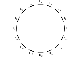
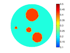
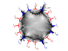
Figure 1. (a) Equispaced geometry of electrodes $E_{l}$ placed over boundary $\partial Q$. (b) True electrical conductivity $\sigma_{true}(x)$. (c) Electrical currents $I_{l}$ (positive in red, negative in blue) injected by electrodes $E_{l}$. Black arrows show the distribution of flux $\sigma(x)\nabla u(x)$ of the electrical potential $u$ in the interior of domain $Q$.

The actual (true) electrical conductivity $\sigma_{true}(x)$ we seek to reconstruct is given analytically by

(6.6) $$\sigma_{true}(x)=\left\{\begin{aligned} &0.4,\qquad&x_{1}^{2}+(x_{2}-0.05)^{2}\leq(0.03)^{2}\\ &0.4,\qquad&(x_{1}+0.075)^{2}+(x_{2}+0.01)^{2}\leq(0.0063)^{2}\\ &0.4,\qquad&(x_{1}+0.015)^{2}+(x_{2}+0.02)^{2}\leq(0.0122)^{2}\\ &0.4,\qquad&(x_{1}-0.025)^{2}+(x_{2}+0.055)^{2}\leq(0.0235)^{2}\\ &0.2,\qquad&\text{otherwise}\end{aligned}\right.$$

measured in $(Ohm\cdot m)^{-1}$ and setting $\sigma_{c}=0.4$ for cancer-affected parts (4 spots of different size) and $\sigma_{h}=0.2$ to healthy tissues parts as seen in Figure 1(b). Electrical currents $I_{l}$ injected by electrodes $E_{l}$ are provided in Table 1 and shown schematically in Figure 1(c). This figure also shows the distribution of flux $\sigma(x)\nabla u(x)$ of the electrical potential $u$ in the interior of domain $Q$ corresponding to $\sigma_{true}(x)$.

Table 1. “Current–to–voltage” model parameters: electrical currents $I_{l}$ injected by electrodes $E_{l},\,l=1,\ldots,16$, with contact impedances $Z_{l}$, and initial guess for boundary voltages $U_{l,ini}$. The unit system used for all values is SI.

Electrode, $l$	1	2	3	4	5	6	7	8	9	10	11	12	13	14	15	16
$I_{l}\cdot 10^{2}$, A	-3	2	3	-7	6	-1	-4	2	4	3	-5	4	3	-5	2	-4
$Z_{l}\cdot 10^{1}$, Ohm	1	1	1	1	1	1	1	1	1	1	1	1	1	1	1	1
$U_{l,ini}$, V	-1	1	-1	1	-1	1	-1	1	-1	1	-1	1	-1	1	-1	1

Our optimization framework integrates computational facilities for solving state PDE problem (6.1)–(6.3), adjoint PDE problem (4.3)–(4.5), and evaluation of the Fréchet gradient according to (4.10), (4.12). These facilities are incorporated by using FreeFem++, see Hecht (2012) for details, an open–source, high–level integrated development environment for obtaining numerical solutions of PDEs based on the Finite Element Method. To numerically solve the state PDE problem (6.1)–(6.3), spatial discretization is carried out by implementing triangular finite elements, P2 piecewise quadratic (continuous) representation for electrical potential $u(x)$ and P0 piecewise constant representation for conductivity field $\sigma(x)$. The system of algebraic equations obtained after such discretization is solved with UMFPACK, a solver for nonsymmetric sparse linear systems. The same technique is used for the numerical solution of adjoint problem (4.3)–(4.5). All computations are performed using 2D domain $Q$ (6.5) which is discretized using mesh $\mathcal{M}(n_{v})$ created by specifying $n_{v}=96$ vertices over boundary $\partial Q$ and totaling 1996 triangular finite elements inside $Q$.

In terms of the initial guess in the iterative algorithm shown in Section 4, unless stated otherwise, we take a constant approximation to (6.6), given by $\sigma_{ini}=\frac{1}{2}\left(\sigma_{h}+\sigma_{c}\right)=0.3$. Initial guess for boundary voltages is provided in Table 1 which is consistent with the ground potential condition (1.2). Determining the Robin part of the boundary conditions in (6.3) we equally set the electrode contact impedance $Z_{l}=0.1$.

The iterative optimization algorithm is performed by the Sparse Nonlinear OPTimizer SNOPT, a software package for solving large-scale nonlinear optimization problems, see Gill et al. (2002). It employs a sparse sequential quadratic programming (SQP) algorithm with limited-memory quasi-Newton approximations to the Hessian of the Lagrangian. This makes SNOPT especially effective for nonlinear problems with computationally expensive functionals and gradients, like in our problem. The termination conditions set for SNOPT are $\left|\frac{\mathcal{J}^{N}-\mathcal{J}^{N-1}}{\mathcal{J}^{N-1}}\right|<10^{-6}$ or maximum number of optimization iterations $N_{max}=250$ whichever comes first.

6.2. Reduced–Dimensional Optimization via PCA–based Re-parameterization

From a viewpoint of numerical optimization, Problem ${\mathcal{J}}$ in its spatially discretized form is over-parameterized even for moderate size models. As previously mentioned in Section 6.1, our 2D computational model requires a solution for 1996-component electrical conductivity vector $\sigma$ when using relatively coarse mesh $\mathcal{M}(96)$. To overcome ill-posedness due to over-parameterization we implement re-parameterization of the control set based on PCA, which is also known as Proper Orthogonal Decomposition (POD) or Karhunen–Loève Expansion.

Without loss of generality, we consider a model which contains $N_{\sigma}$ model parameters. We assume the existence of a set of $N_{r}$ sample solutions (realizations) $\sigma_{j}$, $j=1,\dots,N_{r}$, each of size $N_{\sigma}$. For simplicity we assume a Gaussian (normal) distribution for the model parameters, i.e., $\sigma\sim\mathbb{N}(\bar{\sigma},\mathbb{C}_{M})$, where $\bar{\sigma}=(1/N_{r})\sum_{j=1}^{N_{r}}\sigma_{j}$. Covariance matrix $\mathbb{C}_{M}$ may be approximated by

(6.7) $$\mathbb{C}_{M}\approx\dfrac{XX^{T}}{N_{r}-1},\quad X^{N_{\sigma}\times N_{r}}=\left[\sigma_{1}-\bar{\sigma}\ \ \dots\ \ \sigma_{N_{r}}-\bar{\sigma}\right].$$

It is more efficient to perform singular value decomposition (SVD) on matrix $Y=X/\sqrt{N_{r}-1}$ of size $N_{\sigma}\times N_{r}$, rather than on covariance matrix $\mathbb{C}_{M}$ of size $N_{\sigma}\times N_{\sigma}$, as $N_{r}\ll N_{\sigma}$. The SVD factorization with truncation is then applied to matrix $Y$

(6.8) $$Y\approx\tilde{U}_{N_{\xi}}\,\tilde{\Sigma}_{N_{\xi}}\,\tilde{V}^{T}_{N_{\xi}},$$

where diagonal matrix $\tilde{\Sigma}_{N_{\xi}}$ contains the singular values of $Y$, and matrices $\tilde{U}_{N_{\xi}}$ and $\tilde{V}^{T}_{N_{\xi}}$ are matrices containing the left and right singular vectors of $Y$. More specifically, matrix $\tilde{\Sigma}_{N_{\xi}}$ is truncated to keep only $N_{\xi}$ singular values. Similarly, analogous truncations are applied to $\tilde{U}_{N_{\xi}}$ and $\tilde{V}^{T}_{N_{\xi}}$.

We define a linear transformation

(6.9) $$\Phi^{N_{\sigma}\times N_{\xi}}=\tilde{U}_{N_{\xi}}\,\tilde{\Sigma}_{N_{\xi}},\qquad N_{\xi}\leq N_{\rm min}=\min\{N_{\sigma},N_{r}\}$$

to project the initial control space defined for model parameters $\sigma$ onto reduced-dimensional $\xi$-space which contains only $N_{\xi}$ largest principal components, see Bukshtynov et al. (2015), by means of the unique mapping

(6.10) $$\sigma=\Phi\,\xi+\bar{\sigma}.$$

To construct a “backward” mapping, the simplest approach is to approximate the inverse of matrix $\Phi$, which cannot be inverted due to its size $N_{\sigma}\times N_{\xi}$, using a pseudo-inverse matrix $\hat{\Phi}^{-1}$

(6.11) $$\xi=\Phi^{-1}\,(\sigma-\bar{\sigma})\approx\hat{\Phi}^{-1}\,(\sigma-\bar{\sigma})=\tilde{\Sigma}^{-1}_{N_{\xi}}\,\tilde{U}^{T}_{N_{\xi}}\,(\sigma-\bar{\sigma}).$$

The optimal control problem defined in Section 3 can now be restated in terms of new model parameters $\xi$ used in place of control $\sigma$ as follows

(6.12) $$\left(\hat{\xi},\hat{U}\right)=\underset{\xi,U}{\operatorname{argmin}}\,\mathcal{J}(\xi,U),$$

subject to discretized PDE model (6.1)–(6.3), and using mappings given by (6.10)–(6.11). By applying (6.10) and the chain rule for derivatives, gradient $\nabla_{\xi}\mathcal{J}$ of cost functional $\mathcal{J}$ with respect to controls $\xi$ can be expressed as

(6.13) $$\nabla_{\xi}\mathcal{J}=\Phi^{T}\,\nabla_{\sigma}\mathcal{J}=\tilde{\Sigma}_{N_{\xi}}\,\tilde{U}^{T}_{N_{\xi}}\,\nabla_{\sigma}\mathcal{J}.$$

This expression, in fact, defines projection of gradient $\nabla_{\sigma}\mathcal{J}$ shown in (4.10) from initial (physical) $\sigma$-space onto the reduced-dimensional $\xi$-space. A summary of the discretized finite-dimensional version of the projective gradient method in Besov spaces for the Problem $\mathcal{J}$ outlined in Section 4.1, employing solution of the problem (6.12), is provided in Algorithm 1. The same algorithm could be easily adjusted for solving Problem $\mathcal{I}$ in which case only iteration of $U$ is pursued (see Remarks 4.1 and 5.1).

A problem of approximating covariance matrix $\mathbb{C}_{M}$ in (6.7) to support our current 2D computational model described in Section 6.1 is solved in the following way. A set of $N_{r}=500$ realizations $\sigma_{j}$, $j=1,\dots,N_{r}$, is created using a generator of (uniformly distributed) random numbers. Each realization “contains” from 1 to 7 “cancer-affected” areas with $\sigma_{c}=0.4$. Each area is located randomly within domain $Q$ and represented by a circle of a randomly chosen radius $0<r\leq 0.3r_{Q}$. We refer the discussion on choosing optimal number of principal components $N_{\xi}$ to Appendix B to consider it as a part of a tuning process in optimizing the overall performance of our computational framework.

  $N\leftarrow 0$

  $U^{0}\leftarrow$ initial guess $U_{ini}$

  $\sigma^{0}\leftarrow$ initial guess $\sigma_{ini}$

  construct $\Phi$ and $\hat{\Phi}^{-1}$ by (6.9) and (6.11)

  $\xi^{0}\leftarrow\sigma^{0}$ using (6.11)

  repeat

     given estimate of $(\sigma^{N},U^{N})$, solve state equations (6.1)–(6.3) for $u^{N}$

     given $u^{N}$ and $(\sigma^{N},U^{N})$, solve adjoint equations (4.3)–(4.5) for $\psi^{N}$

     given estimate of $\sigma^{N}$, solve (6.1)–(6.3) for $v_{k}^{N}$ where $U=e_{k}$

     $\left(\nabla_{\sigma}\mathcal{J}(\sigma^{N},U^{N}),\nabla_{U}\mathcal{J}(\sigma^{N},U^{N})\right)\leftarrow\sigma^{N},U^{N},u^{N},\psi^{N}$ by (4.10)

     $\nabla_{\xi}\mathcal{J}(\xi^{N},U^{N})\leftarrow\nabla_{\sigma}\mathcal{J}(\sigma^{N},U^{N})$ by (6.13)

     update $\xi^{N+1}$ and $U^{N+1}$ by using descent directions $D_{\xi}$ and $D_{U}$ obtained from $\nabla_{\xi}\mathcal{J}^{N}$ and $\nabla_{U}\mathcal{J}^{N}$:

(6.14) $$\xi^{N+1}=\xi^{N}-\tau^{N}D_{\xi}\left(\nabla_{\xi}\mathcal{J}(\xi^{N},U^{N})\right)$$

(6.15) $$U^{N+1}=U^{N}-\tau^{N}D_{U}\left(\nabla_{U}\mathcal{J}(\xi^{N},U^{N})\right)$$

     $\sigma^{N+1}\leftarrow\xi^{N+1}$ by (6.10)

     $N\leftarrow N+1$

  until termination criteria are satisfied to a given tolerance

Algorithm 1 Optimization workflow utilizing PCA-based control space re-parameterization

Remark 6.1

Corollary 4.2 in the context of the model example claims that the Fréchet gradient $\mathcal{K}^{\prime}(\sigma,U)\in\textbf{ba}(Q)\times\mathbb{R}^{m}$ is

$$\mathcal{K}^{\prime}(\sigma,U)=\Big{(}\mathcal{K}^{\prime}_{\sigma}(\sigma,U),\mathcal{K}^{\prime}_{U}(\sigma,U)\Big{)}=$$

(6.16) $$\left(-\displaystyle\sum_{j=1}^{m}\nabla u_{j}\cdot\nabla\psi_{j},\Big{(}\displaystyle\sum_{j=1}^{m}\displaystyle\sum_{l=1}^{m}2\Big{[}\int_{E_{l}}\frac{U^{j}_{l}-u_{j}}{Z_{l}}ds-I^{j}_{l}\Big{]}\int_{E_{l}}\frac{\delta_{l,\theta_{kj}}-w^{\theta_{kj}}(s)}{Z_{l}}ds+2\beta(U_{k}-U_{k}^{*})\Big{)}_{k=1}^{m}\right)$$

6.3. Numerical Results for EIT and Inverse EIT Problems

To test the effectiveness of our gradient descent method, we simulate a realistic model example of the inverse EIT problem which adequately represent the diagnosis of the breast cancer in reality. Simulation and computational analysis consists of three stages.

Stage 1. By selecting boundary current pattern $I=(I_{l})_{l=1}^{16}$ we simulate EIT model example with $\sigma=\sigma_{true}$ by solving Problem $\mathcal{I}$ by the gradient descent method described in Section 4.1, Algorithm 1 and identifying optimal control $U_{true}$. Practical analogy of this step is implementation of the “current–to–voltage” procedure: by injecting current pattern $I=(I_{l})_{l=1}^{16}$ on the electrodes $E_{l},\ l=1,\cdots,16$, take the measurement of the voltages $U^{*}=(U^{*}_{1},\cdots,U^{*}_{16})$. In our numerical simulations $U_{true}$ is identified with $U^{*}$.

Numerical result of Stage 1 is demonstrated in a Figure 2. Electrical currents $(I_{l})_{l=1}^{16}$ specified in Table 1 are injected through 16 electrodes $E_{l}$, $l=1,\ldots,16$, and electrical conductivity field $\sigma(x)$ is assumed known, i.e. $\sigma(x)=\sigma_{true}(x)$. Figure 2(a) shows the optimal solution for control $U$ (empty blue circles) reconstructed from the initial guess $U_{l,ini}$ (filled black circles) provided in Table 1. Fast convergence in 6 iterations as seen in Figure 2(b) confirms well-posedness of the EIT Problem and also uniqueness of the global solution $\hat{U}$ of the convex Problem $\mathcal{I}$ (see Remark 5.1).

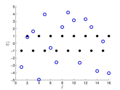
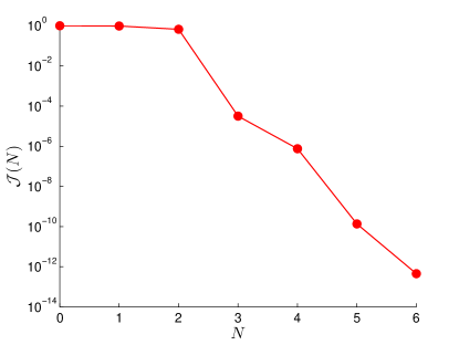
Figure 2. (a) Empty blue circles show optimal solution $\hat{U}$ reconstructed from the initial guess $U_{l,ini}$ (filled black circles) provided in Table 1. (b) Cost functional $\mathcal{I}(N)$ as a function of optimization iteration $N$ in solving the EIT Problem to find optimal solution $(\hat{u}(x),\hat{U})$.

Stage 2. Solve Problem $\mathcal{J}$ with limited data $I=(I_{l})_{l=1}^{16}$ by the gradient descent method described in Section 4.1, Algorithm 1 and to recover optimal control $\left(\sigma_{true},U_{true}\right)$.

Numerical result of Stage 2 without regularization ($\beta=0$) is demonstrated in a Figure 3. Furthermore, in all subsequent Figures, we mark the location of four cancer-affected regions from known $\sigma_{true}$ by dashed circles. As seen in Figure 3(b), the electrical conductivity field $\sigma(x)$ is reconstructed poorly without any signature to identify spots with cancer-affected tissues. Fast convergence with respect to functional in just 6 iterations is demonstrated in Figure 7(a). However, there is no convergence with respect to all control parameters as shown in Figure 3(a,b). Although the $U$-component deviates slightly from actual experimental data $U^{*}$ (filled red circles), the optimal solution $\hat{\sigma}(x)$ obtained for the $\sigma$-component is significantly different from the true solution $\sigma_{true}$. This is a consequence of the ill-posedness of the inverse EIT problem due to non-uniqueness of the solution.

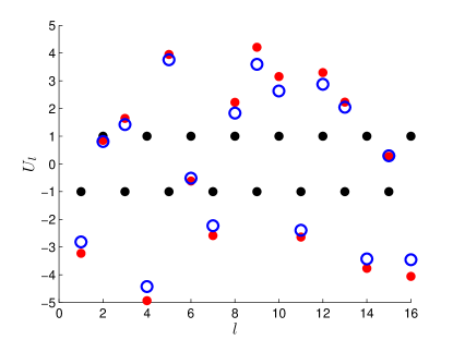
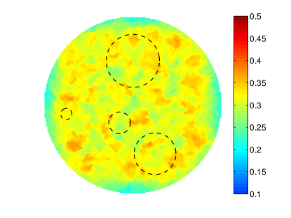
Figure 3. (a) Empty blue circles show optimal solution $\hat{U}$ reconstructed from the initial guess $U_{l,ini}$ (filled black circles) provided in Table 1. Filled red circles represent actual experimental data $U^{*}$ (also blue circles in Figure 2(a)). (b) Reconstructed electrical conductivity field $\hat{\sigma}(x)$. Dashed circles represent the location of four cancer-affected regions taken from known $\sigma_{true}$.

Stage 3. To increase the size of input data we apply the same set of boundary voltages $U^{*}_{l}$ to different electrodes $E_{l}$ using a “rotation scheme”, i.e. we denote $U^{1}=U^{*},I^{1}=I$ and consider 15 new permutations of boundary voltages as in (3.4) applied to electrodes $E_{1},E_{2},\ldots,E_{16}$ respectively. For each boundary voltage vector $U^{j}$ we solve elliptic PDE problem (6.1)–(6.3) to obtain the distribution of electrical potential $u_{j}(\cdot)=u(\cdot;U^{j})$ over boundary $\partial Q$. By using “voltage–to–current” formula (6.4), we calculate current pattern $I^{j}$ associated with $U^{j}$. Thus, a new set $(I^{j})^{16}_{j=1}$ contains 256 input data that could be enough to expect the problem to be well-posed in case a reduced-dimensional space for control $\sigma$ as described in Section 6.2. Practical analogy of this step is implementation of the “voltage–to–current” procedure: by injecting 15 new sets of voltages $U^{j},j=2,...,16$ from (3.4) on the electrodes $E_{l},\ l=1,\cdots,16$, take the measurement of the currents $I^{j}=(I^{j}_{1},\cdots,I^{j}_{16})$. Then we solve Problem $\mathcal{K}$ with extended data set by the gradient descent method described in Section 4.1, Algorithm 1 and to recover optimal control $\left(\sigma_{true},U_{true}\right)$.

Numerical result of Stage 3 without regularization ($\beta=0$) is demonstrated in a Figure 4. Contrary to previous results, the electrical conductivity field $\sigma(x)$ is reconstructed much better matching the two biggest spots while not perfectly capturing their shapes. Reconstruction result for boundary voltage $U$ is also improved.

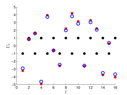
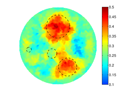
Figure 4. (a) Empty blue circles show optimal solution $\hat{U}$ reconstructed from the initial guess $U_{l,ini}$ (filled black circles) provided in Table 1. Filled red circles represent actual experimental data $U^{*}$ (also blue circles in Figure 2(a)). (b) Reconstructed electrical conductivity field $\hat{\sigma}(x)$. Dashed circles represent the location of four cancer-affected regions taken from known $\sigma_{true}$.

Finally, we evaluate the effect of adding regularization term ($\beta>0$) in the cost functional (3.5). The outcomes with respect to different values of regularization parameter $\beta$ (blue dots) are shown in Figure 5(a). The dashed line represents the result of optimization with $\beta=0$. Numerical results demonstrate that small values of $\beta$ (roughly when $\beta<10^{-4}$) have no significant effect towards decreasing the values of the cost functional $\mathcal{K}$. Significant improvement at different scales is observed when $\beta>10^{-1}$. To identify optimal value for $\beta$, we examine additionally $\sigma$ and $U$ solution norms $N_{\sigma}=\frac{\|\sigma-\sigma_{true}\|_{L_{2}}}{\|\sigma_{true}\|_{L_{2}}}$ and $N_{U}=\frac{|U-U^{*}|}{|U^{*}|}$ presented in Figure 5(b). Based on the numerical results, we pick up the value (shown by hexagons) $\beta^{*}=0.3162$ as the best value in terms of improvement of solutions simultaneously with respect to both controls $\sigma$ and $U$. Figure 6 shows optimal solution $(\hat{\sigma}(x),\hat{U})$ obtained by choosing $\beta^{*}=0.3162$. Overall optimization performance in the last case is also enhanced by much faster convergence. Figure 7(b) provides the comparison for convergence results obtained for two different cases, namely without regularization (blue dots), and with regularization with parameter $\beta^{*}=0.3162$ (red dots).

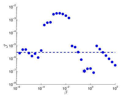
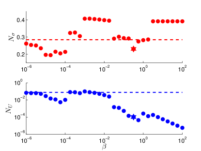
Figure 5. (a) Cost functional $\mathcal{K}$ values and (b) solution norms $N_{\sigma}=\frac{\|\sigma-\sigma_{true}\|_{L_{2}}}{\|\sigma_{true}\|_{L_{2}}}$ and $N_{U}=\frac{|U-U^{*}|}{|U^{*}|}$ evaluated at termination (dots) for different values of regularization parameter $\beta$ in (3.1) and (dashed lines) when $\beta=0$. The best results obtained at $\beta^{*}=0.3162$ are shown by hexagons.

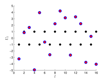
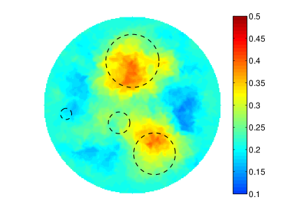
Figure 6. (a) Empty blue circles show optimal solution $\hat{U}$ reconstructed from the initial guess $U_{l,ini}$ (filled black circles) provided in Table 1. Filled red circles represent actual experimental data $U^{*}$ (also blue circles in Figure 2(a)). (b) Reconstructed electrical conductivity field $\hat{\sigma}(x)$. Dashed circles represent the location of four cancer-affected regions taken from known $\sigma_{true}$. Optimal solution $(\hat{\sigma}(x),\hat{U})$ is obtained by solving the Problem $\mathcal{K}$ with regularization parameter $\beta^{*}=0.3162$ in (3.5).

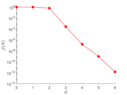
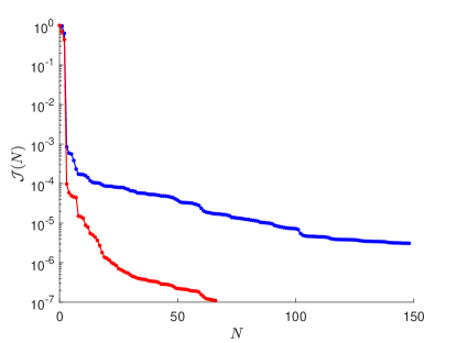
Figure 7. Cost functional $\mathcal{J}(N)$ as a function of optimization iteration $N$ in solving the EIT Inverse Problem to find optimal solution $(\hat{\sigma}(x),\hat{U})$ (a) without and (b) with applying additional data acquired through rotating boundary voltages $U_{l}$. Convergence in (b) is compared for two cases: (blue dots) without regularization, and (red dots) when applying regularization with parameter $\beta^{*}=0.3162$.

7. Conclusions

This paper analyzes the inverse EIT problem on recovering electrical conductivity tensor and potential in the body based on the measurement of the boundary voltages on the electrodes for a given electrode current. The inverse EIT problem presents an effective mathematical model of breast cancer detection based on the experimental fact that the electrical conductivity of malignant tumors of the breast may significantly differ from conductivity of the surrounding normal tissue. We analyze the inverse EIT problem in a PDE constrained optimal control framework in Besov space, where the electrical conductivity tensor and boundary voltages are control parameters, and the cost functional is the norm declinations of the boundary electrode current from the given current pattern and boundary electrode voltages from the measurements. The state vector is a solution of the second order elliptic PDE in divergence form with bounded measurable coefficients under mixed Neumann/Robin type boundary condition. The following are the main results of the paper:

• In contrast with the current state of the field, the inverse EIT problem is investigated with unknown electrical conductivity tensor, which is essential in understanding and detecting the highly anisotropic distribution of cancerous tumors in breast tissue.

• To address the highly ill-posed nature of the inverse EIT problem, we develop a ”variational formulation with additional data” which is well adapted to clinical situation when additional “voltage–to–current” measurements significantly increase the size of the input data while keeping the size of the unknown parameters fixed.

• Existence of the optimal control and Fréchet differentiability in the Besov space setting is proved. The formula for the Fréchet gradient and optimality condition is derived. Effective numerical method based on the projective gradient method in Besov spaces is developed.

• Extensive numerical analysis is pursued in the 2D case through implementation of the projective gradient method, re-parameterization via PCA, and Tikhonov regularization in a carefully constructed model example which adequately represents the diagnosis of breast cancer in reality. Numerical analysis demonstrates accurate reconstruction of the electrical conductivity function of the body in the frame of the model based on ”variational formulation with additional data”.

Appendices

A. Validation of Gradients

In this section we present results demonstrating the consistency of cost functional gradients $\nabla_{\sigma}\mathcal{J}$, $\nabla_{\xi}\mathcal{J}$ and $\nabla_{U}\mathcal{J}$ obtained with the approach described in Section 4 and Algorithm 1. As the sensitivity of cost functionals $\mathcal{J}(\sigma,U)$ and $\mathcal{J}(\xi,U)$ with respect to controls may vary significantly for different contributions of $\sigma$, $\xi$ and $U$, it is reasonable to perform testing separately for different parts of the gradients, namely $\nabla_{\sigma}\mathcal{J}(\sigma,U)$, $\nabla_{\xi}\mathcal{J}(\xi,U)$ and $\nabla_{U}\mathcal{J}(\sigma,U)$.

First, we explore the results obtained for controls representing electrical conductivity $\sigma$ before and after projecting the gradients onto the reduced-dimensional $\xi$-space as described in Section 6.2. Figure A.1 shows the results of a diagnostic test commonly employed to verify correctness of cost functional gradients (see, e.g., Bukshtynov et al. (2011), Bukshtynov & Protas (2013)) computed for our computational model detailed in Section 6.1. Testing $\nabla_{\sigma}\mathcal{J}(\sigma,U)$ consists in computing the Fréchet differential $d\mathcal{J}(\sigma,U;\delta\sigma)=\left\langle{}\mathcal{J}^{\prime}(\sigma,U),{\delta\sigma}\right\rangle_{H}$ for some selected variations (perturbations) $\delta\sigma$ in two different ways, namely, using a finite–difference approximation and using (4.10) which is based on the adjoint field, and then examining the ratio of the two quantities, i.e.,

(A.1) $$\kappa(\epsilon)=\dfrac{\frac{1}{\epsilon}\left[\mathcal{J}(\sigma+\epsilon\,\delta\sigma,U)-\mathcal{J}(\sigma,U)\right]}{\left\langle{}\mathcal{J}^{\prime}(\sigma,U),{\delta\sigma}\right\rangle_{H}}$$

for a range of values of $\epsilon$. If these gradients are computed correctly, then for intermediate values of $\epsilon$, $\kappa(\epsilon)$ will be close to the unity. Remarkably, this behavior can be observed in Figure A.1(a) over a range of $\epsilon$ spanning about 8-9 orders of magnitude for controls $\sigma$. Furthermore, we also emphasize that refining mesh $\mathcal{M}(n_{v})$ in discretizing domain $Q$ while solving both state (6.1)–(6.3) and adjoint (4.3)–(4.5) PDE problems yields values of $\kappa(\epsilon)$ closer to the unity. The reason is that in the “optimize–then–discretize” paradigm adopted here such refinement of discretization leads to a better approximation of the continuous gradient as shown in Protas et al. (2004). We add that the quantity $\log_{10}|\kappa(\epsilon)-1|$ plotted in Figure A.1(b) shows how many significant digits of accuracy are captured in a given gradient evaluation. As can be expected, the quantity $\kappa(\epsilon)$ deviates from the unity for very small values of $\epsilon$, which is due to the subtractive cancelation (round–off) errors, and also for large values of $\epsilon$, which is due to the truncation errors, both of which are well–known effects.

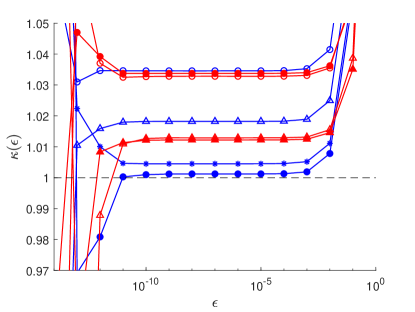
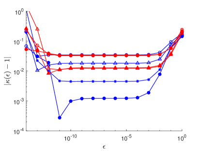
Figure A.1. The behavior of (a) $\kappa(\epsilon)$ and (b) $\log_{10}|\kappa(\epsilon)-1|$ as a function of $\epsilon$ for both controls (blue) $\sigma(x)$ and (red) $\xi$. Number of vertices over boundary $\partial Q$ used in spatial discretization of domain $Q$ for computing $\nabla_{\sigma}\mathcal{J}(\sigma,U)$ are (open circles) $n_{v}=48$ (724 mesh $\mathcal{M}$ triangular finite elements), (triangles) $n_{v}=96$ (1996 elements), (asterisks) $n_{v}=176$ (7800 elements), (filled circles) $n_{v}=432$ (47938 elements). Same meshes (red circles) $\mathcal{M}(48)$ and (red triangles) $\mathcal{M}(96)$ are used for computing $\nabla_{\xi}\mathcal{J}(\xi,U)$ with number of principal components (open circles/triangles) $N_{\xi}=20$ and (filled circles/triangles) $N_{\xi}=74$.

The same test could be easily applied for controls $\xi$ to check the consistency for gradients $\nabla_{\xi}\mathcal{J}(\xi,U)$ in the reduced-dimensional $\xi$-space. As seen in Figure A.1 the same conclusion could be made on the effect of refining mesh $\mathcal{M}(n_{v})$ in discretizing domain $Q$. We should notice that applying PCA-based re-parameterization improves the results of this diagnostics. At the same time we conclude that changing number of principal components $N_{\xi}$ influences the results of the test insignificantly. This effect is easily explained by the fact that only the first, and thus the biggest, components have sufficient weight and prevails over the rest components in the truncated tail of the PCA-component sequence.

Second, we could also apply the same testing technique to check the correctness and consistency for gradients $\nabla_{U}\mathcal{J}(\sigma,U)$ as shown in Figure A.2(a). Unlike for tests performed for controls $\sigma$ and $\xi$, gradients $\nabla_{U}\mathcal{J}(\sigma,U)$ are computed correctly but with much larger error demonstrated by the plateau form of $\kappa(\epsilon)$ which is quite distant from the unity. Remarkably, refining mesh $\mathcal{M}(n_{v})$ in discretizing domain $Q$ while solving both state (6.1)–(6.3) and adjoint (4.3)–(4.5) PDE problems does not change significantly the quality of the obtained gradients with respect to controls $U$. We explain this by the fact that computing gradients $\nabla_{U}\mathcal{J}(\sigma,U)$ relies mainly on the solution for the potential $u(x)$ obtained on or very close to boundary $\partial Q$ where it looses its regularity due to discontinuous boundary conditions (6.2)–(6.3). As control vector $U$ contains only $m=16$ components, we could also perform our diagnostic test applied individually to every component $U_{l}$ for fixed (intermediate) value of $\epsilon$

(A.2) $$\kappa(l)=\dfrac{\frac{1}{\epsilon}\left[\mathcal{J}(\sigma,U_{l}+\epsilon\,\delta U_{l})-\mathcal{J}(\sigma,U_{l})\right]}{\mathcal{J}^{\prime}(\sigma,U_{l})\cdot\delta U_{l}}.$$

Figure A.2(b) represents the results of this modified test which may also be used in analysis for sensitivity of cost functional $\mathcal{J}(\sigma,U)$ to changes in boundary potential $U_{l}$ at individual electrode $E_{l}$.

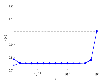
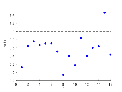
Figure A.2. (a) The behavior of $\kappa(\epsilon)$ as a function of $\epsilon$ for control $U$. Number of vertices over boundary $\partial Q$ used in spatial discretization of domain $Q$ for computing $\nabla_{U}\mathcal{J}(\sigma,U)$ are (triangles) $n_{v}=96$ (1996 mesh $\mathcal{M}$ triangular finite elements), (asterisks) $n_{v}=176$ (7800 elements), (filled circles) $n_{v}=432$ (47938 elements). (b) The behavior of $\kappa(l)$ as a function of electrode number $l$ for control $U$ computed by (A.2).

B. Optimal Size of Reduced-Dimensional $\xi$-space

In this section we provide a discussion on choosing optimal number of principal components $N_{\xi}$ to reduce dimensionality of the solution space for control $\sigma$ as discussed previously in Section 6.2 in order to optimize overall performance of our computational framework. Following this discussion, a set of $N_{r}=500$ realizations $\sigma_{j}$ is used to construct linear transformation matrix $\Phi^{N_{\sigma}\times N_{\xi}}$ in (6.9) based on truncated SVD factorization of matrix $Y$. Figure B.1(a) shows the first 400 out of 500 eigenvalues $\lambda_{k}$ of matrix $Y$.

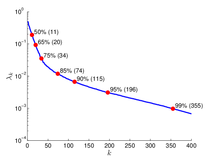
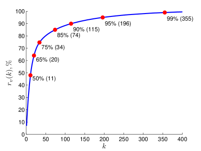
Figure B.1. (a) The values the of first 400 out of 500 eigenvalues $\lambda_{k}$ of matrix $Y$ obtained from a set of $N_{r}=500$ realizations $\sigma_{j}$. (b) Accumulated portion $r_{v}(k)$ of the variance (energy) contained in eigenvalues $\lambda_{1}$ through $\lambda_{k}$ as a function of $k$. For both graphs numbers in parentheses are the numbers $k$ of eigenvalues ($\lambda_{1},\ldots,\lambda_{k}$) contained in the portion $r_{v}$ of the accumulated variance.

Various approaches can be used to determine the size of the $\xi$-space; i.e., the $N_{\xi}$ value. Options include the Kaiser criterion $\lambda\geq 1$ shown in Kaiser (1960), the scree test introduced in Cattell (1966), and the inclusion of a prescribed portion $r_{v}$ of the variance (energy) contained in eigenvalues $\lambda_{1}$ through $\lambda_{k}$ shown in Figure B.1(b). With this last approach, given the (prescribed) parameter $r_{\rm opt}$, $N_{\xi}$ is determined such that the following condition is satisfied

(B.1) $$r_{v}(N_{\xi})=\dfrac{\sum_{i=1}^{N_{\xi}}\lambda_{i}}{\sum_{i=1}^{N_{\rm min}}\lambda_{i}}\cdot 100\%\geq r_{\rm opt}.$$

The scree test returns the value $r_{v}$ close to 80%–85% as at this values the graph of $r_{v}(k)$ is bending. To determine parameter $r_{\rm opt}$ we run our 2D model described in Section 6.1 multiple times changing the size of the $\xi$-space by setting $r_{v}$ value in (B.1) to different numbers within the range from $15\%(N_{\xi}=2)$ to $100\%(N_{\xi}=495)$ with step $5\%$. The performance is evaluated first by examining cost functional $\mathcal{J}$ values at termination for three different cases to restart limited-memory quasi-Newton approximations for Hessian in SNOPT: every $N=1,5,10$ iterations. The outcomes are represented respectively by blue, red and green dots in Figure B.2(a). The results of two cases with restarts every 5 and 10 iterations are consistent with the scree test. We additionally examine $\sigma$ and $U$ solution norms $N_{\sigma}=\frac{\|\sigma-\sigma_{true}\|_{L_{2}}}{\|\sigma_{true}\|_{L_{2}}}$ and $N_{U}=\frac{|U-U^{*}|}{|U^{*}|}$ with results for $N=5$ presented in Figure B.2(b). This test reveals the optimal value for $r_{v}$ to be close to 65% providing only $N_{\xi}=20$ dimensions for $\xi$-space. This creates a high possibility for $\xi$ control space to be under-parameterized. Therefore, for all computations shown in Section 6.3, unless stated otherwise, we used $N_{\xi}=74$ utilizing $r_{opt}=85\%$ of accumulated variance.

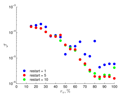
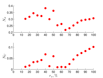
Figure B.2. (a) Cost functional $\mathcal{J}$ values evaluated at termination when Hessian approximations are restarted every (blue dots) $N=1$, (red dots) $N=5$, and (green dots) $N=10$ iterations. (b) Solution norms $N_{\sigma}$ and $N_{U}$ evaluated at termination for case $N=5$.

References

- (1)
- Abdulla (2013) Abdulla, U. G. (2013), ‘On the optimal control of the free boundary problems for the second order parabolic equations. I. Well-posedness and convergence of the method of lines’, Inverse Problems and Imaging 7(2), 307–340.
- Abdulla (2016) Abdulla, U. G. (2016), ‘On the optimal control of the free boundary problems for the second order parabolic equations. II. Convergence of the method of finite differences’, Inverse Problems and Imaging 10(4), 869–898.
- Abdulla et al. (2019) Abdulla, U. G., Bukshtynov, V. & Hagverdiyev, A. (2019), ‘Gradient method in Hilbert-Besov spaces for the optimal control of parabolic free boundary problems’, Journal of Computational and Applied Mathematics 346, 84–109.
- Abdulla et al. (2017) Abdulla, U. G., Cosgrove, E. & Goldfarb, J. (2017), ‘On the Fréchet differentiability in optimal control of coefficients in parabolic free boundary problems’, Evolution Equations and Control Theory 6(4), 319–344.
- Abdulla & Goldfarb (2018) Abdulla, U. G. & Goldfarb, J. M. (2018), ‘Fréchet differentiability in Besov spaces in the optimal control of parabolic free boundary problems’, Journal of Inverse and Ill-posed Problems 26(2), 211–227.
- Adler et al. (n.d.) Adler, A., Arnold, J., Bayford, R., Borsic, A., Brown, B., Dixon, P., Faes, T. J., Frerichs, I., Gagnon, H., Gärber10, Y. et al. (n.d.), ‘GREIT: towards a consensus EIT algorithm for lung images’.
- Adler & Lionheart (2005) Adler, A. & Lionheart, W. R. (2005), EIDORS: towards a community-based extensible software base for EIT, in ‘6th Conf. on Biomedical Applications of Electrical Impedance Tomography’, pp. 1–4.
- Alessandrini (1988) Alessandrini, G. (1988), ‘Stable determination of conductivity by boundary measurements’, Applicable Analysis 27(1-3), 153–172.
- Besov et al. (1979a) Besov, O. V., Il’in, V. P. & Nikol’skii, S. M. (1979a), Integral Representations of Functions and Imbedding Theorems, Vol. Vol. 1, John Wiley & Sons.
- Besov et al. (1979b) Besov, O. V., Il’in, V. P. & Nikol’skii, S. M. (1979b), Integral Representations of Functions and Imbedding Theorems, Vol. Vol. 2, John Wiley & Sons.
- Borcea (2002) Borcea, L. (2002), ‘Electrical impedance tomography’, Inverse Problems 18, 99–136.
- Brown (2003) Brown, B. H. (2003), ‘Electrical impedance tomography (EIT): A review’, Journal of medical engineering & technology 27(3), 97–108.
- Bukshtynov & Protas (2013) Bukshtynov, V. & Protas, B. (2013), ‘Optimal reconstruction of material properties in complex multiphysics phenomena’, Journal of Computational Physics 242, 889–914.
- Bukshtynov et al. (2015) Bukshtynov, V., Volkov, O., Durlofsky, L. & Aziz, K. (2015), ‘Comprehensive framework for gradient-based optimization in closed-loop reservoir management’, Computational Geosciences 19(4), 877–897.
- Bukshtynov et al. (2011) Bukshtynov, V., Volkov, O. & Protas, B. (2011), ‘On optimal reconstruction of constitutive relations’, Physica D: Nonlinear Phenomena 240(16), 1228–1244.
- Calderon (1980) Calderon, A. (1980), On an inverse boundary value problem, in ‘Seminar on Numerical Analysis and Its Applications to Continuum Physics’, Soc. Brasileira de Mathematica, Rio de Janeiro, pp. 65–73.
- Cattell (1966) Cattell, R. B. (1966), ‘The scree test for the number of factors’, Multivariate Behavioral Research 1(2), 245–276.
- Cheng et al. (1989) Cheng, K.-S., Isaacson, D., Newell, J. & Gisser, D. G. (1989), ‘Electrode models for electric current computed tomography’, IEEE Transactions on Biomedical Engineering 36(9), 918–924.
- Demidenko (2011) Demidenko, E. (2011), ‘An analytic solution to the homogeneous EIT problem on the 2D disk and its application to estimation of electrode contact impedances’, Physiological measurement 32(9), 1453.
- Demidenko et al. (2011) Demidenko, E., Borsic, A., Wan, Y., Halter, R. J. & Hartov, A. (2011), ‘Statistical estimation of EIT electrode contact impedance using a magic Toeplitz matrix’, IEEE Transactions on Biomedical Engineering 58(8), 2194–2201.
- Dunlop & Stuart (2016) Dunlop, M. M. & Stuart, A. M. (2016), ‘The Bayesian formulation of EIT: analysis and algorithms’, Inverse Problems and Imaging 10(4), 1007–1036.
- Evans (1998) Evans, L. (1998), Partial Differential Equations, Graduate studies in mathematics, American Mathematical Society.
- Gill et al. (2002) Gill, P. E., Murray, W. & Saunders, M. (2002), ‘SNOPT: An SQP algorithm for large-scale constrained optimization’, SIAM Journal on Optimization 12(4), 979–1006.
- Hecht (2012) Hecht, F. (2012), ‘New development in FreeFem++’, J. Numer. Math. 20(3-4), 251–265.
- Holder (2004) Holder, D. S. (2004), Electrical impedance tomography: methods, history and applications, CRC Press.
- Kaipio et al. (2000) Kaipio, J. P., Kolehmainen, V., Somersalo, E. & Vauhkonen, M. (2000), ‘Statistical inversion and Monte Carlo sampling methods in electrical impedance tomography’, Inverse problems 16(5), 1487.
- Kaipio et al. (1999) Kaipio, J. P., Kolehmainen, V., Vauhkonen, M. & Somersalo, E. (1999), ‘Inverse problems with structural prior information’, Inverse problems 15(3), 713.
- Kaiser (1960) Kaiser, H. F. (1960), ‘The application of electronic computers to factor analysis’, Educational and Psychological Measurement 20(1), 141–151.
- Kenig et al. (2007) Kenig, C., Sjöstrand, J. & Uhlmann, G. (2007), ‘The Calderon problem with partial data’, Annals of Mathematics 165, 567–591.
- Nachman (1988) Nachman, A. I. (1988), ‘Reconstructions from boundary measurements’, Annals of Mathematics 128(3), 531–576.
- Nikol’skii (1975) Nikol’skii, S. M. (1975), Approximation of Functions of Several Variables and Imbedding Theorems, Springer-Verlag, New York-Heidelberg.
- Paulson et al. (1995) Paulson, K., Lionheart, W. & Pidcock, M. (1995), ‘POMPUS: an optimized EIT reconstruction algorithm’, Inverse Problems 11(2), 425.
- Protas et al. (2004) Protas, B., Bewley, T. & Hagen, G. (2004), ‘A computational framework for the regularization of adjoint analysis in multiscale PDE systems’, Journal of Computational Physics 195(1), 49–89.
- Roininen et al. (2014) Roininen, L., Huttunen, J. M. & Lasanen, S. (2014), ‘Whittle-Matérn priors for Bayesian statistical inversion with applications in electrical impedance tomography’, Inverse Probl. Imaging 8(2), 561–586.
- Somersalo et al. (1992) Somersalo, E., Cheney, M. & Isaacson, D. (1992), ‘Existence and uniqueness for electrode models for electric current computed tomography’, SIAM Journal on Applied Mathematics 52(4), 1023–1040.
- Sylvester & Uhlmann (1987) Sylvester, J. & Uhlmann, G. (1987), ‘A global uniqueness theorem for an inverse boundary value problem’, Annals of mathematics pp. 153–169.
- Zou & Guo (2003) Zou, Y. & Guo, Z. (2003), ‘A review of electrical impedance techniques for breast cancer detection’, Medical Engineering and Physics 25(2), 79–90.