Late time supernova neutrino signal
and proto-neutron star radius

Abstract

We discuss the possibility of reconstructing the newly formed proto-neutron star radius from the late time neutrino signal. A black-body emission is assumed for the neutron star cooling phase. We parametrize the neutrino time-integrated fluxes based on simulations of Roberts and Reddy. A likelihood analysis of the inverse-beta decay and elastic scattering events in Hyper-Kamiokande is performed in both three flavor and an effective one flavor scenario. We show that the precision achievable in the radius reconstruction strongly depends on a correlation with the pinching parameter and therefore the corresponding prior. Although this correlation hinders the precise measurement of the newly formed neutron star radius, it could help measure the pinching parameters with good accuracy in view of the current constraints on neutron star radius, or if the neutron star radius is precisely measured.

1 Introduction

Neutrinos from core-collapse supernovae are an incomparable laboratory for astroparticle physics. The measurement of the neutrino luminosity curves from future galactic explosions is fundamental to fully unravel the explosion mechanism, to pin down the newly born neutron-star or exotic neutrino properties and to tell us about neutrino flavor conversion in dense and explosive environments. The delayed explosion mechanism aided by the standing accretion shock instability is thought to be responsible for the vast majority of core-collapse supernovae [1]. Imprints of such an instability are expected to be present in the neutrino time signal and be detectable in IceCube [2]. In addition, Colgate and Johnson hypothesized that the gravitational binding energy of the newly formed neutron star is taken away by electron, muon and tau neutrinos and antineutrinos [3]. This conjecture, supported by the analyses of SN1987A observations under the equipartition assumption (see e.g. [4, 5, 6]) will be precisely verified by the future measurement of the gravitational binding energy of the newly formed neutron star in Super-Kamiokande at $11\%$ [7] and in Hyper-Kamiokande at $3\%$ percent level [8].

Concerning the exotic neutrino properties, neutrino flavor transformations have been reliably studied only on relatively small distances. This circumstance does not allow us to exclude firmly the possibility that new phenomena occur when neutrinos travel on cosmic scales — thus leading to major modifications of the supernova neutrino signal. This was first discussed in the context of the models in which the neutrino mass is supposed to have pseudo-Dirac character, namely, those models where left and right neutrinos exist (see [9, 10] and references therein). Certain models for sterile neutrinos, based on the hypothesis of exact mirror symmetry, have slightly stronger theoretical and phenomenological bases. They provide us, for instance, with convincing candidates for dark matter particles (see e.g. [11]) and lead to very different masses for neutrinos. However, they lead to the same phenomenology for what concerns neutrino oscillations. In fact, it was argued that a rather interesting case for vacuum oscillations on cosmic scales, is the one when the disappearance of the ordinary neutrinos results in just half of the original flux in the case of mirror neutrinos [12] or for pseudo-Dirac neutrinos [13]. The electron antineutrinos observed from SN 1987A do not exclude this possibility strongly [14].

The neutrino signal from a future core-collapse supernova will also provide us with information on other macroscopic properties of the newly formed neutron star, in particular its mass and radius, just as in the case of SN 1987A [4]. Observationally, constraints on mass and radius of the neutron star, and consequently on its equation of state can be obtained by Bayesian analyses of quiescent low mass X-ray binaries [15]. The NICER experiment will measure the mass-radius relation as well as the radius itself through the timing and the spectroscopy of thermal and non-thermal emission of neutron stars in the soft X-ray band [16]. The expected sensitivity is at the level of $5\%$ precision on the radii and will furnish tight observational constraints on the neutron star equation of state. As for the neutron star masses, they are precisely measured in radio binary pulsars or in X-ray accreting binaries (see [17] for a compilation of measurements). In addition, gravitational waves constitute a powerful probe for neutron star properties and for extended theories of gravity. The recent measurement of gravitational waves from binary neutron stars has indeed yielded information on the neutron star mass-radius relation and the equation of state [18].

A question one might ask is “what would be the prospects on measuring the radius of the nascent neutron star in the future measurement of a supernova neutrino time signal”. This determination would rely on reference models for the time signal, or the fluences. Moreover theoretical information would be needed to establish the connection between the neutrinosphere and the neutron star radii.

In the present manuscript we address the issue of the reconstruction of the neutron star radius under the assumption of a black body emission from the nascent neutron star. We consider neutrino fluences from the simulations of Reddy and Roberts as a template. In our investigation, we study the signal observed in Hyper-Kamiokande, the largest water Cherenkov detector currently under consideration. We combine inverse beta decay and elastic scattering detection channels and perform several nine-degrees of freedom likelihood analyses. The total energy, the average energy and the pinching parameters that characterize the neutrino fluences for the three neutrino species can vary within their priors and are reconstructed using the simulated data. We show that the inclusion of the pinching parameters which quantify the deviations from the thermal distribution significantly affects the results of the analysis.

We perform three analyses in which we employ different priors for the pinching parameter. Moreover, we consider a supernova explosion at $2\text{\,}\mathrm{kpc}$ and at $10\text{\,}\mathrm{kpc}$ as reference distances. We discuss the precision in the neutron star radius reconstruction and the difficulties inherent to it. Finally, we analyze the possibility to determine the pinching parameter of the neutrino fluences by implementing reasonable ansatz on the neutron star radius.

The manuscript is structured as follows. In section 2 we introduce the hypothesis assumed for the neutrino emission from the nascent neutron star, the time integrated neutrino fluxes and their flavor modification. Section 3 presents the likelihood analyses performed in Hyper-Kamiokande. Our numerical results concerning the reconstruction of the neutron star radius from the neutrino time signal is presented in section 4. The possibility to determine the pinching parameter from the neutrino fluences is also discussed. Section 5 is devoted to conclusions.

2 Neutrino time signal and proto-neutron star cooling

2.1 Parameterization of the cooling phase time signal

During the proto-neutron star cooling phase, the neutrino emission can be approximately described by a black-body of luminosity $L$ characterized by temperature $T$ and radius $R$

$$L=4\pi\sigma_{\text{{bb}}}\phi(\eta)R^{2}\,k_{B}^{4}T^{4},$$ (1)

where $\eta$ is the pinching parameter and $\sigma_{\text{{bb}}}$ is the black body constant for a species with one degree of freedom following a perfect Maxwell-Boltzmann distribution

$$\sigma_{\text{{bb}}}=\frac{45}{\pi^{4}}\times\frac{2\pi^{5}}{15c^{2}h^{3}}\approx$4.75\text{\times}{10}^{35}\text{\,}\mathrm{erg}\text{\,}{\mathrm{MeV}}^{-4}\text{\,}{\mathrm{cm}}^{-2}\text{\,}{\mathrm{s}}^{-1}$.$$ (2)

The parameter $\phi$, of the order of unity, accounts for deviations from such distribution.

Equation (1) can be used to reconstruct the neutron star radius $R$, once the neutrino flux parameters $L$, $T$, $\eta$ are known. In the present work we consider as reference the output of the detailed simulations by Roberts and Reddy [19]. Such simulations extend up to several seconds after core-bounce where the neutrino emission is believed to be related to the quasi-static Helmholtz cooling of the proto-neutron star [20]. Figure 3 of ref. [19] shows that the time evolution of the flux parameters and the neutrinosphere radii $R_{\nu,i}$, are quite constant at later times for the three neutrino species, $\nu_{\mathrm{e}}$, $\overline{\nu}_{\mathrm{e}}$ and $\nu_{x}$. Hence, in order to define a neutron-star radius we consider the time window from $6\text{\,}\mathrm{s}$ to $10\text{\,}\mathrm{s}$. We note that the neutrinospheres that depend both on the neutrino flavor and energy are defined as the location where the opacity is equal to $2/3$ — as in ref. [19]. Since the neutron star radius is supposed to be close to the neutrinosphere locations within $10\%$ [4, 19], in our analysis we consider the neutron star radius to be at the same location as the neutrinosphere radius.

The time-dependent (isotropic) neutrino fluxes at the neutrinospheres $\Phi_{i}^{0}$ are given by

$$\frac{\partial^{2}\Phi_{i}^{0}}{\partial E\partial t}=\frac{\dot{N}_{\nu,i}^{t}}{4\pi{D}^{2}}f_{i}(E,t)\quad\text{with}\quad i=\nu_{\mathrm{e}},\,\overline{\nu}_{\mathrm{e}}\,\nu_{x},$$ (3)

where $\dot{N}_{\nu,i}^{t}=L^{t}_{i}/\langle E_{i}\rangle^{t}$ is the number of emitted neutrinos per unit time, the superscript $t$ recalls that we are dealing with time-dependent quantities and $D$ is the supernova distance. The $f_{i}(E,t)$ functions parameterize the energy distribution for each species, normalized to 1. In the simulation [19], Fermi-Dirac distributions are considered

$$f_{i}\left(E,t\right)=\frac{E^{2}}{(k_{B}T_{i}^{t})^{3}\,F_{2}(\eta_{i}^{t})}\left[1+\exp\left(\frac{E}{k_{B}T_{i}^{t}}-\eta_{i}^{t}\right)\right]^{-1}$$ (4)

where the temperatures are related to the mean energies $\langle E_{i}\rangle^{t}$ through

$$k_{B}T_{i}^{t}=\frac{\left\langle E_{i}\right\rangle^{t}F_{2}(\eta_{i}^{t})}{F_{3}(\eta_{i}^{t})}.$$ (5)

The $F_{n}\left(\eta\right)$ are the Fermi functions

$$F_{n}(\eta)=\int_{0}^{\infty}\frac{x^{n}\operatorname{d}\!{x}}{1+\exp\left(x-\eta\right)}=-\,n!\>\mathrm{Li}_{n+1}\left(-e^{\eta}\right).$$ (6)

From considerations of statistical mechanics one can derive the expression of the flux from a spherically symmetric source emitting fermions — see e.g. [21]

$$\frac{\operatorname{d}\!{\Phi}_{\nu}^{\text{{sm}}}}{\operatorname{d}\!{E}}=\frac{\pi R^{2}c}{4\pi D^{2}}\frac{4\pi E^{2}}{c^{3}h^{3}}\left[1+\exp\left(\frac{E}{k_{B}T}-\eta\right)\right]^{-1}.$$ (7)

Notice that, here $\eta$ is not related to a chemical potential [22]. Comparing equations (3) and (7) we obtain an explicit relation that links the luminosity $L_{i}^{t}$, the radius $R_{i}^{t}$, the temperature $T_{i}^{t}$ and the pinching $\eta_{i}^{t}$

$$L_{i}^{t}=-\frac{24\pi^{2}c}{\left(hc\right)^{3}}\left(R_{i}^{t}\right)^{2}\left(k_{B}T_{i}^{t}\right)^{4}\mathrm{Li}_{4}(-e^{\eta_{i}^{t}}).$$ (8)

This expression constitutes the black-body law we will consider for the neutrino emission. Note that the effect of departures from an exactly thermal emission are included in this formula by the corrections introduced by the pinching parameter.

In principle, the reconstruction of the neutron-star radius would require 12 degree time-dependent likelihood analysis — $L_{i}^{t}$, $\langle E\rangle^{t}$, $\eta_{i}^{t}$ and $R_{i}^{t}$, satisfying equation (8). According to the results of ref. [19] (figure 3), the quantities $L_{i}^{t}$, $\langle E\rangle^{t}$ and $R_{i}^{t}$ are quite constant in the chosen time window. The pinching parameter can be deduced from equation (8) in terms of the luminosity, average energy and radius at each time. Obviously, $\eta_{i}^{t}$ turns out to be approximately time independent as well. As a consequence, we do not work with instantaneous fluxes but instead we integrate equation (3) over time to obtain fluences. We will then be dealing with effective $L_{i}$, $\langle E\rangle$ and $\eta$. From these quantities and by using equation (8), we reconstruct $R_{i}$ that will also be an effective parameter.

Another justification to the time-independent likelihood analysis we perform is that a precise determination requires a large statistics, for which the supernova location $D$ is a key parameter. For the typical value $D=$10\text{\,}\mathrm{kpc}$$ corresponding to the mean of the core-collapse supernova distribution in our Galaxy [23] and in a restricted time window for the neutrino signal, the luminosities have already fainted considerably. As we will show (section 3), the number of expected events in Hyper-Kamiokande reduces to few thousands in the $6\div$10\text{\,}\mathrm{s}$$ time window, not enough to be shared among time-bins preserving a reasonable reconstruction accuracy (see [8] for details). As a term of comparison we will also present results for a supernova at $2\text{\,}\mathrm{kpc}$ for which the number of events raises though at several tens of thousands. In conclusion, we will perform a 9 degree of freedom time-independent likelihood analysis to determine the neutrino fluence parameters and use equation (8) to reconstruct the effective neutron star radius.

	$\nu_{\mathrm{e}}$	$\overline{\nu}_{\mathrm{e}}$	$\nu_{x}$	Prior
$\mathcal{E}_{i}^{*}\>[10^{51}\>\mathrm{erg}]$	2.486	1.965	3.625	$\in[0.5,10]$
$\langle E_{i}^{*}\rangle\>[\mathrm{MeV}]$	8.806	9.145	9.509	$\in[4,14]$
$\alpha_{i}^{*}$	2.387	2.279	2.456	$\in[2.1,3.5]$ or $[2.1,2.6]$ or $[2.27,2.47]$

Table 1: True values of the parameters used in the likelihood analysis, obtained by a fit on the time integrated fluxes, provided by [19], in the time window $6\div$10\text{\,}\mathrm{s}$$ and for the three neutrino species. The last column presents the priors in which the parameters are free to vary. The three priors on $\alpha$ correspond to the different analyses performed (see text). Note that the priors on $\mathcal{E}_{i}$ and $\langle E_{i}\rangle$ are large enough to cover the whole region of the extracted points for the $\overline{\nu}_{\mathrm{e}}$ and $\nu_{x}$.

By integrating equation (3), the fluence is

$$\frac{\mathrm{d}F_{i}^{0}}{\mathrm{d}E}=\frac{N_{i,\nu}}{4\pi D^{2}}f_{i}(E)\quad\text{with}\quad N_{i,\nu}=\frac{\mathcal{E}_{i}}{\langle E\rangle}.$$ (9)

where $\mathcal{E}_{i}$ is the total emitted energy in the $i$-th species. Instead of using the Fermi-Dirac distribution as in ref. [19], we take for the energy distribution $f_{i}(E)$ the “Garching parameterization” [24], as in our previous works [7, 8]. For each species the function $f_{i}(E)$ is given by

$$f_{i}(E)=\frac{1}{\Gamma(\alpha_{i}+1)}\frac{E^{\alpha_{i}}}{T_{i}^{\alpha_{i}+1}}e^{E/T_{i}}\quad\text{with}\quad T_{i}=\frac{\langle E_{i}\rangle}{(\alpha_{i}+1)}.$$ (10)

where, here, the pinching is expressed in terms of the parameter $\alpha$. The two distributions (4) and (10) are strictly related, in the sense that it is possible to link the respective pinching parameters $\eta$ and $\alpha$. Indeed one can define

$$I_{n,k}=\int_{0}^{\infty}\operatorname{d}\!{E}\>E^{n}f_{k}(E)$$ (11)

with $k=FD,\alpha$ (for Fermi-Dirac and Garching parameterization respectively) and compare the width of the two distributions with respect to their mean value

$$\frac{\sqrt{I_{2,FD}-(I_{1,FD})^{2}}}{I_{1,FD}}=\frac{\sqrt{I_{2,\alpha}-(I_{1,\alpha})^{2}}}{I_{1,\alpha}}.$$ (12)

This gives a one-to-one map between $\eta$ and $\alpha$, provided that $\alpha>2$. Note that the value $\alpha=2.30$ corresponds to an un-pinched Fermi-Dirac distribution ($\eta=0$). For $\alpha\to 2$ one finds $\eta\to-\infty$. Therefore the employment of the Garching parameterization is more convenient than the Fermi-Dirac one. Combining equations (9) and (10), the complete expression of the fluences become

$$\frac{\mathrm{d}F_{i}^{0}}{\mathrm{d}E}=\frac{\mathcal{E}_{i}}{4\pi D^{2}}\frac{E^{\alpha_{i}}\>e^{-E/T_{i}}}{T_{i}^{\alpha_{i}+2}\>\Gamma\left(\alpha_{i}+2\right)}\quad\text{with}\quad i=\nu_{\mathrm{e}},\,\overline{\nu}_{\mathrm{e}}\,\nu_{x}.$$ (13)

The fluences (13) are computed in the following way. First of all we use expression (3) with the results of figure 3 of ref. [19] and integrate it in the window $6\div$10\text{\,}\mathrm{s}$$ for each energy. The corresponding results are provided in figure 1a for the three neutrino species. Then, we perform a fit of such results with the functional form given by equation (13) and extract the time-independent effective parameters $\mathcal{E}_{i}^{*}$, $\langle E_{i}^{*}\rangle$, $\alpha_{i}^{*}$. These will be the true values of our likelihood analysis (table 1). Figure 1b shows as an example the integrated distribution and the fitted one for $\overline{\nu}_{\mathrm{e}}$. As one can see, the comparison of the integrated Fermi-Dirac fluxes used in ref. [19] and the Garching ones we employ is excellent.

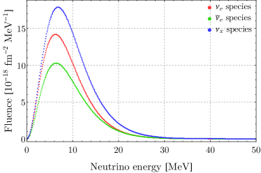
(a)

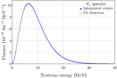
(b)

Figure 1: LABEL:sub@fig:fluenza1 Fluences for the three neutrino species obtained by time integration of equation (3) with the parameters of figure 3 in ref. [19]. LABEL:sub@fig:fluenza2 Comparison, for $\overline{\nu}_{\mathrm{e}}$, of the fluence shown in the left panel and the Garching energy distribution (13) with the effective parameters reported in table 1.

2.2 Flavor transformation of the neutrino fluences

During the neutrino propagation through the star, the neutrino fluences can undergo spectral swappings due to shock waves, turbulence and to the neutrino interactions with the matter composing the astrophysical medium as well as with background neutrinos and antineutrinos. Such interactions are implemented in the mean-field neutrino evolution equations and produce a variety of flavor conversion phenomena [25]. Since the impact of neutrino self-interactions on the neutrino fluxes still need to be fully assessed, here we only consider the fluence modification due to the Mikheyev-Smirnov-Wolfenstein (MSW) effect [26, 27], as done in refs.[7, 8]. We take normal ordering as reference scenario. Therefore, the fluences at detection $F_{\nu_{\mbox{\tiny e}}},F_{\overline{\nu}_{\!\;\!\mbox{\tiny e}}}$ become the following linear combination of the neutrino fluences at the neutrinosphere $F_{\overline{\nu}_{\!\;\!\mbox{\tiny e}}}^{0},F_{\nu_{\mbox{\tiny$x$}}}^{0}$ [22, 28]:

$$\begin{cases}F_{\nu_{\mbox{\tiny e}}}&=F_{\nu_{\mbox{\tiny$x$}}}^{0}\\ F_{\overline{\nu}_{\!\;\!\mbox{\tiny e}}}&=P_{\mathrm{e}}\cdot F_{\overline{\nu}_{\!\;\!\mbox{\tiny e}}}^{0}+(1-P_{\mathrm{e}})\cdot F_{\nu_{\mbox{\tiny$x$}}}^{0},\end{cases}$$ (14)

where $P_{\mathrm{e}}=|U_{e1}|^{2}=|\cos\theta_{12}\cos\theta_{13}|^{2}\approx 0.70$.

3 Likelihood analysis in Hyper-Kamiokande

We study the signal given by a supernova explosion located at a distance of $D=$10\text{\,}\mathrm{kpc}$$, assumed to be known precisely. To give a term of comparison, in the following we will consider also the optimistic situation of a supernova exploding at $D=$2\text{\,}\mathrm{kpc}$$.

We consider Hyper-Kamiokande as reference detector which is expected to have a fiducial mass of $374\text{\,}\mathrm{kton}$ and to be built in the near future [29]. We focus on the two main reactions of neutrino detection in water Cherenkov detectors, namely inverse beta decay (IBD) and elastic scattering onto electrons (ES).

Considering the process $j=\mathrm{IBD}$, ES and the neutrino species $i$, the number of expected events can be expressed as

$$\mathrm{N}_{j}=N_{T}\int_{E_{\mathrm{thr}}}^{\infty}\operatorname{d}\!{E}\,\frac{\operatorname{d}\!{F}_{i}}{\operatorname{d}\!{E}}\,\sigma_{ji},$$ (15)

where $N_{T}$ is the number of targets and $\sigma_{ji}$ is the cross section. The quantity $E_{\mathrm{thr}}$ is the minimum of neutrino energies which depends on the detector threshold assumed to be $5\text{\,}\mathrm{MeV}$ in the following. The detailed expressions of $\sigma_{ji}$ and $E_{\mathrm{thr}}$ as well as for the differential rates of expected events can be found in ref.  [8]. The distributions of events are shown in figure 2.

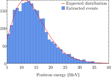
(a)

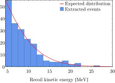
(b)

Figure 2: Energy distribution of the 2437 IBD LABEL:sub@fig:IBDeventi and 198 ES LABEL:sub@fig:ESeventi events. In each figure the histogram of the extracted data is plotted together with the expected distribution.

The total number of expected events with the fluences, described by the true parameters in table 1, is

$$\mathrm{N}_{\mathrm{IBD}}=2566\qquad\mathrm{N}_{\mathrm{ES}}=188.$$ (16)

A real experiment would see a number of events $n_{j}$ given by Poissonian variation of the expected ones. In our case we obtained

$$n_{\mathrm{IBD}}=2437\qquad n_{\mathrm{ES}}=198.$$ (17)

For the $2\text{\,}\mathrm{kpc}$ case we found $\mathrm{N}_{\mathrm{IBD}}=64151$, $\mathrm{N}_{\mathrm{ES}}=4707$, $n_{\mathrm{IBD}}=64278$, $n_{\mathrm{ES}}=4739$.

Following the theoretical distribution, for each event we extract the corresponding neutrino energy supposed to be known with negligible smearing. The results for IBD and ES are shown in figures 2a and 2b respectively and compared with the theoretical expectation.

In order to analyze the IBD and ES extracted events we use a binned likelihood

$$\mathcal{L}_{j}\left(\text{param.}\right)\propto\prod_{i=1}^{N_{\text{bin}}}\frac{\nu_{i}^{n_{i}}}{n_{i}}e^{-\nu_{i}}\quad\text{with}\>j=\text{IBD, ES};$$ (18)

where the number of expected events $\nu_{i}$, for the process $j$, in the $i$-th bin, is compared with the number $n_{i}$ got from the random extraction. In order to be able to get the most from the extracted events, bin widths vary according to the energy. We adopt the same energy bin sizes as in refs. [30, 7, 8].

The analysis begins with the definition of a prior in which the parameters are free to vary (Table 1). The ones for the total energies $\mathcal{E}_{i}$ and mean energies $\langle E_{i}\rangle$ are a little lower than the ones of our previous analyses [7, 8]. This is justified, since we consider the explosion at late times. Moreover, note that for the $\overline{\nu}_{\mathrm{e}}$ and $\nu_{x}$ species the priors are wide enough to fully include the set of accepted points at $3\sigma$ confidence level (see below). This is not true for the $\nu_{\mathrm{e}}$ species; however, its parameters are almost undetermined in this kind of detectors, so a wider prior has no purpose (see e.g. the discussion in [8]).

We emphasize that, given the low number of IBD$+$ES events (17), based on the analysis done for Super-Kamiokande [8] it is clear that the pinching parameters $\alpha_{i}$ will be undetermined for all species. Indeed, the likelihood is not able to constraint their variation in the neighborhood of the true values, but allows them to span almost uniformly up to values that are not of any usefulness. Thus, defining the prior is equivalent to constrain these parameters. Therefore it is of crucial importance how the $\alpha$ prior is defined, since, as we will see, the reconstruction of the emission radii is strictly related to the pinching range.

In the following, we perform three different analysis. The first one, called “default” takes as prior on $\alpha$ the conservative range $\left[2.1,\,3.5\right]$. It is opposed to a scenario in which we make the hypothesis that $\alpha$ is well constrained by supernova simulations. It will be referred to “$\alpha$–prior+” and the range considered is $\alpha\in\left[2.27,\,3.47\right]$. In the third scenario, called simply “$\alpha$–prior”, we assume a mildly-constrained range between $2.1$ and $2.6$. Notice that in our previous works [7, 8] we considered as reasonable interval the range $[1.5,\,3.5]$, suggested in ref. [6] for the time-independent analysis including the whole neutrino time signal. However, $\alpha\to 2$ approaches to a Maxwell-Boltzmann distribution, that means $\eta\to-\infty$ and consequently the loss of consistency of equation (8).

Once the priors are defined (table 1), the Monte Carlo based analysis is performed by extraction of random points inside the $n$-dimensional region. Given a confidence level (CL), each point $P$ is accepted if it satisfies the relation

$$\log\mathcal{L}\left(P\right)\geq\log\mathcal{L}_{max}-\frac{A}{2},\quad\text{with}\quad\int_{0}^{A}\chi^{2}(N_{\mathrm{dof}};z)\,\mathrm{d}{z}=\mathrm{CL};$$ (19)

where $\chi^{2}(N_{\mathrm{dof}};z)$ is a chi-square distribution characterized by $N_{\mathrm{dof}}$ degrees of freedom and $\mathcal{L}_{max}$ is the maximum of the (global) likelihood inside the region. As done and discussed in our previous papers, we assume a $100\%$ tagging efficiency between IBD and ES events. In this manner, the global likelihood is simply the product between the IBD and ES ones.

4 Reconstruction of the proto-neutron star radius $R$

We present here the numerical results of our analysis. Two cases will be considered. In the first one, the proto-neutron star radius is reconstructed based on a three flavor framework and a 9 degrees of freedom likelihood analysis. In the second one we employ one effective neutrino flavor and a three degrees of freedom likelihood analysis. We will not be discussing here the precision with which one can determine the parameters defining the neutrino fluences in eq. (13) — see table 1. Indeed this aspect is investigated in detail in refs. [7, 8] for the full neutrino time signal.

4.1 Impact of the pinching parameter on $R$ reconstruction

4.1.1 Three flavor analysis

Once we find the accepted points according to (19), we can use the corresponding parameters $\left(\mathcal{E}_{i},\,\langle E_{i}\rangle,\,\alpha_{i}\right)$ and reconstruct the radii $R_{i}$ for the three species by using equation (8) and the relation between $\alpha_{i}$ and $\eta_{i}$ (12). This gives us one point in the 12-dimensional region following the parameters distribution.

Projecting these points onto the axes of the multi-dimensional region gives PDF histograms, the flux parameters $\mathcal{E}_{i}$, $\langle E_{i}\rangle$, $\alpha_{i}$ for the three neutrino species. Their mean and standard deviation are reported in table 2 for the default and $\alpha$–prior+ analysis.

			default			$\alpha$–prior+
		True	Mean	SD	%	Mean	SD	%
$\nu_{\mathrm{e}}$	$\mathcal{E}$ [foe]	2.49	5.22	2.7	52.5	5.21	2.7	52.7
			(5.10)	(2.7)	(53.5)	(4.68)	(2.7)	(57.4)
3-9	$\langle E\rangle$ [MeV]	8.81	8.95	2.9	32.0	8.93	2.9	32.0
			(9.15)	(2.7)	(29.0)	(8.7)	(2.5)	(29.0)
3-9	$\alpha$	2.39	2.80	0.40	14.4	2.37	0.06	2.43
			(2.82)	(0.40)	(14.3)	(2.37)	(0.06)	(2.43)
$\overline{\nu}_{\mathrm{e}}$	$\mathcal{E}$ [foe]	1.96	1.66	0.39	23.4	1.71	0.41	23.7
			(2.04)	(0.17)	(8.34)	(2.02)	(0.16)	(8.07)
3-9	$\langle E\rangle$ [MeV]	9.14	9.78	1.2	11.8	9.38	0.82	8.79
			(9.35)	(0.44)	(4.69)	(9.32)	(0.29)	(3.13)
3-9	$\alpha$	2.28	2.78	0.4	14.3	2.37	0.06	2.44
			(2.38)	(0.2)	(8.32)	(2.37)	(0.06)	(2.41)
$\nu_{x}$	$\mathcal{E}$ [foe]	3.62	3.78	0.81	21.3	3.85	0.84	21.8
			(3.43)	(0.38)	(11.)	(3.52)	(0.36)	(10.1)
3-9	$\langle E\rangle$ [MeV]	9.51	9.71	1.1	11.4	9.31	0.8	8.62
			(9.45)	(0.57)	(5.99)	(9.33)	(0.38)	(4.02)
3-9	$\alpha$	2.46	2.77	0.4	14.3	2.37	0.06	2.43
			(2.52)	(0.29)	(11.4)	(2.37)	(0.06)	(2.42)

Table 2: Results of the flux parameter reconstruction in Hyper-Kamiokande, for the three neutrino species, from the time-window $6\div$10\text{\,}\mathrm{s}$$, combining IBD and ES signal. The two blocks named “default” and “$\alpha$–prior+” refer to an $\alpha$ prior of $[2.1,\,3.5]$ and $[2.27,\,2.47]$ respectively. The top rows present the $D=$10\text{\,}\mathrm{kpc}$$ analysis, while the quantities in parentheses are the result of a $D=$2\text{\,}\mathrm{kpc}$$ explosion. For each parameter we give its true value, the mean of the parameter distribution, its standard deviation (SD) and the overall accuracy.

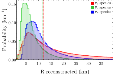
(a)

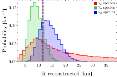
(b)

Figure 3: Distribution of the reconstructed proto-neutron star radii for the three neutrino species. The left panel LABEL:sub@fig:HR3a0 shows the results obtained with the most conservative prior, while the right panel LABEL:sub@fig:HR3a1 presents the ones for a well defined pinching parameter (see text). The dashed vertical lines show the true values for the radii. Notice that the radius tail for the $\nu_{\mathrm{e}}$ species extends up to $214\text{\,}\mathrm{km}$ and $130\text{\,}\mathrm{km}$ in figure LABEL:sub@fig:HR3a0 and LABEL:sub@fig:HR3a1 respectively.

Looking at the $10\text{\,}\mathrm{kpc}$ case in table 2, the total energy $\mathcal{E}_{\overline{\nu}_{\!\;\!\mbox{\tiny e}}}$ and the mean energy $\langle E_{\overline{\nu}_{\!\;\!\mbox{\tiny e}}}\rangle$ are reconstructed with an accuracy of $\sim 23\%$ and $\sim 12\%$. The situation does not improve much even considering the very aggressive scenario “$\alpha$–prior+”. The knowledge of the $\nu_{x}$ reaches an accuracy on $\mathcal{E}_{\nu_{\mbox{\tiny$x$}}}$ and $\langle E_{\nu_{\mbox{\tiny$x$}}}\rangle$ of $\sim 21\%$ and $\sim 11\%$ respectively. Except for the pinching, the accuracy in the reconstruction of the total and average energies for $\overline{\nu}_{\mathrm{e}}$ and $\nu_{x}$ improves for the $2\text{\,}\mathrm{kpc}$ case.

The pinching parameters $\alpha_{i}$ are reconstructed with almost the same accuracies among species, namely $\sim 14\%$ and $\sim 2.4\%$ for the “default”and “$\alpha$–prior+” analyses respectively. In the latter case the accuracy obviously improves but only because the prior is tighter. Indeed, the listed standard deviations are similar to the ones expected for a flat distribution inside the range of the prior, namely $0.40$ for $\alpha\in\left[2.1,\,3.5\right]$, $0.14$ for $\alpha\in\left[2.1,\,2.6\right]$ and $0.06$ for $\alpha\in\left[2.27,\,2.47\right]$. This is the same reason of the “better” reconstruction of the $\nu_{\mathrm{e}}$ species: it is just a matter of prior, being the flux properties of this species almost undetermined.

The neutrino signal in Super-Kamiokande and Hyper-Kamiokande have been already analyzed in [8]. It is worthwhile to compare these cases with the signal in the time window $6\div$10\text{\,}\mathrm{s}$$. The number of detected events in Hyper-Kamiokande in the window $6\div$10\text{\,}\mathrm{s}$$ is similar to the number of events seen for the whole explosion in Super-Kamiokande at the same distance. The total number of expected events in Hyper-kamiokande, in the late-time window, for an explosion at $D=$2\text{\,}\mathrm{kpc}$$ is comparable with the total number of events it would see at $D=$10\text{\,}\mathrm{kpc}$$. Therefore, one might naively expect to reconstruct the quantities $\mathcal{E}_{i}$ and $\langle E_{i}\rangle$ with the same accuracies discussed in ref. [8] for the whole signal in Super-Kamiokande and Hyper-Kamiokande at $D=$10\text{\,}\mathrm{kpc}$$. However, this is not the case. In particular, concerning the $\overline{\nu}_{\mathrm{e}}$ species, the reconstruction of the total energy $\mathcal{E}_{\overline{\nu}_{\!\;\!\mbox{\tiny e}}}$ and the mean energy $\langle E_{\overline{\nu}_{\!\;\!\mbox{\tiny e}}}\rangle$ worsens by a factor of 2. These features are not due to the likelihoods or the particular analyses: redoing the calculations using a likelihood with smaller bins lead to the same results. A possible explanation of this behavior may lie in the different values of the distributions. Indeed, the total emitted energies $\mathcal{E}_{i}$ and mean energies $\langle E_{i}\rangle$ of the late time emission are significantly lower than the ones in the whole time window [8].

In all the analyses, the most significant contribution to the statistics is given by the IBD events. As already underlined in [30], if the spectral shape (pinching) is unknown, the oscillation mechanism introduces a degeneracy in the fluxes, especially if the IBD signal only is considered. It has been shown in [7] that the combination of inverse beta decay and elastic scattering can break the degeneracy between the total and the mean energies. However, it is reasonable to expect this works better when the contamination of $\nu_{x}$ is smaller. Among the $2566$ expected IBD events at $10\text{\,}\mathrm{kpc}$ (16), $1393$ are due to the emitted $\overline{\nu}_{\mathrm{e}}$ and $1173$ to the emitted $\nu_{x}$, i.e. $54\%$ and $46\%$ respectively. With the true parameters assumed in our previous papers [7, 8] these percentage were $63\%$ and $37\%$. This suggest the previous analyses gave better results because the two flux components were “less entangled”. However, such a combination had not helped to get a good identification of the second moment of the fluence distribution, as shown in ref. [8].

These uncertainties propagate to $R_{i}$ reconstruction. The histograms describing the radii distributions given in the default and $\alpha$–prior+ analysis are shown in figure 3a and 3b respectively, while the numerical values are listed in table 3. As expected, in both cases $R_{\nu_{\mbox{\tiny e}}}$ is undetermined, since the flux parameters for this neutrino species remain unknown. Concerning $R_{\overline{\nu}_{\!\;\!\mbox{\tiny e}}}$ and $R_{\nu_{\mbox{\tiny$x$}}}$, the accuracy remains poor, being around $50\%$ in the conservative range $\alpha\in\left[2.1,\,3.5\right]$ and $25\%$ with the tightest prior $\alpha\in\left[2.27,\,2.47\right]$ at $3\sigma$ (CL).

		default			$\alpha$–prior			$\alpha$–prior+
	true	Mean	SD	Acc	Mean	SD	Acc	Mean	SD	Acc
	$[$\mathrm{km}$]$	$[$\mathrm{km}$]$	$[$\mathrm{km}$]$	$[\%]$	$[$\mathrm{km}$]$	$[$\mathrm{km}$]$	$[\%]$	$[$\mathrm{km}$]$	$[$\mathrm{km}$]$	$[\%]$
$\nu_{\mathrm{e}}$	11.9	18.9	18.6	98.0	26.4	24.1	91.3	23.8	20.5	86.1
		(16.8)	(16.2)	(96.5)	(24.4)	(21.1)	(86.4)	(22.2)	(17.9)	(80.8)
$\overline{\nu}_{\mathrm{e}}$	11.5	7.1	4.0	56.0	10.1	3.9	38.4	9.2	2.4	25.6
		(10.9)	(3.8)	(34.4)	(10.8)	(3.1)	(28.7)	(9.9)	(1.2)	(12.2)
$\nu_{x}$	11.4	10.8	5.9	54.6	15.4	5.8	37.4	13.9	3.4	24.5
		(12.3)	(4.9)	(40.0)	(14.1)	(4.2)	(29.8)	(13.0)	(1.8)	(13.7)

Table 3: Results of the radii reconstruction in Hyper-Kamiokande, for the three neutrino species, from the time-window $6\div$10\text{\,}\mathrm{s}$$, combining IBD and ES signal. The three blocks named “default”, “$\alpha$–prior” and “$\alpha$–prior+” refer to an $\alpha$ prior of $[2.1,\,3.5]$, $[2.1,\,2.6]$, and $[2.27,\,2.47]$ respectively. The top rows present the $D=$10\text{\,}\mathrm{kpc}$$ analysis, while the quantities in parentheses are the result of a $D=$2\text{\,}\mathrm{kpc}$$ explosion. For each radius we give its true value, the mean of the parameter distribution, its standard deviation (SD) and the overall accuracy.

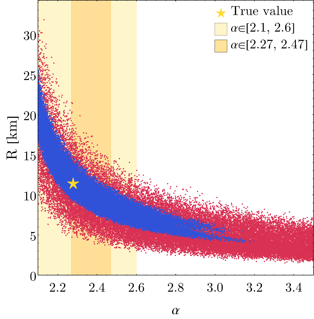
(a)

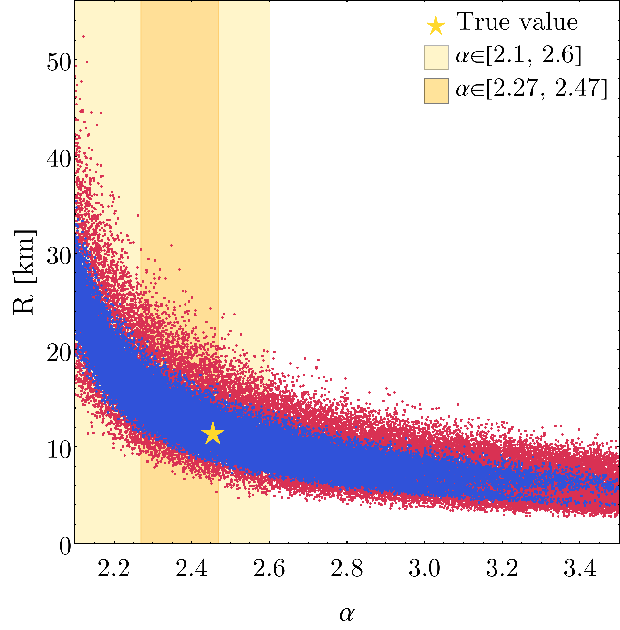
(b)

Figure 4: Projection onto the $\alpha$–$R$ plane of 40k points, in the $D=$10\text{\,}\mathrm{kpc}$$ (red) and $D=$2\text{\,}\mathrm{kpc}$$ (blue) analysis, for the $\overline{\nu}_{\mathrm{e}}$ LABEL:sub@fig:S3s2 and $\nu_{x}$ LABEL:sub@fig:S3s3 species. In both panels, the star marks the true values, while the bands highlight the different assumptions on the prior of $\alpha$.

The explanation of this results can be found projecting the extracted points onto two-dimensional planes, as shown in figure 4 for the $\alpha$–$R$ plane and for the $\overline{\nu}_{\mathrm{e}}$ and $\overline{\nu}_{x}$ species. From these plots, one can clearly see a strong correlation between $\alpha$ and $R$. This correlation does not improve from the $D=$10\text{\,}\mathrm{kpc}$$ to the $D=$2\text{\,}\mathrm{kpc}$$ analysis, so it is not due to the statistics. Indeed, it is somehow expected. As we already discussed, the pinching parameters are almost undetermined. The information about their values, however, is crucial in the radii reconstruction — see equation (8). Indeed, figure 4 shows a tight correlation that cannot be resolved with neutrinos alone.

Moreover, notice that our “true radii” are computed from equations (8, 12) by taking the true values $\left(\mathcal{E}_{i}^{*},\,\langle E_{i}^{*}\rangle,\,\alpha_{i}^{*}\right)$ given in table 1. The result is reported in the first column of table 3. We would like to underline that the values obtained in this way are in principle different from the radii computed in other ways, e.g. by the temporal mean of the $R_{i}$ provided by the simulation of ref. [19] and defined as the region in which the neutrino opacity reaches the value of $2/3$. The latter are

$$R_{\nu_{\mbox{\tiny e}}}=$12.69\text{\,}\mathrm{km}$,\quad R_{\overline{\nu}_{\!\;\!\mbox{\tiny e}}}=$12.19\text{\,}\mathrm{km}$,\quad R_{\nu_{\mbox{\tiny$x$}}}=$12.09\text{\,}\mathrm{km}$.$$ (20)

As one can see comparing table 2 and equation (20), the latter are about $6\div 7\%$ bigger.

We remind that the radii reconstructed by the neutrino data analyses are neutrinosphere radii, that, according to [19] are underneath the proto-neutron star radii in which we are interested, while the two radii are the same within $10\%$ [4, 19]. In view of the importance of this connection, a systematic work on simulations is necessary, to quantify accurately the comparison. When drawing conclusions on the precision achieved for the proton-neutron star radii, the entailed systematic errors should be taken into account.

4.1.2 One effective flavor analysis

		default			$\alpha$–prior+
	True	Mean	SD	Acc	Mean	SD	Acc
$\mathchoice{\widetilde{\mathcal{E}}}{\tilde{\mathcal{E}}}{\tilde{\mathcal{E}}}{\tilde{\mathcal{E}}}$ [foe]	2.47	2.31	0.11	4.6	2.33	0.1	4.41
$\langle\mathchoice{\widetilde{E}}{\tilde{E}}{\tilde{E}}{\tilde{E}}\rangle$ [MeV]	9.31	9.53	0.33	3.46	9.38	0.18	1.88
$\mathchoice{\widetilde{\alpha}}{\tilde{\alpha}}{\tilde{\alpha}}{\tilde{\alpha}}$	2.35	2.51	0.26	10.3	2.37	0.058	2.43
$\mathchoice{\widetilde{R}}{\tilde{R}}{\tilde{R}}{\tilde{R}}$ [km]	11.1	9.9	3.8	38.3	10.5	1.1	10.6

Table 4: Results at $3\sigma$ CL as provided by the analysis on the IBD signal fitted with only one effective flavor $\mathchoice{\widetilde{\nu}}{\tilde{\nu}}{\tilde{\nu}}{\tilde{\nu}}$. The two blocks named “default” and “$\alpha$–prior+” refer to an $\alpha$ prior of $[2.1,\,3.5]$, and $[2.27,\,2.47]$ respectively. For each parameter we listed the true value, mean, standard deviation (SD) and accuracy.

One way to approach the issue of the proto-neutron star radius reconstruction is to perform an analysis based on one effective flavor $\mathchoice{\widetilde{\nu}}{\tilde{\nu}}{\tilde{\nu}}{\tilde{\nu}}$, instead of three flavors. In this case, the expected IBD flux in figure 2a can be fitted assuming a Garching function depending upon three parameters only, whose true values are

$$\mathchoice{\widetilde{\mathcal{E}}}{\tilde{\mathcal{E}}}{\tilde{\mathcal{E}}}{\tilde{\mathcal{E}}}^{*}=$2.4727\text{\,}\mathrm{foe}$;\quad\langle\mathchoice{\widetilde{E^{*}}}{\tilde{E^{*}}}{\tilde{E^{*}}}{\tilde{E^{*}}}\rangle=$9.3065\text{\,}\mathrm{MeV}$;\quad\mathchoice{\widetilde{\alpha}}{\tilde{\alpha}}{\tilde{\alpha}}{\tilde{\alpha}}^{*}=2.35023;\quad\mathchoice{\widetilde{R}}{\tilde{R}}{\tilde{R}}{\tilde{R}}^{*}=$11.122\text{\,}\mathrm{km}$;$$ (21)

where the true radius has been obtained by equation (8). Then, the flux can be studied as it were composed by one non-oscillating effective species $\mathchoice{\widetilde{\nu}}{\tilde{\nu}}{\tilde{\nu}}{\tilde{\nu}}$. Again, we perform three different analyses, taking the priors on $\mathchoice{\widetilde{\alpha}}{\tilde{\alpha}}{\tilde{\alpha}}{\tilde{\alpha}}$ listed in table 1 and restricting ourselves to the $D=$10\text{\,}\mathrm{kpc}$$ case.

For completeness, the results are shown in table 4. As one can see, the normalization $\mathchoice{\widetilde{\mathcal{E}}}{\tilde{\mathcal{E}}}{\tilde{\mathcal{E}}}{\tilde{\mathcal{E}}}$ and the mean $\langle\mathchoice{\widetilde{E}}{\tilde{E}}{\tilde{E}}{\tilde{E}}\rangle$ of the distribution are measured with great accuracy, namely $\sim 4\%$ and $\sim 3\%$ in the less constrained analysis. This precision does not improve much with the most restrictive $\mathchoice{\widetilde{\alpha}}{\tilde{\alpha}}{\tilde{\alpha}}{\tilde{\alpha}}$ prior. On the other hand, the spectral shape is not known at all, with a distribution of the pinching almost flat in the prior. This of course propagates to the radius. Figure 5a shows the projection onto the $\mathchoice{\widetilde{\alpha}}{\tilde{\alpha}}{\tilde{\alpha}}{\tilde{\alpha}}$–$\mathchoice{\widetilde{R}}{\tilde{R}}{\tilde{R}}{\tilde{R}}$ plane of 40k accepted points at $3\sigma$ CL. Figure 5b reports the distribution of the reconstructed radius, assuming different priors on $\mathchoice{\widetilde{\alpha}}{\tilde{\alpha}}{\tilde{\alpha}}{\tilde{\alpha}}$. As one can see, the parameter region is thinner with respect to figure 4, but the correlation is still present. This means that, in the most conservative case, the emission radius is determined within $\sim 40\%$; while it can be reduced up to $10\%$, but with an aggressive prior.

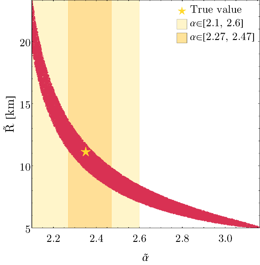
(a)

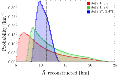
(b)

Figure 5: Panel LABEL:sub@fig:Sc1s shows the projection of 40k accepted points at $3\sigma$ CL onto the $\mathchoice{\widetilde{\alpha}}{\tilde{\alpha}}{\tilde{\alpha}}{\tilde{\alpha}}$–$\mathchoice{\widetilde{R}}{\tilde{R}}{\tilde{R}}{\tilde{R}}$ plane. The star marks the true values, while the bands highlight the different assumptions on the prior of $\alpha$. Panel LABEL:sub@fig:HR1s shows the distributions of the reconstructed radii in the three different analyses, characterized by a different prior of $\alpha$. The dashed line marks the true value.

		$R$–prior			$R$–prior+
	true	Mean	SD	Acc	Mean	SD	Acc
$\nu_{\mathrm{e}}$	2.39	2.79	0.39	14.1	2.78	0.39	14.0
		(2.83)	(0.37)	(13.1)	(2.83)	(0.37)	(13.1)
$\overline{\nu}_{\mathrm{e}}$	2.28	2.33	0.16	6.73	2.27	0.1	0.55
		(2.33)	(0.11)	(4.81)	(2.29)	(0.053)	(2.3)
$\nu_{x}$	2.46	2.58	0.27	10.3	2.5	0.19	7.45
		(2.51)	(0.17)	(6.96)	(2.45)	(0.09)	(3.67)

Table 5: Results of the $\alpha$ parameter reconstruction in Hyper-Kamiokande, for the three neutrino species, from the time-window $6\div$10\text{\,}\mathrm{s}$$, combining IBD and ES signal. The analysis has been performed with the default $\alpha$ prior, keeping only the points whose radii are inside the radius prior. The two blocks named “$R$–prior” and “$R$–prior+” refer to a $R$ prior of $[8,\,16]$ $\mathrm{km}$ and $[10.2,\,13.1]$ $\mathrm{km}$ respectively. The top rows present the $D=$10\text{\,}\mathrm{kpc}$$ analysis, while the quantities in parentheses are the result of a $D=$2\text{\,}\mathrm{kpc}$$ explosion. For each $\alpha_{i}$ we give its true value, the mean of the parameter distribution, its standard deviation (SD) and the overall accuracy.

Neutron star masses and radii depend on the neutron star equation of state and also could be modified in extended theories of gravity. Future measurements with X-rays and gravitational waves will obtain tight constraints on the mass and radius relation of cold neutron stars and on the radius itself. Gravitational waves observations might discover extended theories of gravity. With all the caveats of the present analysis, we would like to show the sensitivity of the gravitational binding energy of the nascent neutron star to theories beyond general relativity such as the so-called $f(R)$ theories [31]. Figure 6 shows the gravitational mass, the baryonic mass as well as the gravitational binding energy as a function of the neutron star radius. Results are shown both for general relativity as well as for $f(R)=R+\alpha R^{2}$ extended theory of gravity for three different values of $\alpha$ (see appendix A.2 for the corresponding equations). While masses and radii differ significantly from the general relativity predictions for large $\alpha$ values as expected, the gravitational binding energy turns out to have much smaller sensitivity to such extended theories of gravity even for $\alpha$ as large as 20. The results are plotted for two different equations of state, i.e. APR and Sly [32].

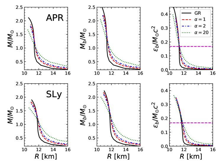
Figure 6: Predictions for macroscopic properties of a neutron star, for the two equations of state APR (upper) and SLy (lower figures). The quantities on the $y$-axis — neutron star mass (left), baryonic mass (middle) and gravitational binding energy (right figures) — are plotted as a function of the neutron star radius. $M_{\odot}$ is the Sun mass. The results correspond either to predictions in general relativity (GR) or for $f(R)$ theories with $f(R)=R+\alpha R^{2}$ and three different $\alpha$ values (see text). To guide the eye, we plot the value $3\text{\times}{10}^{53}\text{\,}\mathrm{erg}$ (the magenta dashed lines) in the third panels.

4.2 Inverting the perspective: constraining the effective pinching

Our results show that the reconstructed radii vary significantly with $\alpha$. Conversely, assuming a prior knowledge on the radius could help in the determination of the pinching parameter $\alpha$. Indeed, we can take the extracted points in the IBD$+$ES three flavor analysis (with broad $\alpha$) and analyze only those whose radii are inside a defined physical prior. Current neutron star equations of state, compatible with neutron star observations, predict $R\in[8,16]$ $\mathrm{km}$. This is our first prior for the neutrinosphere, called “$R$–prior”. On the other hand, we can also assume an aggressive prior about the radius knowledge, i.e. $R\in[10.2,13.1]$ $\mathrm{km}$ which could result from independent measurements. It will be called “$R$–prior+”. The results for the pinching reconstruction for the two priors are given in table 5.

Thanks to the correlation between $\alpha$ and $R$, under the $R$–prior case, an accuracy of $7\%$ and $10\%$ can be achieved on the pinching parameters of $\overline{\nu}_{\mathrm{e}}$ and $\nu_{x}$ respectively (for a supernova at $10\text{\,}\mathrm{kpc}$). With the more aggressive $R$–prior+, the accuracy improves to $\sim 1\%$ and $\sim 7\%$ for the $\overline{\nu}_{\mathrm{e}}$ and $\nu_{x}$ species respectively. As expected, the determination of $\alpha$ for the $\nu_{\mathrm{e}}$ species does not improve.

Concerning the other flux parameters, the accuracy of the reconstructed values is very similar for both priors: the accuracy on the emitted energies for $\overline{\nu}_{\mathrm{e}}$ and $\nu_{x}$ species is $\sim 20\%$; the accuracy on their mean energies is $\sim 7\div 8\%$. These values are similar to the ones reported in ref. [8] for Super-Kamiokande, although we remark that the emitted energy $\mathcal{E}_{\overline{\nu}_{\!\;\!\mbox{\tiny e}}}$ was there determined with an accuracy of $\sim 10\%$.

5 Conclusions

We have explored the possibility to reconstruct the radius of the newly formed neutron star in a core-collapse supernova explosion through its neutrino time signal. To this aim, we have performed a nine-degrees of freedom likelihood analyses, considering the total energy, the average energy and the pinching parameter for the three neutrino species. These characterize th $\nu_{e}$, $\overline{\nu}_{\mathrm{e}}$ and $\nu_{x}$ fluences which are assumed to be black-body spectra equipped with pinching to account for the deviations from thermal distributions. The neutrino time signal is adopted from simulations by Roberts and Reddy. The interval of time chosen for the analysis, between 6 and 10 seconds, is motivated by the fact that the neutron star and neutrinosphere radii are approximatively time independent over this range which justifies the use of fluences, instead of the time-dependent neutrino signal [19].

We have combined inverse beta decay and elastic scattering in a water Cherenkov detector of the size of the future Hyper-Kamiokande, assuming ideal detector performance — namely, an efficiency approaching $100\%$. The numerical results have unravelled a tight correlation between the pinching parameters and the reconstructed neutron star radius. We performed three analysis, ranging from a very conservative to a rather aggressive one with respect to the prior choices of the pinching parameter. In the most conservative one, the neutrinosphere radius could be determined only with a precision of $35\%$ ($56\%$) for a supernova at $2\text{\,}\mathrm{kpc}$ ($10\text{\,}\mathrm{kpc}$) for $\overline{\nu}_{\mathrm{e}}$; whereas with the most aggressive prior the precision could improve to $12\%$ ($26\%$) for a supernova at $2\text{\,}\mathrm{kpc}$ ($10\text{\,}\mathrm{kpc}$). A similar accuracy is obtained for $\nu_{x}$. While these results might be sufficient to probe (exclude) the cases of oscillations into mirror [12] or pseudo-Dirac neutrinos [13], they indicate the difficulty in determining the neutron star radius precisely through neutrino measurements. This conclusion is not altered if statistics is increased since both the $10\text{\,}\mathrm{kpc}$ and the $2\text{\,}\mathrm{kpc}$ supernova results show similar quantitative trends. Our work indicates the importance of getting precise knowledge on the width of the quasi-thermal neutrino distribution from core-collapse supernova simulations.

One should consider that the neutrino time signal is directly related to the neutrinosphere radii and is a unique observable to get information about them. In order to successfully perform the type of analysis described here, and to interpret the results in connection with the neutron star radius, a systematic study will be required to quantitatively connect the neutrinosphere radii to the radius of the neutron star formed during the explosion which are thought to be within $10\div 15\%$ of each other for the time interval of interest.

By inverting the perspective, we have performed two more analyses: a) implementing in the likelihoods that the neutron star radius (and consequently the radius of the neutrinosphere) varies in the range $8\div$10\text{\,}\mathrm{km}$$; b) assuming that future measurements will narrow its current uncertainty down to $10\%$. In case a) the pinching parameters of the neutrino fluences can be determined with an accuracy of $5\%$ ($7\%$) at $2\text{\,}\mathrm{kpc}$ ($10\text{\,}\mathrm{kpc}$) for $\overline{\nu}_{\mathrm{e}}$ and $7\%$ ($10\%$) at $2\text{\,}\mathrm{kpc}$ ($10\text{\,}\mathrm{kpc}$) for $\nu_{x}$. In case b) the pinching parameters of the neutrino fluences can be determined with an accuracy of $1\%$ ($2\%$) at $2\text{\,}\mathrm{kpc}$ ($10\text{\,}\mathrm{kpc}$) for $\overline{\nu}_{\mathrm{e}}$ and $4\%$ ($7\%$) at $2\text{\,}\mathrm{kpc}$ ($10\text{\,}\mathrm{kpc}$) for $\nu_{x}$. The other parameters of the fluences can be determined with good precision as well. Likewise, for $\nu_{\mathrm{e}}$ the reconstruction of the corresponding pinching is approximately with a precision of $14\%$ while the determination of the fluence would require the inclusion of $\nu_{\mathrm{e}}$ sensitive detection channels.

Appendix A Tolman-Oppenheimer-Volkoff equations

In order to obtain the mass-radius relation for neutron stars we have solved the Tolman-Oppenheimer-Volkoff (TOV) equations which govern the physics of the matter-geometry in spherically symmetric space-time [33]. We have considered both general theory of relativity and extended theories of gravity, in particular the so-called $f(R)$ theories. We also comment on how to deal with the problem numerically so that the interested reader could reproduce the plots in figure 3.

A.1 General relativity case

The geometry of a spherically symmetric space-time could be described by the metric specified by

$$\operatorname{d}\!{s}^{2}=e^{2w}c^{2}\operatorname{d}\!{t}^{2}-e^{2\lambda}\operatorname{d}\!{r}^{2}-r^{2}(\operatorname{d}\!{\theta}^{2}+\sin^{2}\theta\operatorname{d}\!{\phi}^{2}),$$ (22)

where $r$ denotes the radial variable and $w(r)$ and $\lambda(r)$ are functions of $r$. From the Einstein’s equation one can derive the TOV equations in which the three degrees of freedom $p$, $\lambda$ and $w$ are then governed by

$$\frac{\operatorname{d}\!{p}}{\operatorname{d}\!{r}} =-(\rho c^{2}+p)\frac{\operatorname{d}\!{w}}{\operatorname{d}\!{r}},$$ (23)

$$\frac{\operatorname{d}\!{\lambda}}{\operatorname{d}\!{r}} =\frac{4\pi rG\rho}{c^{2}}e^{2\lambda}-\frac{e^{2}\lambda}{2r}+\frac{1}{2r},$$ (24)

and

$$\frac{\operatorname{d}\!{w}}{\operatorname{d}\!{r}}=\frac{4\pi rGp}{c^{4}}e^{2\lambda}+\frac{e^{2}\lambda}{2r}-\frac{1}{2r},$$ (25)

where $G$ is the constant of gravity and the energy density $\rho$, in principle, is related to the pressure $p$ through the equation of state (EOS).

To solve the TOV equations in GR numerically, one should note that the TOV equations for $p$ and $\lambda$ could be written in a form which is explicitly decoupled from $w$. This means that to integrate them, it is only required to provide two initial values. One for $\lambda$ and one for $p$, namely $p(r=0)=p(\rho_{c})$ and $\lambda(r=0)=0$ with $\rho_{c}$ being the value of the energy density at the center of the neutron star.

A.2 TOV equations in $f(R)$ gravity

In modified theories of gravity, the equation relating the matter to the geometry could be different from the Einstein equation. In particular, in $f(R)$ theory of gravity (in the metric formalism), it could be written as [31]

$$\frac{\operatorname{d}\!{f}(R)}{\operatorname{d}\!{R}}R_{\mu\nu}-\frac{1}{2}f(R)g_{\mu\nu}-\left[\nabla_{\mu}\nabla_{\nu}-g_{\mu\nu}\Box\right]\frac{\operatorname{d}\!{f}(R)}{\operatorname{d}\!{R}}=\frac{8\pi G}{c^{4}}T_{\mu\nu},$$ (26)

where $R$ is the Ricci scalar and $T_{\mu\nu}$ is the energy momentum tensor. In spherically symmetric space time, one can find the generalized TOV equations in $f(R)$ gravity as

$$\frac{\operatorname{d}\!{p}}{\operatorname{d}\!{r}} =-(\rho c^{2}+p)\frac{\operatorname{d}\!{w}}{\operatorname{d}\!{r}},$$ (27)

$$\frac{\operatorname{d}\!{\lambda}}{\operatorname{d}\!{r}} =\frac{8\pi rG\rho e^{2\lambda}}{c^{2}(2f^{\prime}_{R}+rR^{\prime}f^{\prime\prime}_{R})}+\frac{e^{2\lambda}[(r^{2}R-2)f^{\prime}_{R}-fr^{2}]}{2r(2f^{\prime}_{R}+rR^{\prime}f^{\prime\prime}_{R})}+\frac{f^{\prime}_{R}+r[f^{\prime\prime}_{R}(2R^{\prime}+rR^{\prime\prime})+rR^{\prime 2}f^{\prime\prime\prime}_{R}]}{r(2f^{\prime}_{R}+rR^{\prime}f^{\prime\prime}_{R})}$$ (28)

and

$$\frac{\operatorname{d}\!{w}}{\operatorname{d}\!{r}}=\frac{8\pi rGpe^{2\lambda}}{c^{4}(2f^{\prime}_{R}+rR^{\prime}f^{\prime\prime}_{R})}+\frac{e^{2\lambda}[fr^{2}+(2-r^{2}R)f^{\prime}_{R}]-2(f^{\prime}_{R}+2rR^{\prime}f^{\prime\prime}_{R})}{2r(2f^{\prime}_{R}+rR^{\prime}f^{\prime\prime}_{R})},$$ (29)

where the prime ^′ denotes the derivative with respect to $r$ while $f^{\prime}_{R}$, $f^{\prime\prime}_{R}$ and $f^{\prime\prime\prime}_{R}$ are the first, second and third order derivatives of $f(R)$ with respect to $R$. Unlike the case of GR where $R$ is determined statically and explicitly in terms of $\rho$ and $p$

$$R=\frac{8\pi G}{c^{4}}(\rho c^{2}-3p),$$ (30)

in modified gravity, the Ricci scalar could be completely dynamic which adds to the complexity of solving the TOV equations in these theories. In particular, in $f(R)$ gravity one has

$$\frac{\mathop{}\!\mathrm{d^{2}}R}{\operatorname{d}\!{r}^{2}}=\frac{1}{3f^{\prime\prime}_{R}}\left\{-\frac{3f^{\prime\prime}_{R}R^{\prime}}{r}(rw^{\prime}-r\lambda^{\prime}+2)-3f^{\prime\prime\prime}_{R}R^{\prime 2}+e^{2\lambda}(Rf^{\prime}_{R}-2f)+\frac{8\pi Ge^{2\lambda}}{c^{4}}(\rho c^{2}-3p)\right\}.$$ (31)

The generalized TOV equations can be derived for $f(R)=R+\alpha R^{2}$ gravity as

$$\frac{\operatorname{d}\!{p}}{\operatorname{d}\!{r}} =-(\rho c^{2}+p)\frac{\operatorname{d}\!{w}}{\operatorname{d}\!{r}},$$ (32)

$$\frac{\operatorname{d}\!{\lambda}}{\operatorname{d}\!{r}} =\frac{4\pi rG\rho e^{2\lambda}}{c^{2}(1+2\alpha R+\alpha rR^{\prime})}+\frac{e^{2\lambda}(\alpha r^{2}R^{2}-4\alpha R-2)+2+4\alpha r^{2}R^{\prime\prime}+8\alpha rR^{\prime}+4\alpha R}{4r+8\alpha r+4\alpha r^{2}R^{\prime}},$$ (33)

$$\frac{\operatorname{d}\!{w}}{\operatorname{d}\!{r}} =\frac{4\pi rGpe^{2\lambda}}{c^{4}(1+2\alpha R+\alpha rR^{\prime})}+\frac{e^{2\lambda}(-\alpha r^{2}R^{2}+4\alpha R+2)-2-4\alpha R-8\alpha rR^{\prime}}{4r+8\alpha rR+4\alpha r^{2}R^{\prime}},$$ (34)

and

$$\frac{\mathop{}\!\mathrm{d^{2}}R}{\operatorname{d}\!{r}^{2}}=\frac{1}{6c^{4}r\alpha}\left\{e^{2\lambda}(8\pi rG(\rho c^{2}-3p)-c^{4}rR)-6c^{4}\alpha R^{\prime}(2+rw^{\prime}-r\lambda^{\prime})\right\}.$$ (35)

It should be noted that to avoid the ghost instabilities, one could only opt for negative values of $\alpha$, i.e. $\alpha<0$ [34].

Given TOV equations in $f(R)$ gravity, one can integrate them numerically. Here, there are four coupled differential equations for $p$, $\lambda$, $w$ and $R$ which are required to be solved simultaneously. Moreover, one should note that the differential equation for $R$ is second order. To solve these equations numerically, one should know the initial (central) values of $p$, $\lambda$, $w$, $R$ and $R^{\prime}$. The natural choices could be $p(r=0)=p(\rho_{c})$, $\lambda(r=0)=0$ and $R^{\prime}(r=0)=0$. Moreover, the generalized TOV equations are linear in $w$ as in GR and one does not need to know the central value of $w$ beforehand. What should be done is just to take an initial value for $w_{c}$ and then correct it after solving the equations so that it matches the correct boundary value at infinity. However, there is still a big difference between $f(R)$ theories and GR in dealing with TOV equations numerically. In the case of $f(R)$ gravity, one does not know beforehand the value of $R_{c}=R(r=0)$ which is needed to integrate the TOV equations. To overcome this difficulty, the strategy we chose was that we solved the TOV equations by using the bisection method for the range $R_{c}=R_{GR}/10$ to $R_{c}=10R_{GR}$. It turns out that (at least for $R^{2}$ gravity) the value of $R_{c}$ which could result in a physical behavior for $\lambda$ and $R$ is very specific and only for a very narrow range of $R_{c}$ we observed the physically expected asymptotic behavior for this quantities. For other values of $R_{c}$, for example, $\lambda$ could grow/drop monotonously when $r\rightarrow\infty$ instead of the expected asymptotic behavior $\lambda\rightarrow 0$.

References

- [1] H. A. Bethe and J. R. Wilson, Astrophys. J. 295 (1985) 14.
- [2] I. Tamborra, F. Hanke, B. Müller, H. T. Janka and G. Raffelt, Phys. Rev. Lett. 111, no. 12, 121104 (2013) [arXiv:1307.7936 [astro-ph.SR]].
- [3] S. A. Colgate and R. H. White, Astrophys. J. 143, 626 (1966).
- [4] T. J. Loredo and D. Q. Lamb, Phys. Rev. D 65, 063002 (2002) [astro-ph/0107260].
- [5] G. Pagliaroli, F. Vissani, M. L. Costantini and A. Ianni, Astropart. Phys. 31, 163 (2009) [arXiv:0810.0466 [astro-ph]].
- [6] F. Vissani, J. Phys. G 42, 013001 (2015) [arXiv:1409.4710].
- [7] A. Gallo Rosso, F. Vissani and M. C. Volpe, JCAP 1711 (2017) no.11, 036 [arXiv:1708.00760 [hep-ph]].
- [8] A. Gallo Rosso, F. Vissani and M. C. Volpe, JCAP 1804 (2018) no.04, 040 [arXiv:1712.05584 [hep-ph]].
- [9] M. Kobayashi and C. S. Lim, Phys. Rev. D 64, 013003 (2001).
- [10] K. R. Balaji, A. Kalliomaki and J. Maalampi, Phys. Lett. B 524, 153 (2002).
- [11] Z. Berezhiani, D. Comelli and F. L. Villante, Phys. Lett. B 503, 362 (2001)
- [12] V. Berezinsky, M. Narayan and F. Vissani, Nucl. Phys. B 658, 254 (2003)
- [13] J. F. Beacom, N. F. Bell, D. Hooper, J. G. Learned, S. Pakvasa and T. J. Weiler, Phys. Rev. Lett. 92, 011101 (2004)
- [14] F. Vissani and A. Boeltzig, PoS NEUTEL 2015, 008 (2015).
- [15] J. M. Lattimer and A. W. Steiner, Astrophys. J. 784, 123 (2014) [arXiv:1305.3242 [astro-ph.HE]].
- [16] K. Gendreau, and Z. Arzoumanian, Nature Astronomy, 1 (2017), 895; https://heasarc.gsfc.nasa.gov/docs/nicer/index.html.
- [17] J. M. Lattimer and M. Prakash, Phys. Rept. 442, 109 (2007) [astro-ph/0612440].
- [18] B. P. Abbott et al. [LIGO Scientific and Virgo Collaborations], arXiv:1805.11581 [gr-qc].
- [19] L. F. Roberts and S. Reddy, arXiv:1612.03860 [astro-ph.HE].
- [20] H. T. Janka, K. Langanke, A. Marek, G. Martinez-Pinedo and B. Mueller, Phys. Rept. 442 (2007) 38 [astro-ph/0612072].
- [21] R.K. Pathria and P.D. Beale, “Statistical Mechanics”, Elsevier Science (1996) ISBN:9780080541716.
- [22] A. S. Dighe and A. Y. Smirnov, Phys. Rev. D 62 (2000) 033007 [hep-ph/9907423].
- [23] M. L. Costantini, A. Ianni and F. Vissani, Nucl. Phys. Proc. Suppl. 139 (2005) 27.
- [24] I. Tamborra, B. Muller, L. Hudepohl, H. T. Janka and G. Raffelt, Phys. Rev. D 86 (2012) 125031 [arXiv:1211.3920 [astro-ph.SR]].
- [25] C. Volpe, Acta Phys. Polon. Supp. 9, 769 (2016) [arXiv:1609.06747 [astro-ph.HE]].
- [26] L. Wolfenstein, Phys. Rev. D 17, 2369 (1978).
- [27] S. P. Mikheev and A. Y. Smirnov, Sov. J. Nucl. Phys. 42, 913 (1985) [Yad. Fiz. 42, 1441 (1985)].
- [28] F. Capozzi, E. Di Valentino, E. Lisi, A. Marrone, A. Melchiorri and A. Palazzo, arXiv:1703.04471 [hep-ph].
- [29] [Hyper-Kamiokande Collaboration], KEK-PREPRINT-2016-21, ICRR-REPORT-701-2016-1.
- [30] H. Minakata, H. Nunokawa, R. Tomas and J. W. F. Valle, JCAP 0812, 006 (2008) [arXiv:0802.1489].
- [31] S. Capozziello, M. De Laurentis, R. Farinelli and S. D. Odintsov, Phys. Rev. D 93, no. 2, 023501 (2016) [arXiv:1509.04163 [gr-qc]].
- [32] M. Oertel, M. Hempel, T. Klähn and S. Typel, Rev. Mod. Phys. 89, no. 1, 015007 (2017) [arXiv:1610.03361 [astro-ph.HE]]; https://compose.obspm.fr.
- [33] J. R. Oppenheimer and G. M. Volkoff, Phys. Rev. 55, 374 (1939).
- [34] A. De Felice, M. Hindmarsh and M. Trodden, JCAP 0608, 005 (2006) [astro-ph/0604154].