Doric: Foundations for Statistical Fault Localisation

Abstract.

To fix a software bug, you must first find it. As software grows in size and complexity, finding bugs is becoming harder. To solve this problem, measures have been developed to rank lines of code according to their ”suspiciousness” wrt being faulty. Engineers can then inspect the code in descending order of suspiciousness until a fault is found. Despite advances, ideal measures — ones which are at once lightweight, effective, and intuitive — have not yet been found. We present Doric, a new formal foundation for statistical fault localisation based on classical probability theory. To demonstrate Doric’s versatility, we derive cl, a lightweight measure of the likelihood some code caused an error. cl returns probabilities, when spectrum-based heuristics (sbh) usually return difficult to interpret scores. cl handles fundamental fault scenarios that spectrum-based measures cannot and can also meaningfully identify causes with certainty. We demonstrate its effectiveness in, what is to our knowledge, the largest scale experiment in the fault localisation literature. For Defects4J benchmarks, cl permits a developer to find a fault after inspecting 6 lines of code 41.1.8% of the time. Furthermore, cl is more accurate at locating faults than all known 127 sbh. In particular, on Steimann’s benchmarks one would expect to find a fault by investigating 5.02 methods, as opposed to 9.02 with the best performing sbh.

1. Introduction

Software fault localisation is the problem of quickly identifying the parts of the code that caused an error. Accordingly, the development of effective and efficient methods for fault localisation has the potential to greatly reduce costs, wasted programmer time, and the possibility of catastrophe (new, [n. d.]). In this paper, we focus on methods of lightweight statistical software fault localisation. In general, statistical methods use a given fault localisation measure to assign lines of code a real number, called that line of code’s ”suspiciousness” degree, as a function some statistics about the program and test suite. In spectrum-based fault localisation, the engineer then inspects the code in descending order of suspiciousness until a fault is found. The driving force behind research in spectrum-based fault localisation is the search for an ”ideal” measure.

What is the ideal measure? We assume it should satisfy three properties. First, the measure should be effective at finding faults. A measure is effective if an engineer would find a fault more quickly using the measure than not. Following Parnin and Orson, and in the absence of user trials to validate it, we assume that experiment can estimate a measure’s effectiveness by determining how often a fault is within the top ”handful” of most suspicious lines of code under the measure (Parnin and Orso, 2011). Second, the measure should be lightweight. A measure is lightweight if an algorithm can compute it fast enough that an impatient developer does not lose interest. The current gold standard in speed is spectrum-based, whose values usually take seconds to compute and scale to large programs (Wong et al., 2016a). Third, an ideal measure should compute meaningful values that describe more than simply which lines of code are more/less ”suspicious” than others. A canonical meaningful value is the likelihood, under probability theory, that the given code was faulty.

Debugging is an instance of the scientific method: developers observe, hypothesise about causes, experiment by running code, then crucially update their hypotheses. Doric allows the definition of fault localisation measures that model this process — measures that we can update in light of new data. In Section 3.6, we present $\textsc{cl}_{u}$, a method for updating our cl measure that does just this.

To advance the search for an ideal measure, we propose a ground-up re-foundation of statistical fault localisation based on probability theory. The contributions of this paper are as follows:

• We propose Doric: a new formal foundation for statistical fault localisation. Using Doric, we derive a causal likelihood measure and integrate it into a novel localisation method.

• We provide a new set of fundamental fault scenarios which, we argue, any statistical fault localisation method should analyze correctly. We show our new method does so, but that no sbh can.

• We demonstrate the effectiveness of cl in, what is to our knowledge, the largest-scale fault localisation experiment to date: cl is more accurate than all 127 known sbhs, and when a developer investigates only 6 non-faulty lines, no sbh outperforms it on Defects4J where the developer would find a fault 41.18% of the time.

All of the tooling and artefacts needed to reproduce our results are available at utopia.com.

2. Preliminaries

To reconstruct statistical fault localisation (sfl) from the ground up, we must precisely define our terms. sfl conventionally assumes a number of artifacts are available. This includes a program (to perform fault localisation on), a test suite (to test the program on), and some units under test located inside the program (as candidates for a fault) (Steimann et al., 2013). From these, we define coverage matrices, the formal object at the heart of many statistical fault localisation techniques (Wong et al., 2016a), including our own.

Faulty Programs. Following Steimann et al.’s terminology (Steimann et al., 2013), a faulty program is a program that fails to always satisfy a specification, which is a property expressible in some formal language and describes the intended behavior of some part of the program. When a specification fails to be satisfied for a given execution (i.e., an error occurs), we assume there exists some lines of code in the program that cause the error for that execution, identified as the fault (aka bug).

Example 2.1.

An example of a faulty c program is given in Fig. 3 (minmax.c), taken from Groce et al. (Groce, 2004)). We use it as our running example throughout this paper. Some executions of minmax.c violate the specification least <= most (i.e., there are some executions where there is an error). Accordingly, in these executions, a corresponding assertion (the last line of the program) is violated. Thus, the program fails to always satisfy the specification. The fault in this example is labeled u3, which should be an assignment to least instead of most.

int main() {

  int in1, in2, in3;
  int least = in1;
  int most = in1;

  if (most < in2)
    most = input2; // u1

  if (most < in3)
    most = in3; // u2

  if (least > in2)
    most = in2; // u3 (fault)

  if (least > in3)
    least = in3; // u4

  assert(least <= most)
  }

Figure 1. minmax.c.

$\kern 0.0pt\kern 2.5pt\kern-5.0pt\left[\kern 0.0pt\kern-2.5pt\kern-5.55557pt\vbox{\kern-0.86108pt\vbox{\vbox{ \halign{\kern\arraycolsep\hfil\@arstrut$\kbcolstyle#$\hfil\kern\arraycolsep& \kern\arraycolsep\hfil$\@kbrowstyle#$\ifkbalignright\relax\else\hfil\fi\kern\arraycolsep&& \kern\arraycolsep\hfil$\@kbrowstyle#$\ifkbalignright\relax\else\hfil\fi\kern\arraycolsep\cr 5.0pt\hfil\@arstrut$\scriptstyle\mbox{}$\hfil\kern 5.0pt&5.0pt\hfil$\scriptstyle u_{1}$\hfil\kern 5.0pt&5.0pt\hfil$\scriptstyle u_{2}$\hfil\kern 5.0pt&5.0pt\hfil$\scriptstyle u_{3}$\hfil\kern 5.0pt&5.0pt\hfil$\scriptstyle u4$\hfil\kern 5.0pt&5.0pt\hfil$\scriptstyle e\\t_{1}$\hfil\kern 5.0pt&5.0pt\hfil$\scriptstyle 0$\hfil\kern 5.0pt&5.0pt\hfil$\scriptstyle 1$\hfil\kern 5.0pt&5.0pt\hfil$\scriptstyle 1$\hfil\kern 5.0pt&5.0pt\hfil$\scriptstyle 0$\hfil\kern 5.0pt&5.0pt\hfil$\scriptstyle 1\\t_{2}$\hfil\kern 5.0pt&5.0pt\hfil$\scriptstyle 0$\hfil\kern 5.0pt&5.0pt\hfil$\scriptstyle 0$\hfil\kern 5.0pt&5.0pt\hfil$\scriptstyle 1$\hfil\kern 5.0pt&5.0pt\hfil$\scriptstyle 1$\hfil\kern 5.0pt&5.0pt\hfil$\scriptstyle 1\\t_{3}$\hfil\kern 5.0pt&5.0pt\hfil$\scriptstyle 0$\hfil\kern 5.0pt&5.0pt\hfil$\scriptstyle 0$\hfil\kern 5.0pt&5.0pt\hfil$\scriptstyle 1$\hfil\kern 5.0pt&5.0pt\hfil$\scriptstyle 0$\hfil\kern 5.0pt&5.0pt\hfil$\scriptstyle 1\\t_{4}$\hfil\kern 5.0pt&5.0pt\hfil$\scriptstyle 1$\hfil\kern 5.0pt&5.0pt\hfil$\scriptstyle 0$\hfil\kern 5.0pt&5.0pt\hfil$\scriptstyle 0$\hfil\kern 5.0pt&5.0pt\hfil$\scriptstyle 1$\hfil\kern 5.0pt&5.0pt\hfil$\scriptstyle 0\\t_{5}$\hfil\kern 5.0pt&5.0pt\hfil$\scriptstyle 1$\hfil\kern 5.0pt&5.0pt\hfil$\scriptstyle 1$\hfil\kern 5.0pt&5.0pt\hfil$\scriptstyle 0$\hfil\kern 5.0pt&5.0pt\hfil$\scriptstyle 0$\hfil\kern 5.0pt&5.0pt\hfil$\scriptstyle 0\\$\hfil\kern 5.0pt\crcr}}}}\right]$

Figure 2. Coverage Matrix.

	Vector	Oracle
$t_{1}$	$\langle 1,0,2\rangle$	fail
$t_{2}$	$\langle 2,0,1\rangle$	fail
$t_{3}$	$\langle 2,0,2\rangle$	fail
$t_{4}$	$\langle 1,2,0\rangle$	pass
$t_{5}$	$\langle 0,1,2\rangle$	pass

Figure 3. Test Suite.

Test Suites. Each program has a set of test cases called a test suite $T$. Following Steimann et al. (Steimann et al., 2013), a test case is a repeatable execution of some part of a program. We assume each test case is associated with an input vector to the program and some oracle which describes whether the test case fails or passes. A test case fails if, by executing the program on the test case’s input vector, the resulting execution violates a given specification, and passes otherwise.

Example 2.2.

The test case associated with input vector $\langle 0,1,2\rangle$ is an execution in which in1 is assigned 0, in2 is assigned 1, and in3 is assigned 2, the uuts labelled u1, u2 are executed, but the uuts labelled u3 and u4, are not executed. As the specification least <= most is satisfied in that execution (i.e. there is no violation to the assertion statement), an error does not occur. For the running example we assume a test suite exists consisting of five test cases $T=\{t_{1},\dots,t_{5}\}$. Each test case is associated with an input vector and oracle as described in Figure 3. For our example of minmax.c, the oracle is an error report which tells the engineer in a commandline message whether the assertion has been violated or not.

Units Under Test. A unit under test (uut) is a concrete artifact in a given program. Intuitively, a uut can be thought of as a candidate for being faulty. The collection of uuts is chosen by software engineer, according to their requirements. Many types of uuts have been used in the literature, including methods (Steimann and Frenkel, 2012), blocks (Abreu et al., 2006; DiGiuseppe and Jones, 2011), branches (Santelices et al., 2009a), and statements (Jones et al., 2002; Wong and Qi, 2006; Liblit et al., 2005). A uut is said to be covered by a test case if that test case executes the uut. Notationally, we define a set of units as $U$. For notational convenience in the definition of coverage matrics, $U$ also contains a special unit $e$, called the error, that a test case covers if it fails. We let $U^{*}=U-\{e\}$ and $U_{|U|}=e$.

Example 2.3.

In Figure 3, the uuts are the statements labeled in comments marked u1, $\dots$, u4. Accordingly, the set of units is $U=\{u_{1},u_{2},u_{3},u_{4},e\}$.

Coverage Matrices. A useful way to represent the coverage details of a test suite is in the form of a coverage matrix. It will first help to introduce some notation. For a matrix $c$, we let $c_{i,k}$ be the value of the $i$th column and $k$th row of $c$.

Definition 2.4.

A coverage matrix is a Boolean matrix $c$ of height $|T|$ and width $|U|$, where for each $u_{i}\in U$ and $t_{k}\in T$:

$$c_{i,k}={\begin{cases}\>\>1\>\>\>\>\>\textrm{if}\ t_{k}\ \textrm{covers}\ u_{i}\\ \>\>0\>\>\>\>\>\textrm{otherwise}\end{cases}}$$

We abbreviate $c_{|U|,k}$ with $e_{k}$. Intuitively, for all $u_{i}\in U^{*}$, $c_{i,k}=0$ just in case $t_{k}$ executed $u_{i}$, and 0 otherwise. $e_{k}=1$ just in case $t_{k}$ fails, and 0 otherwise. We use the notational abbreviations of Souza etal (de Souza et al., 2016). $\sum_{k}$ is $\sum_{k=1}^{|T|}$. $\sum_{k}c_{i,k}e_{k}$ is $c_{ef}^{i}$. Intuitively, this is the number of test cases that execute $u_{i}$ and fail. $\sum_{k}\overline{c}_{i,k}{e}_{k}$ is $c_{ef}^{i}$. Intuitively, this is the number of test cases that do not execute $u_{i}$ but fail. $\sum_{k}{c}_{i,k}\overline{e}_{k}$ is $c_{ep}^{i}$. Intuitively, this is the number of test cases that execute $u_{i}$ and pass. $\sum_{k}\overline{c}_{i,k}\overline{e}_{k}$ is $c_{np}^{i}$. Intuitively, this is the number of test cases that do not execute $u_{i}$ but pass. When the context is clear, we drop the leading $c$ and the index $i$. A coverage matrix for the running example is given in Fig. 3.

Name	Expression
Ochiai	$\frac{ef^{2}}{(ef+nf)(ef+ep)}$
D3	$\frac{ef^{3}}{ep+nf}$
Zoltar	$\frac{ef}{ef+nf+ep+\frac{10000nfep}{ef}}$
GP05	$\frac{(ef+np)\sqrt{ef}}{(ef+ep)(npnf+\sqrt{ep})(ep+np)\sqrt{|ep-np|}}$
Naish	$ef-\frac{ep}{ep+np+1}$

Table 1. Some Suspiciousness Functions

Spectrum-Based Heuristics. One way to measure the suspiciousness of a given unit wrt how faulty it is is to use a spectrum-based heuristic, sometimes called a spectrum-based ”suspiciousness” measure (de Souza et al., 2016).

Definition 2.5.

A spectrum-based heuristic (sbh) is a function $s$ with signature $s:U^{*}\rightarrow\mathbb{R}$. For each $u\in U^{*}$ $s(u_{i})$ is called $u_{i}$’s degree of suspiciousness, and is defined as a function of $u_{i}$’s spectrum, which is the vector $\langle c_{ef}^{i},c_{nf}^{i},c_{ep}^{i},c_{np}^{i}\rangle$.

The intuition behind sbh’s is that $s(u_{i})>s(u_{j})$ just in case $u_{i}$ is more ”suspicious” wrt being faulty than $u_{j}$. In spectrum-based fault localisation (sbfl), uuts are inspected by the engineer in descending order of suspiciousness until a fault is found. When two units are equally suspicious some tie-breaking method is assumed. One method is choosing the unit which appears earlier in the code to inspect first. We shall assume this method in this paper.

We discuss a property of some sbh’s. If a suspiciousness function $s$ is single fault optimal then for all $u_{i},u_{j}\in U$, if $c_{ef}^{i}=c_{ef}^{i}+c_{nf}^{i}$ and $c_{ef}^{i}>c_{ef}^{j}$, then $s(u_{i})>s(u_{j})$. Intuitively, this states if a measure is single-fault optimal then uuts executed by all failing traces are more suspicious than ones that aren’t (Naish et al., 2011; Landsberg et al., 2015). This property is based on the observation that the fault will be executed by all failing test cases in a program with only one fault. An example of a single fault optimal measure is the Naish measure (see Table 1).

Example 2.6.

To illustrate how an sbh can be used in sbfl, we perform sbfl with Wong-II measure $s(u_{i})$ = $c_{ef}^{i}-c_{ep}^{i}$ = $\sum_{k}c_{i,k}e_{k}-\sum_{k}c_{i,k}\overline{e}_{k}$ (Wong et al., 2007) on the running example. $s(u_{1})$ = -2, $s(u_{2})$ = 0, $s(u_{3})$ = 3, and $s(u_{4})$ = 2. Thus the most suspicious uut ($u_{3}$) is successfully identified with the fault. Accordingly, in a practical instance of sbfl the fault will be investigated first by the engineer.

3. Doric: New Foundations

We present Doric, our formal framework based on probability theory. We proceed in four steps. First, we define a set of models to represent the universe of possibilities. Each model represents a possible way the error could have been caused (Section 3.1). Second, we define a syntax to express hypotheses, such as ”the $i$th uut was a cause of the error” and a semantics that maps a hypothesis to the set of models where it is true (Section 3.2). Third, we outline a general theory of probability (Section 3.3). Then, we develop a classical interpretation of probability (Section 3.4). Using this interpretation, we define a measure usable for fault localisation (Section 3.5). Finally, we present our fault localisation methods 3.6.

3.1. The Models of Doric

$$\begin{bmatrix}0&\bullet&\bullet&{\hbox{\pagecolor{white}0}}&1\\ 0&0&\bullet&\bullet&1\\ 0&0&\bullet&0&1\\ 1&0&0&1&0\\ 1&1&0&0&0\end{bmatrix}\ \hskip 7.11317pt\begin{bmatrix}{\hbox{\pagecolor{white}0}}&\bullet&\bullet&{\hbox{\pagecolor{white}0}}&1\\ 0&0&\bullet&1&1\\ 0&0&\bullet&0&1\\ 1&0&0&1&0\\ 1&1&0&0&0\end{bmatrix}\hskip 7.11317pt\begin{bmatrix}{\hbox{\pagecolor{white}0}}&\bullet&\bullet&{\hbox{\pagecolor{white}0}}&1\\ 0&0&1&\bullet&1\\ 0&0&\bullet&0&1\\ 1&0&0&1&0\\ 1&1&0&0&0\end{bmatrix}\hskip 7.11317pt$$

$$\begin{bmatrix}{\hbox{\pagecolor{white}0}}&\bullet&{\hbox{\pagecolor{white}1}}&{\hbox{\pagecolor{white}0}}&1\\ 0&0&\bullet&\bullet&1\\ 0&0&\bullet&0&1\\ 1&0&0&1&0\\ 1&1&0&0&0\end{bmatrix}\ \hskip 7.11317pt\begin{bmatrix}{\hbox{\pagecolor{white}0}}&\bullet&{\hbox{\pagecolor{white}1}}&{\hbox{\pagecolor{white}0}}&1\\ 0&0&\bullet&1&1\\ 0&0&\bullet&0&1\\ 1&0&0&1&0\\ 1&1&0&0&0\end{bmatrix}\hskip 7.11317pt\begin{bmatrix}{\hbox{\pagecolor{white}0}}&\bullet&1&{\hbox{\pagecolor{white}0}}&1\\ 0&0&1&\bullet&1\\ 0&0&\bullet&0&1\\ 1&0&0&1&0\\ 1&1&0&0&0\end{bmatrix}\hskip 7.11317pt$$

$$\begin{bmatrix}{\hbox{\pagecolor{white}0}}&{\hbox{\pagecolor{white}1}}&\bullet&{\hbox{\pagecolor{white}0}}&1\\ 0&0&\bullet&\bullet&1\\ 0&0&\bullet&0&1\\ 1&0&0&1&0\\ 1&1&0&0&0\end{bmatrix}\ \hskip 7.11317pt\begin{bmatrix}{\hbox{\pagecolor{white}0}}&{\hbox{\pagecolor{white}1}}&\bullet&{\hbox{\pagecolor{white}0}}&1\\ 0&0&\bullet&1&1\\ 0&0&\bullet&0&1\\ 1&0&0&1&0\\ 1&1&0&0&0\end{bmatrix}\hskip 7.11317pt\begin{bmatrix}{\hbox{\pagecolor{white}0}}&{\hbox{\pagecolor{white}1}}&\bullet&{\hbox{\pagecolor{white}0}}&1\\ 0&0&1&\bullet&1\\ 0&0&\bullet&0&1\\ 1&0&0&1&0\\ 1&1&0&0&0\end{bmatrix}\hskip 7.11317pt$$

Figure 4. Causal Models.

In our framework, classical probabilities are defined in terms of the proportion of models in which a given formula is true. To achieve this, we first define a set of models for our system. We first describe some notation used in the forthcoming definition of models here. Let $j\in\mathbb{N}$ and $m^{j}$ be a matrix, then $m^{j}_{i,k}$ is the value of the cell located at the $i$th column and $k$th row of matrix $m^{j}$, where this value is in $\{1,0,\bullet\}$. As with coverage matrices, the rows represent test cases and the columns represent units. Informally, for each cell $m^{j}_{i,k}$, 0 denotes $u_{i}$ was neither executed by $t_{k}$ nor a cause of the error $e$, 1 denotes $u_{i}$ was executed but was not a cause of $e$, and $\bullet$ denotes $u_{i}$ was executed by $t_{k}$ and was a cause of $e$.

Definition 3.1.

Let T be a test suite and U a set of units. The set of models for a coverage matrix $c$ is a set of matrices $\mathcal{M}$ = $\{m^{1},\dots,$ $m^{|\mathcal{M}|}\}$ of height $|T|$ and width $|U|$ satisfying:

$$m^{j}_{i,k}\in{\begin{cases}\>\>\{1,\bullet\}\>\>\>\>\>\textrm{if}\ c_{i,k}e_{k}=1\>\&\>i\neq|U|\\ \>\>\{c_{i,k}\}\>\>\>\>\ \textrm{otherwise}\\ \end{cases}}$$

where for each $t_{k}\in T$ there is some $u_{i}\in U$ such that $m^{j}_{i,k}$ = $\bullet$.

Informally, each model (also called a causal model) describes a possible scenario in which errors were caused. The scenario is epistemically possible — logically possible and (we have assumed) consistent with what the engineer knows. Underlying our definition are three assumptions about the nature of causation. First, causation is factive: if a unit causes an error in a given test case, then the uut has to be executed and the error both have to factually obtain for a causal relation to hold between them. Second, errors are caused: if an error occurs in a given test case, then the execution of some uut caused it. Third, causation is irreflexive: no error causes itself.

Example 3.2.

The set of causal models $\mathcal{M}$ of the running example is given in Fig. 4. Following Def. 3.1, there are 9 models $\{m^{1},\dots,m^{9}\}$. $\mathcal{M}$ represents all the different combinations of ways uuts can be said to be a cause of the error in each test case. In Fig. 4, we associate $m^{1}$, $m^{2}$, $m^{3}$ with the top three models, $m^{4}$, $m^{5}$, $m^{6}$ with the middle three models, and $m^{7}$, $m^{8}$, $m^{9}$ with the bottom three models.

3.2. The Syntax and Semantics of Doric

What sort of hypotheses does the engineer want to estimate the likelihood of? In this section, we present a language fundamental to the fault localisation task. This language includes hypotheses about which line of code was faulty, which caused the error in which test case, etc. We develop such a language as follows. First, we define a set of basic partial causal hypotheses $H=\{h_{1},\dots,h_{|U|}\}$, where $h_{i}$ has the reading ”the $i$th uut was a cause of the error”. Second, we define set of basic propositions $U=\{u_{i},\dots,u_{|U|}\}$, where $u_{i}$ here takes a propositional reading ”the $i$th uut was executed”.

Definition 3.3.

$L$ is called the language, defined inductively over a given set of basic propositions $U$ and causal hypotheses $H$ as follows:

1. if $\phi\in U\cup H$, then $\phi\in L$

2. if $\phi,\psi\in L$, then $\phi\wedge\psi,\neg\psi,\Diamond_{k}\phi\in L$, for each $t_{k}\in T$

We use the following abbreviations and readings . $\phi\vee\psi$ abbreviates $\neg(\neg\phi\wedge\neg\psi)$, read ”$\phi$ or $\psi$”. $\phi\wedge\psi$ is read ”$\phi$ and $\psi$”. $\phi\vee\psi$ is read ”$\phi$ or $\psi$”. $\neg\phi$ is read ”it is not the case that $\phi$”. $\Diamond_{k}\phi$ is read ”$\phi$ in the kth test case”. $e$ is read ”the error occurred”. In addition, we define $L^{*}$, called the basic language, which is a subset of $L$ defined as follows: If $u_{i}\in U$ then $u_{i}\in L*$, if $\phi,\psi\in L$, then $\phi\wedge\psi,\neg\phi\in L$.

An important feature of $L$ is that we abbreviate two additional types of hypotheses, as follows: First, $H_{i}$ is $h_{i}\bigwedge_{h_{j}\in H-\{h_{i}\}}\neg h_{j}$, where $H_{i}$ is read ”the $i$th uut was the cause of the error”, is called a total causal hypothesis for the error, and intuitively abbreviates the property that the $i$th unit was a cause of the error, and nothing else was. Second, we let $f_{i}$ is abbreviated $\bigvee_{t_{k}\in T}\Diamond_{k}h_{i}$ , where $f_{i}$ is read ”the $i$th uut is a fault”, is called a fault hypothesis, and intuitively abbreviates the property that the $i$th unit was a cause of the error in some test case.

We now treat the semantics of Doric. To determine which propositions in the language $L$ are true in which models $M$, we provide valuation functions mapping propositions to models, as follows:

Definition 3.4.

Let $M$ be a set of models and let $L$ be the language. Then the set of valuations is a set $V=\{v_{1},\dots,v_{|V|}\}$, where for each $t_{k}\in T$ there is some $v_{k}\in V$ with signature $v_{k}:L\rightarrow 2^{M}$, defined inductively as follows:

1. $v_{k}(u_{i})=\{m^{j}\in M|m_{i,k}^{j}\in\{1,\bullet\}\}$, for $u_{i}\in U$

2. $v_{k}(h_{i})=\{m^{j}\in M|m_{i,k}^{j}=\bullet\}$, for $h_{i}\in H$

3. $v_{k}(\phi\wedge\psi)=v_{k}(\phi)\cap v_{k}(\psi)$, for $\phi,\psi\in L$

4. $v_{k}(\neg\phi)$ = $M-v_{k}(\phi)$, for $\phi\in L$

5. $v_{k}(\Diamond_{n}\phi)$ = $v_{n}(\phi)$, for $\phi\in L$

$v_{k}(\phi)$ is read ”the models where $\phi$ in the $k$th test case”. We give an example to illustrate.

Example 3.5.

We continue with the running example. Each of the following can be visually verified by checking the causal models in Figure 4. $v_{1}(u_{1})$ = $\emptyset$. Intuitively, this is because $t_{1}$ executes $u_{1}$ in no models. $v_{1}(u_{2})=M$. Intuitively, this is because $t_{1}$ executes $u_{1}$ in all models. $v_{1}(h_{2})=\{m^{1},\dots,m^{6}\}=M-\{m^{7},m^{8},m^{9}\}$. Accordingly, $u_{1}$ was a cause of the error in 6 out of 9 models. In contrast, $v_{1}(H_{2})=v_{1}(h_{2}\wedge\neg h_{1}\wedge\neg h_{3}\wedge\neg h_{4})=\{m^{4},m^{5},m^{6}\}$. Accordingly, $u_{2}$ was the cause of the error in 3 out of 9 models. Finally, $v_{1}(\diamond_{3}h_{3})=v_{3}(h_{3})=M$. Accordingly, in the third test case the 3rd uut was a cause of the error.

3.3. The Probability Theory of Doric

We want to determine the probability of a given hypothesis. We do this by presenting our theory of probability. The theory is based around the following assumptions: We assume the engineer does not always know which hypotheses are true of each test case. Accordingly, we want our probabilities about hypotheses to take an epistemic interpretation, in which the probabilities describe how much a given hypothesis should be believed.

Definition 3.6.

Let $M,L,V$ be non-empty sets of models, a language and set of valuations respectively. Then, a probability theory is a tuple $\langle\textbf{P},P,w\rangle$, where

1. $w:2^{M}\rightarrow\mathbb{R}$

2. P = $\{P_{1},\dots,P_{|T|}\}$ is a set of probability functions, where for each $v_{k}\in V$ there is some $P_{k}\in\textbf{P}$ such that

   (1) $$P_{k}(\phi)=\frac{w(v_{k}(\phi))}{w(M)},{\ \textrm{for}\ \textrm{each}\ }\phi\in L$$

3. $P$ is the expected likelihood function defined as follows:

   (2) $$P(\phi)=\sum_{k}\frac{P_{k}(\phi)}{|T|},{\ \textrm{for}\ \textrm{each}\ }\phi\in L$$

The weight function is $w$ and describes the relative likelihood of a set of models. $P_{k}(\phi)$ is the probability that $\phi$ holds in the $k$th test case, and is defined as the proportion of models in which $\phi$ holds. $P(\phi)$ is the expected likelihood that $\phi$, and is defined as the average probability that $\phi$ holds in a test case. We use the following readings: $w(X)$ is ”the relative likelihood of the models in X”. $P_{k}(\phi)$ is ”the probability that $\phi$ in the $k$th test case”. $P(\phi)$ is ”the expected likelihood that $\phi$”. We use the standard abbreviation of $P(\phi|\psi)$ for $P(\phi\wedge\psi)/P(\psi)$, which reads ”the probability that $\phi$ when $\psi$”.

We now discuss immutable assumptions on $w$. In order to ensure $P_{k}$ satisfies standard measure theoretic properties, we assume $w(\emptyset)$ = 0, $w(M)$ ¿ 0, and $w(X\cup Y)=w(X)+w(Y)$ when $X\cap Y=\emptyset$. We allow any extension to the definition of $w$ satisfying the above properties. When $w$ is so defined, we say it provides an interpretation of the probability functions. For instance, one option is to formally define the relative likelihood of models in terms of the number of faults in them.

Finally, we establish the intuitive result that the likelihood of a given formula in the basic language is simply the proportion of test cases in which it is true. Let $f$ be a function which intuitively measures the frequency in which a proposition is true in a test suite. Defined: $f(\phi)=\sum f_{k}(\phi)$, where $f_{k}(\phi)=1$ if $v_{k}(\phi)=M$ and 0 otherwise. We then have the following result:

Proposition 3.7.

For all $\phi\in L^{*}$, $P(\phi)$ = $\frac{f(\phi)}{|T|}$

Proof.

See Appendix. ∎

Using this result, we can identify many sbh’s with an intuitive probabilistic expression stated within Doric. For example, $P(u_{i}\wedge e)=c_{ef}^{i}/|T|$, $P(u_{i}\wedge\neg e)=c_{ep}^{i}/|T|$, $P(\neg u_{i}\wedge\neg e)=c_{np}^{i}/|T|$, and $P(\neg u_{i}\wedge e)=c_{nf}^{i}/|T|$. Using these four identities alone one can express the 40 sbh’s of Lucia etal. (Lucia et al., 2014), and the 20 causal and confirmation sbh’s of Landsberg at al. (Landsberg et al., 2015; Landsberg, 2016).

3.4. Classical Interpretation

What conditions hold on the relative likelihood function? The question here is which causal models are more likely than others. To illustrate our framework, we will impose conditions on the relative likelihood function to give us a classical interpretation of probability. Informally, probability has a classical interpretation if it satisfies the condition that if there are a total of $n$ mutually exclusive possibilities, the probability of one of them being true is 1/$n$ (Jaynes, 2003). The rationale for this is the principle of indifference (aka the principle of insufficient reason), which states that if there are a total of $n$ mutually exclusive possibilities, and there is not sufficient reason to believe one over the other, then their relative likelihoods are equal. Formally, for all $x,y\in M$, $w(\{x\})=w(\{y\})$. This condition is also known to describe a uniform distribution over the set of models. In the remainder of this paper, we assume this condition. The assumption is sufficient for the following result:

(3) $$~{}P_{k}(\phi)=\frac{|v_{k}(\phi)|}{|M|},{\ \textrm{for}\ \textrm{each}\ }\phi\in L$$

Proposition 3.8.

Equation 3 follows given indifference

Proof.

See Appendix. ∎

Intuitively, the probability of a proposition is the ratio of models in which it is true. Equation 3 is tantamount to assuming that, ab initio, the engineer knows next to nothing about what caused the error in each test case (each causal model is equally likely). In practice, we think is probably wrong for the purposes of software fault localisation (causal models with a small number of faults are probably more likely). The main reason for its assumption is that it keeps our forthcoming fault localisation methods simple and tractable.

We now illustrate how we can use the classical interpretation to give us a definition of $P(f_{i})$. Following our readings, $P(f_{i})$ measures the likelihood the ith unit was a fault. This describes is the proportion of models where $i$ is a cause of the error in some test case (Intuitively, $P(f_{i})$ is the the proportion of models where there is a ”$\bullet$” somewhere in the $i$th column of a model). We call this measure a measure of fault-likelihood. Accordingly, the assumption of indifference gives us the following result. Let $i\in[0,|U|]$ and $m,t\in[0,|T|]$ be free variables, and let $\rho^{k}={\sum_{u_{i}\in U^{*}}}c_{j,k}$, then:

(4) $$~{}P(f_{i})=P(\bigvee\limits_{k=1}^{|T|}\Diamond_{k}h_{i})$$

(5) $$~{}P(\bigvee\limits_{k=m}^{|T|}\Diamond_{k}h_{i})=(1-P_{k}(h_{i})P(\bigvee\limits_{j=k+1}^{|T|}\Diamond_{j}h_{i}))+P_{k}(h_{i})$$

(6) $$~{}P_{t}(h_{i})=\begin{cases}\frac{2^{\rho^{t}-1}}{2^{\rho^{t}}-1}\>\>\>\>\>\textrm{if}\ c_{i,t}e_{t}=1\\ 0\>\>\>\>\>\>\>\>\>\>\>\>\>\>\>\textrm{otherwise}\par\end{cases}$$

Proposition 3.9.

Equations 4, 5, &  6 follow given indifference.

Proof.

See Appendix. ∎

On the running example, the equations can be used to find $P(f_{1})=0$, $P(f_{2})=P(f_{4})=2/3$, $P(f_{3})=1$.

3.5. Measure for Fault Localisation

To develop an efficient fault localisation method based on our framework, we need to do two things. First, we need to identify a probabilistic expression which tells us which unit should be investigated first when looking for faults. Second, we need to identify an efficient way to compute this. In this section, we address these issues in turn.

Which unit should be investigated first when looking for faults? To answer this, it is tempting to answer — the unit which is the most likely fault ($\max_{u_{i}\in U^{*}}$ $P(f_{i})$). However, under the classical interpretation, this will be ineffective for fault localisation as it ignores passing test cases. Moreover, we do not think that this is necessarily the unit which should be investigated first. Rather, we think that the unit which is estimated to have the highest propensity to cause the error should be investigated first. To see the difference, we observe that something might have a high fault-likelihood, but simultaneously have a low propensity to cause errors. Think of a rarely executed bug — we think these will be of less interest to an engineer. Accordingly, the measure we should use will be an expression describing this propensity.

We make two assumptions in our development. First, we make the assumption that it is possible to find the cause, as opposed to a cause, where finding the cause is preferable. Second, following Popper (Popper, 2005), we assume the propensity of some $x$ to $y$ is described by probabilistic expressions of the form $P(y|x)$. Accordingly, the propensity of a unit to cause an error can be analogously described in our framework with $P(H_{i}|u_{i})$. Following our readings of this section, this is read ”the likelihood a given uut was the cause of an error when it was executed”. We call this measure a measure of causal likelihood (or cl for short), and for some cases is able to identity a some faults with certainty, in the sense that if $P(H_{i}|u_{i})=1$ then $P(f_{i})=1$. Our answer to our question is thus $\max_{u_{i}\in U^{*}}$ $P(H_{i}|u_{i})$.

We now address the question of how to compute cl efficiently. One option is to generate all the matrices in the set of causal models, and (following our assumption of indifference) find the probability directly by counting models. However, this is intractable in general. A more tractable alternative is to find an expression for $P(H_{i}|u_{i})$ which is stated purely as a function of a given coverage matrix $c$ and is also tractable. We present this in Eq. 7 and show it follows from the definitions of this section. As follows: Let $c$ be a given coverage matrix. Let $\rho_{k}$ abbreviate $\sum_{u_{j}\in U^{*}}c_{j,k}$. Informally, $\rho_{k}$ is the number of units executed by $t_{k}$. Then for each $u_{i}\in U^{*}$:

(7) $$~{}P(H_{i}|u_{i})=\frac{\sum_{k}{{c_{i,k}e_{k}}^{-2^{\rho_{k}}-1}}}{\sum_{k}c_{i,k}}$$

Proposition 3.10.

Equation 7 follows using the definitions.

Proof.

To aid in the proof, it will be useful to establish the following equations. Let $t\in{[1,|T|]}$ and $i\in{[1,|U|]}$, then:

(8) $$P(H_{i}|u_{i})=\frac{P(H_{i}\wedge u_{i})}{P(u_{i})}$$

(9) $$P(H_{i}\wedge u_{i})=P(H_{i})$$

(10) $$P(H_{i})=\sum_{k}\frac{P_{k}(H_{i})}{|T|}$$

(11) $$P_{t}(H_{i})=\begin{cases}{1}/{(2^{\rho_{t}}-1)}\>\>\>\>\>\>\>\>\>\textrm{if}\>c_{i,t},e_{t}=1\\ 0\>\>\>\>\>\>\>\>\>\>\>\>\>\>\>\>\>\>\>\>\>\>\>\>\>\>\ \textrm{otherwise}\par\end{cases}$$

(12) $$P(u_{i})=\sum_{k}\frac{c_{i,k}}{|T|}$$

We now sketch the proof of these equations. 8 follows by the definition of conditional probability. 10 follows by def. 3.6. It remains to give the proofs for equations 9, 11 and 12. As these are longer they are consigned to the appendix in proposition A.3.

Finally, it is easily observed that Eq. 7 holds using equations 8-12. As follows: $P(H_{i}|u_{i})=P(H_{i}|u_{i})/P(u_{i})$ (by Eq.8). Thus, $P(H_{i}|u_{i})=P(H_{i})/P(u_{i})$ (by Eq.9). So, $P(H_{i}|u_{i})=\sum_{k}P_{k}(H_{i})/|T|/P(u_{i})$ (by Eq.10). Thus, $P(H_{i}|u_{i})=\sum_{k}(P_{k}(H_{i})/|T|)/(\sum_{k}c_{i,k}/|T|)$ (by Eq.12). So, $P(H_{i}|u_{i})=\sum_{k}P_{k}(H_{i})/\sum_{k}c_{i,k}$ (by cancellation). It remains to show that $P_{k}(H_{i})=c_{i,k}e_{k}/2^{\rho_{k}-1}$. Assume $c_{i,k},e_{k}=1$. Then by the first condition of Eq. 11 $P_{k}(H_{i})=1/2^{\rho_{k}-1}$. This is equal to $c_{i,k}e_{k}/2^{\rho_{k}-1}$ by our assumption. Assume it is not the case that $c_{i,k},e_{k}=1$. Then by the second condition of Eq. 11 $P_{k}(H_{i})=0$. Now, as either $c_{i,k}$ or $e_{k}$ is 0 (by def. 3), $c_{i,k}e_{k}=0$, and thus $c_{i,k}e_{k}/2^{\rho_{k}-1}=0$. Thus, $P_{k}(H_{i})=c_{i,k}e_{k}/2^{\rho_{k}-1}$. ∎

Example 3.11.

To illustrate cl, we find $P(H_{i}|u_{i})$ for each of $u_{1},\dots,u_{4}$ for the the running example of minmax.c. We begin with $P(H_{1}|u_{1})$. We begin by evaluating the numerator of Eq. 7, which is equal to $(0x0)/(2^{2}-1)+(0\times 0)/(2^{2}-1)+(0\times 0)/(2^{1}-1)+(1\times 0)/(2^{2}-1)+(1\times 0)/(2^{2}-1)=0$. The denominator is equal to 2. Thus $P(H_{2}|u_{2})$ = $0/2=0$. We now do $P(H_{2}|u_{2})$. The numerator is equal to $(1\times 1)/(2^{2}-1)$ + $(1\times 0)/(2^{2}-1)$ + $(1\times 0)/(2^{1}-1)$ + $(0\times 0)/(2^{2}-1)$ + $(0\times 1)/(2^{2}-1)$ = $(1\times 1)/(2^{2}-1)$ = $1/3$. The denominator is equal to 2. Thus $P(H_{2}|u_{2})$ = $(1/3)/2=1/6$. $P(H_{3}|u_{3})$ = (1/3 + 1/3 + 1) / 3 = $0.\overline{5}$, and $P(H_{4}|u_{4})$ = (1/3)/2 = $0.1\overline{6}$. Accordingly, the fault $u_{3}$ is estimated to have the highest likelihood of causing an error when executed.

We now discuss time-complexity. It is observed that the time complexity of computing the value of both fault and causal likelihood ($P(f_{i})$ and $P(H_{i}|u_{i})$ respectively) is a (small) constant function of the size of the given coverage matrix. This makes it comparable to spectrum-based heuristics in terms of efficiency, which also has this property. To answer our stated question explicitly, to compute $\max_{u_{i}\in U^{*}}P(H_{i}|u_{i})$ efficiently we can simply compute Equation 7 for each $u_{i}\in U$ using the given coverage matrix $c$, and return the unit with the highest likelihood.

Finally, we illustrate how our measures of fault and causal likelihood provide a small armory of meaningful measures useful to the engineer. Returning the running example, the engineer might assume the principle of insufficient reason and say of the third unit ”the probability it is a fault is 1” and ”will likely cause the error when executed” (given $P(f_{3})=1$ and $P(H_{3}|u_{3})>\frac{1}{2}$ respectively). We think these quantities are more meaningful than what is reported by some of most effective established sbh’s customized to sbfl. For instance ”the GP05 measure reports the third unit to have a suspiciousness degree of 0.5576” does not have the same meaning, or suggest actionability to the engineer in the same way.

3.6. Semi-Automated Methods

We now address the question of how to use Eq 7 in a fault localisation method. We present two such methods. We then compare our methods to sbfl.

Our first method is similar to the sbfl procedure discussed in Section 2. Here, each $u_{i}\in U$ is associated with a causal likelihood, as determined by using Eq. 7. The engineer then inspects uuts in the program in descending order of causal likelihood (also called suspiciousness) until a fault is found. When two units are equally suspicious, the unit higher up in the code is inspected first. We call this procedure cl_n (which abbreviated ”causal likelihood with no updating”).

We now present our second method. We begin with some motivation. To start the fault localisation process, we assume the engineer will want to investigate $\max_{u_{i}\in U^{*}}(P(H_{i}|u_{i}))$. However, in the course of further investigation about the program, the engineer will discover new facts, symbolized $\phi$ (for some $\phi\in L$). To find faults, the engineer will then want to find the causal likelihood of different units given those facts. Accordingly, the unit the engineer should investigate next should be given by the following formula:

(13) $$\max_{u_{i}\in U^{*}}(P(H_{i}|u_{i}\wedge\phi))$$

The above motivates our second method, which is described as follows. First, $\phi$ is set to a tautology, and the value of Eq. 13 is computed. Suppose the unit returned by Eq. 13 is $u_{j}$. Then, if $u_{j}$ is inspectd by the engineer, and if found to be faulty, the search terminates. If not, we assume $\neg h_{j}$ and compute the value of Eq. 13 letting $\phi=\neg h_{j}$. Suppose the unit returned is $u_{k}$. The process is similar to before — if $u_{j}$ is faulty, the search terminates. If not, we assume $\neg h_{k}$ and compute the value of Eq. 13 letting $\phi=\neg h_{j}\wedge\neg h_{k}$. The search continues in this way until a fault is found. We call this procedure cl_u (”causal likelihood with updating”). Characteristic of cl_u is that clues discovered throughout the investigation can be used to give us new probabilities.

We now discuss implementation details of the second method. In a practical implementation, we can use Equation 7 in the following way. Let $F\subseteq H$ be the set of indices to causal hypotheses known to be false. Then we can compute Eq. 13 by redefining $\rho_{k}$ as $\sum_{u_{j}\in U}c_{j,k}-\sum_{h_{n}\in F}c_{n,k}$, and use the expression on the $rhs$ of Eq. 7 to find the value of the argument of Eq. 13. Proof of this is included in an extended version of this paper. Secondly, in a practical implementation, we also allowed ourselves to limit the size of $F$ (called an update bound), which represents the number of updates an engineer is willing to make. If an update bound is set and reached, then cl_u procedure continues without any further updates.

We now discuss valuable formal properties pertaining to the second method. We observe that the process of fault localisation is much like a game of hide and seek — insofar as when an engineer inspects one location for a fault and it is not there, then our estimations for the likelihood it is elsewhere should increase. We think it is desirable for a fault localisation method to satisfy a similar property. Accordingly, in this section we show that conditioning on causal likelihood (as per the method of cl_u ) satisfies a similar property, as follows:

Proposition 3.12.

Let $c$ be a coverage matrix where $c_{i,k}=c_{j,k}=1$ for some $t_{k}\in T$. Then $P(H_{i}|u_{i})<P(H_{i}|u_{i}\wedge\neg h_{j})$.

Proof.

See Appendix. ∎

In the remainder of this section, we compare our new methods with sbfl in light of two new fundamental fault scenarios which, we argue, any statistical fault localisation method should analyze correctly.

$$\kern 0.0pt\kern 2.5pt\kern-5.0pt\left[\kern 0.0pt\kern-2.5pt\kern-5.55557pt\vbox{\kern-0.86108pt\vbox{\vbox{ \halign{\kern\arraycolsep\hfil\@arstrut$\kbcolstyle#$\hfil\kern\arraycolsep& \kern\arraycolsep\hfil$\@kbrowstyle#$\ifkbalignright\relax\else\hfil\fi\kern\arraycolsep&& \kern\arraycolsep\hfil$\@kbrowstyle#$\ifkbalignright\relax\else\hfil\fi\kern\arraycolsep\cr 5.0pt\hfil\@arstrut$\scriptstyle\mbox{}$\hfil\kern 5.0pt&5.0pt\hfil$\scriptstyle u_{1}$\hfil\kern 5.0pt&5.0pt\hfil$\scriptstyle u_{2}$\hfil\kern 5.0pt&5.0pt\hfil$\scriptstyle u_{3}$\hfil\kern 5.0pt&5.0pt\hfil$\scriptstyle e\\t_{1}$\hfil\kern 5.0pt&5.0pt\hfil$\scriptstyle 1$\hfil\kern 5.0pt&5.0pt\hfil$\scriptstyle 1$\hfil\kern 5.0pt&5.0pt\hfil$\scriptstyle 0$\hfil\kern 5.0pt&5.0pt\hfil$\scriptstyle 1\\t_{2}$\hfil\kern 5.0pt&5.0pt\hfil$\scriptstyle 0$\hfil\kern 5.0pt&5.0pt\hfil$\scriptstyle 0$\hfil\kern 5.0pt&5.0pt\hfil$\scriptstyle 1$\hfil\kern 5.0pt&5.0pt\hfil$\scriptstyle 1\\$\hfil\kern 5.0pt\crcr}}}}\right]$$

Consider the coverage matrix above. We argue that for any sbh $s$ to be adequate for fault localisation it should satisfy the property that $s(u_{3})>s(u_{2})$. Our reasoning follows from the assumption that, when an error occurs, there is some executed uut that was a cause of it. Accordingly, we can be certain that $u_{3}$ is a fault — nothing else could have caused the error in the second test case. However, we are not certain that $u_{2}$ is a fault (as far as we know $u_{1}$ could have caused the error instead in the first test case). However, it is impossible for any sbh to satisfy $s(u_{3})>s(u_{2})$, because spectrum for $u_{3}$ and $u_{2}$ is the same (i.e. $\langle c_{ef}^{2},c_{nf}^{2},c_{ep}^{2},c_{np}^{2}\rangle$ = $\langle c_{ef}^{3},c_{nf}^{3},c_{ep}^{3},c_{np}^{3}\rangle$ = $\langle 1,1,0,0\rangle$ — see the definition of a spectrum in def. 2.5). Thus, their suspiciousness is the same. Subsequently, sbhs cannot handle this fundamental case. In constrast, the measure of causal likelihood gets the answer right, as $P(H_{3}|u_{3})=1$ and $P(H_{2}|u_{2})=1/3$.

$$\kern 0.0pt\kern 2.5pt\kern-5.0pt\left[\kern 0.0pt\kern-2.5pt\kern-5.55557pt\vbox{\kern-0.86108pt\vbox{\vbox{ \halign{\kern\arraycolsep\hfil\@arstrut$\kbcolstyle#$\hfil\kern\arraycolsep& \kern\arraycolsep\hfil$\@kbrowstyle#$\ifkbalignright\relax\else\hfil\fi\kern\arraycolsep&& \kern\arraycolsep\hfil$\@kbrowstyle#$\ifkbalignright\relax\else\hfil\fi\kern\arraycolsep\cr 5.0pt\hfil\@arstrut$\scriptstyle\mbox{}$\hfil\kern 5.0pt&5.0pt\hfil$\scriptstyle u_{1}$\hfil\kern 5.0pt&5.0pt\hfil$\scriptstyle u_{2}$\hfil\kern 5.0pt&5.0pt\hfil$\scriptstyle u_{3}$\hfil\kern 5.0pt&5.0pt\hfil$\scriptstyle u_{4}$\hfil\kern 5.0pt&5.0pt\hfil$\scriptstyle e\\t_{1}$\hfil\kern 5.0pt&5.0pt\hfil$\scriptstyle 0$\hfil\kern 5.0pt&5.0pt\hfil$\scriptstyle 0$\hfil\kern 5.0pt&5.0pt\hfil$\scriptstyle 1$\hfil\kern 5.0pt&5.0pt\hfil$\scriptstyle 1$\hfil\kern 5.0pt&5.0pt\hfil$\scriptstyle 1\\t_{2}$\hfil\kern 5.0pt&5.0pt\hfil$\scriptstyle 1$\hfil\kern 5.0pt&5.0pt\hfil$\scriptstyle 1$\hfil\kern 5.0pt&5.0pt\hfil$\scriptstyle 0$\hfil\kern 5.0pt&5.0pt\hfil$\scriptstyle 0$\hfil\kern 5.0pt&5.0pt\hfil$\scriptstyle 1\\$\hfil\kern 5.0pt\crcr}}}}\right]$$

Now consider the coverage matrix above. Suppose we begin the fault localisation process, without any prior knowledge about which units are faulty or non-faulty. Now, according to spectrum-based functions, each unit is equally suspicious (as the spectrum for each unit is the same = $\langle 1,1,0,0\rangle$). Suppose, following the sbfl method, we choose to investigate $u_{1}$, and discover it not to be faulty. Accordingly, on the assumption that in every failing test case some executed unit is a cause of the error, we can now be certain that $u_{2}$ is a fault given this new information. However, we cannot be so certain that either $u_{3}$ or $u_{4}$ is a fault (as it might be the case it isn’t but the other is). Thus upon learning $u_{1}$ isn’t a fault, degrees of suspiciousness should be updated to make $u_{2}$ more suspiciousness than $u_{3}$ and $u_{4}$. However, sbfl is inadequate for fault localisation because it has no facility for updates of this sort. In contrast, as a consequence of Proposition 3.12 the cl_u method gets it right. At step one, for all $u_{i}\in U$, $P(H_{i}|u_{i})=1/3$. Suppose the engineer learns $u_{1}$ is not faulty. Thus, the engineer evaluates all $u_{i}\in U-\{u_{1}\}$ next. $P(H_{2}|u_{2}\wedge\neg h_{1})=1$, and remain $P(H_{3}|u_{3}\wedge\neg h_{1})=P(H_{3}|u_{3}\wedge\neg h_{1})=1/3$.

4. Empirical Evaluation

In this section, we compare the performance of our new methods with all known 127 sbhs on large faulty programs. The goal of the experiment is to establish whether cl_n and cl_u are effective at fault localisation than sbhs .

4.1. Setup

Program	V	LOC	U	F	P	B
Chart	24/26	50k	680	3.75	190.21	1.92
Closure	77/133	83k	3,432	2.88	3,367.40	2.52
Math	91/106	19k	346	1.74	168.80	3.10
Time	20/27	53k	1,204	2.20	2,542.85	4.10
Lang	50/65	6k	96	2.16	98.26	2.62
Mockito	27/38	-	574	3.78	744.96	2.59

Table 2. Statistics about Defects4j Benchmarks

Program	V	M	U	F	P
AC_Codec_1.3	543	265	188	5.35	16.04
AC_Lang_3.0	599	5373	1,666	4.22	44.84
Daikon_4.6.4	352	14387	157	1.66	30.06
Draw2d_3.4.2	570	3231	89	6.71	60.73
Eventbus_1.4	577	859	91	8.19	75.70
Htmlparser_1.6	599	3231	600	41.70	379.17
Jaxen_1.1.5	600	1689	695	70.29	581.25
Jester_1.37b	411	378	64	5.09	22.94
Jexel_1.0.0b13	537	242	335	23.15	261.39
Jparsec_2.0	598	1011	510	13.14	293.59

Table 3. Statistics about Steimann’s Benchmarks.

We first present the benchmarks used in our experiment, then describe the methods compared in the experiment, the methods we used to evaluate the performance of the different methods. Finally, we present some research questions for our experiment to answer.

We first describe the benchmarks used in our experiments. We use two sets of Java benchmarks, Defects4j and Steimann’s. Each set of benchmarks contains different programs, each program is associated with different initial faulty versions, and each faulty version is associated with a test suite (which includes some failing test cases) and a method for identifying the faulty uuts. Statistics for the two sets of benchmarks are presented in Tables 2 and 3 respectively. The first column gives the name of the program, the second the number of initial faulty versions (V), the third the number of tested units (lines of code (loc) for Defects4j, methods (M) for Steimann). The fourth gives the (rounded) average number of units represented in a coverage matrix for the initial faulty versions (U). The number of units represented in the matrix is always smaller than the number of tested units, as columns in the coverage matrix were removed in our experiments if the corresponding unit was not executed by a failing test case (such units are assumed non-faulty). The fifth and sixth columns give the average number of failing (F) and passing (P) test cases represented in a coverage matrix for each initial faulty version. in Table 2, The last column gives the average number of faulty units represented in each coverage matrix for each initial faulty version (B). In the case of Steimann’s each initial version always had one injected fault, so we have not included that column for its corresponding table. Finally, we could not find a reliable source for the number of lines of code for Mockito. We now discuss particular details about the two sets of benchmarks.

The first set of benchmarks are taken from the Defects4J repository. This is a database consisting of Java program versions with real bugs fixed by developers, and are described in detail by René et al. (Just et al., 2014). As the authors confirm, not all of the versions were usable with software fault localisation methods. A version was unusable if it had a list of faults which did not correspond to an executed line of code (and thus the techniques considered in this paper would not be able to find them). This was because the faults in these versions include omissions of code. Thus, the proportion of usable versions are reported in the Vs column of Table 2 (for instance 24/26 versions were usable for Chart). To generate coverage matrices, we used pre-existent code from the Defects4J repository.

The second set are the Steimann benchmarks. This is a database of large Java programs with injected faults introduced via mutation testing, and are described in detail by Steimann et al. (Steimann et al., 2013). The benchmarks are described in Table 2. To generate multiple fault versions, the authors also created one thousand 2,4,8,16, and 32 fault versions, which were created by combining fault injections from the original 1-fault versions. This meant there were a total of 50K+ program versions associated with our second set of benchmarks. We used pre-existent code to generate coverage matrices for us, provided to use by the compilers of the benchmarks (Steimann et al., 2013).

We now discuss the methods we compare in our experiments. We wish to compare sbfl methods with the methods developed in this paper. We describe these in turn. We include in our comparison 127 different sbhs . These measures are described in Landsberg (Landsberg, 2016), and is an attempt at an exhaustive list of sbhs available in the literature. As a baseline for our comparison, we also compared the constant measure (which returns a constant value). We also compare cl_u (with an update bound of 20). Finally, we also compare cl_n when used as a substitute sbfl measure for the sbfl procedure discussed in Section 2. This allowed us to compare the benefits of updating.

We now discuss our methods of evaluation. The methods we compare all follow the same format insofar as one inspects more suspicious units first, with units which feature higher up in the code inspected first in the case of ties. We wish to evaluate a method in terms of how quickly a fault would be found using this approach. Accordingly, First, for each coverage matrix, a method’s accuracy is defined as the number of non-faulty units investigated using the technique until a fault is found. A method’s accuracy for a given set of coverage matrices associated with that benchmark is defined as the average accuracy for that set. For a given set of coverage matrices, the most accurate method is the one with the lowest accuracy score.

The second method of evaluation is as follows. For a given cut-off of $n$ and a given set of coverage matrices, a method’s n-score is the percentage of times a fault is found by investigating $n$ non-faulty units using the method. For a set of coverage matrices and given $n$, the method with the best $n$-score is the one with the highest $n$-score. We provide values of $n$ in the range [0,10]. Following the suggestions of Parnin and Orso (Parnin and Orso, 2011), we provide this range as we think 10 units is a realistic upper bound on the number of units an engineer will investigate using a given method. Accuracy and $n$-scores off score are both called a method’s scores in general. For each of our sets of benchmarks, the overall accuracy score was the average accuracy over all coverage matrices in that set of benchmarks.

We now discuss our research questions. Accordingly, for each of our benchmarks, our experimental setup is designed to help answer the following research questions:

1. Which method is the most accurate?

2. Do our new techniques have the best $n$-scores for $n\in[0,10]$?

Finally, all of our results can be reproduced. The Steimann benchmarks can be downloaded from http://www.feu.de/ps/prjs/EzUnit/eval/ISSTA13/. The Defects4J benchmarks can be downloaded from https://github.com/rjust/defects4j. All the sbh ’s compared are available in (Landsberg et al., 2015; Landsberg, 2016).

4.2. Results

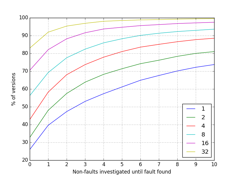
Figure 5. Performance of cl_n on Steimann’s benchmarks with different numbers of faults.

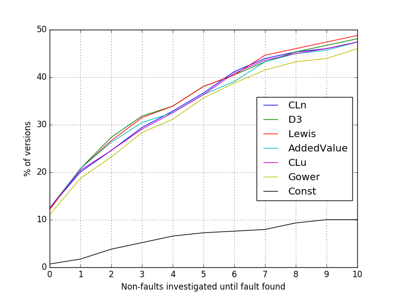
Figure 6. Performance of some methods on Defects4j benchmarks.

We first directly answer our two research questions. First, Which method is the most accurate? For Defects4j cl_n has the best accuracy score (213.6). For Steimann’s benchmarks, cl_u has the best accuracy score (4.9) (cl_n came second with 5.02). Second, Do our new techniques have the best $n$-scores for any $n\in[0,10]$? For Defects4j, cl_n had the best 6-score (41.18). For Steimann’s benchmarks, for all $n\in[0,10]$, cl_u had the best $n$-scores for each of the sets of 4, 8, 16, 32 faults. cl_n had the second best scores in these cases.

We first discuss the results for Defects4j, and begin with the overall accuracy scores. To show the range, we report the measures which were ranked 1, 2, 10, 50, 90, 100. These were cl_n (213.6), D3 (216.36), Lewis (224.79), AddedValue (232.46), cl_u (241.22) Gower (248.72) respectively. The constant measure was ranked last (643.78). We now summarise the $n$-scores for each $n\in[0,10]$. The $n$-scores for a range of methods are presented in Figure 6. We describe the figure as follows. For each method in the legend, a point was plotted at (x, y) if in y% of the versions a fault was localized after investigating x non-faulty lines of code. To show the range of performance across methods, the methods in the legend are associated with the aforementioned methods. Of all 127 methods compared, cl_u did not get the best $n$-score for any of $n\in[0,10]$, and cl_n tied with the best 6-score (41.18 - tied with Dennis, Ochiai, and f9830).

We now discuss the results for Steimann’s benchmarks. We first summarise the overall accuracy scores. To show the range of scores, we report the methods which were ranked 1, 2, 3, 10, 20, 50, 100. These were cl_u (4.9), cl_n (5.02), Klosgen (9.02), SokalSneath4 (9.51), calf, (9.77), Tarantula (10.54), GP23 (15.68). The constant measure came last (38.69). We now summarise accuracy scores on sets of 1, 2, 4, 8, 16, 32 fault programs. On 1-fault programs, Naish received the best accuracy score (9.81). cl_u came 72nd (14.5) and cl_n came 74th (14.69). On each of the sets of versions with multiple faults, cl_u and cl_n came 1st and 2nd respectively, as follows: On 2-fault programs, the top 3 were cl_u (9.87) cl_n and (10.04) and D3 (13.1). On 4-fault programs, the top 3 were cl_u (5.14) cl_n and (5.3) and GeometricMean (10.34). On 8-fault programs, the top 3 were cl_u (2.79) cl_n and (2.94) and Klosgen (7.57). On 16-fault programs, the top 3 were cl_u (1.16) cl_n and (1.24) and AddedValue (6.04). On 32-fault programs, the top 3 were cl_u (0.4) cl_n and (0.44) and Certainty (4.87).

We now summarise the $n$-scores. For each $n\in[0,10]$, and for the set of 1-fault programs, Naish outperformed cl_u or cl_n at every value $n$. For each $n\in[0,10]$, and for the set of 2-fault programs, D3 outperformed cl_u or cl_n at every value of $n$. For each $n\in[0,10]$, and for each of the sets of 4, 8, 16, 32 fault programs, cl_u or cl_n outperformed all sbfl methods at every value of $n$. cl_u and cl_n $n$-scores were always similar (+/- 2 percent of on one another), thus to give an indication of how they perform as the number of faults grows in a program, we present Figure 6. Here, for each of the 1, …, 32 fault programs, a point was plotted on (x, y) if in y% of the versions a fault was localized after investigating x non-faulty lines of code.

In the remainder of this section, we discuss our results. We first discuss differences in value between our evaluative methods (accuracy and $n$-scores). In general, $n$-scores are more important than accuracy from the point of view of an engineer looking for a technique to use in practice. As has been demonstrated in a study by Parnin and Orso, ” programmers will stop inspecting statements, and transition to traditional debugging, if they do not get promising results within the first few statements they inspect” (Parnin and Orso, 2011). $n$-scores are more important from this perspective.

We now discuss the difference in quality between accuracy and $n$-scores. In general, the accuracy scores for all techniques on Defects4j are poor. For instance, using the most accurate method cl_n , one would expect to investigate 213.6 lines of code on average. In contrast, if one limited oneself to investigating fewer than 10 non-faulty lines of code, then one would expect to find a fault almost half the time. For instance, using cl_n we can expect to find a fault 41.68% of the time if one limited oneself to investigating 6 non-faulty lines of code (here, nothing did better than cl_n ). This suggests that accuracy scores were affected by outliers in which the technique only located a fault after investigating many lines of code (we discuss two such outliers below).

We now discuss why methods performed differently on Defects4j as opposed to Steimann. First, in the useable Defects4j versions, the average number of failing test cases way very small, as detailed by Table 2. In contrast, the number of failing test cases in Steimann benchmarks was much larger. We think this improved the performance of different methods, as more failing tests provide more information about the behavior of the fault. Secondly, in the useable Defects4j versions, 38.4% had only a single failing test case. Accordingly, cl_u , cl_n and most sbh’s performed equivalently on these benchmarks in terms of which units get ranked higher/lower, this meant that the performance of high performing methods tended to converge. Thirdly, we emphasize that the uuts in Steimann’s benchmarks were calls to subclasses, which are often larger than lines of code (the units for Defects4j), and thus the scores look better for Steimann’s benchmarks. Fourthly, for Steimann’s benchmarks many of the failing test cases only executed a small part of the overall program. This advantaged our new methods cl_u and cl_u , which take advantage of short failing executions to increase their causal likelihood.

We now discuss the difference in accuracy between cl_u and cl_n . As described earlier, the performance of cl_u is slightly worse than cl_n on Defects4j, where the opposite is observed on Steimann’s benchmarks. We investigated reasons why for this, and after investigating the cases where cl_n outperforms cl_u in terms of accuracy on Defects4j, we discovered there were two major outliers that made cl_u ’s overall accuracy score lower (in Chart-5 cl_u had to investigate 3177 more lines of code, and Math-6 cl_u had to investigate Math-6 1585 more lines of code). For Defects4j, cl_u outperformed cl_n in only two cases, whereas cl_n outperformed cl_u in 50. These results (tentatively) suggest the conclusion that cl_n is better to use in practice when the program and test suite resemble the benchmarks in Defects4j, and cl_u when the program and test suite resemble the benchmarks in Steimann’s benchmarks.

Finally, we think the scores of our new techniques demonstrate they are a strong contender to sbfl heuristics when integrated into a practical fault localisation approach.

4.3. Threats to Validity

Our threats are informed by the recent work of (Just et al., 2014), who perform a similar test on the Defects4j benchmarks, and by Steimann et al., who perform similar experiments on the Steimann benchmarks (Steimann et al., 2013).

The main threat is wrt how well our results generalize to practical instances of fault localisation. Given the variety of programs, faults, test suites, and development styles in ”the wild” it has not yet been shown whether studies of this sort generalize well. Wrt the Steimann benchmarks, there is the additional threat that artificial faults are not good proxies for real faults. Problems of this sort confront many software fault localisation studies (Steimann et al., 2013). To anticipate these problems, we have tried to improve the degree to which our results can generalise by ensuring our experiment was large. To our knowledge our experiment is currently the largest in the literature in terms of three different dimensions: number of methods compared (127+), range of faults studied (1-32), and number of program versions used (50k+).

5. Related Work

The recent survey of Wong et al. (Wong et al., 2016b) identifies the most prominent fault localisation methods to be spectrum based (Abreu et al., 2007; Landsberg et al., 2015; Naish et al., 2011; Lucia et al., 2014; Wong et al., 2014; Eric Wong et al., 2010; Yoo, 2012; Kim et al., 2015; Santelices et al., 2009b), slice based (Agrawal et al., 1995; Zhang et al., 2005; Wong and Qi, 2006; Lei et al., 2012; Weiser, 1981), model based (Mayer and Stumptner, 2008; Wotawa et al., 2002; Yilmaz and Williams, 2007), and mutation-based  (Moon et al., 2014; Papadakis and Le Traon, 2015). For reasons of space, we discuss closely related statistical approaches.

We first discuss sbh, which is one of the most lightweight methods. In general, sbh’s designed to solve the general problem of fault localisation (for programs with any number of faults) are heuristics which estimate how ”suspicious” a given unit is. However, what ”suspicious” means is (to our knowledge) never fully defined. In the absence of an approach which tells us this, research is driven by the development of new measures with improved experimental performance (Abreu et al., 2007; Landsberg et al., 2015; Naish et al., 2011; Lucia et al., 2014; Wong et al., 2014; Eric Wong et al., 2010; Yoo, 2012; Kim et al., 2015; Santelices et al., 2009b). Many of these top-performing measures are presented in Table 1: D3 was developed by raising the numerator of a previously used measure to the power of 3 (Wong et al., 2012c). Zoltar was developed by adding $10000\frac{nfep}{ef}$ to the denominator of a previously used measure (Janssen et al., 2009). GP05 was found using genetic programming (Yoo, 2012). Ochiai was originally designed for Japanese fish classification (Ochiai, 1957; Abreu et al., 2007). In this paper, we have tried to improve upon the theoretical connection between developed measures and the fault localisation problem.

We now discuss theoretical results for sbfl. Theoretical results include proving potentially desirable formal properties of measures and finding equivalence proofs for classes of measures (Xie et al., 2013; Landsberg et al., 2015; Naish et al., 2011; Naish and Lee, 2013; Debroy and Wong, 2011). Yoo et al. have established theoretical results that show that a ”best” performing suspicious measure for sbfl does not exist (Yoo et al., 2014), arguing there is ”no pot of gold at the end of the program spectrum rainbow” in theory. With this result, there remains the problem of providing better formal foundations, and deriving improved measures shown to satisfy more formal properties. Our work in this paper is designed to addresses this.

Two more heavyweight approaches to multiple fault localisation are as follows. Both of these approaches use fault models in their analysis. Here, a fault model is a set of units with the property that each failing trace executes at least one of them. The first is the simple classical approach of Steimann et al. (Steimann and Bertschler, 2009), where the probability of a unit being faulty is the proportion of fault models it is a member of. A second method is Barinel  (Abreu et al., 2009), which uses Bayesian analysis and heuristic policies to estimate the health of uuts, and uses a tool Staccato (Abreu and van Gemund, 2009) to generate large sets of fault models. The main issue confronting these approaches is scalability, given the requirement of generating large sets of fault models. Additionally, in one study the implementation of Barinel was unable to scale to the Steimann benchmarks (Landsberg et al., 2016). We have purposely designed our approach to avoid this issue by having a different definition of a model which facilitates tractable fault localisation methods.

We discuss miscellaneous statistical approaches here. One type of approach uses machine learning, including support vector machines and neural network approaches, to perform fault localisation (Ascari et al., 2009; Wong et al., 2012b). However, these approaches do not make the case that a recourse to machine learning methods is necessary and that a principled approach is impossible. Other approaches include the crosstab-based method of Wong (Wong et al., 2012a), the hypothesis testing approach of Liu (Liu et al., 2006), and the probabilistic program dependence graph approach of Baah (Baah et al., 2008). Landsberg et al. provide an axiomatic setup which uses sbhs in a probabilistic framework, but does not use models (Landsberg et al., 2016).

We now discuss how lightweight statistical methods have been used in the following applications. Firstly, in semi-automated fault localisation in which users inspect code in descending order of suspiciousness (Parnin and Orso, 2011). Secondly, in fully-automated fault localisation subroutines within algorithms which inductively synthesize (such as cegis (Jha and Seshia, 2014)) or repair programs (such as GenProg (Goues et al., 2012)). Thirdly, as a technique combined with other methods (Kim et al., 2015; Xuan and Monperrus, 2014; Baudry et al., 2006; Ju, [n. d.]). Finally, as a potential substitute for heavyweight methods which cannot scale to large programs. Thus, there is a large field of application for the techniques discussed in this paper.

Finally, for the approach of classical probability, the overview of James (Jaynes, 2003), the introduction of Tijms (Henk, 2004), and the measure-theoretic foundations of Kolmogorov (Kolmogorov, 1960) all provided bases upon which to develop our approach.

6. Conclusion

In this paper, we have demonstrated there is a principled formal foundation (Doric) available for statistical fault localisation that does not require recourse to spectrum-based heuristics. In general, Doric opens up a world of different meaningful probabilities which can be reported to the engineer to aid in understanding a faulty program. To illustrate the utility of Doric, we developed two lightweight measures of fault and causal likelihood and integrated the latter into our fault localisation method cl_n . In large-scale experimentation, cl_n was demonstrated to be more accurate when compared with all known 127 sbhs . In particular, on the Steimann benchmarks cl_n was almost twice as accurate as the best performing sbh — you’d expect to find a fault by examining 5.02 methods as opposed to 9.02. cl_n also demonstrated to have the highest 6-score on Defects4j. We think the combined effort demonstrates that our measure of causal likelihood is lightweight, effective and maintains a meaningful connection to fault localisation.

We now discuss directions for future work. First, a major step in our work is to experiment with different weight functions ($w$). There are many ways to do this, so it is our hope there will be as much experimentation over different weights as there has been comparing sbhs. A natural place to start is to define the relative likelihood of a model as a function of the number of faults in that model in conjunction with some given cumulative distribution function. Following work on fault distributions in software (Grbac and Huljenić, 2015), we wish to weigh models with a small number of faults to have a higher relative likelihood. The formal development in this paper lays much of the foundations critical for this step.

Appendix A Proofs

In this appendix, we present the proofs supporting the main text. To simplify, we have put a proof later in our order of presentation if a part of that proof relies on a part of an earlier proof.

To aid in the proofs we introduce some notation. For each $m^{j}\in M$, $m^{j}_{i,k}$ is the value at the $i$th column and $k$th row. $m^{j}_{k}$ is the matrix consisting of the $k$th row of $m^{j}$. For each $t_{k}\in T$ we let $M_{k}$ = {$m^{j}_{k}|1\leq j\leq|M|$}. Intuitively, this is all different $k$th rows of all models. We make use of a concatonation operation $\cdot$ such that $x$ $\cdot$ $y$ is the concatonation of two matrices, and extend the definition such that $M_{i}\cdot M_{j}$ = {$x\cdot y|x\in M_{i}\wedge y\in M_{j}$}. Accordingly, definition 3 is designed to conform to the following assumption $M=M_{1}\cdot M_{2}\cdot...\cdot M_{|T|}$. It is observed that $|M_{k}|$ = $2^{\rho_{k}}-1$ if $t_{k}$ is failing, and 1 otherwise.

Proposition A.1.

Equation 9 follows using the defs.

Proof.

We must show $P(H_{i}\wedge u_{i})=P(H_{i})$. It is sufficient to show $v_{k}(H_{i}\wedge u_{i})$ = $v_{k}(H_{i})$. Thus, it is sufficient to show $v_{k}(H_{i}\wedge u_{i})$ = $v_{k}(H_{i})\cap v_{k}(u_{i})$ (by def. 3.4). Now, $v_{k}(H_{i})\cap v_{k}(u_{i})\subseteq v_{k}(H_{i})$ (as in general $X\cap Y\subseteq X$), thus it remains to show $v_{k}(H_{i})\cap v_{k}(u_{i})$ $\subseteq$ $v_{k}(H_{i})$. It is sufficient to show $v_{k}(u_{i})$ $\subseteq$ $v_{k}(H_{i})$ (as in general $X\subseteq X$). Now, $v_{k}(H_{i})$ = (by the abbreviation for $H_{i}$) $v_{k}(h_{1}\wedge\neg h_{2}\wedge...\wedge\neg h_{|U|-1})$ = (by def. 3.4) $v_{k}(h_{1})\cap v_{k}(\neg h_{2})\cap...\cap\neg v_{k}(h_{|U|-1})$ = $\{m^{j}|m^{j}_{1,k}=2\}\cap\{m^{j}|m^{j}_{1,k}\in\{1,0\}\}\cap\dots$ (by def. 3 and 2). = $\{m^{j}|m^{j}_{1,k}=2\}\cap\{m^{j}|m^{j}_{1,k}\in\{1,0\}\}\cap\dots$ = $\{m^{j}|m^{j}_{1,k}=2\wedge m^{j}_{1,k}\in\{1,0\}\wedge\dots\}$ = $\{m^{j}|m^{j}_{1,k}\in\{1,2\}\wedge m^{j}_{1,k}=2\wedge m^{j}_{1,k}\in\{1,0\}\wedge\dots\}$. A subset of which is $\{m^{j}|m^{j}_{1,k}\in\{1,2\}\}$, which is $v_{k}(u_{i})$ (by def. 3).

Proposition A.2.

Equation 11 follows using the defs.

We sketch the proof for equation 11. $P_{t}(H_{i})$ is equal to $\frac{|v_{t}(H_{i})|}{|M|}$ (by def. 3.6). We first do the top condition of equation 11. Without loss of generality, let $k=1$. Assume $c_{i,1}=e_{1}$ = 1. Now, $M=M_{1}\cdot M_{2}\cdot...\cdot M_{|M|}$ (by A1). Thus, $v_{1}(H_{i})$ = $\{m^{j}_{1}|m^{j}\in v_{1}(H_{i})\}\cdot M_{2}\cdot...\cdot M_{n}$ (as in general, $v_{1}(\phi)$ = $\{m^{j}_{k}\in M_{1}|m^{j}\in v_{k}(\phi)\}\cdot M_{2}\cdot...\cdot Mn$). So, $|v_{1}(H_{i})|$ = $|\{m^{j}_{1}|m^{j}\in v_{1}(H_{i})\}|\times|M_{2}|\times...\times|M_{|T|}|$. So, $|v_{1}(H_{i})|$ = $1\times|M_{2}|\times...\times|M_{|T|}|$ (given if $m^{j},m^{k}\in$ $v_{1}(H_{i})$ then $m^{j}_{1}=m^{k}_{1}$). Thus, $1\times|M_{2}|\times...\times|M_{|T|}|$ / $|M_{1}|\times|M_{2}|\times...\times|M_{|T|}|$. This is equal to $1/|M_{1}|$ (by cancellation), which is equal to $1/(2^{\rho_{1}}-1)$ (given $\rho_{1}=\sum_{i<|U|}c_{i,1}$). We now do the bottom condition (when either $c_{i,1}$ or $e_{1}$ is 0). Accordingly, there are no models in $v_{1}(h_{i})$ (by def. 4), thus no models in $v_{1}(H_{i})$ (by def. 3.4 and $H_{i}$), and so $P_{1}(H_{i})=0$.

Proposition A.3.

Equation 12 follows using the defs.

We must show $P(u_{i})$ = $\sum_{k}c_{i,k}/|T|$. $P(u_{i})$ is equal to $f(u_{i})/|T|$ (by proposition 3.7). The latter is equal to $\sum_{k}f_{k}(u_{i})/|T|$. It remains to show $f_{k}(u_{i})=c_{i,k}$, for both cases when $c_{i,k}$ is 1 or 0 (given $c$ is a Boolean matrix). Assume $c_{i,k}$ is 1. Then for all $m\in M$, $m_{i,k}\in{1,\bullet}$ (by def. 3.1). Thus, $v_{k}(u_{i})=M$ (by def. 3.4). So, $f_{k}(u_{i})$ = 1. Assume $c_{i,k}$ is 0. Then for all $m\in M$, $m_{i,k}=0$ (by def. 3.1). Thus, $v_{k}(u_{i})=M$ (by def. 3.4).

∎

Proposition A.4.

For all $\phi\in L^{*}$, $P(\phi)$ = $\frac{f(\phi)}{|T|}$

Proof.

We must show for all $\phi\in L^{*}$, $P(\phi)$ = $\frac{f(\phi)}{|T|}$. $P(\phi)$ is equal to $\sum_{k}P_{k}(\phi)/|T|$ (by def.3.6). The latter is equal to $\sum_{k}(w(v_{k}(\phi))$ $/w(M))/|T|$ (by def.3.6). Now, $\frac{f(\phi)}{|T|}$ = $\sum_{k}\frac{f_{k}(\phi)}{|T|}$ (by definition of $f$). Thus it is remains to prove $w(v_{k}(\phi))/w(M))=f_{k}(\phi)$. We have two cases to consider, when $f_{k}(\phi)=1$ and when it is 0. We do the former first. Assume $f_{k}(\phi)=1$, then $v_{k}(u_{i})=M$ (by definition of $f$). So $w(v_{k}(\phi))/w(M))$ = $w(M)/w(M)$ = 1. Assume $f_{k}(\phi)=0$, then $v_{k}(\phi)\neq M$. If the latter, then $v_{k}(\phi)=\emptyset$ (as $\phi\in L^{*}$). So $w(v_{k}(\phi))/w(M))$ = $w(\emptyset)/w(M)$ = 0 (by def. of $w$). ∎

Proposition A.5.

Equation 3 follows given indifference

Proof.

Let $v_{k}(\phi)=\{m^{i},\dots,m^{j}\}$ and $M=\{m^{1},\dots,M^{|M|}\}$. Then $P_{k}(\phi)$ = $\sum_{i=1}^{j}w(\{m^{i}\})$ / $\sum_{k=1}^{|M|}w(\{m^{k}\})$ (by Def. 3.6). Now, $w(\{m^{k}\})>0$ for all $m^{k}\in M$ (by the conditions on $w$ and indifference). Given indifference, let $w(\{m^{k}\})$ = $x\times|\{m^{k}\}|$. Then $P_{k}(\phi)$ = $\sum_{i=1}^{j}x|\{m^{i}\}|$ / $\sum_{k=1}^{|M|}x|\{m^{k}\}|$ (by substitution). Thus, $P_{k}(\phi)$ = $x\sum_{i=1}^{j}|\{m^{i}\}|$ / $x\sum_{k=1}^{|M|}|\{m^{k}\}|$ (by distribution). So, $P_{k}(\phi)$ = $\sum_{i=1}^{j}|\{m^{i}\}|$ / $\sum_{k=1}^{|M|}|\{m^{k}\}|$ (by cancellation). Equivalently, $P_{k}(\phi)$ = $|\{m^{i},\dots,m^{j}\}|$ / $|M|$. So, $P_{k}(\phi)$ = $|v_{k}(\phi)|$ / $|M|$ (by substitution). ∎

Proposition A.6.

Let $c$ be a coverage matrix where $c_{i,k}=c_{j,k}=1$ for some $t_{k}\in T$. Then $P(H_{i}|u_{i})<P(H_{i}|u_{i}\wedge\neg h_{j})$.

Proof.

We show $P(H_{i}|u_{i})<P(H_{i}|u_{i}\wedge\neg h_{j})$ given the conditions of the proposition. This is equivalent to $P(H_{i}\wedge u_{i})/P(u_{i})<P(H_{i}\wedge u_{i}\wedge\neg h_{j})/$ $P(u_{i}\wedge\neg h_{j})$ (by $|$-def.). Equivalently, $P(H_{i}\wedge u_{i})/P(u_{i})<P(H_{i}\wedge u_{i})/$ $P(u_{i}\wedge\neg h_{j})$ (given $H_{i}$ implies $\neg h_{j}$). Accordingly, it is sufficient to show $1/P(u_{i})<1/P(u_{i}\wedge\neg h_{j})$. It then suffices to show $P(u_{i})>P(u_{i}\wedge\neg h_{j})$. Equivalently, $\sum_{k}P_{k}(u_{i})/|T|>\sum_{k}P_{k}(u_{i}\wedge\neg h_{j})/|T|$ (by def. 3.6). Equivalently, $\sum_{k}P_{k}(u_{i})>\sum_{k}P_{k}(u_{i}\wedge\neg h_{j})$ (by cancellation). Equivalently, $\sum_{k}|v_{k}(u_{i})|/|M|>\sum_{k}|v_{k}(u_{i}\wedge\neg h_{j})|/|M|$. Equivalently, $\sum_{k}|v_{k}(u_{i})|>\sum_{k}|v_{k}(u_{i}\wedge\neg h_{j})|$ (by cancellation). Equivalently, $\sum_{k}|v_{k}(u_{i})|>\sum_{k}|v_{k}(u_{i})\cap(M-v(h_{j})))|$ (by def. 3.3). It is sufficient to show $M-v(h_{j})\subset$ $v_{k}(u_{i})$. $v_{k}(u_{i})=M$ (given $c_{i,k}=1$). Thus it suffices to show $M-v(h_{j})\subset$ $M$. To prove this, it is sufficient to show $v(h_{j})\neq\emptyset$. This holds given $c_{j,k}=1$ (given the conditions of the proposition and def. 3.1). ∎

Proposition A.7.

Equations 4, 5, &  6 follow given indifference.

Proof.

We sketch the proof here. Equation 4 follows given the definition of $f_{i}$ in Section 3. Equation 6 is similar to the proof for Equation 11. We do the proof for Equation 5 here. As the general proof for this involves syntactically complex formulae, we sketch the proof for reasons of space, and do the case for when there are two test cases $T=\{t_{1},t_{2}\}$ here. $P(\Diamond_{1}h_{i}\vee\Diamond_{2}h_{i})$ = $(1-P(\Diamond_{1}h_{i}))$ $(P(\Diamond_{1}h_{i}))+P(\Diamond_{2}h_{i}))$. The latter expression is equal to $(P(\Diamond_{1}h_{i}))+P(\Diamond_{2}h_{i}))$ - $(P(\Diamond_{1}h_{i})P(\Diamond_{1}h_{i}))$. Thus it is sufficient to prove $P(\Diamond_{1}h_{i}\vee\Diamond_{2}h_{i})$ is equal to that. Now, in general $P(\phi\vee\psi)=P(\phi)+P(\psi)-P(\phi\wedge\psi)$. Thus it suffices to show $P(\Diamond_{1}h_{i})P(\Diamond_{1}h_{i})$ = $P(\Diamond_{1}h_{i}\wedge\Diamond_{1}h_{i})$. It is sufficient to show $|v_{1}(h_{i})\cap v_{2}(h_{i})|/|M|$ = $|v_{1}(h_{i})|/|M|\times|v_{2}(h_{i})|/|M|$. It is sufficient to show $|v_{1}(h_{i})\cap v_{2}(h_{i})|$ = $|v_{1}(h_{i})||v_{2}(h_{i})|$. Now $M=M_{1}\cdot M_{2}$. Thus, for every $m^{j}_{1}\in M_{1}$ there is a paired $m^{j}_{2}\in M_{2}$. Thus $|v_{1}(h_{i})\cap v_{2}(h_{i})|$ = $|v_{1}(h_{i})||v_{2}(h_{i})|$. ∎

References

- (1)
- new ([n. d.]) [n. d.]. MS Windows NT Kernel Description. https://www.newscientist.com/gallery/software-faults/. Accessed: 2010-09-30.
- Abreu and van Gemund (2009) Rui Abreu and Arjan J. C. van Gemund. 2009. A Low-Cost Approximate Minimal Hitting Set Algorithm and its Application to Model-Based Diagnosis. In Abstraction, Reformulation, and Approximation (SARA).
- Abreu et al. (2006) Rui Abreu, Peter Zoeteweij, and Arjan J. C. van Gemund. 2006. An Evaluation of Similarity Coefficients for Software Fault Localization. In PRDC. 39–46.
- Abreu et al. (2007) Rui Abreu, Peter Zoeteweij, and Arjan J. C. van Gemund. 2007. On the Accuracy of Spectrum-based Fault Localization. In TAICPART-MUTATION. IEEE, 89–98.
- Abreu et al. (2009) Rui Abreu, Peter Zoeteweij, and Arjan J. C. van Gemund. 2009. Spectrum-Based Multiple Fault Localization. In ASE. 88–99.
- Agrawal et al. (1995) H. Agrawal, J. R. Horgan, S. London, and W. E. Wong. 1995. Fault localization using execution slices and dataflow tests. Software Reliability Engineering, 1995. Proceedings., Sixth International Symposium on, 143–151.
- Ascari et al. (2009) L. C. Ascari, L. Y. Araki, A. R. T. Pozo, and S. R. Vergilio. 2009. Exploring machine learning techniques for fault localization. In 2009 10th Latin American Test Workshop. 1–6.
- Baah et al. (2008) George K. Baah, Andy Podgurski, and Mary Jean Harrold. 2008. The Probabilistic Program Dependence Graph and Its Application to Fault Diagnosis (ISSTA ’08). 189–200.
- Baudry et al. (2006) Benoit Baudry, Franck Fleurey, and Yves Le Traon. 2006. Improving Test Suites for Efficient Fault Localization. In ICSE. ACM, 82–91.
- de Souza et al. (2016) Higor Amario de Souza, Marcos Lordello Chaim, and Fabio Kon. 2016. Spectrum-based Software Fault Localization: A Survey of Techniques, Advances, and Challenges. CoRR (2016).
- Debroy and Wong (2011) Vidroha Debroy and W. Eric Wong. 2011. On the equivalence of certain fault localization techniques. In Proceedings of the 2011 ACM Symposium on Applied Computing (SAC). 1457–1463. https://doi.org/10.1145/1982185.1982498
- DiGiuseppe and Jones (2011) Nicholas DiGiuseppe and James A. Jones. 2011. On the Influence of Multiple Faults on Coverage-based Fault Localization. In ISSTA. ACM, 210–220.
- Eric Wong et al. (2010) W. Eric Wong, Vidroha Debroy, and Byoungju Choi. 2010. A Family of Code Coverage-based Heuristics for Effective Fault Localization. JSS 83, 2 (2010), 188–208.
- Goues et al. (2012) Claire Le Goues, ThanhVu Nguyen, Stephanie Forrest, and Westley Weimer. 2012. GenProg: A Generic Method for Automatic Software Repair. IEEE Trans. Software Eng. 38, 1 (2012), 54–72.
- Grbac and Huljenić (2015) Tihana Galinac Grbac and Darko Huljenić. 2015. On the probability distribution of faults in complex software systems. Information and Software Technology 58 (2015), 250–258.
- Groce (2004) Alex Groce. 2004. Error Explanation with Distance Metrics. In TACAS (LNCS), Vol. 2988. Springer, 108–122.
- Henk (2004) Tijms Henk. 2004. Understanding Probability.
- Janssen et al. (2009) Tom Janssen, Rui Abreu, and Arjan J. C. van Gemund. 2009. Zoltar: a spectrum-based fault localization tool. In SINTER. ACM, 23–30.
- Jaynes (2003) E. T. Jaynes. 2003. Probability theory: The logic of science. Cambridge University Press, Cambridge.
- Jha and Seshia (2014) Susmit Jha and Sanjit A. Seshia. 2014. Are There Good Mistakes? A Theoretical Analysis of CEGIS. In 3rd Workshop on Synthesis (SYNT). 84–99.
- Jones et al. (2002) James A. Jones, Mary Jean Harrold, and John Stasko. 2002. Visualization of Test Information to Assist Fault Localization. In Proceedings of the 24th International Conference on Software Engineering (ICSE ’02). ACM, 467–477. https://doi.org/10.1145/581339.581397
- Ju ([n. d.]) Xiaolin et al. Ju. [n. d.]. ([n. d.]). https://doi.org/10.1016/j.jss.2013.11.1109
- Just et al. (2014) René Just, Darioush Jalali, and Michael D. Ernst. 2014. Defects4J: A Database of Existing Faults to Enable Controlled Testing Studies for Java Programs (ISSTA 2014). 437–440.
- Kim et al. (2015) Jeongho Kim, Jonghee Park, and Eunseok Lee. 2015. A New Hybrid Algorithm for Software Fault Localization. In IMCOM. ACM, 50:1–50:8.
- Kolmogorov (1960) Andrey N. Kolmogorov. 1960. Foundations of the Theory of Probability (2 ed.). Chelsea Pub Co. http://www.clrc.rhul.ac.uk/resources/fop/Theory%20of%20Probability%20(small).pdf
- Landsberg (2016) David Landsberg. 2016. Methods and Measures for Statistical Fault Localisation (doctoral thesis). Ph.D. Dissertation. University of Oxford.
- Landsberg et al. (2016) David Landsberg, Hana Chockler, and Daniel Kroening. 2016. Probabilistic Fault Localisation. In Haifa Verification Conference. 65–81.
- Landsberg et al. (2015) David Landsberg, Hana Chockler, Daniel Kroening, and Matt Lewis. 2015. Evaluation of Measures for Statistical Fault Localisation and an Optimising Scheme. In FASE. LNCS, Vol. 9033. Springer, 115–129.
- Lei et al. (2012) Yan Lei, Xiaoguang Mao, Ziying Dai, and Chengsong Wang. 2012. Effective Statistical Fault Localization Using Program Slices.. In COMPSAC. IEEE Computer Society, 1–10.
- Liblit et al. (2005) Ben Liblit, Mayur Naik, Alice X. Zheng, Alex Aiken, and Michael I. Jordan. 2005. Scalable Statistical Bug Isolation. SIGPLAN Not. (2005), 15–26.
- Liu et al. (2006) Chao Liu, Long Fei, Xifeng Yan, Jiawei Han, and Samuel P. Midkiff. 2006. Statistical Debugging: A Hypothesis Testing-Based Approach. IEEE Trans. Softw. Eng. 32, 10 (2006), 831–848.
- Lucia et al. (2014) Lucia, David Lo, Lingxiao Jiang, Ferdian Thung, and Aditya Budi. 2014. Extended comprehensive study of association measures for fault localization. Journal of Software: Evolution and Process 26, 2 (2014), 172–219.
- Mayer and Stumptner (2008) W. Mayer and M. Stumptner. 2008. Evaluating Models for Model-Based Debugging. In ASE. 128–137.
- Moon et al. (2014) Seokhyeon Moon, Yunho Kim, Moonzoo Kim, and Shin Yoo. 2014. Ask the Mutants: Mutating Faulty Programs for Fault Localization (ICST ’14). 153–162.
- Naish and Lee (2013) Lee Naish and Hua Jie Lee. 2013. Duals in Spectral Fault Localization. In Australian Conference on Software Engineering (ASWEC). IEEE, 51–59.
- Naish et al. (2011) Lee Naish, Hua Jie Lee, and Kotagiri Ramamohanarao. 2011. A Model for Spectra-based Software Diagnosis. ACM Trans. Softw. Eng. Methodol. (2011), 1–11.
- Ochiai (1957) A. Ochiai. 1957. Zoogeographical Studies on the Soleoid Fishes Found in Japan and its Neighboring Regions. Bull. Jap. Soc. sci. Fish. (1957), 526–530.
- Papadakis and Le Traon (2015) Mike Papadakis and Yves Le Traon. 2015. Metallaxis-FL: Mutation-based Fault Localization. Softw. Test. Verif. Reliab. 25, 5-7 (Aug. 2015), 24.
- Parnin and Orso (2011) Chris Parnin and Alessandro Orso. 2011. Are Automated Debugging Techniques Actually Helping Programmers?. In International Symposium on Software Testing and Analysis (ISSTA). 199–209.
- Popper (2005) Karl Popper. 2005. The logic of scientific discovery. Routledge.
- Santelices et al. (2009a) R. Santelices, J. A. Jones, Yanbing Yu, and M. J. Harrold. 2009a. Lightweight fault-localization using multiple coverage types. In ICSE. 56–66.
- Santelices et al. (2009b) Raul Santelices, James A. Jones, Yanbing Yu, and Mary Jean Harrold. 2009b. Lightweight Fault-localization Using Multiple Coverage Types (ICSE ’09). 11.
- Steimann and Bertschler (2009) Friedrich Steimann and Mario Bertschler. 2009. A Simple Coverage-Based Locator for Multiple Faults.. In ICST (2009-12-23). IEEE Computer Society, 366–375.
- Steimann and Frenkel (2012) Friedrich Steimann and Marcus Frenkel. 2012. Improving Coverage-Based Localization of Multiple Faults Using Algorithms from Integer Linear Programming. In ISSRE November 27-30. 121–130.
- Steimann et al. (2013) Friedrich Steimann, Marcus Frenkel, and Rui Abreu. 2013. Threats to the Validity and Value of Empirical Assessments of the Accuracy of Coverage-based Fault Locators. In ISSTA. ACM, 314–324.
- Weiser (1981) Mark Weiser. 1981. Program Slicing. In ICSE. IEEE Press, 439–449.
- Wong et al. (2014) W.E. Wong, V. Debroy, Ruizhi Gao, and Yihao Li. 2014. The DStar Method for Effective Software Fault Localization. Reliability, IEEE Transactions on 63, 1 (2014), 290–308.
- Wong et al. (2012b) W. E. Wong, V. Debroy, R. Golden, X. Xu, and B. Thuraisingham. 2012b. Effective Software Fault Localization Using an RBF Neural Network. IEEE Transactions on Reliability 61, 1 (March 2012), 149–169.
- Wong et al. (2012c) W. E. Wong, V. Debroy, Y. Li, and R. Gao. 2012c. Software Fault Localization Using DStar (D*). In 2012 IEEE Sixth International Conference on Software Security and Reliability. 21–30.
- Wong et al. (2012a) W. Eric Wong, Vidroha Debroy, and Dianxiang Xu. 2012a. Towards Better Fault Localization: A Crosstab-Based Statistical Approach. IEEE Trans. Systems, Man, and Cybernetics, Part C 42, 3 (2012), 378–396. https://doi.org/10.1109/TSMCC.2011.2118751
- Wong et al. (2016a) W. E. Wong, R. Gao, Y. Li, R. Abreu, and F. Wotawa. 2016a. A Survey on Software Fault Localization. IEEE Transactions on Software Engineering 99 (2016).
- Wong et al. (2016b) W. Eric Wong, Ruizhi Gao, Yihao Li, Rui Abreu, and Franz Wotawa. 2016b. A Survey on Software Fault Localization. IEEE Trans. Softw. Eng. 42, 8 (Aug. 2016), 34.
- Wong and Qi (2006) W. Eric Wong and Yu Qi. 2006. Effective program debugging based on execution slices and inter-block data dependency. JSS (2006), 891–903.
- Wong et al. (2007) W. Eric Wong, Yu Qi, Lei Zhao, and Kai-Yuan Cai. 2007. Effective Fault Localization Using Code Coverage. In COMPSAC. 449–456.
- Wotawa et al. (2002) Franz Wotawa, Markus Stumptner, and Wolfgang Mayer. 2002. Model-Based Debugging or How to Diagnose Programs Automatically. In Developments in Applied Artificial Intelligence. LNCS, Vol. 2358. 746–757.
- Xie et al. (2013) Xiaoyuan Xie, Tsong Yueh Chen, Fei-Ching Kuo, and Baowen Xu. 2013. A Theoretical Analysis of the Risk Evaluation Formulas for Spectrum-based Fault Localization. ACM Trans. Softw. Eng. Methodol. (2013), 31:1–31:40.
- Xuan and Monperrus (2014) Jifeng Xuan and Martin Monperrus. 2014. Learning to Combine Multiple Ranking Metrics for Fault Localization. In ICSME. https://doi.org/10.1109/ICSME.2014.41
- Yilmaz and Williams (2007) Cemal Yilmaz and Clay Williams. 2007. An Automated Model-based Debugging Approach. In ASE. ACM, 174–183.
- Yoo (2012) Shin Yoo. 2012. Evolving Human Competitive Spectra-Based Fault Localisation Techniques. In SSBSE (LNCS), Vol. 7515. 244–258.
- Yoo et al. (2014) S. Yoo, X. Xiaoyuan, F. Kuo, T. Chen, Y. Tsong Yueh, and M. Harman. 2014. No pot of gold at the end of program spectrum rainbow: Greatest risk evaluation formula does not exist. Department of Computer Science, University College London (2014).
- Zhang et al. (2005) Xiangyu Zhang, Haifeng He, Neelam Gupta, and Rajiv Gupta. 2005. Experimental Evaluation of Using Dynamic Slices for Fault Location (AADEBUG). ACM, 33–42.