Photon assisted braiding of Majorana fermions in a cavity

Abstract

We study the dynamical process of braiding Majorana bound states in the presence of the coupling to photons in a microwave cavity. We show theoretically that the $\pi/4$ phase associated with the braiding of Majoranas, as well as the parity of the ground state are imprinted into the photonic field of the cavity, which can be detected by dispersive readouts techniques. These manifestations are purely dynamical, they occur in the absence of any splitting of the MBS that are exchanged, and they disappear in the static setups studied previously. Conversely, the cavity can affect the braiding phase, which in turn should allow for cavity controlled braiding.

Introduction.— Braiding of non-Abelian anyons lies at the heart of topological quantum information processing Nayak et al. (2008). One promising class of non-abelian anyons are the Majorana bound states (MBS) that emerge in the so called topological superconductors as zero-energy quasiparticles Kitaev (2001); Das Sarma et al. (2015); Aasen et al. (2016). In recent years there have been a great deal of excitement towards detecting and manipulating MBS in various condensed matter platforms Alicea (2012); Leijnse and Flensberg (2012); Elliott and Franz (2015); Aguado (2017). In particular, implementations based on one-dimensional (1D) semiconducting wires (SW) have attracted the most attention. Following theoretical proposals Lutchyn et al. (2010); Oreg et al. (2010), several experiments Mourik et al. (2012); Deng et al. (2012); Das et al. (2012); Churchill et al. (2013); Albrecht et al. (2016); Deng et al. (2016); Nichele et al. (2017); Zhang and et al. (2018) have reported characteristic transport signatures in the form of a zero-bias conductance peak compatible with the presence of zero-energy MBS (see Ref. Lutchyn et al. (2018) for a recent review). Nevertheless, the puzzling question of whether such zero-bias peaks are due to MBS is still under debate Liu et al. (2017); Moore et al. (2018) and other direct measurable manifestations of Majorana physics are timely.

The smoking gun feature associated with the MBS is their exchange, or braiding statistics: moving these quasiparticles around each other and exchanging their positions will implement, within the degenerate subspace they pertain to, non-Abelian unitary transformations that depend only on the topology of the trajectories Kitaev (2003); Alicea et al. (2011); Sau et al. (2011); van Heck et al. (2012). Such unitary transforms are more robust against decoherence and dephasing due to local environments, as opposed to quantum computing with conventional qubits (although recent works show that such protection might be fragile when going beyond the adiabatic approximation or assuming a coupling of the MBS to external baths Pedrocchi and DiVincenzo (2015); Pedrocchi et al. (2015); Knapp et al. (2016); Bauer et al. (2018); Nag and Sau (2018)). In order to detect the Majorana signatures, as well as to manipulate the braiding of the MBS, one needs to resort various interference schemes, and eventually lift the ground state degeneracy, thus making MBS interact Alicea (2012); Aasen et al. (2016); Das Sarma et al. (2015).

In this Letter, we analyze the braiding of Majorana fermions in a tri-junction geometry assisted by photons in a cavity quantum electrodynamics (cQED) setup. We show that both the parity of the ground state and the Berry phase associated with the braiding statistics imprint into the cavity field, which in turn can be addressed by conventional dispersive readouts techniques. The present Berry phase coupling mechanism, which is due to the interplay of dynamics during braiding and the non-locality of the photonic field, works even when the lowest energy subspace spanned by the Majorana fermions is degenerate at all times. These effects are purely dynamical and do not have any static analogue (e.g. by comparing the beginning and the end of the braiding by cQED spectroscopy).

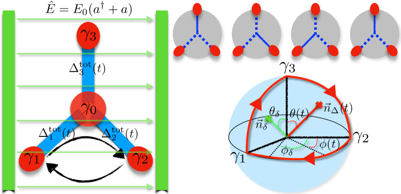
Figure 1: Sketch of the system and the cavity-assisted Majorana braiding (exchange) process of the MBS $\gamma_{1}$ and $\gamma_{2}$. Left: The Y junction with the end $\gamma_{i}$, $i=1,2,3$, and the middle $\gamma_{0}$ MBS, along with the couplings $\Delta_{i}^{\rm tot}(t)=\Delta_{i}(t)+\delta_{i}(a^{\dagger}+a)$ in the presence of the cavity field $\hat{E}$ (green). Right: the braiding steps, with the dashed line $i$ corresponding to a splitting $\Delta_{i}\gg\Delta_{j}$, with $i\neq j$ (top), and the evolution of the vector $\vec{n}_{\Delta}(t)$ in Eq. (1) on the Bloch sphere during the braiding process (bottom). The octant spanned by this vector connects to the Berry phase accumulated by the ground state wavefunction that pertains to the Majorana braiding statistics.

System and Model Hamiltonian.— We consider a Majorana Y junction coupled to the electromagnetic field inside a microwave cavity, as depicted in Fig. 1. The time-dependent effective Hamiltonian describing the Y junction coupled to the cavity reads Karzig et al. (2016):

$$H_{\rm Y}(t) =\frac{i}{2}\gamma_{0}\vec{\Delta^{\rm tot}}(t)\cdot\vec{\gamma}+\omega_{0}a^{\dagger}a\,,$$

$$\vec{\Delta}^{\rm tot}(t) =\vec{\Delta}(t)+\vec{\delta}(a^{\dagger}+a)\,,$$ (1)

where $\gamma_{0}$ stands for the middle MBS (in the center of the junction), $\vec{\gamma}=(\gamma_{1},\gamma_{2},\gamma_{3})$ and $\vec{\Delta}=(\Delta_{1},\Delta_{2},\Delta_{3})$, with $\gamma_{i}$ and $\Delta_{i}$ being the outer MBS and the coupling strengths between $\gamma_{0}$ and $\gamma_{i}$, with $i=1,2,3$. Moreover, $\vec{\delta}=(\delta_{1},\delta_{2},\delta_{3})$ so that $\delta_{i}=\alpha_{i}\Delta_{i}$ for $i=1,2,3$, with $\alpha_{i}$ the weights of the couplings, so that $\delta_{i}$ vanish when $\Delta_{i}$ vanishes, as expected for far apart Majoranas Knapp et al. (2016); Nag and Sau (2018). Finally, $a$ ($a^{\dagger}$) the annihilation (creation) operators for the photons, and $\omega_{0}$ is the cavity frequency.

Next we introduce usual fermionic operators in terms of the Majorana ones $c_{1}=(\gamma_{1}-i\gamma_{2})/2$ and $c_{2}=(\gamma_{0}-i\gamma_{3})/2$, which in turn allows us to write the Majorana Hamiltonian only in the basis $\{|00\rangle,c_{1}^{\dagger}|00\rangle=|10\rangle,c_{2}^{\dagger}|01\rangle=|00\rangle,c_{1}^{\dagger}c_{2}^{\dagger}|00\rangle=|11\rangle\}$ (see SMTrif and Simon (2018) for details):

$$H_{\rm Y}^{\tau}(t) =\frac{1}{2}\vec{\Delta}_{\tau}^{\rm tot}(t)\cdot\vec{\sigma}+\omega_{0}a^{\dagger}a\leavevmode\nobreak\ ,$$ (2)

with $\vec{\Delta}_{\tau}^{\rm tot}(t)=[-\Delta_{2,\tau}^{\rm tot}(t),\tau\Delta_{1,\tau}^{\rm tot}(t),\Delta_{3,\tau}^{\rm tot}(t)]$, and where the Pauli matrices $\sigma_{x,y,z}$ acts within the same parity states $\tau=\pm$, the eigenvalues of the parity operator $\tau_{z}=\gamma_{0}\gamma_{1}\gamma_{2}\gamma_{3}$. We see that the pair of states $\{|00\rangle,|11\rangle\}$ and $\{|01\rangle,|10\rangle\}$ do not couple with each other, which is a consequence of the parity conservation in the system. The Hamiltonian in Eq. (2) describes the more common spin $1/2$ coupled to a cavity mode (similar to the Rabi model).

It is instructive to work in spherical coordinates, and define $\vec{\Delta}_{\tau}(t)=\Delta(t)\,\vec{n}^{\tau}_{\Delta}$, and $\vec{\delta}_{\tau}=\delta\,\vec{n}_{\delta}^{\tau}$, with $\Delta(t)=\sqrt{\sum_{i}\Delta_{i}^{2}(t)}$, $\delta(t)=\sqrt{\sum_{i}\delta_{i}^{2}(t)}$, and $\vec{n}^{\tau}_{\alpha}=(\sin{\theta_{\alpha}}\cos{\phi_{\alpha}},\tau\sin{\theta_{\alpha}}\sin{\phi_{\alpha}},\cos{\theta_{\alpha}})$, where $\alpha=\Delta,\delta$ (nevertheless, in the following we drop the $\Delta$ index from the angles of $\vec{n}_{\Delta}^{\tau}$). We see that the instantaneous ground state for each of the two parities in the absence of the coupling to the cavity are degenerate, with energy $E_{gs}(t)\equiv-\Delta(t)$. In the following, we assume that all manipulations are adiabatic, or $\dot{\Delta}(t)/\Delta(t)\gg\Delta(t)$ at all times, so that there are no real excitations outside the degenerate subspace and the system always stays in the ground state.

Rotating frame description.— In order to describe the braiding in the adiabatic limit, we perform a time-dependent unitary transformation $A_{\tau}(t)$ on the Y junction Hamiltonian, where the columns of the matrix $A_{\tau}(t)$ are given by the instantaneous eigenstates of $\vec{\Delta}_{\tau}(t)\cdot\vec{\sigma}$. The new transformed Hamiltonian becomes $\tilde{H}_{\rm Y}(t)=A_{\tau}^{\dagger}(t)H_{\rm Y}(t)A_{\tau}(t)-iA^{\dagger}_{\tau}(t)\partial_{t}A_{\tau}(t)$, or in more details Trif and Simon (2018):

$$\!\tilde{H}_{\rm Y}^{\tau}(t) =\frac{\Delta(t)}{2}\sigma_{z}+\tau\frac{\dot{\phi}}{2}(1+\cos{\theta}\sigma_{z}+\sin{\theta}\sigma_{x})$$

$$\!\!\!\!\!\!+\frac{\dot{\theta}}{2}\sigma_{y}+A_{\tau}^{\dagger}(t)[\vec{\delta}_{\tau}(t)\cdot\vec{\sigma}]A_{\tau}(t)(a^{\dagger}+a)+\omega_{0}a^{\dagger}a\,.$$ (3)

We now proceed with several approximations. First, in the adiabatic limit, we can neglect the terms $\propto\dot{\phi}\sigma_{x}$ and $\propto\dot{\theta}\sigma_{y}$ above, as they act in higher order in perturbation theory in $1/\Delta(t)$, while the term $\propto\dot{\phi}\sigma_{z}$ is diagonal and responsible for the Berry phase contribution to the dynamics. Second, we assume the weak coupling limit, and perform the rotating wave approximation (RWA) which means we keep only the rotating terms in the above transformed Hamiltonian. Putting all together, we get the full RWA (time-dependent) Hamiltonian

$$\!\!\tilde{H}^{\tau}_{\rm Y}(t) \approx\frac{1}{2}\Delta^{\rm eff}_{\tau}(t)\sigma_{z}+[\tilde{\delta}_{\tau}(t)a\sigma_{+}+{\rm h.c.}]+\omega_{0}a^{\dagger}a\,,$$ (4)

$$\tilde{\delta}_{\tau}(t) =\delta(t)\left[\cos{\theta_{\delta}}\sin{\theta}-\sin{\theta_{\delta}}\cos{\theta}\cos{(\phi-\phi_{\delta})}\right.$$

$$\left.+i\tau\sin{\theta_{\delta}}\sin{(\phi-\phi_{\delta})}\right]/2\,,$$ (5)

where $\Delta^{\rm eff}_{\tau}(t)=\Delta(t)+\tau\dot{\phi}\cos{\theta}$. We see that in this description, the effective Majorana splitting, $\Delta^{\rm eff}_{\tau}(t)$, contains a Berry phase contribution with opposite signs for opposite parities $\tau$, and that $\tilde{\delta}_{-}(t)=\tilde{\delta}^{*}_{+}(t)$, which also implies that $|\tilde{\delta}_{+}(t)|=|\tilde{\delta}_{-}(t)|\equiv\tilde{\delta}(t)$ (independent of $\tau$). This Hamiltonian, which is of Jaynes Cummings type, only couples the states within the pairs $\{|n\uparrow\rangle,|n+1\downarrow\rangle\}$, with $n$ the number of photons in the cavity. Moreover, we can write $\tilde{\delta}_{\tau}=\tilde{\delta}(t)\exp{[i\Phi_{\tau}(t)]}$, with $\Phi_{\tau}(t)=\arg{\tilde{\delta}_{\tau}(t)}\equiv\tau\Phi(t)$, i.e. the spin directly affects the photonic field by adding a time and parity dependent phase. In the static case ($\dot{\phi}=0$), the eigenspectrum is the same for the two parities:

$$\epsilon_{n,\tau}=(n+1/2)\omega_{0}\pm\frac{1}{2}\sqrt{(\Delta-\omega_{0})^{2}+4|\tilde{\delta}|^{2}(n+1)},$$ (6)

and thus the cavity cannot discriminate between the two. Note that in this limit, some overlapping between the Majoranas and thus a splitting of the MBS is required for the cavity to be sensitive to the parity Dmytruk et al. (2015); Dartiailh et al. (2017). Nevertheless, the initial degenerate states built from the MBS become dressed by the photonic field to give rise to degenerate Majorana polaritonic states Trif and Tserkovnyak (2012). Switching on the dynamics implies manipulating the Majorana polaritonic state, either in the resonant or the dispersive regime. In this work, we only focus on the latter, which allows for detection of the braiding statistics while we leave the resonant case for a future study (in such a case the braiding could be even manipulated by means of the cavity).

Dispersive time-dependent Hamiltonian.— Next we address the case of large detuning, quantified by the conditions $\delta\ll|\Delta(t)-\omega|$. The coupling term $\propto\delta$ is now off-diagonal, and we can treat it in time-dependent perturbation theory. For that, we perform a time-dependent Schrieffer-Wolff unitary transformation $U_{\tau}(t)=\exp{[S_{\tau}(t)]}$, with $S_{\tau}^{\dagger}(t)=-S_{\tau}(t)$ on the Hamiltonian $\tilde{H}_{\rm Y}(t)$, chosen as $S_{\tau}(t)=\tilde{e}_{\tau}(t)\sigma_{+}a-\tilde{e}_{\tau}^{*}a^{\dagger}\sigma_{-}$ Goldin and Avishai (2000) so that, up to second order in $\delta$, the effective Hamiltonian reads:

$$\!\!\!\tilde{H}^{\tau}_{\rm Y}(t)\approx\frac{1}{2}\Delta^{\rm eff}_{\tau}(t)\sigma_{z}+g_{\tau}(t)\left(a^{\dagger}a+\frac{1}{2}\right)\sigma_{z}+\omega_{0}a^{\dagger}a\,,$$ (7)

with $g_{\tau}(t)={\mathcal{R}e}[\tilde{\delta}_{\tau}(t)\tilde{e}^{*}_{\tau}(t)]$, and where $\tilde{e}_{\tau}(t)$ is found from the equation

$$[\omega_{0}-\Delta^{\rm eff}_{\tau}(t)]\tilde{e}_{\tau}(t)+\tilde{\delta}_{\tau}(t)+i\dot{\tilde{e}}_{\tau}(t)=0.$$ (8)

In the following, we focus only on cyclic (periodic) trajectories, so that $\tilde{H}^{\tau}_{\rm Y}(t+T)=\tilde{H}^{\tau}_{\rm Y}(t)$, with $T=2\pi/\Omega$ the period of the drive (and $\Omega$ the corresponding frequency). In such a case, the solution to the equation (8) is found as

$$\tilde{e}_{\tau}(t)=\sum_{n}\frac{\tilde{\delta}_{\tau,n}e^{in\Omega t}}{\Delta_{0}-\omega_{0}+(n+\tau\gamma_{B}/2\pi)\Omega}\,,$$ (9)

where $\tilde{\delta}_{\tau,n}=(1/T)\int_{0}^{T}dt\tilde{\delta}_{\tau}(t)\exp{(-2i\pi nt/T)}$ are the Fourier components of $\tilde{\delta}_{\tau}(t)$, $\Delta_{0}=(1/T)\int_{0}^{T}dt\Delta(t)$ is the average energy of the effective spin over one period $T$, while $\gamma_{B}\equiv\gamma_{B}^{\uparrow}-\gamma_{B}^{\downarrow}$ denotes the difference of the Berry phase associated with the spin up and spin down trajectories during the cycle. The (spin-dependent) photonic evolution operator during one cycle becomes $U_{\rm eff}(T)=\exp{[-ig^{\tau}_{\gamma_{B}}Ta^{\dagger}a\sigma_{z}]}$, with $g^{\tau}_{\gamma_{B}}=(1/T)\int_{0}^{T}dtg_{\tau}(t)$ Trif and Simon (2018) or:

$$\!g^{\tau}_{\gamma_{B}}(\omega_{0},\Omega)=\sum_{n}\frac{|\tilde{\delta}_{r,n}|^{2}+|\tilde{\delta}_{i,n}|^{2}+2\tau{\mathcal{I}m}[\tilde{\delta}_{r,n}\tilde{\delta}^{*}_{i,n}]}{\Delta_{0}-\omega_{0}+(n+\tau\gamma_{B}/2\pi)\Omega}\,,$$ (10)

where $\tilde{\delta}_{r(i),n}$ are the $n$-th Fourier components of the real (imaginary) parts of $\tilde{\delta}_{\tau}(t)$. This is one of our main results: the ground state ($\sigma_{z}=-1$) parity and the associated Berry phases imprints into the photonic field evolution operator during one braiding period $T$. The effect of the parity is two-fold: it affects the matrix elements $\tilde{\delta}_{n}$ in the numerator, and it enters in the denominator via the Berry phase. While the denominator has a very simple (universal) form in terms of the parity via the Berry phase, that seems not to be the case for the numerator. To put these two contributions on equal footing, we note that generally $|\tilde{\delta}(t+T)|=|\tilde{\delta}(t)|$, and $\Phi(t+T)=2\pi k+\Phi(t)$, with $k\in{\mathcal{Z}}$ being the number of times the phase $\Phi(t)$ winds during one period $T$. Writing $\tilde{\delta}_{\tau}(t)\approx\delta_{0}\exp{(ik\tau\Omega t)}$, with $\delta_{0}=(1/T)\int_{0}^{T}d\tau|\tilde{\delta}(t)|$, we obtain:

$$g_{\gamma_{B}}^{\tau}(\omega_{0},\Omega)\approx\frac{\delta_{0}^{2}}{\Delta_{0}-\omega_{0}+\tau(k+\gamma_{B}/2\pi)\Omega}\,,$$ (11)

from which we can now simply read the two parity dependent effects: one contribution from the Berry phase of the effective spin, and another contribution from the winding number $k$ of the phase $\Phi(t)$. The static case, corresponding to $\gamma_{B}=2\pi$ and $k=-1$, results in no difference between the two parities, as expected. Note that close to resonances, the perturbative calculation presented above breaks down. However, as shown later, in the presence of dissipation the parity-dependent resonances can be probed.

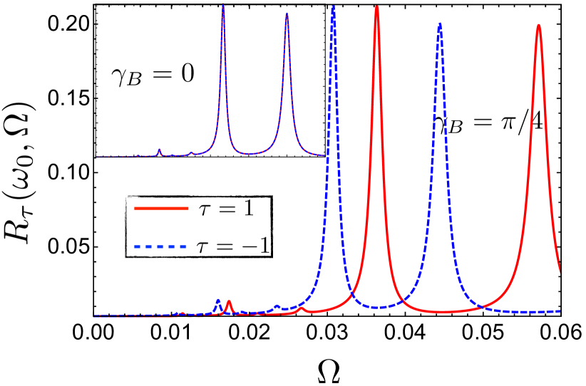
Figure 2: Dependence of the reflection coefficient $R_{\tau}(\omega_{0},\Omega)$ with respect to the braiding frequency $\Omega$ for the two parities $\tau=\pm 1$. In the main (inset) plot we show $R_{\tau}(\Omega)$ with the Berry phase contribution $\gamma_{B}=\pi/4$ included (neglected) in the reflection coefficient. The red (full) and the blue (dashed) correspond to parity $\tau=1$ and $\tau=-1$, respectively. The position of the peaks shift according to Eq. (15), for the braiding trajectory $\gamma_{B}=\pi/4$ (main), while they coincide at $\gamma_{B}=0$ (inset). We consider $\omega=1$, $\Delta_{0}=1.1$, $\kappa=\Gamma=0.002$, as well as $\alpha_{1}=\alpha_{2}=0$, and $\alpha_{3}=0.01$, with all energies expressed in terms of the cavity frequency $\omega_{0}$.

Majorana braiding.— Here we describe briefly the specific implementation of the braiding (exchanging) of the Majorana fermions $\gamma_{1}$ and $\gamma_{2}$. For simplicity, we assume that $\Delta(t)=\Delta_{0}$ is constant during the entire dynamics, and consider the following steps showed in Fig. 1: ${\bm{\Delta}}(t)=\Delta_{0}[0,\sin{\theta(t)},\cos{\theta(t)}]$, for $t\in[0,T/3)$, ${\bm{\Delta}}(t)=\Delta_{0}[\sin{\phi(t)},\cos{\phi(t)},0]$, for $t\in[T/3,2T/3)$, and ${\bm{\Delta}}(t)=\Delta_{0}[\sin{\theta(t)},0,\cos\theta(t)]$, for $t\in[2T/3,T)$, with $\theta(0)=\theta(T)=\phi(T/3)=0$, $\theta(T/3)=\phi(2T/3)=\pi/2$. As showed, for example, in Ref. Karzig et al. (2016), this corresponds to the exchange of the MBS $\gamma_{1}$ and $\gamma_{2}$. The specific implementation for $\theta(t)$ and $\phi(t)$ strongly affects the validity of the adiabatic approximation, especially at the turning points Knapp et al. (2016); Nag and Sau (2018). We disregard such diabatic effects in this work, and for simplicity assume that $\theta(t),\phi(t)=\Omega t$ on the intervals over which they vary. In the spin language, the Berry phase accumulated by the ground state wavefunction of parity $\tau=\pm$ for a path ${\mathcal{C}}$ on the sphere in Fig. 1 is calculated from

$$\gamma_{B,\tau}=\frac{1}{2}\int_{{\mathcal{C}}}d\phi_{\Delta}[1+\tau\cos{\theta}_{\Delta}(t)]\,,$$ (12)

which for the braiding path leads to $\gamma_{B,\tau}=\tau\pi/4$. Using that same prescription allows us to evaluate $\tilde{\delta}_{\tau,n}$ that enter the photonic evolution operator $U_{\rm eff}(T)$, which will be discussed in the next part. We note that in Ref. Karzig et al., 2016 various other paths were studied besides the one pertaining to braiding of MBS, such as the $\pi/8$ magic gate. Our prescription applies for that case too, and such phases could be imprinted into the photonic field and eventually read, for example, by measuring the output field from the cavity, as discussed in the next part.

Detection and Dissipation.— Here we briefly discuss the detection of the cavity field, and consequently the braiding via the the input-output scheme by adding the coupling of the cavity to the external world (or stripline) $H_{c-b}=-i\sum_{k}(f_{k}a^{\dagger}b_{k}-f_{k}^{*}b^{\dagger}_{k}a)$, where $b_{k}$ stand for the external line modes with wavevector $k$. That endows with the following equation for the cavity field:

$$\dot{a}=-\left(i\omega_{0}+\frac{\kappa}{2}\right)a-\sum_{j}\sqrt{\kappa}_{j}b_{in,j}+\tilde{\delta}_{\tau}(t)\sigma_{-}\,,$$ (13)

where $\kappa=\sum_{j}\kappa_{j}$, $\kappa_{j}\approx\sum_{k}|f_{k,j}|^{2}\delta(\omega_{k,j}-\omega_{0})$ and $b_{in,j}(t)$ are the decay rate of the cavity and the input field onto the cavity used to probe the braiding at port $j=1,2$, respectively. Moreover, the output field $b_{out,j}(t)$ relates to the input and the cavity fields via the relation $b_{in,j}(t)+b_{out,j}(t)=\sqrt{\kappa}_{j}a(t)$. Switching to the frequency space, we can write $b_{out,1}(\omega)=t_{\tau}(\omega,\Omega)b_{in,2}(\omega)$ Kohler (2017), with

$$t_{\tau}(\omega,\Omega)\simeq\frac{i\sqrt{\kappa_{1}\kappa_{2}}}{\omega_{0}-\omega-i\kappa/2-g_{\gamma_{B}}^{\tau}(\omega+i\Gamma,\Omega)}\,,$$ (14)

being the complex transmission of the cavity in the presence of the Y junction, where we assumed a finite broadening $\Gamma$ of the Y Majorana states (see Kohler (2017); Trif and Simon (2018) for a derivation).

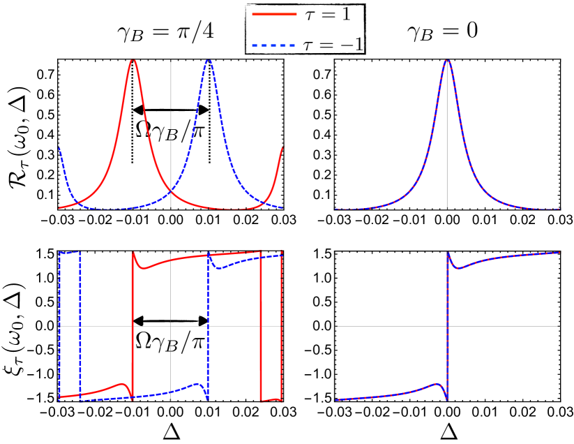
Figure 3: Reflection coefficient $R_{\tau}(\omega_{0},\Delta)$ (upper row) and the phase shift $\xi_{\tau}(\omega_{0},\Delta)$ (lower row) as a function of the detuning $\Delta=\Delta_{0}-\omega_{0}$ for the two parities $\tau=\pm 1$. In the left (right) columns we show the plots for $\gamma_{B}=\pi/4$ included (neglected), respectively. The red (full) and the blue (dashed) correspond to parity $\tau=1$ and $\tau=-1$, respectively. The position of the peaks shift between the two parities is $\Omega\gamma_{B}/\pi$. The values of the parameters are the same as in Fig. 2.

Typically, both the amplitude $T_{\tau}(\omega,\Omega)=|t_{\tau}(\omega,\Omega)|^{2}$ and the phase $\xi_{\tau}(\omega,\Omega)=\arctan[{\mathcal{I}m}(t_{\tau})/{\mathcal{R}e}(t_{\tau})]$ of the output signal are measured. In the main (inset) plot of Fig. 2 we show the reflection coefficient $R_{\tau}(\omega_{0},\Omega)=1-T_{\tau}(\omega_{0},\Omega)$ as a function of the driving frequency $\Omega$ for the two parities when we account for (neglect) the Berry phase contribution pertaining to the braiding of MBS. Moreover, we assume the cavity is probed at resonance $\omega=\omega_{0}$, and in this case we find the distance between the inverse of $n$-th order peaks of the two parities to satisfy

$$\gamma_{B}=\pi(\Delta_{0}-\omega_{0})\left(\frac{1}{\Omega_{n,-1}}-\frac{1}{\Omega_{n,+1}}\right)\,,$$ (15)

where $\Omega_{n,\tau}$ denotes the $n$-th resonance peak in the braiding frequency $\Omega$, for parity $\tau$. In an experiment, one can therefore extract the Berry phase associated with the braiding by measuring precisely this scaling from the transmission spectrum as a function of $\Omega$ when the cavity assists the braiding.

Similarly, to illustrate the versatility of our proposal, in Fig. 3 we plot $R_{\tau}(\omega_{0},\Delta)$ and the phase shift $\xi_{\tau}(\omega_{0},\Delta)$ as a function of the detuning parameter $\Delta$ in the presence (and absence) of the Berry phase $\gamma_{B}=\pi/4$. One can thus extract the Berry phase from the shift of the resonances for the two different parities from both quantities.

Conclusions.— We have studied the braiding of Majorana fermions in an Y junction geometry that is embedded in a microwave cavity. We have shown that both the parity of the ground state and the non-trivial Berry phase occurring during the braiding cycle imprint into the photonic field of the cavity that assists the process, which in turn can be probed non-invasively by the dispersive readout of the cavity microwave transmission. We found that these manifestations are purely dynamical, they occur in the absence of any splitting of the MBS that are exchanged, and they disappear in the static case. While here we focus on the effects of braiding on the photons, the reverse effect, namely the manipulation of braiding by means of the photonic field can be analyzed within the same framework.

Acknowledgments.— We would like to acknowledge discussions with Yipu Song, Kihwan Kim, Luyan Sun, and Yaroslav Tserkovnyak. MT acknowledges support from the National Basic Research Program of China Grants No. 2011CBA00300 and No. 2011CBA00302.

References

- Nayak et al. (2008) C. Nayak, S. H. Simon, A. Stern, M. Freedman, and S. Das Sarma, Rev. Mod. Phys. 80, 1083 (2008).
- Kitaev (2001) A. Y. Kitaev, Physics-Uspekhi 44, 131 (2001).
- Das Sarma et al. (2015) S. Das Sarma, M. Freedman, and C. Nayak, Npj Quantum Information 1, 15001 (2015).
- Aasen et al. (2016) D. Aasen, M. Hell, R. V. Mishmash, A. Higginbotham, J. Danon, M. Leijnse, T. S. Jespersen, J. A. Folk, C. M. Marcus, K. Flensberg, and J. Alicea, Phys. Rev. X 6, 031016 (2016).
- Alicea (2012) J. Alicea, Reports on Progress in Physics 75, 076501 (2012).
- Leijnse and Flensberg (2012) M. Leijnse and K. Flensberg, Semiconductor Science and Technology 27, 124003 (2012).
- Elliott and Franz (2015) S. R. Elliott and M. Franz, Rev. Mod. Phys. 87, 137 (2015).
- Aguado (2017) R. Aguado, Riv. Nuovo Cimento 40, 523 (2017).
- Lutchyn et al. (2010) R. M. Lutchyn, J. D. Sau, and S. Das Sarma, Phys. Rev. Lett. 105, 077001 (2010).
- Oreg et al. (2010) Y. Oreg, G. Refael, and F. von Oppen, Phys. Rev. Lett. 105, 177002 (2010).
- Mourik et al. (2012) V. Mourik, K. Zuo, S. M. Frolov, S. Plissard, E. Bakkers, and L. Kouwenhoven, Science 336, 1003 (2012).
- Deng et al. (2012) M. T. Deng, C. L. Yu, G. Y. Huang, M. Larsson, P. Caroff, and H. Q. Xu, Nano Letters 12, 6414 (2012).
- Das et al. (2012) A. Das, Y. Ronen, Y. Most, Y. Oreg, M. Heiblum, and H. Shtrikman, Nat. Phys. 8, 887 (2012).
- Churchill et al. (2013) H. O. H. Churchill, V. Fatemi, K. Grove-Rasmussen, M. T. Deng, P. Caroff, H. Q. Xu, and C. M. Marcus, Phys. Rev. B 87, 241401 (2013).
- Albrecht et al. (2016) S. Albrecht, A. Higginbotham, M. Madsen, F. Kuemmeth, T. Jespersen, J. Nygård, P. Krogstrup, and C. Marcus, Nature 531, 206 (2016).
- Deng et al. (2016) M. T. Deng, S. Vaitiekenas, E. B. Hansen, J. Danon, M. Leijnse, K. Flensberg, J. Nygård, P. Krogstrup, and C. M. Marcus, Science 354, 1557 (2016).
- Nichele et al. (2017) F. Nichele, A. C. C. Drachmann, A. M. Whiticar, E. C. T. O’Farrell, H. J. Suominen, A. Fornieri, T. Wang, G. C. Gardner, C. Thomas, A. T. Hatke, P. Krogstrup, M. J. Manfra, K. Flensberg, and C. M. Marcus, Phys. Rev. Lett. 119, 136803 (2017).
- Zhang and et al. (2018) H. Zhang and et al., Nature 556, 74 (2018).
- Lutchyn et al. (2018) R. M. Lutchyn, E. P. A. M. Bakkers, L. P. Kouwenhoven, P. Krogstrup, C. M. Marcus, and Y. Oreg, Nature Reviews Materials 3, 52 (2018).
- Liu et al. (2017) C.-X. Liu, J. D. Sau, T. D. Stanescu, and S. Das Sarma, Phys. Rev. B 96, 075161 (2017).
- Moore et al. (2018) C. Moore, C. Zeng, T. D. Stanescu, and S. Tewari, arXiv:1804.03164 (2018).
- Kitaev (2003) A. Y. Kitaev, Ann. Phys. 303, 2 (2003).
- Alicea et al. (2011) J. Alicea, Y. Oreg, G. Refael, F. von Oppen, and M. P. A. Fisher, Nat. Phys. 7, 412 (2011).
- Sau et al. (2011) J. D. Sau, D. J. Clarke, and S. Tewari, Phys. Rev. B 84, 094505 (2011).
- van Heck et al. (2012) B. van Heck, A. R. Akhmerov, F. Hassler, M. Burello, and C. W. J. Beenakker, New Journal of Physics 14, 035019 (2012).
- Pedrocchi and DiVincenzo (2015) F. L. Pedrocchi and D. P. DiVincenzo, Phys. Rev. Lett. 115, 120402 (2015).
- Pedrocchi et al. (2015) F. L. Pedrocchi, N. E. Bonesteel, and D. P. DiVincenzo, Phys. Rev. B 92, 115441 (2015).
- Knapp et al. (2016) C. Knapp, M. Zaletel, D. E. Liu, M. Cheng, P. Bonderson, and C. Nayak, Phys. Rev. X 6, 041003 (2016).
- Bauer et al. (2018) B. Bauer, T. Karzig, R. V. Mishmash, A. E. Antipov, and J. Alicea, SciPost Phys. 5, 004 (2018).
- Nag and Sau (2018) A. Nag and J. D. Sau, arXiv:1808.09939 (2018).
- Karzig et al. (2016) T. Karzig, Y. Oreg, G. Refael, and M. H. Freedman, Phys. Rev. X 6, 031019 (2016).
- Trif and Simon (2018) M. Trif and P. Simon, Supplementary Material (2018).
- Dmytruk et al. (2015) O. Dmytruk, M. Trif, and P. Simon, Phys. Rev. B 92, 245432 (2015).
- Dartiailh et al. (2017) M. C. Dartiailh, T. Kontos, B. Douçot, and A. Cottet, Phys. Rev. Lett. 118, 126803 (2017).
- Trif and Tserkovnyak (2012) M. Trif and Y. Tserkovnyak, Phys. Rev. Lett. 109, 257002 (2012).
- Goldin and Avishai (2000) Y. Goldin and Y. Avishai, Phys. Rev. B 61, 16750 (2000).
- Kohler (2017) S. Kohler, Phys. Rev. Lett. 119, 196802 (2017).