Novel Massive MIMO Channel Sounding Data applied to Deep Learning-based Indoor Positioning

Abstract

With a significant increase in area throughput, Massive MIMO has become an enabling technology for fifth generation (5G) wireless mobile communication systems. Although prototypes were built, an openly available dataset for channel impulse responses to verify assumptions, e.g. regarding channel sparsity, is not yet available. In this paper, we introduce a novel channel sounder architecture, capable of measuring multi-antenna and multi-subcarrier channel state information (CSI) at different frequency bands, antenna geometries and propagation environments. The channel sounder has been verified by evaluation of channel data from first measurements. Such datasets can be used to study various deep-learning (DL) techniques in different applications, e.g., for indoor user positioning in three dimensions, as is done in this paper. Not only we do achieve an accuracy better than $75\text{\,}\mathrm{cm}$ for line of sight (LoS), as is comparable to state-of-the-art conventional positioning techniques, but also obtain similar precision for the more challenging case of non-line of sight (NLoS). Further extensive indoor/outdoor measurement campaigns will provide a more comprehensive open CSI dataset, tagged with positions, for the scientific community to further test various algorithms.

I Introduction

An over-provisioning of antennas in Massive MIMO systems can be used to create orthogonal channels in space, resulting in higher area throughput [1]. Therefore, Massive MIMO has become an attractive preoposition for fifth generation (5G) wireless mobile communication systems [2, 3]. Although Massive MIMO prototypes were available as early as 2012 [4, 5, 6] and were showing promising results regarding the expected area throughput, an open source channel state information (CSI) database, tagged with GPS coordinates, including different frequency bands, antenna geometries and propagation environments to better evaluate the performance of Massive MIMO, is not yet available. Such publicly available datasets can be used for, e.g., testing precoding schemes with actual channel data, and to verify predictions on the achievable sum-rate. Thus, a novel channel sounder which is not limited to specific frequency bands or antenna geometries is needed for creating such database.

It is widely acknowledged in the research literature that Massive MIMO favors Time Division Duplexing (TDD) as mode of operation, owing to the fact that the piloting overhead is independent of the number of basestation antennas. This mode is also referred to as “canonical” Massive MIMO [1]. Still, industry strives for enabling Frequency Division Duplexing (FDD) Massive MIMO, as current network architectures favor FDD systems [7]. Thus, there is a significant body of papers assuming a (still to be verified) sparse channel model, leading to the possibility of using Joint Spatial Division and Multiplexing (JSDM) [8] and compressive sensing techniques [9]. By exploiting channel sparsity, different algorithms show the potential of achieving the same spectral efficiency as canonical (i.e., TDD-based) Massive MIMO [10]. However the question remains whether the measured channels in the lower frequency bands from 1 to $6\text{\,}\mathrm{GHz}$ exhibit the property of sparsity in real-world propagation environments. Due to the many antennas in Massive MIMO systems, measurement campaigns create a large amount of data, suggesting that machine learning and, in particular, DL techniques can be improved by making use of those datasets, e.g., for studying the unsolved task of indoor user localization [11, 12, 13, 14]: A Neural Network (NN) could exploit the large number of different channel estimates (per antenna and subcarrier) to predict the current position of the user. Just from considering these two possible applications, the need for a publicly available CSI position-tagged database becomes obvious.

In this paper, the main requirements for a channel sounder are shown and a novel low cost architecture for Massive MIMO measurements is proposed. Compare to the channel sounder proposed in [15] or any yet to be seen architecture, the proposed channel sounder reduces the number of analog to digital converter (ADC) per RF chain and therefore RF-topology complexity. The flexibility of the channel sounder regarding different frequency bands, antenna geometries and propagation scenarios is discussed. Also, sanity checks regarding viability, stability, hardware impairments and reproducibility of the channel sounding results are presented. As an application of the sounding data, initial results based on DL for indoor user positioning are shown, where an accuracy of better than $75\text{\,}\mathrm{cm}$ in three dimensions is achieved, indicating the potential of using Massive MIMO for indoor user positioning exploiting actual channel measurements.

II Channel Sounder Architecture

Let us first introduce the basic functionalities and requirements for the channel sounder is presented which is later used for verification of the proposed architecture.

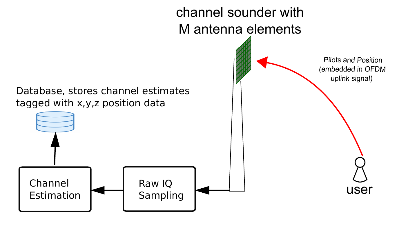
Figure 1: Massive MIMO channel sounder (CSI, user position)

Fig. 1 shows the system model of a channel sounder capable of capturing the CSI with the corresponding user position and storing it into a database. The procedure is as follows: The mobile user transmits OFDM signals containing pilots and the embedded user position; the signal is received at the channel sounder using an antenna array, and the raw I/Q-samples are stored for further post-processing. The complex channel coefficients per subcarrier and antenna are estimated offline and the position information is decoded from the payload, which is then saved into a database. To provide stable and consistent measurement datasets, the channel sounder needs to fulfill the following requirements regarding range, signal quality and reproducibility.

1. Requirement 1: Flexibility
   Different frequency bands result in different propagation behavior and, thus, a basestation could be able to chose the best frequency band for each scenario [16]. This leads to the requirement that the channel sounder should be capable of operating in different frequency bands in the sub-$6\text{\,}\mathrm{GHz}$ range. Moreover, different antenna geometries result in different channel estimation techniques as shown in [8]. Therefore, the channel sounder should be independent of the antenna array used, which, also, should be freely configurable.

2. Requirement 2: Coverage
   Coverage and, thus, keeping in mind the resulting path loss is key for each wireless communication system. LTE “suburban” was specified to achieve a coverage of around $5\text{\,}\mathrm{km}$, with a maximum path loss of $164.5\text{\,}\mathrm{dB}$ [16]. Since large parts of cellular systems are designed for a 1-2 km coverage radius, the requirement for the channel sounder should be to cover a similar range. Taking into account the well-known breakpoint model [16], a $110\text{\,}\mathrm{dB}$ pathloss with an SNR of at least $10\text{\,}\mathrm{dB}$ should still be achievable.

3. Requirement 3: Stability and reproducibility
   The last requirement is that each estimated channel should be the most precise representation of the physical channel possible. Hardware impairments should not unnecessarily limit the measurement accuracy, e.g., a small ADC resolution would lead to poor measurement accuracy. Moreover, the channel sounder should be stable over time and, thus, the channel must not change for a non-moving user, provided the propagation environment stays constant (e.g., indoor laboratory set-up).

Considering these requirements for obtaining an accurate CSI database, we designed a novel and low-cost channel sounder, as presented in the following.

II-A Principle of the channel sounder

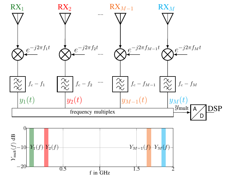
Figure 2: Basic principle of the channel sounder

Fig. 2 shows the basic principle of the novel channel sounder. Note that for simplification bandpass filter and amplifier for the analog front end (AFE) are omitted. Each antenna signal is mixed from the carrier frequency $f_{c}$ onto an individual intermediate frequency (IF) $f_{c}-f_{m}$, $m=1,..,M,$ to become $y_{m}(t)\;\laplace\;Y_{m}(f)$ and is then combined using a low-loss frequency addition (as detailed in the next section). Here the number of antennas is defined as $M$. The combined signal $Y_{\rm mult}(f)$ is fed to a single ADC with a high resolution and bandwidth. After analog to digital conversion the digital signal processing (DSP) unit splits the orthogonal frequency bands into single channels to estimate the CSI for each antenna separately (which can be done offline). As the discrete-time sampling is aligned in time among all antennas, a reduced number of calibration steps, e.g., no synchronization of multiple ADCs or calibrating multiple transit times, is needed. Although only the basic principle of receiver processing is shown, a transmitter (or even a full basestation) could be designed straightforwardly based on the same concept, simply by extending the AFE. Note that, only the AFE needs to be changed to work at different frequency bands; for example, our channel sounder is equipped for $1.25\text{\,}\mathrm{GHz}$, $2.35\text{\,}\mathrm{GHz}$ and $3.75\text{\,}\mathrm{GHz}$ operation.

Concerning Requirement 2, and the effect of using only a single ADC, the achievable signal-to-quantisation-noise-ratio (SQNR) per antenna is computed. A number of $N_{\text{Ant}}=64$ antennas, each having a bandwidth of $20\text{\,}\mathrm{MHz}$, are combined. The signal is then clipped with a clipping range of $U_{\text{VPP}}=$$100\text{\,}\mathrm{mV}$ and quantized with different effective number of bits (ENoB).

Figure 3: SQNR versus input Power at a 50Ohm input

Fig. 3 shows the simulated achievable SQNR versus the input power. One can see that, the communication quality dependens on the ENoB, as the subband signals are combined and each signal can only “consume” a fraction of the available ADC resolution. For measuring an $x,y$-plane in space, a constant clipping range is preferable to maintain the channels’ power relations.

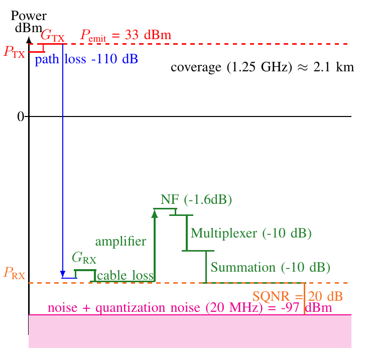
Figure 4: Link budget consideration

Fig. 4 shows the link budget consideration for this specific setup for one antenna chain. With an oscilloscope such as the LeCroy HD9404 [17] with 7.8 ENoB, and a targeted SNR of $20\text{\,}\mathrm{dB}$, the effective input power ranges from $-77\text{\,}\mathrm{d}\mathrm{B}\mathrm{m}$ to $-36\text{\,}\mathrm{d}\mathrm{B}\mathrm{m}$ for a bandwidth of $20\text{\,}\mathrm{MHz}$. With our setup ($G_{\text{RX}}=$3\text{\,}\mathrm{dB}$$,   $G_{\text{TX}}$=$3\text{\,}\mathrm{dB}$,   $P_{\text{TX}}$=$33\text{\,}\mathrm{dB}$,  $\text{Amp}_{\text{RX}}$=$20\text{\,}\mathrm{dB}$) and the breakpoint model assumption ($h_{\text{TX}}=h_{\text{RX}}=$1\text{\,}\mathrm{m}$$) the resulting maximum coverage radius (addressing Requirement 2) computes to

$$d_{\text{max}}=\left(\frac{\sqrt{h_{\text{TX}}h_{\text{RX}}}}{10^{-\text{PL}_{\text{BP}}/40}}\right)\approx$2.1\text{\,}\mathrm{km}$.$$ (1)

Moreover, we have decided to use an oscilloscope with 4 synchronized analog to digital converters (ADCs) and therefore the antennas are split onto 4 different channels, thus allowing to improve the SQNR per measurement chain. Note that the effect of clipping could be mitigated by an automated gain control (AGC) unit, however, at the cost of losing the individual channel power relations that make up the measured multiple antenna channel vector. As expected, a coarse gain adjustment, equal for all RX antenna chains, is still needed and indeed performed prior to each scenario measurement.

II-B Realization of the channel sounder

As the straightforward addition of antenna signals with Wilkinson combiners [18] would result in a loss of $3\log_{2}{\left(N_{\text{Ant}}\right)}$, a low-loss frequency multiplexing scheme is used. Due to size constraints and difficulties of matching many antennas on a printed circuit board (PCB), we have decided to place 10 antennas per PCB. For scaling to a higher number of antennas a production of the same PCB with the same filters and adjusting only the IF by programming the corresponding mixers is favorable. Therefore, a frequency-interleaved structure of combining PCBs is used, resulting in 10 subbands (sb.) as shown in Fig. 5.

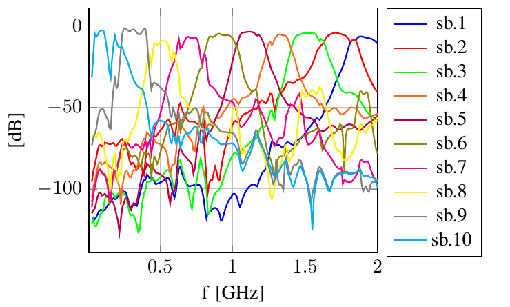
Figure 5: Transfer functions of the multiplexing scheme

Fig. 5 indicates (simulation) that the subbands are separated by more than 20dB and, therefore, mutual cross-correlations should be sufficiently suppressed. Note that, in the example given, 4 antennas (4 PCBs) are placed within one subband.

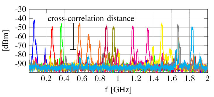
Figure 6: Measured cross-correlation power among subbands

Fig. 6 shows, for one specific (yet typical) example that the measured channels (and individual subbands) are decoupled with at least 30dB. Therefore, any cross-correlation showing up using this architecture can be neglected in the following.

Figure 7: Channel sounder (daughterboards) with digital oscilloscope and antenna array

Fig. 7 shows the receiver part of the channel sounder with 64 antennas. The signal is received over the modular (dual polarized) array and then filtered, amplified, mixed (down-converted) and combined within so called “daughterboards”. Then, two daughterboards with different frequency settings are combined onto one port of the oscilloscope. The signal is then mixed to baseband (offline, in digital signal processing), filtered, resampled and, finally, the channel coefficients are estimated. Note that the clock of an external source is fed to the oscilloscope and to all of the mixers on the daughterboards, resulting in a frequency aligned receiver.

The transmitter consists of a USRP [19], an amplification circuit and a dipole antenna, which transmits orthogonal frequency division multiplex (OFDM) symbols with a bandwidth of $20\text{\,}\mathrm{MHz}$, and 1024 subcarriers as pilots and data on the HAM radio frequency of $1.25\text{\,}\mathrm{GHz}$. Note that 10% of the subcarriers are used as a guard band and the cyclic prefix was 1/8 of the OFDM symbol duration. For subcarrier modulation, a simple QPSK constellation was chosen.

III Verification of the Channel Sounder

To satisfy Requirement 3, different stability and hardware impairment criteria are studied via test measurements. First, two fixed positions are measured to verify the stability of the channel sounder. Later, different indoor scenarios were chosen for generating a data set to evaluate user positioning algorithms based on deep learning.

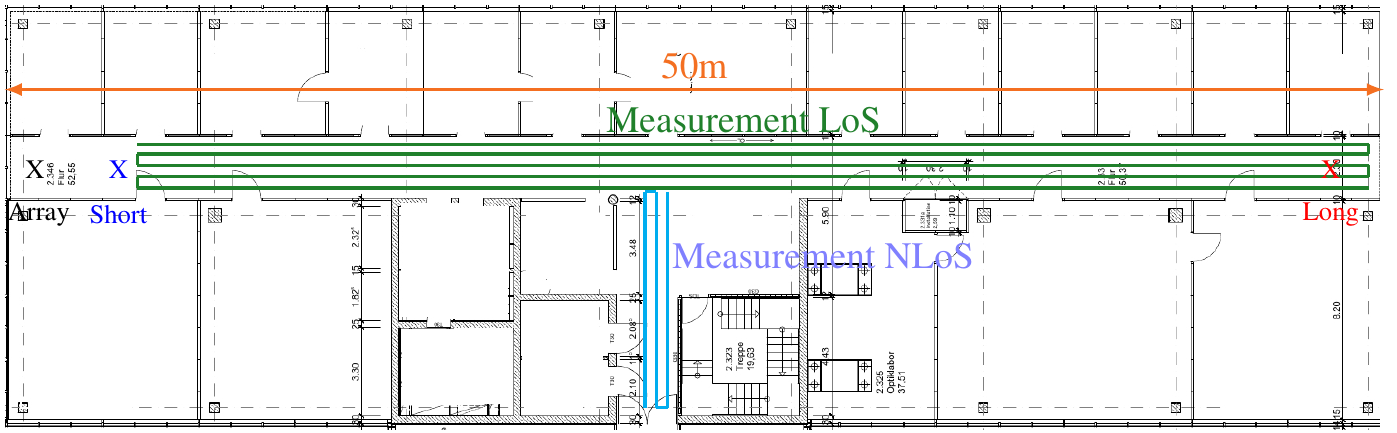
Figure 8: Indoor measurement scenario (office space with hallway)

Fig. 8 shows the different indoor measurement scenarios where the array is configured as an 8x8 horizontally polarized rectangular array. First, two stable positions “Short” and “Long” are measured for stability study. Later, the LoS and NLoS paths are measured at 3 different heights above the floor (0.5m, 1m, 1.5m), resulting in about $600\text{\,}\mathrm{m}$ and $200\text{\,}\mathrm{m}$ total measurement path length for LoS and NLoS, respectively. As references for positioning, every $2\text{\,}\mathrm{m}$ a grid point was marked on the floor, and positions were interpolated within. It was verified that the resolution of this “position ground truth” is better than 10cm.

III-A Stability

For the stability over time the correlation coefficient

$$\delta_{h}\left(\Delta t\right)=\frac{1}{N_{\text{Sub}}}\sum_{k=0}^{N_{\text{Sub}}}\frac{\left\|{\textbf{h}(k)}_{t}{\textbf{h}(k)}_{t+\Delta t}^{H}\right\|_{2}}{\left\|{\textbf{h}(k)}_{t}\right\|_{2}\left\|{\textbf{h}(k)}_{t+\Delta t}\right\|_{2}},$$ (2)

of the $64\times 1$ complex channel vector $\textbf{h}(k)$ is evaluated. The correlation coefficient is averaged over all subcarriers $k$. Moreover, the signal-to-noise-ratio (SNR) of each antenna is calculated over the error vector magnitude (EVM).

Figure 9: Verifying amplitude/phase stability

Fig. 9 shows the correlation coefficient over time for the different measurements “Short” , “Long” and “Moving”, and plots the cumulative distribution function (CDF) of all measured SNRs. It can be seen that the SNR always stays above $10\text{\,}\mathrm{dB}$ for every antenna and, on average is about $25\text{\,}\mathrm{dB}$. Therefore, the signal quality over the 10 minute measurement is good enough to verify stability. With an average correlation coefficient above 0.8 over 10 min, the measurement setup can be considered to be sufficiently stable. To cross-check, when moving the transmitter, the correlation coefficient falls well below 0.5, which is a plausible observation.

III-B Sanity checks for hardware impairments

For a transmission scheme with one transmitter and 64 receive antennas, the received signal can be written [1] as

$$\bf{y}_{\it{k}}=\bf{w}_{\it{k}}^{H}\bf{h}_{\it{k}}s_{\it{k}}+\bf{w}_{\it{k}}\bf{n}_{\it{k}},$$ (3)

where $\bf{w}_{\it{k}}$ is the $1\times 64$ linear combining vector, $\bf{h}_{\it{k}}$ is the $64\times 1$ channel vector, $s_{\it{k}}$ is the transmitted QPSK symbol and $\bf{n}_{\it{k}}$ is the $64\times 1$ additive white Gaussian noise vector for each subcarrier $k$. To verify whether the hardware impairments are limiting the gain of the linear combining scheme, a simple maximum ratio combining (MRC) scheme is investigated, where the combining vector

$$\bf{w}_{\it{k}}=\bf{\hat{h}}_{\it{k}},$$ (4)

is used and where $\bf{\hat{h}_{\it{k}}}$ is the estimated channel vector. In a non-hardware limited system and with equal SNR per antenna, a 3dB gain in the bit error rate (BER) curve per doubling of the number of antennas would be expected.

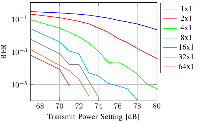
Figure 10: Measured MRC gain vs number of RX antennas

Fig. 10 shows the BER curves for different number of antennas, when the transmitter gain of the TX-USRP is sweeped. Hereby QPSK symbols were transmitted and the BER of a channel were measured after combining. Note that all 64 antennas were measured and the “virtual” antennas to combine were chosen as follows: An antenna with a moderate to low SNR was chosen as the first BER curve and then the antenna with the next higher SNR was used for MRC, and so on. With the difference in SNR a gain higher than $3\text{\,}\mathrm{dB}$ can occur, as can be seen in the figure (channel is not ideal AWGN). Moreover, the expected gains of MRC appear and verify that the hardware impairments constrain our system only very little (even though the gain from 32 antennas to 64 antennas is not quite 3 dB, indicating the presence hardware impairments), verifying the usability of the channel sounder.

IV First Trials for Indoor 3D-User Positioning

One first example for showing the potential of position-tagged CSI dataset is shown next, for the case of the yet unsolved problem of indoor user positioning [12]. The two paths (LoS and NLoS) shown in Fig. 8 are measured at 3 different heights ($0.5\text{\,}\mathrm{m}$, $1\text{\,}\mathrm{m}$, $1.5\text{\,}\mathrm{m}$) above the floor. Each time a position-tagged dataset of about 2000 spatial points per height is created, resulting in an average distance per point of $\lambda/2$.

TABLE I: Layout of the neural net for 64 antennas

Layers:	Output dimensions
Input	64 x 922 x 2 (Re/Im)
Conv2D	64 x 922 x 32
AveragePooling	64 x 231 x 32
Conv2D	64 x 231 x 32
AveragePooling	64 x 58 x 32
Dense	256
Dense	256
Dense	256
Dense	3 (X/Y/Z)

An NN (example given for 64 antennas in Table I) is trained, based on the measured channels from all antennas and on all sub-carriers, to estimate the position. For this, 90 % percent of the data was used for training and 10 % for validation. Note that the NN has a number of weights ranging from $\approx 1,000,000$ to $\approx 16,000,000$. This is due to the fact that for a fair comparison the net structure is the same when going from 2 to 64 antennas, but the input dimension increases. The convolutional layers were chosen according to the rationale that always 4 subcarriers are assumed to be correlated. This information is averaged for condensing the data without losing information.

IV-A Line-of-Sight Positioning

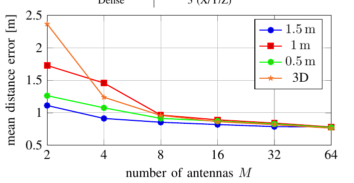
Figure 11: Measured position error, indoor LoS scenario

Fig. 11 shows the mean distance error between the actual position $\mathbf{d}$ and the expected position $\hat{\mathbf{d}}$ over the number of antennas. As can be seen, when going from 2D to 3D user localization a difference only occurs for the region of small number of antennas. A positioning precision of about $75\text{\,}\mathrm{cm}$ is achieved over the entire measurement area, outperforming other state-of-the-art methods [12]. To better understand the further possible improvements, the histogram of the positioning error is further examined.

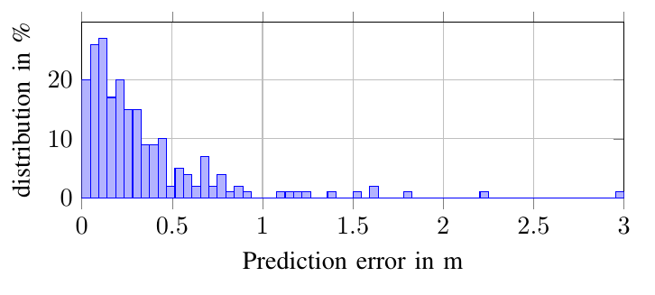
Figure 12: Distribution of distance error

Fig. 12 shows the histogram of the prediction error which follows a Rayleigh-like distribution, as the $x,y,z$ error seems to be Gaussian distributed. Moreover, there are positions having an error of meters, which were located at sharp edges nearby doors. For the LoS case, passive radar systems would also be a possible solution, but in the more sophisticated case of NLoS they do not work. This is the reason why we move on to studying the NLoS region more closely.

IV-B Non-Line-of-Sight Positioning

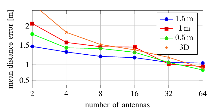
Figure 13: Measured positioning error, indoor NLoS scenario

Fig. 13 shows the positioning error over the number of receive antennas. The prediction error increases to  $95\text{\,}\mathrm{cm}$, which is due to both the NLoS environment as well as the further distance from the antenna array. Still, the system predicts the user positions remarkably well. It appears that DL in combination with Massive MIMO datasets has the potential of addressing the task of indoor user localization with better prediction accuracy than other known methods thus far.

V Outlook and Conclusion

We introduce a channel sounder that enables the generation of a publicly available position-tagged Massive MIMO database, in support of better evaluating channel properties as well as studying deep learning techniques on measured channel data. The main requirements regarding stability, flexibility and coverage for a channel sounder where shown. A novel channel sounder architecture is proposed to meet those requirements, and its viability is verified via simulation as well as actual measurements. Using this channel sounding data, initial results for 3D-indoor user positioning via deep learning have been obtained, beating state of the art systems, even in the more difficult scenario of NLoS. Further work will address different frequency bands, other antenna geometries and propagation scenarios. In the near future and enriched with new measurements a database will be made public for the scientific community to test-run their own algorithms for various applications, beyond precoding and user positioning.

References

- [1] E. Björnson, J. Hoydis, and L. Sanguinetti, “Massive MIMO networks: Spectral, energy, and hardware efficiency,” Foundations and Trends in Signal Processing, 2017.
- [2] F. Boccardi, R. W. Heath, A. Lozano, T. L. Marzetta, and P. Popovski, “Five disruptive technology directions for 5G,” IEEE Communications Magazine, 2014.
- [3] E. G. Larsson, O. Edfors, F. Tufvesson, and T. L. Marzetta, “Massive MIMO for next generation wireless systems,” IEEE Communications Magazine, 2014.
- [4] X. Xie, E. Chai, X. Zhang, K. Sundaresan, M. A. Khojastepour, and S. Rangarajan, “Hekaton: Efficient and practical large-scale mimo,” 2015.
- [5] C. Shepard, H. Yu, N. Anand, E. L. Li, T. L. Marzetta, Y. R. Yang, and L. Zhong, “Argos: practical many-antenna base stations,” 2012.
- [6] S. Malkowsky, J. Vieira, L. Liu, P. Harris, K. Nieman, N. Kundargi, I. Wong, F. Tufvesson, V. Owall, and O. Edfors, “The World’s First Real-Time Testbed for Massive MIMO: Design, Implementation, and Validation,” IEEE Access, 2017.
- [7] E. Björnson, E. G. Larsson, and T. L. Marzetta, “Massive MIMO: Ten Myths and One Critical Question,” IEEE Communications Magazine, vol. 54, no. 2, pp. 114–123, February 2016.
- [8] J. Nam, J. Ahn, A. Adhikary, and G. Caire, “Joint spatial division and multiplexing: Realizing massive MIMO gains with limited channel state information,” March 2012, pp. 1–6.
- [9] Z. Gao, L. Dai, S. Han, C. I, Z. Wang, and L. Hanzo, “Compressive sensing techniques for next-generation wireless communications,” 2018.
- [10] Z. Jiang, A. F. Molisch, G. Caire, and Z. Niu, “On the achievable rates of fdd massive mimo systems with spatial channel correlation,” Oct 2014, pp. 276–280.
- [11] M. Arnold, S. Dörner, S. Cammerer, and S. ten Brink, “On Deep Learning-based Massive MIMO Indoor User Localization,” 2018.
- [12] D. Lymberopoulos, “Microsoft Indoor Localization Competition – IPSN 2018,” Microsoft, Tech. Rep., 2018.
- [13] Alexis Decurninge and Luis Garcia Ordóñez and Paul Ferrand and Gaoning He and Bojie Li and Zhang Wei and Maxime Guillaud, “CSI-based Outdoor Localization for Massive MIMO: Experiments with a Learning Approach,” 2018.
- [14] J. Vieira, E. Leitinger, M. Sarajlic, X. Li, and F. Tufvesson, “Deep convolutional neural networks for massive MIMO fingerprint-based positioning,” 2017.
- [15] Nielsen, Jesper and Fan, Wei and C F Eggers, Patrick and Pedersen, G.F., “A Channel Sounder for Massive MIMO and mmWave Channels,” IEEE Communications Magazine, 08 2018.
- [16] 3GPP, “Technical Specification Group Radio Access Network,” 3GPP, Tech. Rep., 2012.
- [17] Teledyne LeCroy HDO9404. [Online]. Available: https://www.teledynelecroy.com
- [18] E. J. Wilkinson, “An N-Way Hybrid Power Divider,” IRE Transactions on Microwave Theory and Techniques, 1960.
- [19] B210 and B200. [Online]. Available: https://www.ettus.com/