Efficient Hotspot Switching in Plasmonic Nanoantennas using Phase-shaped Laser Pulses controlled by Neural Networks

Alberto Comin^∗ and Achim Hartschuh

Department of Chemistry and Center for NanoScience (CeNS), LMU Munich, 81377, Munich, Germany

^∗alberto.comin@cup.uni-muenchen.de

Abstract:   We present a novel procedure for manipulating the near-field of plasmonic nanoantennas using neural network-controlled laser pulse-shaping. As model systems we numerically studied the spatial distribution of the second harmonic response of L-shaped nanoantennas illuminated by broadband laser pulses. We first show that a trained neural network can be used to predict the relative intensity of the second-harmonic hotspots of the nanoantenna for a given spectral phase and that it can be employed to deterministically switch individual hotspots on and off on sub-diffraction length scale by shaping the spectral phase of the laser pulse. We then demonstrate that a neural network trained on a $90~{}\mathrm{nm}\times 150~{}\mathrm{nm}$ nano-L can in addition efficiently predict the hotspot intensities in an antenna with different aspect ratio after minimal further training for varying spectral phases. These results could lead to novel applications of machine-learning and optical control to nanoantennas and nanophotonics components.

OCIS codes: 190.7110 Ultrafast nonlinear optics, 250.5403 Plasmonics

1 Introduction

Plasmonic nanoantennas can efficiently focus broadband optical fields to form nanometer sized ultrafast hotspots [1, 2]. They could thus become a key component of future nanophotonic devices, combining high storage density and fast processing of information [3, 4, 5, 6]. The ability to deterministically control the brightness of individual hotspots within a nanoantenna by varying the input optical fields would add enormous flexibility to antenna schemes. Towards this goal, several groups have explored the possibility of controlling the near-field in plasmonic structures by tuning the spectrum, polarization and spectral phase profile of the input laser excitation [7, 8, 3, 9, 10, 11].

Spectral amplitude shaping could be applied in the simple case in which the nanoantenna features spectrally distinct plasmonic resonances connected to hotspots at different positions. For such nanoantennas, it is possible to lit each hotspot individually by tuning the color of the excitation light, albeit at the expense of reduced spectral bandwidth and thus temporal resolution. In more general cases, spatio-temporal control of plasmonic near-fields is understood to have two main control mechanisms [7]. Efficient tuning can be achieved by polarization pulse shaping which exploits the interference of plasmonic near-field modes with different polarization responses. Polarization pulse shaping has wide applicability and was successfully used to experimentally demonstrate sub-wavelength hotspot switching on different antenna systems [12, 7]. The second control mechanism is based on spectral phase shaping without the need of polarization control. In this scheme, the spatial control of non-linear responses is achieved by imprinting a spectral phase profile on the incident laser pulses which is set to compensate the phase response of the nanoantenna at a particular position [10, 13, 14].

Whereas for simple systems the parameters for the coherent control of the hotspot position can mostly be derived analytically, the optimum pulse characteristics for more complex multi-modal systems cannot be predicted [15]. Although evolutionary algorithms, such as genetic algorithms (GA), could be employed as versatile optimization tools for such problem sets, they typically require a large number of experimental iterations and are thus limited in efficiency [16]. Furthermore, the results obtained by GA are hard to generalize and replicate, while the GA must be re-optimized for each sample and experimental configuration. For example, when an external perturbation shifts the plasmonic resonance of the nanoantenna, the GA can only adapt by crossover and random mutation, without taking into account previously learned information about the sample [17].

We propose a combined use of GA and neural-network (NN) as a more efficient and deterministic way to control the near-field in plasmonic nanoantennas. NN have a layered structured which can encode more general information in the first layers and more specific information in the last layers [18]. This is one of the main reasons why NNs became very popular: It is possible to re-use a pre-trained NN on a different domain after just minimal training of the final layers [18].

In the following, we will show that a NN consisting of only four fully connected layers can accurately encode the dependence of the near-field on the spectral phase of the incident laser pulses.  [10, 13, 14]. Moreover, a NN trained on a specific nanoantenna can also be used with minimal further training on nanoantennas with different size and aspect ratio.

As an example of the efficacy of this approach, we apply the GA-NN combination to achieve second harmonic generation (SH) hotspot switching in L-shaped plasmonic nanoantennas by means of spectral-phase shaping. L-shaped nanoantennas were selected as simple model systems supporting multiple plasmonic resonances within the spectrum of ultrafast Ti:Sapphire lasers. Whereas polarization pulse shaping could be exploited as an additional powerful degree of freedom, here we wanted to limit the complexity of the optimization scheme. Although sub-wavelength and second-harmonic hotspot switching have been separately demonstrated [12, 10], the control of SHG in sub-diffraction nanoantennas was not shown before.

2 Setup

In order to use NNs for optimal control on real nanoantennas, a reasonable feasibility step is to train them using realistic simulated data. Producing high-quality nanostructures and measuring them is still a time-consuming task, but a vast simulated dataset can be produced in much shorter time. Plasmonic nanostructures are particularly convenient to simulate: Their optical properties are dominated by the surface density of charge and current, and it is possible to accurately model them using a boundary element method (BEM) [19]. For this purpose we applied a customized version of the Matlab MNPBEM toolbox [20], which was extended to perform non-linear optics simulations: additional details are provided in the appendix in section 5.2.

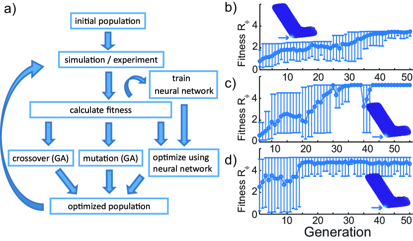
Fig. 1: a) Flow diagram of the training phase of the neural network using the population generated by a genetic algorithm. A random initial population of 20 spectral phases is chosen. At each iteration, the fitness is calculated according to a pre-specified goal: The fittest individuals are kept unchanged and the rest undergo mutation or cross-over. The least fit individuals are optimized by the NN using back-propagation. b) Training history of the GA without assistance from the NN. The graph reports the fitness of the best and worst individuals, and the average fitness. The fitness function (vertical axis) was chosen to maximize the relative SHG flux at a target hotspot of a $90~{}\mathrm{nm}\times 250~{}\mathrm{nm}$ gold L-shaped nanoantenna, indicated by an arrow in the inset. c) Similar to b) but with the GA assisted by an un-trained NN. d) similar to b) but with the GA assisted by a pre-trained NN: The fitness of the best individuals converges after just one iteration, the fitness of the worst individual remains lower due to the random mutations introduced by the GA.

We trained the NN using the populations produced by a genetic algorithm, as illustrated in Figure 1a. Using a GA has a double advantage: First, it allows to have a fast feedback on the nanoantenna design, e.g. if it is likely or not to be controllable withing the given experimental parameters. Second, it generates a varied dataset of both near-optimal and pseudo-random solutions. At each iteration the population was used to train the NN and then sub-divided according to the relative fitness: a few of the fittest individuals were kept unchanged, 80% of the remaining fittest were used to create crossover children and the rest underwent random mutation. The least fit individuals were optimized by the NN using a back-propagation algorithm [21]. The choice of optimizing the least fit individuals allows the possibility to start with an untrained NN. As the NN was trained, its accuracy increased until it started to accelerate the training of the GA. When the NN was sufficiently trained, it could be directly used to produce optimal solutions.

We note that an alternative and simpler way to generate a set of training spectral phases would be to use a random numbers generator. However, random phases tend to have fast oscillations that increase the pulse duration and reduce any nonlinearity.

For the results in this paper, the NN was trained to predict the second-harmonic (SH) flux at the hotspots on the surface of the nanoantenna utilizing the spectral phase of the laser excitation pulse as input. For efficiency reasons, the spectral phase was specified at 6 nodal points, evenly distributed within 2 standard deviations from the central frequency of the laser excitation pulse. The phases were then interpolated on a finer mesh, using piecewise cubic Hermite interpolation (pchip). An advantage of this approach is that it produces reasonably smooth phase profiles, without fast oscillations. The spectral phase at the nodal points was bounded between $\pm 100~{}\mathrm{rad}$, an interval chosen to match the capability of a standard $128~{}\mathrm{pixel}$ pulse-shaper. The spectral amplitude was taken to be Gaussian with central frequency of $375~{}\mathrm{THz}$ ($800~{}\mathrm{nm}$) and standard deviation of $26.5~{}\mathrm{THz}$, corresponding to a full-width-half-max (FWHM) temporal intensity duration of $10~{}\mathrm{fs}$. These constrains will make the results easier to test in an experimental setup equipped with a pulse-shaper and a femtosecond laser source.

3 Results and Discussion

The efficacy of the NN to accelerate the training of a GA is demonstrated in Figure 1. Panel b) shows the convergence of the GA without assistance of the NN for a $90~{}\mathrm{nm}\times 250~{}\mathrm{nm}$ L-shaped gold nanoantenna. The bars indicate the fitness of the best and worst individuals and the average fitness. The fitness function was chosen to maximize the relative SH flux at a specific hotspot, indicated in the inset by an arrow: $R_{\phi}=h_{\phi,i}/\underset{i\neq j}{\max}(h_{\phi,j})$, where $R_{\phi}$ is the fitness, $h_{\phi,i}$ is the SH flux at the target hotspot ’$i$’ resulting from a specific spectral phase profile $\phi$ and $\underset{i\neq j}{\max}(h_{\phi,j})$ is the maximum SH flux using the same phase $\phi$ over all the other hotspots. The inset shows the generated distribution of the SH field at the outer surface of the nanoantenna for a flat phase pulse. Figure 1c,d shows that a un-trained neural network can reduce the number of needed iterations substantially and that, with a pre-trained NN, the fitness of the best individual converges to the optimal value in just one iteration.

Optimizing the relative local intensity of the SH allows to switch the position of the brightest hotspot.

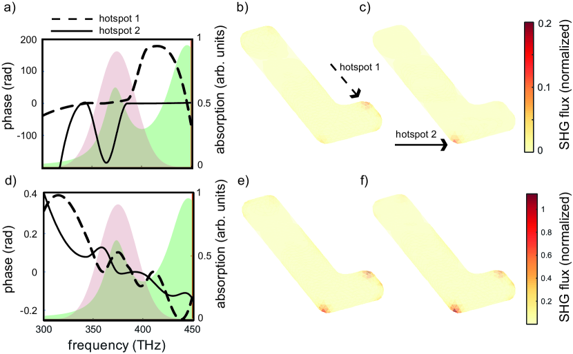
Fig. 2: Hotspot switching in a $90~{}\mathrm{nm}\times 250~{}\mathrm{nm}$ gold nanoantenna. a) Spectral phases which maximize the relative flux intensity of two hotspots (labeled ’1’ and ’2’) as found by the GA+NN algorithm. The hotspot positions are indicated by arrows in panels b,c). The laser spectrum (orange shaded area) and the nanoantenna absorption spectrum (green shaded area) are also shown. b,c) SHG flux intensity at the outer surface of the nano-antenna corresponding to the optimal phases shown in panel a). Panels d,e,f) report similar information as panels a,b,c) but with a different optimization goal: to maximize the absolute, rather than the relative, SH flux intensity at a specific hotspot

The idea of hotspot switching is illustrated in Figure 2. Panel a) shows the laser spectrum, the nanoantenna absorption spectrum and the spectral phases which maximize the relative SH flux $R_{\phi}$ as defined above at the hotspots labeled ’1’ and ’2’ in b) and c), respectively. Panel b) shows the SH surface field: It can be recognized that the location $x$ of the brightest hotspot changes according to the optimization goal $F_{\phi}(x)$. The color scale was normalized to the maximum SH surface flux for a flat phase laser pulse. It can be recognized that maximizing the relative intensity of a specific hotspot comes with a reduction of the overall SHG flux intensity of a factor of five.

Whilst optimizing the relative hotspot intensity is interesting, it result in a overall decrease of the SH intensity, which might be detrimental for actual applications. A different optimization goal is to maximize the absolute value of the SH flux for a given hotspot. The fitness is now defined by $A_{\phi}=h_{\phi}/h_{0}$, where $h_{\phi}$ is again the SH flux at the target hotspot resulting from a specific spectral phase $\phi$ and $h_{0}$ is the SH flux over all the nanoantenna surface for a flat spectral phase profile. In this case we are not guaranteed that the target hotspot will be the brightest one, but the resulting local fields will be larger.

We present the results of this kind of optimization in Figure 2d,e,f. For the a 90 nm250 nm gold nanoantenna the intensity gain was about a factor of 5 as compared to the optimization in Figure 3b, c as can be seen from the respective color bars.

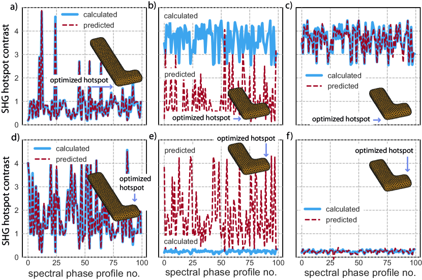
Fig. 3: a) Relative SH flux intensity for a target hotspot of a gold L-shaped nanoantenna with size $90~{}\mathrm{nm}\times 250~{}\mathrm{nm}$ for different spectral phase profiles of the incident laser pulse. The blue line refers to the simulated value, the red dashed line refers to the value predicted by the NN. The inset shows the nanoantenna with target hotspots marked. Panel b,c) shows the performance of same NN but used to predict the SHG hotspot intensities for a nanoantenna with different size: $90~{}\mathrm{nm}\times 150~{}\mathrm{nm}$ with no further training, and after training only the output layer of the NN for 10 epochs. d,e,f) report similar results as a,b,c) but for a different hotspot. The figure illustrates the flexibility of the NN with respect to the sample size and aspect ratio.

The results shown in Figure 3 demonstrate the possibility of switching the position of the main hotspot between different corners of an L-shaped nanoantennas. The displacement distance, for the illustrated case, was $100~{}\mathrm{nm}$, well below the diffraction limit for the laser excitation at $800~{}\mathrm{nm}$. The maximum contrast values, integrated over the whole frequency range, were: $R_{\phi}=5.2$ and $R_{\phi}=4.6$, for the two shown hotspots, which should be large enough to be experimentally tested. Such hotspot switching could be useful for triggering local non-linear phenomena, either in a adjacent sample object, such as a fluorescent molecule or semiconductor nanocrystal or, more simply, in the substrate of the nanoantenna

Analyzing the spectral phase profiles found by NN-GA combination in Figure 2a) and d) for the two different fitness functions $R_{\phi}$ and $A_{\phi}$, we can comment on the mechanisms underlying hotspot control in the present system. In case of the optimization of the relative flux $R_{\phi}$ at hotspot ’1’, the phase profile $\phi$ remains essentially flat between 320 and 390 THz, the spectral range of the plasmon resonance connected to this particular hotspot. From 395 to 450 THz, on the other hand, the phase becomes very large featuring huge higher order variations. This leads to an efficient suppression of the SH flux of the plasmon mode in this spectral range, which is associated with a different hotspot distribution including a peak at position ’2’. Optimizing the relative flux at hotspot ’2’ is seen to result in the opposite spectral phase characteristics with a flat curve between 450 to 395 THz and strong phase variations below.

For the target function $A_{\phi}$, which maximizes the absolute SH flux at a given hotspot position, the observed phase variations are much smaller. Here, the dominant control mechanism will be that of local pulse compression, also mentioned in the introduction [10, 13, 14]. In other words, the optimum spectral phase profiles found by the NN+GA scheme will compensate the local phase response of the nanoantenna at the particular positions thereby maximizing the non-linear response.

An important advantage of NN-based control is expected to arise from the adaptability of a trained network to similar problem sets. Applied to coherent control of plasmonic nanoantennas, this means that we could train our NN on a specific nanoantenna and then use the learned weights also for nanoantennas with different sizes or aspect ratios. The feasibility of this idea is demonstrated in Figure 3. Panel a) shows the prediction accuracy of a pre-trained NN for a set of randomly generated spectral phases and for a nanoantenna of size $90~{}\mathrm{nm}\times 250~{}\mathrm{nm}$, using a training set of $800.000$ phases, a test set of $90.000$ phases and $1000$ epochs. The blue line refers to the true value for the relative intensity of a target hotspot, marked with an arrow in the inset of panel c). The red line shows the prediction by the NN. The overall root square error was about $2.6\times 10^{-2}$. Panel b) shows the performance of the same NN but for a nanoantenna with size $90~{}\mathrm{nm}\times 150~{}\mathrm{nm}$, and panel c) after fine tuning only the last layer of the NN for $10$ epochs. The root mean square error was $0.98$ with no training and $5.7\times 10^{-2}$ after fine tuning. The NN was still able to quite accurately predict the relative intensity of the SH hotspot. Panels d,e,f) report similar results, but for a different hotspot, which was bright of the training antenna and dim on the test one: also in this case the NN was able to make quite accurate predictions, with a relative error of about $10$%.

These results indicate that it should be feasible to use a NN trained with simulated data to control a real nanoantenna in an experimental setup. Due to small changes in the dielectric environment and uncertainties in the fabrication process, the plasmon frequencies could be different between the real and the simulated nanoantennas. The ability of the NN to compensate for the frequency shifts caused by changes in size and aspect ratio suggests that the they could also adapt to shifts caused by the dielectric environment.

4 Conclusion

We introduced a novel scheme to control the near-field of plasmonic nanostructures based on a neural network in conjunction with a genetic algorithm. The neural network accelerates the optimization of the genetic algorithm and stores information about the sample, which can readily be generalized to other samples, with none or minimal further training. In order to prove the efficacy of this approach, we showed how the algorithms can find the optimal spectral phases for switching the position of the brightest hotspot in an L-shaped gold nanoantenna. We also showed that a NN trained on a specific nanoantenna provides quite accurate results also for a nanoantenna with different size and aspect ratio, even without any further training. Our results suggests that NNs are a powerful tool for optimal control of near-fields at the nanoscale and, in perspective, for more complex nanoplasmonics and nanophotonics devices. Coherent control of hotspot positions on the nanoscale could be experimentally observed using photoemission electron microscopy (PEEM) or scanning near-field optical microscopy with passive probes [12, 22]. Possible further developments include the coupling of nanoantennas to different emitters or waveguides situated near the hotspots providing a means for all-optical ultrafast switching or the spatially selective initiation of photochemical reactions at plasmonic nanoantennas [23].

5 Appendix

5.1 Neural Network

The neural-network (NN) used to obtain the results shown in the article was a multi-layer perceptron composed of four fully-connected layers, plus an input and an output layer. The activation function was hyperbolic tangent (tanh) for all layers except for the output layer, which had linear activation. The input layer contained 6 neurons representing the spectral phase of the excitation laser at 6 equidistant nodal points evenly distributed within 2 standard deviations from the central frequency of the laser excitation pulse. The phases were then interpolated on a finer mesh, using piecewise cubic Hermite interpolation (pchip). The sizes of the inner layers were: 100, 100, 50, 50. The output layer was used to predict the second-harmonic flux intensity for the 12 corners of a L-shaped nanoantenna.

The number of layers and neurons was chosen as a trade off between prediction accuracy and training speed. A small network requires a relatively small training dataset, and it can potentially be trained using experimental data within a reasonable measurement time. The network was trained using a custom implementation of the back-propagation algorithm in Matlab. The language was chosen for easier integration with existing toolboxes for optics and plasmonics. The accuracy of the code was tested using a widely-used machine-learning toolbox (Keras2 with TensorFlow back-end). The NN was trained using using the population generated by a genetic algorithm (GA). Several training sessions were run while changing optimization goals, e.g. relative or absolute hotpot intensity for different choices of hotspots. The final train set size was about 1 million, and the test set size about 0.1 million. A small ($10^{-6}$) $L_{2}$ regularization factor was used, however the regularization choice was not crucial when training the NN using noiseless simulated data: It will be important for training using real experimental data.

5.2 SHG Simulations

The second-harmonic response of the L-shaped nanoantennas was calculated using the boundary-element method, as described by Garcia de Abajo et al. [24]. An open-source Matlab toolbox (MNPBEM) was used to calculate the linear response of the nanoantennas [20]. The surface density of charge and current was than used to estimate the dipolar contributions to the SHG from each surface elements [25, 26]. For simplicity, the bulk contribution to the SHG was not considered. The simulation was performed in frequency domain using 200 points between $200~{}nm$ and $1000~{}nm$, the results were then interpolated using a finer mesh over the spectral range of the laser excitation. The simulated laser pulse was a Gaussian with temporal full-width-half-maximum width of $10~{}\mathrm{fs}$ and central frequency of $375~{}\mathrm{THz}$ ($800~{}\mathrm{nm}$).

6 Funding Information

Deutsche Forschungsgemeinschaft (DFG) HA4405/8-1

7 Acknowledgments

The authors thanks Giovanni Piredda, Nicolas Coca Lopez, Veit Giegold and Richard Ciesielski for helpful discussions.