Optimal Power Flow:
An Introduction to Predictive, Distributed and Stochastic Control Challenges

Abstract

The Energiewende is a paradigm change that can be witnessed at latest since the political decision to step out of nuclear energy. Moreover, despite common roots in Electrical Engineering, the control community and the power systems community face a lack of common vocabulary. In this context, this paper aims at providing a systems-and-control specific introduction to optimal power flow problems which are pivotal in the operation of energy systems. Based on a concise problem statement, we introduce a common description of optimal power flow variants including multi-stage-problems and predictive control, stochastic uncertainties, and issues of distributed optimization. Moreover, we sketch open questions that might be of interest for the systems and control community.

Keywords: Optimal power flow, stochastic uncertainties, distributed optimization, model predictive control

1 Introduction

The Energiewende is not an event of the distant future; rather it is a paradigm change whose matter-of-factness we witness at latest since the political post-Fukushima decision of the German government to step out of nuclear energy on the of July 1, 2011. The same day, the German government took the decision to raise the share of so-called Renewable Energy Sources (res) in the electricity sector up to 80% by 2050, and decided to invest massively in the extension of the transmission grid [27]. Important dimensions and consequences of this transition—which, actually and in the view of greenhouse gas emission reduction to counteract global warming, affects not only Germany but a large number of countries world-wide—include the change from a rather small number of large-scale power plants acting on the high-voltage transmission level towards a large number of small-scale acting pre-dominantly on the medium to low-voltage distribution level [14].

Thus, from a control and automation point of view, the wide range of research needs and challenges induced by the Energiewende entails:

• Development of new power systems hardware, grid-aware market design, flexible IT solutions, and scada systems overcoming the monolithic structure of current process automation systems [38, 13].

• Investigation of new decentralized and distributed control methods ensuring stable operation of distribution grids with a large share of volatile/uncertain renewables (which implies a large number of controllable devices such as storages and devices of sector coupling) and allowing for adaptive changes of grid topology (islanding of subsystems/microgrids) [81, 61, 8, 12].

• Tailoring numerical algorithms that contribute to safe, secure and economically efficient operation of high-voltage transmission grids, including the structured consideration of uncertainties (volatile renewables etc.) [10, 65, 82].

We remark that neither does the above list claim completeness nor does the order imply any prioritization.

In this context, it is worth to be noted that, despite common roots in Electrical Engineering, the control community and the power systems community face a lack of common vocabulary. The frequently cited—if not seminal—task-force paper on different stability notions in power systems and in systems and control is a prime evidence of the lack of common vocabulary [62]. Furthermore, the lack of widespread knowledge about the importance of optimal power flow problems in the control community can be regarded as another evidence.

On a macroscopic level, the present paper aims at contributing towards consistent notions in power and control systems engineering. On a detailed level, we will not touch upon the frequently discussed problems of smart-grid control and modeling [90, 85]. Rather, we focus on the so-called Optimal Power Flow (opf) Problem, which arises in different contexts of operation of electricity grids. One may say that opf is the most important steady-state optimization problem arising in power systems. For example, it plays a pivotal role in computing setpoints for grid stabilizing generators whenever the market solution at the European Energy Exchange (eex) in Leipzig [36] is incompatible with the physics of the grid. In other words, whenever the market solution might jeopardize grid stability, the Transmission System Operators (tsos) ramp-up back-up power plants whose setpoints are determined by solving opf problems. Figure 1 depicts the control regions of the four German tsos (left) and the annual amount of energy re-dispatched by the four German tsos (right) in 2014-2017. Evidently, with about 11 TWh the annual re-dispatch has reached a level inducing substantial economic costs. For example, in 2015 the re-dispatch costs added up to 402.5 Million € [16].

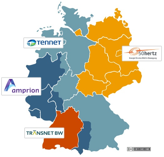
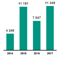
Figure 1: (Left) Control areas of German tsos. Source: Bundeszentrale für politische Bildung, 2013, www.bpb.de. (Right) Annual re-dispatch (in GWh) of German tsos. Data source: netztransparenz.de

Within the usual time interval of 15 min a power plant can change its setpoint only incrementally. Thus, in real-world applications (multi-stage quasi-stationary) opf problems are subject to hidden constraints that can be expressed as discrete-time dynamics. Put differently, opf leads naturally to large-scale non-convex discrete-time optimal control problems. Moreover, as the Energiewende induces uncertainties (volatile renewables, uncertain future market solutions, …) there is a tremendous need for scalable methods tackling opf problems. Hence, in the present paper we aim at providing a unified framework to multi-stage predictive, distributed and stochastic opf. Moreover, the paper is meant as an introduction tailored to readers with background in systems and control who are not yet familiar with opf. This scope implies that we do neither claim completeness in terms of literature overview, nor do we discuss the most general variants of opf problems.

We begin with a concise statement of the opf problem in Section 2 commenting on usual relaxations. Section 3 entails the main contribution of this paper; i.e. a control-specific formulation of research challenges all of which entail opf problems and variants thereof at their core. This includes blueprint formulations for multi-stage quasi-stationary predictive opf, distributed (multi-agent) formulations, opf with stochastic uncertainties, and comments on further opf variants. Moreover, in Section 4 we sketch control-specific open problems. Finally, the paper closes with conclusions in Section 5.

2 Optimal Power Flow – Problem Statement

There exists a plethora of references on opf, see [102, 26, 40, 22, 19]. Subsequently, we present a concise formulation of opf problems that enables the statement of control-specific research challenges in Section 3.

2.1 The Power Flow Equations

We consider balanced electrical ac grids as lumped-parameter systems at steady state, which can be modeled by the triple $(\mathcal{N},\mathcal{G},Y)$, where $\mathcal{N}=\{1,\ldots,N\}$ is the set of buses (nodes), $\mathcal{G}\subseteq\mathcal{N}$ is the non-empty set of generators, and $Y=G+\mathrm{j}B\in\mathbb{C}^{N\times N}$ is the bus admittance matrix [43]. Moreover, we assume symmetric three-phase ac conditions. Every bus $l\in\mathcal{N}$ is described by its voltage phasor $v_{l}\mathrm{e}^{j\theta_{l}}\in\mathbb{C}$ and net apparent power $s_{l}=p_{l}+jq_{l}\in\mathbb{C}$, or equivalently by its voltage magnitude $v_{l}$, voltage phase $\theta_{l}$, net active power $p_{l}$, and net reactive power $q_{l}$.

2.1.1 AC Power Flow

The power flow equations describe the steady-state behavior of an ac electrical network in terms of the voltage phasors and net apparent powers

$$p_{l}= \;v_{l}\sum_{m\in\mathcal{N}}v_{m}(G_{lm}\cos(\theta_{lm})+B_{lm}\sin(\theta_{lm})),$$ (1a)

$$q_{l}= \;v_{l}\sum_{m\in\mathcal{N}}v_{m}(G_{lm}\sin(\theta_{lm})-B_{lm}\cos(\theta_{lm})),$$ (1b)

where $\theta_{lm}:=\theta_{l}-\theta_{m}$. Observe that in the power flow equations (1) the phase angles $\theta_{l}$ occur as pair-wise differences, therefore one bus $l_{0}\in\mathcal{N}$ is specified as reference (slack) bus $\theta_{l_{0}}=0$ for $l_{0}\in\mathcal{N}$; w.l.o.g. we consider $l_{0}=1$ in the remainder. For the sake of simplicity, we assume that there is only one generator per bus (i.e. $\mathcal{G}\subseteq\mathcal{N}$). We describe the net apparent power of bus $l\in\mathcal{N}$ by

$$s_{l}=p_{l}+\mathrm{j}q_{l}=\begin{cases}(p_{l}^{\text{g}}-p_{l}^{\text{d}})+\mathrm{j}(q_{l}^{\text{g}}-q_{l}^{\text{d}}),&l\in\mathcal{G},\\ -p_{l}^{\text{d}}-\mathrm{j}q_{l}^{\text{d}},&\text{otherwise},\end{cases}$$

where $p_{l}^{\text{g}}$, $q_{l}^{\text{g}}$ are controllable power injections for all generator nodes $l\in\mathcal{G}$, and $p_{l}^{\text{d}}$, $q_{l}^{\text{d}}$ are uncontrollable power sinks/sources for all $l\in\mathcal{N}$, cf. Figure 2.

Figure 2: Power generation, demand and net power at node $l$.

Hence, we define the control input $u\in\mathbb{R}^{n_{u}}$, the disturbance $d\in\mathbb{R}^{n_{d}}$, and the state $x\in\mathbb{R}^{n_{x}}$ as follows

$$u =\begin{pmatrix}p_{l}^{\text{g}}&q_{l}^{\text{g}}\end{pmatrix}_{l\in\mathcal{G}}^{\top}\in\mathbb{R}^{n_{u}}, n_{u}=2|\mathcal{G}|,$$ (2a)

$$d =\begin{pmatrix}p_{l}^{\text{d}}&q_{l}^{\text{d}}\end{pmatrix}^{\top}_{l\in\mathcal{N}}\in\mathbb{R}^{n_{d}}, n_{d}=2|\mathcal{N}|,$$ (2b)

$$x =\begin{pmatrix}v_{l}&\theta_{l}\end{pmatrix}_{l\in\mathcal{N}}^{\top}\in\mathbb{R}^{n_{x}}, n_{x}=2|\mathcal{N}|.$$ (2c)

We remark that depending on the specific problem at hand, one may also consider the voltage of a bus as an additional input variable. Our choice of state and input variables allows writing the power flow equations (1) in terms of a system of nonlinear algebraic equations

$$F:\mathbb{R}^{n_{x}}\times\mathbb{R}^{n_{u}}\times\mathbb{R}^{n_{d}}\rightarrow\mathbb{R}^{2N}\qquad F(x,u;d)=0,$$ (3)

where the semicolon notation emphasizes the dependency on the exogenous disturbance $d$. For the sake of concise notation, we introduce the so-called power-flow manifold

$$\mathcal{F}(d):=\left\{(x~{}u)^{\top}\in\mathbb{R}^{n_{x}+n_{u}}\,|\,F(x,u;d)=0\right\}$$ (4)

describing all solutions to the power-flow equations (1) for a given disturbance $d$. Since (1) states $2N$ equality constraints and we consider $4N$ variables, the differentiable manifold $\mathcal{F}(d)$ is of dimension $2N$. As we will see later, it determines the number of degrees of freedom remaining for optimization.

Note that in this section we have formulated the power-flow equations in polar coordinates. However, resorting to Cartesian coordinates—i.e. swapping voltage magnitude $v_{l}$ and phase $\theta_{l}$ with the imaginary and real part of the voltage—they can equivalently be written as a set of polynomial equations [40].

2.1.2 DC Power Flow

To the end of obtaining a linear approximation of the power flow equations (1), one typically assumes the following: lossless lines ($r_{lm}\approx 0$ for the Ohmic resistance of the line connecting buses $l$ and $m$), small phase differences ($\theta_{lm}=\theta_{l}-\theta_{m}\approx 0$), constant voltage magnitudes ($v_{l}\approx 1$). Under these assumptions—which typically hold for high-voltage transmission systems—the ac active power flow equations (1) simplify to

$$p_{l}= \;-\sum_{m\in\mathcal{N}\setminus\{l\}}b_{lm}(\theta_{l}-\theta_{m})\quad\Longleftrightarrow\quad p=-B\theta,$$ (5)

where $B$ is the imaginary part of the bus admittance matrix $Y$. The above equations (5) are the so-called dc power flow equations [43]. Note that in the absence of shunts elements the reactive power flows vanish due to the assumptions of small angle differences and constant voltages. Compared to ac power flow, the control input $u^{\text{{dc}}}\in\mathbb{R}^{n_{u^{\text{{dc}}}}}$, the disturbance $d^{\text{{dc}}}\in\mathbb{R}^{n_{d^{\text{{dc}}}}}$, and the state $x^{\text{{dc}}}\in\mathbb{R}^{n_{x^{\text{{dc}}}}}$ for dc power flow become

$$u^{\text{{dc}}} =\begin{pmatrix}p_{l}^{\text{g}}\end{pmatrix}_{l\in\mathcal{G}}^{\top}\in\mathbb{R}^{n_{u^{\text{{dc}}}}}, n_{u^{\text{{dc}}}}=|\mathcal{G}|,$$

$$d^{\text{{dc}}} =\begin{pmatrix}p_{l}^{\text{d}}\end{pmatrix}^{\top}_{l\in\mathcal{N}}\in\mathbb{R}^{n_{d^{\text{{dc}}}}}, n_{d^{\text{{dc}}}}=|\mathcal{N}|,$$

$$x^{\text{{dc}}} =\begin{pmatrix}\theta_{l}\end{pmatrix}_{l\in\mathcal{N}}^{\top}\in\mathbb{R}^{n_{x^{\text{{dc}}}}}, n_{x^{\text{{dc}}}}=|\mathcal{N}|.$$

From this it follows that the net power $p$ is $p=u^{\text{{dc}}}+d^{\text{{dc}}}$. In terms of the compact notation (3) and (4) we obtain

$$F^{\text{{dc}}}(x^{\text{{dc}}},u^{\text{{dc}}};d^{\text{{dc}}})=u^{\text{{dc}}}-d^{\text{{dc}}}+Bx^{\text{{dc}}}=0,$$

and

$$\mathcal{F}^{\text{{dc}}}(d^{\text{{dc}}}):=\left\{(x^{\text{{dc}}}~{}u^{\text{{dc}}})^{\top}\in\mathbb{R}^{n_{x^{\text{{dc}}}}+n_{u^{\text{{dc}}}}}\,|\,F^{\text{{dc}}}(x^{\text{{dc}}},u^{\text{{dc}}};d^{\text{{dc}}})=0\right\}.$$ (7)

2.2 Optimal Power Flow

Besides the power flow equations (1) engineering requirements are usually considered in terms of box constraints as follows

$$u\in\mathcal{U} =\left\{\begin{pmatrix}p_{l}^{\text{g}}&q_{l}^{\text{g}}\end{pmatrix}_{l\in\mathcal{G}}^{\top}\in\mathbb{R}^{n_{u}}:\quad p_{l}^{\text{g}}\in[\underline{p}_{l}^{\text{g}}\,,\overline{p}_{l}^{\text{g}}],\quad q_{l}^{\text{g}}\in[\underline{q}_{l}^{\text{g}},\,\overline{q}_{l}^{\text{g}}]\right\}$$ (8a)

$$x\in\mathcal{X} =\left\{\begin{pmatrix}v_{l}&\theta_{l}\end{pmatrix}_{l\in\mathcal{N}}^{\top}\in\mathbb{R}^{n_{x}}:\quad v_{l}\in[\underline{v}_{l},\,\overline{v}_{l}],\>\forall l\in\mathcal{N},\quad\theta_{l_{0}}=0\right\}.$$ (8b)

Actually, the constraints (8) are a simplification of the true technical requirements. For example, generator curves may impose constraints that couple $p_{l}^{\text{g}}$, $q_{l}^{\text{g}}$, and $v_{l}$ at generator bus $l\in\mathcal{G}$; binary constraints may be imposed when shunts and/or generators can be turned on and off.

Additional constraints comprise limits on the line flows, which are often modeled as constraints on the magnitude of apparent power

$$|s_{lm}|=\sqrt{p_{lm}^{2}+q_{lm}^{2}}\leq|\bar{s}_{lm}|,\quad\forall(l,m)\in\mathcal{L},$$ (9a)

where $$\mathcal{L}\subseteq\mathcal{N}\times\mathcal{N} M=|\mathcal{L}| p_{lm} l m p_{lm} q_{lm}$$ is the set of lines, with being the number of lines. The active power across the line connecting buses to , , and the corresponding reactive power are given by

$$p_{lm} =\hphantom{-}v_{l}^{2}g_{lm}-v_{l}v_{m}(g_{lm}\cos(\theta_{lm})+b_{lm}\sin(\theta_{lm})),$$ (9b)

$$q_{lm} =-v_{l}^{2}b_{lm}+v_{l}v_{m}(b_{lm}\cos(\theta_{lm})-g_{lm}\sin(\theta_{lm})),$$ (9c)

where $b_{lm}$ and $g_{lm}$ are line parameters. The line flows (9) depend only on the state $x$, and can be written compactly as

$$c:\mathbb{R}^{n_{x}}\rightarrow\mathbb{R}^{|\mathcal{L}|}\qquad\qquad s_{\text{line}}=c(x).$$ (10)

This allows for the compact notation

$$\mathcal{C}:=\left\{x\in\mathbb{R}^{n_{x}}\,|\,c(x)\leq\begin{pmatrix}|\bar{s}_{lm}|\end{pmatrix}_{(l,m)\in\mathcal{L}}^{\top}\right\}\subset\mathbb{R}^{n_{x}},$$ (11)

where the inequality is evaluated component-wise.

2.2.1 AC OPF

Typical objectives considered in opf span from the minimization of active power generation costs via the minimization of transmission losses to suppressing overly large injections of reactive power, see e.g. [40]. Frequently, the cost function $J:\mathbb{R}^{n_{u}}\rightarrow\mathbb{R}$ is assumed to be convex (often quadratic) in the argument $u$. Summarizing all of the above, the single-stage ac opf problem is given by

$$\min_{(x,u)\in\mathbb{R}^{n_{x}+n_{u}}}\quad J(u)$$ (12a)

subject to

$$(x,~{}u)^{\top} \in\mathcal{F}(d),$$ (12b)

$$u \in\mathcal{U},$$ (12c)

$$x \in\mathcal{X},$$ (12d)

$$x \in\mathcal{C}.$$ (12e)

The main challenges in solving the ac opf as given above are: the non-convexity of the sets $\mathcal{F}(d)$ and $\mathcal{C}$, the fact that the objective is not strictly convex in $x$ and $u$, and the fact that realistic grid models can easily comprise several thousand nodes [91, 95].

Note that there exist powerful software packages to solving (12) such as Matpower [103] (which is an open-source Matlab toolbox specific for opf), jump [30] (which is an open-source Julia nlp package) or CasADi [2] (which is an open-source nlp package available for Matlab and Python). In general, one can distinguish the following main approaches to solving (12):

• tackling it as a generic nlp [22, 72, 102, 40];

• alternating solution of the power-flow equations (1) and minimizing a quadratic objective [50, 89];

• polynomial reformulation and semi-definite relaxation of the power-flow equations (1) [7, 65, 66, 68]; and

• affine approximation of the sets $\mathcal{F}(d)$ and $\mathcal{C}$ which is discussed next.

2.2.2 DC OPF

For dc power flow conditions, the box constraints for the input $u^{\text{{dc}}}$ and the state $x^{\text{{dc}}}$ are obtained from (8) by removing the entries referring to the reactive power and the voltage magnitude respectively

$$u^{\text{{dc}}}\in\mathcal{U}^{\text{{dc}}} :=\left\{\begin{pmatrix}p_{l}^{\text{g}}\end{pmatrix}_{l\in\mathcal{G}}^{\top}\in\mathbb{R}^{n_{u}}:\quad p_{l}^{\text{g}}\in[\underline{p}_{l}^{\text{g}},\overline{p}_{l}^{\text{g}}]\quad\forall l\in\mathcal{G}\right\}$$

$$x^{\text{{dc}}}\in\mathcal{X}^{\text{{dc}}} :=\left\{\begin{pmatrix}\theta_{l}\end{pmatrix}_{l\in\mathcal{N}}^{\top}\in\mathbb{R}^{n_{x}}:\quad\theta_{l_{0}}=0\right\}.$$

Under dc conditions the function $c^{\text{{dc}}}:\mathbb{R}^{n_{x^{\text{{dc}}}}}\rightarrow\mathbb{R}^{|\mathcal{L}|}$ in (10)—that maps the state to the line flows—is obtained from Kirchhoff’s laws as $c^{\text{{dc}}}(x^{\text{{dc}}})=-B_{\text{br}}Ax^{\text{{dc}}}$, where $B_{\text{br}}=\operatorname{diag}((b_{lm})_{(l,m)\in\mathcal{L}}^{\top})\in\mathbb{R}^{M\times M}$ is the branch susceptance matrix, and $A\in\mathbb{R}^{M\times N}$ is the graph incidence matrix. This leads to

$$\mathcal{C}^{\text{{dc}}}:=\left\{x^{\text{{dc}}}\in\mathbb{R}^{n_{x^{\text{{dc}}}}}|-B_{\text{br}}Ax^{\text{{dc}}}\leq\begin{pmatrix}\bar{p}_{lm}\end{pmatrix}_{(l,m)\in\mathcal{L}}^{\top}\right\}\subset\mathbb{R}^{n_{x^{\text{{dc}}}}}.$$

Summing up, the single-stage dc opf problem can be posed as follows

$$\min_{(x^{\text{{dc}}},\,u^{\text{{dc}}})\in\mathbb{R}^{n_{x^{\text{{dc}}}}+n_{u^{\text{{dc}}}}}}\quad J(u^{\text{{dc}}})$$ (14a)

subject to

$$(x^{\text{{dc}}},~{}u^{\text{{dc}}})^{\top} \in\mathcal{F}^{\text{{dc}}}(d^{\text{{dc}}}),$$ (14b)

$$u^{\text{{dc}}} \in\mathcal{U}^{\text{{dc}}},$$ (14c)

$$x^{\text{{dc}}} \in\mathcal{X}^{\text{{dc}}},$$ (14d)

$$x^{\text{{dc}}} \in\mathcal{C}^{\text{{dc}}}.$$ (14e)

Observe that, for usual choices of $J$, (14) is a quadratic program positive definite in $u^{\text{{dc}}}$. Hence dc opf is structurally considerably simpler than ac opf. Finally, note that it is straightforward to eliminate the state $x^{\text{{dc}}}$ from (14). This yields smaller optimization problems that are strictly convex in the decision variable $u^{\text{{dc}}}$.

3 Advanced OPF Variants

After the introduction of the opf problem in its simple single-stage ac and dc variants, it deserves to be noted that in the power systems community these problems are for the most part well understood, see [43, 72, 102, 40]. At the same time Problem (12) and Problem (14) as such are rarely solved in practice. Indeed, quite often one has to tackle more advanced variants thereof. The purpose of this section is to provide a tutorial introduction to selected advanced problems that are of relevance in different operational contexts (unit commitment, …). Moreover, we outline how the systems-and-control approaches could contribute to tackling them.

3.1 Multi-Stage and Predictive OPF

From a systems and control perspective, Problem (12) and Problem (14) are steady-state optimization problems. Due to the well-known time scale separation underlying the conventional control paradigm of primary, secondary and tertiary control (cf. Fig. 3), opf problems are often solved on the basis of 15 min sampling intervals. While the fast transients of power systems are clearly settling much faster (in the order of milliseconds up to a few minutes), a large-scale power plant cannot change its setpoint arbitrarily on a 15 min interval. Rather it is subject to ramp constraints that give raise to (quasi-stationary) multi-stage opf problems.

To the end of concise notation, henceforth the argument $\cdot(k)$ denotes the time index $k\in\mathbb{N}$ of a variable. We consider ramp constraints for the generators, i.e. constraints of the form

Figure 3: Time scales in power systems according to [1].

$$p_{l}(k+1)-p_{l}(k)\in[\Delta\underline{p}_{l},\Delta\overline{p}_{l}],l\in\mathcal{G}.$$

Using the shorthand notation (2a), it is straightforward to see that these constraints can be expressed in form of the following discrete-time system

$$u(k+1)=u(k)+\delta u(k),\qquad u(0)=u_{0}.$$

Here $\delta u(k)\in\mathbb{R}^{n_{u}}$ is the incremental change of active generator powers constrained by

$$\delta\mathcal{U}:=\underset{l\in\mathcal{G}}{\bigtimes}\,\,\left([\Delta\underline{p}_{l},\Delta\overline{p}_{l}]\times\mathbb{R}\right)\,\subset\mathbb{R}^{n_{u}}.$$

Note that the ramp constraints are typically only imposed on active power and not on reactive power.

3.1.1 Multi-Stage AC OPF

The multi-stage AC opf problem can now be stated as

$$\min_{(x(\cdot),u(\cdot),\delta u(\cdot))\in\mathbb{R}^{(n_{x}+2n_{u})T}}\quad \sum_{k\in\mathcal{T}}J(u(k))+\|\delta u(k)\|_{\Sigma}^{2}$$ (15a)

subject to $$\forall k\in\mathcal{T}$$

$$u(k+1) =u(k)+\delta u(k),\qquad u(0)=u_{0},$$ (15b)

$$\delta u(k) \in\delta\mathcal{U},$$ (15c)

$$(x(k),\,u(k))^{\top} \in(\mathcal{X}\times\mathcal{U})\cap\mathcal{F}(d(k)),$$ (15d)

$$x(k) \in\mathcal{C},$$ (15e)

where $\mathcal{T}=\{0,1,\dots,k,\dots,T-1\}\subset\mathbb{N}$ denotes the set of considered time instants.

Observe that, for the sake of generality, we introduce the quadratic penalty $\|\delta u(k)\|_{\Sigma}^{2}$ with $\Sigma\succeq 0$ to regularize the optimization with respect to the incremental input change $\delta u(k)$. Moreover, Problem (15) looks structurally similar to discrete-time optimal control problems arising in the context of Nonlinear Model Predictive Control (nmpc) [84, 44]. From an nmpc point of view, $\delta u(k)$ takes the role of the input, $u(k)$ is the dynamic state, $x(k)$ can be regarded as some kind of algebraic state variable, and $d(k)$ is an exogenous disturbance signal. Note that inclusion of energy storages (batteries, pumped-hydro, etc.) will lead to additional dynamics. Due to space limitations, we do not discuss this in detail here. Moreover, it is easy to see that Problem (15) is non-convex. However, considering the DC formulation from Section 2.2 convex approximation is straightforward, see e.g. [49, 48].

Example – IEEE 5 Bus

Next, we consider a simple example of a multi-stage opf problem. Fig. 4 depicts the modified ieee 5 bus case [64] with time-varying load at node 4 and a generator ramp constraint at the cheapest generator at node 1. The objective $J$ is given by a quadratic function $J(u)=u^{\top}Hu+h^{\top}u,\quad H\succeq 0$, with $H=\mathrm{diag}(200,0,220,240,260,\boldsymbol{0})$, $h=(1500,0,3000,4000,1000,\boldsymbol{0})^{\top}$, where $\boldsymbol{0}$ is a vector (of appropriate dimensions) corresponding to zero cost on reactive power injection. Note that we do not consider regularization with respect to $\delta u(k)$.

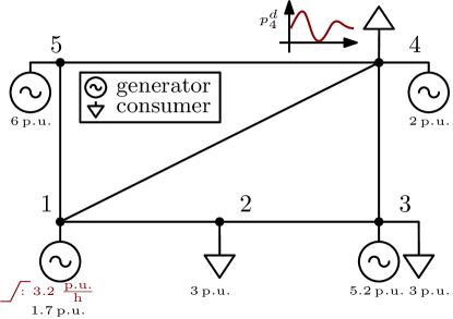
Figure 4: ieee 5 bus system with time-varying load at node 4 and generator ramp constraint at node 1.

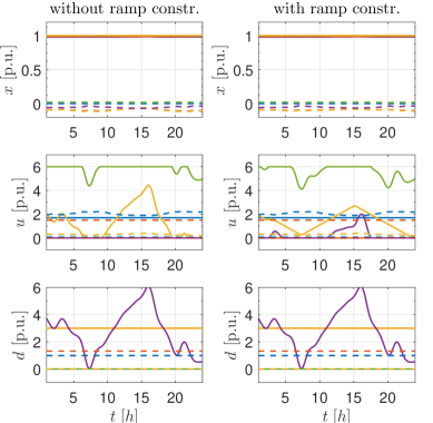
Figure 5: Results for the ieee 5 bus case without (left) and with (right) ramp constraints.

Fig. 5 shows numerical results in case with and without active ramp constraint at node 1. We formulate the problem as an nlp and solve it via CasADi and ipopt in Matlab [2]. Therein, the first row depicts the states consisting of phase angles $\theta$ (dashed) and voltage magnitudes $v$ (solid), the second row depicts the controls consisting of active and reactive power injections $p$ (solid) and $q$ (dashed), and the last row shows the (time varying) parameter vector $p$ consisting of active and reactive power demands $p^{d}$ (solid) and $q^{d}$ (dashed). One can observe that the time-varying demand of node 4 is mainly covered by the generators at node 1 and 5 since they are the cheapest and, hence, generator 5 is almost always on its upper limit. Introducing a ramp constraint of 3.2 p.u./h for generator 1, the limited ramping capability has to be compensated by generator 3 (purple line) which has not been used in the former case. In turn this leads to higher total cost of 42 930 US$ compared to 42 166 US$ for the case without ramp constraints.

3.2 Distributed OPF

Given the size of opf problems (up to several thousands of nodes) and considering their importance it is not surprising that there exists a large body of literature on distributed approaches to opf, see e.g. [35, 70, 54, 80, 25]. However, computational feasibility is not the sole motivation for distributed solutions to opf problems. Indeed, distributed algorithms promise grid operation with a reduced need for centralized coordination. In other words, there is hope that in case of blackouts or other emergencies distributed entities will show more resilience than centralized approaches [59, 25].

Moreover, the current structure of the power system is inherently interconnected. For example, Germany’s high-voltage transmission grid is operated by four different tsos, cf. Figure 1. On a lower level, about 890 Distribution System Operators (dsos) operate the underlying distribution grids. Thus, the steadily increasing need for coordination of the different players calls for tailored numerical methods. At the same time it may be desirable to avoid accumulation of data at a single entity.

In distributed optimization one typically discusses problems with separable objectives and partially separable constraints, whereby the sole coupling is given by affine equalities [11, 9]; i.e. problems of the following form:

$$\min_{(x,\,u)\in\mathbb{R}^{n_{u}+n_{x}}}\quad \sum_{i\in\mathcal{R}}J_{i}(u_{i})$$ (16a)

subject to

$$h_{i}(x_{i},u_{i}) \leq 0,\qquad\quad i\in\mathcal{R},$$ (16b)

$$\sum_{i\in\mathcal{R}}A_{i}\cdot(x_{i} ,u_{i})^{\top}=b.$$ (16c)

The underlying idea is that state and control vectors $x$ and $u$ are partitioned into $\mathcal{R}=\{1,\dots,R\}$ local state and control vectors $x_{i}\in\mathbb{R}^{n_{x{}i}}$ and $u_{i}\in\mathbb{R}^{n_{u{}i}}$ that correspond to the subproblems. These subproblems involve possibly non-convex constraints $h_{i}:\mathbb{R}^{n_{x{}i}}\times\mathbb{R}^{n_{u{}i}}\rightarrow\mathbb{R}^{n_{hi}}$. The objective function should be a sum of local terms depending on distinct partitions of the controls only; constraint coupling should take place via an affine so-called consensus constraint (16c). Apparently, one needs to slightly reformulate Problem (12) to be consistent with Problem (16).

3.2.1 Separable Reformulation of AC OPF

In order to fit into the form of (16), one can reformulate Problem (12) by partitioning the set of buses $\mathcal{N}$ into $\mathcal{R}=\{1,\dots,R\}$ disjoint subsets $\mathcal{N}_{i}=\{n_{i}^{1},\dots,n_{i}^{N_{i}}\}\subset\mathcal{N}$ such that $\bigcup_{i\in\mathcal{R}}\mathcal{N}_{i}=\mathcal{N}$ and $\mathcal{N}_{i}\cap\mathcal{N}_{j}=\emptyset$ for all $i\neq j$. Then, one introduces two additional so-called auxiliary nodes in the middle of each line that connects two neighboring partitions. Thus, the node set $\mathcal{N}$ is enlarged to $\mathcal{N}^{A}=\{1,\dots,N,\dots,N+A\}$ which also contains these auxiliary nodes. Consider an auxiliary node pair with indexes $k$ and $l$. In order to maintain equivalence to the original opf problem, all values at these auxiliary node pairs should match

$$\theta_{k} =\theta_{l}, p_{k} =-p_{l},$$

$$v_{k} =v_{l}, q_{k} =-q_{l}.$$

Rewriting these equality constraints in matrix form yields $A_{i}$ and $b$ for the consensus constraint in (16c). Quite often, the objective of Problem (12) is the sum of squared generator powers. Hence, the objective function of (16) can be obtained by selecting (and possibly rearranging) the corresponding blocks to the input partitions $u_{i}$, cf. [32] for a tutorial example.

Partitioning of $\mathcal{N}^{A}$ enables splitting the (nonlinear and non–convex) constraints (4)–(11) into local inequality constraints $h_{i}$. To this end, the power flow equations (1) are formulated for all partitions $\mathcal{N}_{i}$ individually obtaining $\mathcal{F}_{i}(d_{i})$ for all $i\in\mathcal{R}$. The same can be done for the line limits (9) and state/input constraint sets $\mathcal{X}$, $\mathcal{U}$ obtaining $\mathcal{C}_{i}(d)$, $\mathcal{X}_{i}$, and $\mathcal{U}_{i}$ respectively.

Henceforth, for the sake of compact notation, we collect all constraints forming the constraint sets on local state constraints $\mathcal{X}_{i}$, input constraints $\mathcal{U}_{i}$ and the nonlinear power flow/line flow constraints $\mathcal{F}_{i}(d_{i})$ in one vector-valued local inequality constraint per partition

$$h_{i}(x_{i},u_{i})\leq 0,\qquad i\in\mathcal{R}$$

with $h_{i}:\mathbb{R}^{n_{x{}i}}\times\mathbb{R}^{n_{u{}i}}\rightarrow\mathbb{R}^{n_{hi}}$ completing the opf problem in affine-coupled separable form (16).

3.2.2 Brief Overview of Existing Approaches

There are several research challenges for the design of distributed opf algorithms [57]. First of all, the algorithms should be able to solve non-convex ac opf problems reliably even when initialized far from a local minimum; additionally they should converge sufficiently fast and exchange as little information as possible and, finally they should comprise a low-complexity coordination step (ideally based on neighbor-to-neighbor communication). Furthermore, it is desirable to allow considering problem partitions related to “operational practice”; i.e. to be able to mirror the actual tsos regulation zones.

Many classical distributed optimization algorithms tailored to convex problems are—despite a lack of convergence guarantees—often applied to non-convex ac opf problems directly. Early works employ the Auxiliary Problem Principle [59, 56], the Predictor Corrector Proximal Multiplier Method [58] and more recently the very popular Alternating Direction of Multipliers Method (admm) [58, 34]. Especially admm has gained significant attention; thereby performing exhaustive simulation-based convergence analysis [34], investigating parameter update rules [35], and finally analyzing applicability to large-scale systems [46]. However, for all the aforementioned algorithms convergence can, in general, not be guaranteed due to non-convexity. Moreover, the observed convergence is often slow; especially when tight solution tolerances are needed [11, 9].

Alternatively, a method denoted as Optimality Condition Decomposition is proposed in [24, 23] and is extended in [80, 5, 55]. This method performs well in many practical cases, however, there is an ongoing discussion on whether the convergence result of [24] holds for generic ac opf problems [34].

There are two major research lines dealing with the issue of convergence guarantees:

• convexifying ac opf by either the dc opf or by an (inner or outer) convex approximation of the feasible set and then applying one of the convex optimization algorithms mentioned before;

• designing new algorithms capable of handling non-convex ac opf problems directly.

With respect to (i) recall that the ac opf problem can be written as a problem with quadratic equality constraints, see e.g. [40]. Thus it can be cast as a rank-constrained Semi-Definite Program (sdp) in a higher dimensional space. Dropping the non-convex rank constraint yields a convex sdp that can be solved with convergence guarantees [7, 25, 71, 82]. One limitation of the sdp approach is that the solution obtained from the convex relaxation might not satisfy the rank constraint and hence, the solution of the original problem can not be recovered. However, there exist technical conditions (usually structural assumptions on grid components like transformers or on the grid topology) under which the exactness can be guaranteed [63, 65, 66].

Research line (ii) investigates recently developed distributed optimization algorithms capable of solving non-convex problems directly with convergence guarantees. One can distinguish two main approaches: Either one distributes distinct steps of centralized algorithms like interior point or sequential quadratic programming inheriting all their mathematical properties, or one develops entirely new algorithms which directly exploit the structure of separable optimization problems. For the former, there exists approaches for distributing steps of centralized interior point methods [67], or, in the context of optimal control, there exist methods distributing steps of sequential quadratic programming [78, 94]. For the latter, [52] presents an approach based on alternating projections combined with a trust-region globalization. Recently, a subset of the authors of the present paper proposed to use the Augmented Lagrangian Alternating Direction Inexact Newton Method (aladin) providing convergence guarantees and fast convergence behavior [31, 32]. Table 1 provides a summary overview of existing distributed approaches to opf.

Table 1: Overview of distributed optimization methods applied to ac opf.

	ADMM	ADMM-SDP	Alternating Trust Region	ALADIN
Convergence guarantee	no	(yes)	yes	yes
Observed convergence rate	(linear)	linear	linear	quadratic
Communication effort	low	low/medium	low/medium	medium/high
Selected references	[34, 46]	[25]	[52]	[31, 32]

3.2.3 Example – IEEE 14 Bus via ALADIN

As an example for solving ac opf (12) in a hierarchical distributed fashion, we apply the aladin algorithm to the ieee 14 bus test system. We start by briefly recalling aladin, for a more detailed description of aladin we refer to [53].

In step 1) of Algorithm 1, the local nlps (17) are solved obtaining local optimal inputs and state vectors $z_{i}=(x_{i},u_{i})$ for all $i\in\mathcal{R}$. In these nlps an augmented Lagrangian function is minimized with respect to the consensus constraint of Problem (16). The Lagrange multipliers $\lambda^{k}$ and $\bar{z}_{i}^{k}$ are treated as fixed parameters. Step 2) computes local derivatives; i.e. gradients $g_{i}^{k}$, Hessians $H_{i}^{k}$ and Jacobians $C_{i}^{k}$ of the active constraints. The index set of active constraints (inequality constraint holding with equality) at $(z_{i}^{k})$ is defined by $\mathcal{A}_{i}(z_{i}^{k})=\{\;j\;\,|\;\,(h_{i})_{j}(z_{i}^{k})=0\;\}$ and communicated to the coordinating entity. Observe that in many cases these derivatives do not have to be computed explicitly as they are returned by the solvers applied to (17). In the following step 3), all derivatives from the local problems are collected, aggregated in global derivatives $g^{k}$, $H^{k}$ and $C^{k}$, and an equality constrained coordination qp is solved. This is computationally cheap as solving this qp leads to a linear system of equations where very efficient solvers exist. Finally, step 4) updates the solution guesses and performs a line search if necessary (this step can be omitted in many cases, cf. [32]). The very last step applies a problem-specific heuristic to update $\rho$ and $\mu$.

Result: $z^{\star}$

Input:$\quad\bar{z}^{0},\;\lambda^{0},\;\rho,\;\Sigma_{i},\;\mu,\;$ $k=0$

while $\left\|Az^{k}\right\|_{\infty}>\epsilon$ and $\rho\,\left\|z^{k}-\bar{z}^{k}\right\|_{\infty}>\epsilon$  do

      

      1) Solve local problems

$$z_{i}^{k}=\underset{z_{i}}{\text{arg}\min} \quad f_{i}(z_{i})+(\lambda^{k})^{\top}A_{i}z_{i}+\frac{\rho^{k}}{2}\left\|z_{i}-\bar{z}_{i}^{k}\right\|_{\Sigma_{i}}^{2}\quad$$

s.t. $$\quad h_{i}(z_{i})\leq 0\quad\mid\kappa_{i}^{k}.$$ (17)

      2) Compute gradients & Hessians for QP

      Obtain gradients $g_{i}^{k}$, Hessian of the Lagrangians $B_{i}^{k}$ the Jacobian of the active constraints $C_{i}^{k}$

      3) Solve coordination QP Solve the coordination qp

$$\underset{\Delta z_{i},s}{\min}\;\;\sum_{i\in\mathcal{R}}\left\{\frac{1}{2}\Delta z_{i}^{\top}B^{k}_{i}\Delta z_{i}+{g_{i}^{k}}^{\top}\Delta z_{i}\right\}+(\lambda^{k})^{\top}s+\frac{\mu^{k}}{2}\|s\|^{2}_{2}$$

$$\begin{aligned} \qquad\qquad\text{s.t.}\;\qquad\qquad\quad C^{k}\Delta z_{i}&=0\\ \quad\sum_{i\in\mathcal{R}}A_{i}(z_{i}^{k}+\Delta z_{i})&=s\quad|\;\lambda^{\mathrm{QP}},\end{aligned}$$ (18)

obtaining $\Delta z^{k}$ and $\lambda^{\text{QP}}$.

      4) Line search Update primal and dual variables by

$$\bar{z}_{i}^{k+1} \leftarrow z_{i}^{k}+\alpha^{k}_{1}\left(z_{i}^{k}-\bar{z}_{i}^{k}\right)+\alpha_{2}^{k}\Delta z_{i}^{k}\;,$$

$$\lambda^{k+1} \leftarrow \lambda^{k}+\alpha^{k}_{3}(\lambda^{\mathrm{QP}}-\lambda^{k}),$$

with $\alpha^{k}_{1},\alpha^{k}_{2},\alpha^{k}_{3}$ from [53]. If full step is accepted, i.e. $\alpha_{1}^{k}=\alpha_{2}^{k}=\alpha_{3}^{k}=1,$ update $\rho^{k}$ and $\mu^{k}$ by

$$\rho^{k+1}\;(\mu^{k+1})=\begin{cases}r_{\rho}\rho^{k}\;(r_{\mu}\mu^{k})&\text{if}\;\rho^{k}<\bar{\rho}\;\;(\mu^{k}<\bar{\mu})\\ \rho^{k}\;(\mu^{k})&\text{otherwise}\end{cases}.$$

end while

Algorithm 1 aladin algorithm.

Conceptually, aladin can be regarded as a combination of admm and an sqp method; i.e. the local steps are very similar to the ones of admm, but the coordination step is similar to sqp. Furthermore, it is possible to express admm as a special case of aladin by appropriate choice of parameters [53].

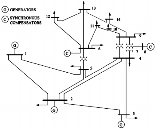
Figure 6: IEEE 14 bus test system with $\mathcal{N}_{1}=\{1,2,5\}$, $\mathcal{N}_{2}=\{3,4,7\text{\,-\,}9\}$, $\mathcal{N}_{3}=\{6,10\text{\,-\,}14\}$.

We consider the ieee 14 bus test system shown in Fig. 6 as an illustrative example. We divide the grid into $\mathcal{R}=\{1,2,3\}$ partitions motivated by geographical considerations. Due to space limitations, we omit commenting on the parameter tuning for aladin here. We refer to [32, 31] for an opf–specific discussion. We solve the problem via CasADi and ipopt in Matlab [2]. Fig. 7 shows the numerical results of aladin for the described test system. Specifically, we plot the distance to the “true” minimizer $\|z^{k}-z^{\star}\|_{\infty}$, the consensus violation $\|Az^{k}\|$—which indicates to which extent the physical values (active/reactive power and voltages) at the auxiliary nodes match—and the active power injections $p$ (which partially represents the controls $u$) over the iteration index $k$. For all these indicators, aladin converges to high accuracy in less than 15 iterations. Compared to admm, this is significantly faster: admm usually needs at least around hundred iterations to attain medium accuracy for problems of similar size, cf. [35, 32].

However, note that the complexity per iteration of aladin compared to admm is higher. Whereas admm exchanges local solution guesses $z_{i}^{k}$ only, aladin additionally communicates derivatives of the objective and the constraints which increases the per step communication need. Furthermore, the coordination step is more complicated because aladin requires the solution of a linear system of equations whereas for admm this system can be reduced to the computation of averages [11].

Figure 7: Numerical results for the ieee 14 bus test system.

3.3 OPF with Uncertainties

Traditionally, the opf problems (12) and (14) are solved for a fixed value of the disturbance $d\in\mathbb{R}^{n_{d}}$. However, demand forecasting and the feed-in of renewable energy sources—to name just a few drivers—call for a structured consideration of uncertainties. In the presence of uncertainties it may be more adequate to model uncertain feed-in and/or uncertain demand by random variables. Importantly, opf-specific uncertainties can be modeled by Gaussian and non-Gaussian random variables [6, 21, 92].

3.3.1 Conceptual Considerations

To the end of formalizing the opf with random variables, we consider the Hilbert space of random variables of finite variance. For a given set of outcomes $\Omega$, a $\sigma$-algebra $\mathcal{A}$, and a probability measure $\mathbb{P}$, let $(\Omega,\mathcal{A},\mathbb{P})$ denote the corresponding probability space. The space

$$L^{2}(\Omega,\mathbb{P};\mathbb{R})=\left\{\mathsf{x}:\Omega\rightarrow\mathbb{R}\quad|\quad\int_{\Omega}\mathsf{x}(\tau)^{2}\mathrm{d}\mathbb{P}(\tau)\right\}~{}/~{}\mathbb{P}\text{-almost everywhere}$$ (19)

is the set of all equivalence classes of random variables of finite variance [93]. The space $L^{2}(\Omega,\mathbb{P};\mathbb{R})$ according to (19) is a Hilbert space with respect to the scalar product

$$\langle\mathsf{x},\mathsf{y}\rangle=\mathrm{E}_{\mathbb{P}}\left[\mathsf{x}\mathsf{y}\right]=\int_{\Omega}\mathsf{x}(\tau)\mathsf{y}(\tau)\mathrm{d}\mathbb{P}(\tau).$$

By slight abuse of terminology we refer to the equivalence classes simply as “random variables.” For $\mathbb{R}^{n_{x}}$-valued random vectors the following notation is introduced

$$\mathsf{x}\in L^{2}(\Omega,\mathbb{P};\mathbb{R}^{n_{x}})\quad\Longleftrightarrow\quad\mathsf{x}_{i}\in L^{2}(\Omega,\mathbb{P};\mathbb{R})\quad\forall i=1,\ldots,n_{x}.$$

That is, instead of treating the disturbance $d$ as a real-valued element of $\mathbb{R}^{n_{d}}$, we view it as a random vector $\mathsf{d}\in L^{2}(\Omega,\mathbb{P};\mathbb{R}^{n_{d}})$. Note that so far no specific kind of distribution is assumed for the disturbance; the probability measure $\mathbb{P}$ could be Gaussian, but could also refer to any other kind of distribution of finite variance. Importantly, multivariate distributions can be considered in case the Hilbert space $L^{2}(\Omega,\mathbb{P};\mathbb{R})$ is viewed as a tensor product space of appropriate univariate Hilbert spaces [93]. We continue by investigating the consequences for the opf problem (12) in case of modeling the disturbance as a random variable.

First, the power flow equations (3) will almost surely be (numerically) violated for any combination of states $x\in\mathbb{R}^{n_{x}}$ and control inputs $u\in\mathbb{R}^{n_{u}}$, because

$$F:\mathbb{R}^{n_{x}}\times\mathbb{R}^{n_{u}}\times L^{2}(\Omega,\mathbb{P};\mathbb{R}^{n_{d}})\rightarrow\mathbb{R}^{2N}:\quad F(x,u;\mathsf{d})\neq 0\quad\text{a.s.}~{}.$$

From the numerical point of view, in the presence of uncertainties the power flow equations will almost surely be violated if the state $x$ and the input $u$ are fixed real-valued quantities. However, even if the numerical solution $(x,\,u)\in\mathbb{R}^{n_{x}+n_{u}}$ violates the power flow equations, the real physical system—obeying the laws of physics—of course attains a state on the power-flow manifold corresponding to the specific input $u\in\mathbb{R}^{n_{u}}$. Any numerical deviations of the power flow equations have to be accounted for by lower-level controllers. In the view of hierarchical control of power systems it is thus desirable to obtain higher-level control inputs $u$ from opf such that the numerical solution is as close to the physical solution as possible; this ensures fewer control actions (of lower magnitude) to be taken at the lower levels.

A possible way of achieving this is to consider the power flow equations as a nonlinear mapping from random variables to random variables, i.e. $F:L^{2}(\Omega,\mathbb{P};\mathbb{R}^{n_{x}})\times L^{2}(\Omega,\mathbb{P};\mathbb{R}^{n_{u}})\times L^{2}(\Omega,\mathbb{P};\mathbb{R}^{n_{d}})\rightarrow L^{2}(\Omega,\mathbb{P};\mathbb{R}^{2N})$ with

$$F(\mathsf{x},\mathsf{u};\mathsf{d})=0\quad\Longleftrightarrow\quad\forall\omega\in\Omega:~{}F(\mathsf{x}(\omega),\mathsf{u}(\omega);\mathsf{d}(\omega))=0,$$ (20)

and consequently

$$\mathcal{F}(\mathsf{d}):=\left\{(\mathsf{x}~{}\mathsf{u})^{\top}\in L^{2}(\Omega,\mathbb{P};\mathbb{R}^{n_{x}})\times L^{2}(\Omega,\mathbb{P};\mathbb{R}^{n_{u}})\,|\,F(\mathsf{x},\mathsf{u};\mathsf{d})=0\right\}.$$

In other words, every outcome $\omega\in\Omega$ corresponds to a triple $(\mathsf{x}(\omega),\mathsf{u}(\omega),\mathsf{d}(\omega))$ comprised of a realization of the input $\mathsf{u}(\omega)$, a realization of the state $\mathsf{x}(\omega)$, and a realization of the disturbance $\mathsf{d}(\omega)$. Importantly, this triple should satisfy the power flow equations; in [10] this notion is referred to as viability. Viability of the power flow equations can thus be ensured by formally introducing random variables $\mathsf{x}$ and $\mathsf{u}$ for the state and the input, respectively. This way, similar to well-known lqg control, any viable random-variable input $\mathsf{u}$ corresponds to a feedback policy with known probabilities of certain control actions to be taken.

3.3.2 Stochastic OPF

In the presence of stochastic uncertainty surrounding the disturbance $d$, the goal of opf is to compute optimal viable feedback policies $\mathsf{u}$—this problem is called stochastic opf (sopf). Viability can be ensured by enforcing the random-variable power flow equations (20) as equality constraints. As sopf optimizes over policies $\mathsf{u}$, its cost function has to map policies to scalars

$$\hat{J}:L^{2}(\Omega,\mathbb{P};\mathbb{R}^{n_{u}})\rightarrow\mathbb{R},$$

e.g. $\hat{J}(\mathsf{u})=\mathrm{E}_{\mathbb{P}}\left[J(\mathsf{u})\right]$. Additionally, the inequality constraints from opf (12) have to be adjusted, because inequalities in terms of random variables are not meaningful in general. This can be achieved, for example, by introducing chance constraints. A possible formulation for sopf using joint chance constraints for the inequality constraints reads

$$\min_{(\mathsf{x},\mathsf{u})\in L^{2}(\Omega,\mathbb{P};\mathbb{R}^{n_{x}+n_{u}})}\quad \hat{J}(\mathsf{u})$$ (21a)

subject to

$$(\mathsf{x}~{}\mathsf{u})^{\top} \in\mathcal{F}(\mathsf{d}),$$ (21b)

$$\mathbb{P}\left(\mathsf{u}\in\mathcal{U}\right) \geq 1-\varepsilon_{u},$$ (21c)

$$\mathbb{P}\left(\mathsf{x}\in\mathcal{X}\right) \geq 1-\varepsilon_{x},$$ (21d)

$$\mathbb{P}\left(\mathsf{x}\in\mathcal{C}\right) \geq 1-\varepsilon_{c},$$ (21e)

where $\varepsilon_{u},\varepsilon_{x},\varepsilon_{c}\in[0,1]$ are risk levels specified by the user. It is worth to be noted that any feasible solution to Problem (21) is a viable feedback policy satisfying the inequalities in the prescribed chance-constrained sense.

3.3.3 Brief Overview of Existing Approaches

There exist various reformulations of opf in the presence of uncertainties: for example [86, 88, 10] employ individual chance constraints, [97, 98] use joint chance constraint reformulations and extend the setting to the multistage setting, and [74, 75] formulate the problem entirely in terms of random variables. The reformulation of the cost function and the inequality constraints in the presence of uncertainties is neither unique nor is there consensus in the literature on which one is more preferable than another.

It remains to address how to solve the infinite-dimensional sopf problem (21). For example, it is possible to solve the chance-constrained optimization problem by means of multi-dimensional integration [101, 100]. However, by this approach no explicit feedback policies are obtained. Other lines of research hence focus on reformulating the chance constraints and parameterizing the infinite-dimensional decision variable to obtain easier-to-solve deterministic finite-dimensional optimization problems. For reformulations of chance constraints in the context of power systems see [88]; we refer to [83, 17] for more general references. Affine parameterizations of the feedback policies are popular for sopf, especially in the context of dc power flow [96, 87, 86, 88, 10]. How to convert the infinite-dimensional sopf problem (21) to a finite-dimensional deterministic problem is shown, for example, in [10, 73]; it is also shown there that for dc power flow conditions affine policies are always viable. We remark that so far it remains an open question as to what kind of feedback policies are viable for generic ac opf problems subject to uncertainties.

Due to space limitations, we do not provide an example on sopf using the sketched $L^{2}$ approach. Instead we refer to the ones provided in [75, 73, 76].

3.4 Further OPF Variants

In the preceding sections, we discussed different variants of the opf problem. Yet the list of variants discussed is not exhaustive. Specifically, we have not been touching upon secure opf variants and variants with discrete decision variables.

The $N-1$ security constrained opf problem takes into account the requirement that the system should withstand the loss of a single component (which could be a transmission line, a generator, a transformer etc.) [42, 18, 20]. For the sake of simplicity, one often considers the most important case of transmission line outages whereby usually dc-approximations of the power flow equations are used [102].

Moreover, several controllable devices in power systems such as, e.g., transformer settings can only take discrete (input) values. Thus, discrete decision variables arise frequently in opf. For example, optimal reactive power dispatch is a variant of opf, where the active power injections $p$ are assumed to be given (e.g. by an energy market) and only the remaining variables which mainly are the reactive power injections, transformer settings, shunt settings or facts set-points are used for minimizing the losses in the grid [77].

4 Open Research Questions

Given the ac opf Problem (15) and its variants mentioned in Section 3 it remains to sketch open research challenges for systems and control. We will first comment on the challenges of the individual subproblems and then we turn towards the overarching ones.

4.1 Multi-Stage OPF and NMPC

Recalling that the multi-stage opf (15) is a discrete-time optimal control problem, it is evident that nmpc appears to be a promising means of solving it in receding-horizon fashion. Indeed, several works have already suggested doing so [51, 41, 69]. However, important conceptual developments of nmpc—in term sof stability analysis and recursive feasibility analysis—have not yet been transferred to opf. For example, it remains open how to transfer the considerable existing body of knowledge on efficient real-time iteration schemes for nmpc, which originally has been developed having in mind process control applications, to Problem (15)? More precisely, what kind of computational performance can be expected from real-time iteration schemes such as [28, 29, 99] when applied to large-scale opf problems?

From a systems theory perspective, we note that the objective of (15) is not a conventional tracking term—i.e. it is not a distance to some pre-computed setpoint. Hence, the receding-horizon solution of (15) falls into the realm of economic nmpc [39]. Therefore, it is fair to ask whether one needs to a add stabilizing constraints / terminal penalties to (15) to enforce convergence and stability in an economic nmpc framework? Or shall one avoid those constraints and rather analyze (15) in a notion of time-varying turnpike properties [39, 45]? From a power systems point of view, it would be interesting to analyze how to combine efficient online optimization with approaches of alternating optimization and power-flow solution and how to encode additional application requirements (e.g. maximal islanding time, black start, line switches, …). With respect to the later issue elements of a convex reformulation of maximal-islanding-time constraints are presented in [12]. Finally, the fact that for $k\in\mathcal{T}$ the non-convex constraint set $\mathcal{F}(d(k))$ depends on future (hence uncertain) values of $d(k)$ underpins that uncertainty is always pivotal in opf Problems.

4.2 Stochastic and Distributed OPF

With respect to opf subject to uncertainties, Section 3.3 has highlighted the conceptual promise of working with random variables. However, as soon as one moves from single-stage to multi-stage opf, the time-wise correlation of uncertainties poses considerable conceptual challenges. Put differently, at the present stage it is unclear how to design stochastic nmpc for multi-stage ac opf such that the power-flow constraints are viably satisfied. Even in the single-stage case it is not yet clear how to transfer the dc results on viable formulations of [75, 76] to the ac setting. Finally, it is also worth investigating how to solve sopf in distributed fashion. To this end, the combination of aladin with polynomial chaos is investigated in [33] for small scale problems.

In context of distributed opf there remain open issues with respect to the applicability of sdp relaxations, with respect to a trade-off between communication effort and number of iterations, and with respect to the interplay of grid partitioning and convergence properties.

4.3 Towards Flexible Energy Cells with Partial Autonomy

From the application point of view, advanced optimization-based control of energy systems promises a structured approach towards clustering, design, and operation of (partially) autonomous subsystems (so-called energy cells), which is regarded as one potentially viable option for the future, cf. [15]. Put differently, one is interested in operating subsystems in a flexible manner such that they can be either coupled to an upper-level grid and/or such that they may be temporarily disconnected if needed.

First results on scheduling of systems combining res and energy storage show promising performance while they neglect the underlying grid topology [4, 3]. Moreover, the need to rely on data-driven forecasts underpins once more the promise of investigating the confluence of data-driven machine-learning and control.

From a systems-and-control point of view it is tempting to address the design of energy cells by means of investigating distributed stochastic economic nmpc of energy systems. While first results on distributed economic nmpc [60] and on scenario-based nmpc [47] have been presented, an exhaustive analysis is still open. In this context, key aspects will be the understanding of how to construct data-driven forecasting schemes for power respectively energy and how to utilize these forecasts for scheduling and control. However, it is evident that any advanced and/or predictive control of energy systems will have to rely on control-oriented modeling and will require applicable solutions for the dual (decentralized/distributed) state estimation problem.

5 Conclusions

Accelerated by the Energiewende, operation and control of electrical energy systems have to deal with the increasing in-feed of renewable energy. This leads to a certain vulnerability of the stability of the energy system owing to increased volatility of generation and, at the same time, leading to the reduction of inertia of the large generators in the system. Moreover, there has been a long time span without widespread interaction between Electrical Engineering, Control Engineering and Mathematical Systems Theory leading to a lack of common vocabulary.

On this canvas, the present paper focused on Optimal Power Flow problems that are of tremendous importance for power systems and that arise in several contexts of operation of such systems. Starting from a brief introduction to ac and dc opf, we presented three challenging variants in a unified framework: multi-stage opf, distributed opf, and opf with uncertainties. Furthermore, we presented case-study examples for multi-stage and distributed opf.

Aiming to foster the interaction between systems-and-control community and the power-systems community, we commented on open research problems that might be of interest for the systems-and-control community. We remark that the optimization-based methods sketched here necessitate concurrent progress on the underlying (fast time-scale) problems of voltage and frequency stabilization via distributed and decentralized control.

Finally, it is clear that the Energiewende provides a plethora of highly relevant research challenges for systems and control. Indeed the transition can only be successful if the ties between communities are strengthened.

References

- [1] Eyad H Abed, N Sri Namachchivaya, Thomas J Overbye, MA Pai, Peter W Sauer and Alan Sussman “Data-driven power system operations” In International Conference on Computational Science, 2006, pp. 448–455 Springer
- [2] J. Andersson, J. Åkesson and M. Diehl “CasADi: A symbolic package for automatic differentiation and optimal control” In Recent advances in algorithmic differentiation Springer, 2012, pp. 297–307
- [3] R. Appino, A. Ordiano, R. Mikut, V. Hagenmeyer and T. Faulwasser “Scheduling Storage Operation with Stochastic Uncertainties - Feasibility and Cost of Deviation” In Accepted for 20. Power Systems Computation Conference (PSCC), 2018
- [4] Riccardo Remo Appino, Jorge Angel Gonzalez Ordiano, Ralf Mikut, Timm Faulwasser and Veit Hagenmeyer “On the use of probabilistic forecasts in scheduling of renewable energy sources coupled to storages” In Applied Energy 210, 2018, pp. 1207 –1218 DOI: https://doi.org/10.1016/j.apenergy.2017.08.133
- [5] M. Arnold, S. Knopfli and G. Andersson “Improvement of OPF Decomposition Methods Applied to Multi-Area Power Systems” In Power Tech, 2007 IEEE Lausanne, 2007, pp. 1308–1313
- [6] Y.M. Atwa, E.F. El-Saadany, M.M.A. Salama and R. Seethapathy “Optimal Renewable Resources Mix for Distribution System Energy Loss Minimization” In IEEE Transactions on Power Systems 25.1, 2010, pp. 360–370 DOI: 10.1109/TPWRS.2009.2030276
- [7] Xiaoqing Bai, Hua Wei, Katsuki Fujisawa and Yong Wang “Semidefinite programming for optimal power flow problems” In International Journal of Electrical Power & Energy Systems 30.6 Elsevier, 2008, pp. 383–392
- [8] Thomas Benz, J. Dickert, M. Erbert, N. Erdmann, C. Johae, B. Katzenbach, W. Glaunsinger, H. Müller, P. Schegner and J. Schwarz “Der zellulare Ansatz: Grundlage einer erfolgreichen, regionenübergreifenden Energiewende” In Studie der Energietechnischen Gesellschaft im VDE (ETG). Frankfurt am Main: VDE e. V, 2015
- [9] Dimitri P Bertsekas and John N Tsitsiklis “Parallel and Distributed Computation: Numerical Methods” Prentice hall Englewood Cliffs, NJ, 1989
- [10] Daniel Bienstock, Michael Chertkov and Sean Harnett “Chance-Constrained Optimal Power Flow: Risk-Aware Network Control under Uncertainty” In SIAM Review 56.3, 2014, pp. 461–495 DOI: 10.1137/130910312
- [11] Stephen Boyd, Neal Parikh, Eric Chu, Borja Peleato and Jonathan Eckstein “Distributed Optimization and Statistical Learning via the Alternating Direction Method of Multipliers” In Found. Trends Mach. Learn. 3.1 Hanover, MA, USA: Now Publishers Inc., 2011, pp. 1–122
- [12] P. Braun, T. Faulwasser, L. Grüne, C. Kellett, S. Weller and K. Worthmann “Hierarchical Distributed ADMM for Predictive Control with Applications in Power Networks” In IFAC Journal on Systems and Control, 2018 DOI: 10.1016/j.ifacsc.2018.01.001
- [13] BM Buchholz “Aktive Energienetze im Kontext der Energiewende” In Anforderungen an künftige Übertragungs-und Verteilungsnetze unter Berücksichtigung von Marktmechanismen. Studie der Energietechnischen Gesellschaft im VDE (ETG). Frankfurt, 2013
- [14] Bundesministerium für Wirtschaft und Energie (German˙Federal Ministry for Economic Affairs and Energy) “Moderne Verteilernetze für Deutschland”, 2014 URL: https://www.bmwi.de/Redaktion/EN/Publikationen/verteilernetzstudie.pdf?__blob=publicationFile&v=1
- [15] Bundesministerium für Wirtschaft und Energie (German˙Minstry for Economics and Energy) URL: http://www.csells.net
- [16] Bundesnetzagentur (Federal German Grid Authority) “3. Quartalsbericht 2015 zu Netz- und Systemsicherheitsmaßnahmen Viertes Quartal 2015 sowie Gesamtjahresbetrachtung 2015”, 2016 URL: https://www.bundesnetzagentur.de/SharedDocs/Downloads/DE/Allgemeines/Bundesnetzagentur/Publikationen/Berichte/2016/Quartalsbericht_Q4_2015.pdf?__blob=publicationFile&v=1
- [17] G.C. Calafiore and L. Fagiano “Stochastic model predictive control of LPV systems via scenario optimization” In Automatica 49.6 Elsevier, 2013, pp. 1861–1866
- [18] Y. Cao, Y. Tan, C. Li and C. Rehtanz “Chance-Constrained Optimization-Based Unbalanced Optimal Power Flow for Radial Distribution Networks” In IEEE Transactions on Power Delivery 28.3, 2013, pp. 1855–1864
- [19] Florin Capitanescu “Critical review of recent advances and further developments needed in AC optimal power flow” In Electric Power Systems Research 136 Elsevier, 2016, pp. 57–68
- [20] Florin Capitanescu, JL Martinez Ramos, Patrick Panciatici, Daniel Kirschen, A Marano Marcolini, Ludovic Platbrood and Louis Wehenkel “State-of-the-art, challenges, and future trends in security constrained optimal power flow” In Electric Power Systems Research 81.8 Elsevier, 2011, pp. 1731–1741
- [21] E. Carpaneto and G. Chicco “Probabilistic Characterisation of the Aggregated Residential Load Patterns” In IET Generation, Transmission Distribution 2, 2008, pp. 373–382
- [22] J. Carpentier “Contribution to the economic dispatch problem” In Bulletin de la Societe Francoise des Electriciens 3.8, 1962, pp. 431–447
- [23] Antonio J Conejo, Enrique Castillo, Roberto Minguez and Raquel Garcia-Bertrand “Decomposition Techniques in Mathematical Programming: Engineering and Science Applications” Springer Science & Business Media, 2006
- [24] Antonio J Conejo, Francisco J Nogales and Francisco J Prieto “A decomposition procedure based on approximate Newton directions” In Mathematical Programming 93.3 Springer, 2002, pp. 495–515
- [25] E. Dall’Anese, H. Zhu and G. B. Giannakis “Distributed Optimal Power Flow for Smart Microgrids” In IEEE Transactions on Smart Grid 4.3, 2013, pp. 1464–1475 DOI: 10.1109/TSG.2013.2248175
- [26] J.C. Das “Load Flow Optimization and Optimal Power Flow” CRC Press, Boca Raton, 2017
- [27] “Die Beschlüsse des Bundestages am 30. Juni und 1. Juli”, 2011 URL: https://www.bundestag.de/dokumente/textarchiv/2011/34915890_kw26_angenommen_abgelehnt/205788
- [28] M. Diehl, H.G. Bock and J.P. Schlöder “A real-time iteration scheme for nonlinear optimization in optimal feedback control” In SIAM Journal on Control and Optimization 43.5 SIAM, 2005, pp. 1714–1736
- [29] M. Diehl, R. Findeisen, F. Allgöwer, H.G. Bock and J.P. Schlöder “Nominal stability of real-time iteration scheme for nonlinear model predictive control” In IEE Proceedings-Control Theory and Applications 152.3 IET, 2005, pp. 296–308
- [30] I. Dunning, J. Huchette and M. Lubin “JuMP: A modeling language for mathematical optimization” In SIAM Review 59.2 SIAM, 2017, pp. 295–320
- [31] A. Engelmann, T. Mühlpfordt, Y. Jiang, B. Houska and T. Faulwasser “Distributed AC optimal power flow using ALADIN” In 20th IFAC World Congress 50.1, 2017, pp. 5536–5541 DOI: 10.1016/j.ifacol.2017.08.1095
- [32] A. Engelmann, T. Mühlpfordt, Y. Jiang, B. Houska and T. Faulwasser “Distributed optimal power flow using ALADIN” In Arxiv e-prints 1802.08603, 2018
- [33] A. Engelmann, T. Mühlpfordt, Y. Jiang, B. Houska and T. Faulwasser “Distributed stochastic AC optimal power flow” In Accepted for American Control Conference (ACC), 2018
- [34] T. Erseghe “Distributed Optimal Power Flow Using ADMM” In IEEE Transactions on Power Systems 29.5, 2014, pp. 2370–2380 DOI: 10.1109/TPWRS.2014.2306495
- [35] Tomaso Erseghe “A distributed approach to the OPF problem” In EURASIP Journal on Advances in Signal Processing 2015.1 Springer International Publishing, 2015, pp. 45
- [36] European Commission “Interpretative note on directive 2009/72/EC concerning common rules for the internal market in electrictiy and directive 2009/73/EC concerning common rules for the internal market in natural gas”, 2010 URL: https://ec.europa.eu/energy/sites/ener/files/documents/2010_01_21_the_unbundling_regime.pdf
- [37] EUROSTAT “Electricity prices for household consumers - bi-annual data (from 2007 onwards)”, 2017 URL: http://ec.europa.eu/eurostat/web/energy/data/database
- [38] H. Farhangi “The path of the smart grid” In IEEE Power and Energy Magazine 8.1, 2010, pp. 18–28 DOI: 10.1109/MPE.2009.934876
- [39] T. Faulwasser, L. Grüne and M. Müller “Economic Nonlinear Model Predictive Control: Stability, Optimality and Performance” In Foundations and Trends in Systems and Control 5.1, 2018, pp. 1–98 DOI: 10.1561/2600000014
- [40] Stephen Frank and Steffen Rebennack “An introduction to optimal power flow: Theory, formulation, and examples” In IIE Transactions 48.12 Taylor & Francis, 2016, pp. 1172–1197
- [41] S. Gill, I. Kockar and G. W. Ault “Dynamic Optimal Power Flow for Active Distribution Networks” In IEEE Transactions on Power Systems 29.1, 2014, pp. 121–131 DOI: 10.1109/TPWRS.2013.2279263
- [42] G. Glanzmann and G. Andersson “Incorporation of N-1 Security into Optimal Power Flow for FACTS Control” In Proc. IEEE PES Power Systems Conf. and Exposition, 2006, pp. 683–688 DOI: 10.1109/PSCE.2006.296401
- [43] J.J. Grainger and W.D. Stevenson “Power system analysis”, McGraw-Hill series in electrical and computer engineering: Power and energy McGraw-Hill, New York, 1994
- [44] L. Grüne and J. Pannek “Nonlinear Model Predictive Control: Theory and Algorithms”, Communication and Control Engineering Springer Verlag, 2017
- [45] L. Grüne and S. Pirkelmann “Closed-loop performance analysis for economic model predictive control of time-varying systems” In Decision and Control (CDC), 2017 IEEE 56th Annual Conference on, 2017, pp. 5563–5569 IEEE
- [46] J. Guo, G. Hug and O. K. Tonguz “A Case for Nonconvex Distributed Optimization in Large-Scale Power Systems” In IEEE Transactions on Power Systems 32.5, 2017, pp. 3842–3851 DOI: 10.1109/TPWRS.2016.2636811
- [47] C. Hans, P. Sopasakis, A. Bemporad, J. Raisch and J. Collon “Scenario-Based Model Predictive Operation Control of Islanded Microgrids” In Proc. of the 53rd IEEE Conference on Decision and Control (CDC), 2015, pp. 3272–3277
- [48] C. A. Hans, P. Braun, J. Raisch, L. Grune and C. Reincke-Collon “Hierarchical Distributed Model Predictive Control of Interconnected Microgrids” In IEEE Transactions on Sustainable Energy PP.99, 2018, pp. 1 DOI: 10.1109/TSTE.2018.2802922
- [49] Christian A Hans, Vladislav Nenchev, Jörg Raisch and Carsten Reincke-Collon “Minimax model predictive operation control of microgrids” In IFAC Proceedings Volumes 47.3 Elsevier, 2014, pp. 10287–10292
- [50] A. Hauswirth, A. Zanardi, S. Bolognani, F. Dörfler and G. Hug “Online optimization in closed loop on the power flow manifold” In 2017 IEEE Manchester PowerTech, 2017, pp. 1–6 DOI: 10.1109/PTC.2017.7980998
- [51] I. A. Hiskens and B. Gong “MPC-Based Load Shedding for Voltage Stability Enhancement” In Proc. 44th IEEE Conf. Decision and Control, 2005, pp. 4463–4468 DOI: 10.1109/CDC.2005.1582865
- [52] Jean-Hubert Hours and Colin N Jones “An Alternating Trust Region Algorithm for Distributed Linearly Constrained Nonlinear Programs, Application to the Optimal Power Flow Problem” In Journal of Optimization Theory and Applications Springer, 2017, pp. 1–34
- [53] Boris Houska, Janick Frasch and Moritz Diehl “An Augmented Lagrangian Based Algorithm for Distributed NonConvex Optimization” In SIAM Journal on Optimization 26.2, 2016, pp. 1101–1127
- [54] G. Hug, S. Kar and C. Wu “Consensus + Innovations Approach for Distributed Multiagent Coordination in a Microgrid” In IEEE Transactions on Smart Grid 6.4, 2015, pp. 1893–1903 DOI: 10.1109/TSG.2015.2409053
- [55] Gabriela Hug-Glanzmann and Göran Andersson “Decentralized optimal power flow control for overlapping areas in power systems” In IEEE Transactions on Power Systems 24.1 IEEE, 2009, pp. 327–336
- [56] D. Hur, J. K. Park and B. H. Kim “Evaluation of convergence rate in the auxiliary problem principle for distributed optimal power flow” In Transmission and Distribution IEE Proceedings-Generation 149.5, 2002, pp. 525–532 DOI: 10.1049/ip-gtd:20020463
- [57] A. Kargarian, J. Mohammadi, J. Guo, S. Chakrabarti, M. Barati, G. Hug, S. Kar and R. Baldick “Toward Distributed/Decentralized DC Optimal Power Flow Implementation in Future Electric Power Systems” In IEEE Transactions on Smart Grid, 2017, pp. 1 DOI: 10.1109/TSG.2016.2614904
- [58] B. H. Kim and R. Baldick “A comparison of distributed optimal power flow algorithms” In IEEE Transactions on Power Systems 15.2, 2000, pp. 599–604
- [59] B. H. Kim and R. Baldick “Coarse-grained distributed optimal power flow” In IEEE Transactions on Power Systems 12.2, 1997, pp. 932–939
- [60] J. Köhler, M.A. Müller, N. Li and F. Allgöwer “Real time economic dispatch for power networks: A distributed economic model predictive control approach” In Decision and Control (CDC), 2017 IEEE 56th Annual Conference on, 2017, pp. 6340–6345 IEEE
- [61] B. Kroposki, B. Johnson, Y. Zhang, V. Gevorgian, P. Denholm, B. M. Hodge and B. Hannegan “Achieving a 100% Renewable Grid: Operating Electric Power Systems with Extremely High Levels of Variable Renewable Energy” In IEEE Power and Energy Magazine 15.2, 2017, pp. 61–73 DOI: 10.1109/MPE.2016.2637122
- [62] P. Kundur, J. Paserba, V. Ajjarapu, G. Andersson, A. Bose, C. Canizares, N. Hatziargyriou, D. Hill, A. Stankovic and C. Taylor “Definition and classification of power system stability IEEE/CIGRE joint task force on stability terms and definitions” In IEEE Transactions on Power Systems 19.3 IEEE, 2004, pp. 1387–1401
- [63] J. Lavaei and S. H. Low “Zero Duality Gap in Optimal Power Flow Problem” In IEEE Transactions on Power Systems 27.1, 2012, pp. 92–107 DOI: 10.1109/TPWRS.2011.2160974
- [64] F. Li and R. Bo “Small test systems for power system economic studies” In IEEE PES General Meeting, 2010, pp. 1–4
- [65] S. H. Low “Convex Relaxation of Optimal Power Flow —Part I: Formulations and Equivalence” In IEEE Transactions on Control of Network Systems 1.1, 2014, pp. 15–27 DOI: 10.1109/TCNS.2014.2309732
- [66] S. H. Low “Convex Relaxation of Optimal Power Flow —Part II: Exactness” In IEEE Transactions on Control of Network Systems 1.2, 2014, pp. 177–189 DOI: 10.1109/TCNS.2014.2323634
- [67] W. Lu, M. Liu, S. Lin and L. Li “Fully Decentralized Optimal Power Flow of Multi-Area Interconnected Power Systems Based on Distributed Interior Point Method” In IEEE Transactions on Power Systems 33.1, 2018, pp. 901–910 DOI: 10.1109/TPWRS.2017.2694860
- [68] D. Mehta, D.K. Molzahn and K. Turitsyn “Recent advances in computational methods for the power flow equations” In 2016 American Control Conference (ACC), 2016, pp. 1753–1765 DOI: 10.1109/ACC.2016.7525170
- [69] N. Meyer-Huebner, M. Suriyah and T. Leibfried “On efficient computation of time constrained optimal power flow in rectangular form” In Proc. IEEE Eindhoven PowerTech, 2015, pp. 1–6 DOI: 10.1109/PTC.2015.7232378
- [70] D. K. Molzahn, F. Dörfler, H. Sandberg, S. H. Low, S. Chakrabarti, R. Baldick and J. Lavaei “A Survey of Distributed Optimization and Control Algorithms for Electric Power Systems” In IEEE Transactions on Smart Grid 8.6, 2017, pp. 2941–2962 DOI: 10.1109/TSG.2017.2720471
- [71] D. K. Molzahn, J. T. Holzer, B. C. Lesieutre and C. L. DeMarco “Implementation of a Large-Scale Optimal Power Flow Solver Based on Semidefinite Programming” In IEEE Transactions on Power Systems 28.4, 2013, pp. 3987–3998 DOI: 10.1109/TPWRS.2013.2258044
- [72] J. A. Momoh, R. Adapa and M. E. El-Hawary “A review of selected optimal power flow literature to 1993. I. Nonlinear and quadratic programming approaches” In IEEE Transactions on Power Systems 14.1, 1999, pp. 96–104 DOI: 10.1109/59.744492
- [73] T. Mühlpfordt, T. Faulwasser and V. Hagenmeyer “A Generalized Framework for Chance-constrained Optimal Power Flow” In ArXiv e-prints: 1803.08299, 2018 arXiv:1803.08299 [math.OC]
- [74] T. Mühlpfordt, T. Faulwasser and V. Hagenmeyer “Solving Stochastic AC Power Flow via Polynomial Chaos Expansion” In IEEE International Conference on Control Applications, 2016, pp. 70–76
- [75] T. Mühlpfordt, T. Faulwasser, L. Roald and V. Hagenmeyer “Solving optimal power flow with non-Gaussian uncertainties via polynomial chaos expansion” In 56th IEEE Conference on Decision and Control, 2017, pp. 4490–4496 DOI: 10.1109/CDC.2017.8264321
- [76] T. Mühlpfordt, V. Hagenmeyer and T. Faulwasser “The Price of Uncertainty: Chance-constrained OPF vs. In-hindsight OPF” In Accepted for 20. Power Systems Computation Conference (PSCC), 2018
- [77] A. Murray, A. Engelmann, V. Hagenmeyer and T. Faulwasser “Hierarchical Distributed Mixed-Integer Optimization for Reactive Power Dispatch” In Submitted to 9th IFAC Symposium on Control of Power and Energy Systems, 2018
- [78] Ion Necoara, Carlo Savorgnan, Dinh Quoc Tran, Johan Suykens and Moritz Diehl “Distributed nonlinear optimal control using sequential convex programming and smoothing techniques” In Decision and Control, 2009 held jointly with the 2009 28th Chinese Control Conference. CDC/CCC 2009. Proceedings of the 48th IEEE Conference on, 2009, pp. 543–548 IEEE
- [79] M. Nick, R. Cherkaoui, J. Y. LeBoudec and M. Paolone “An Exact Convex Formulation of the Optimal Power Flow in Radial Distribution Networks Including Transverse Components” In IEEE Transactions on Automatic Control 63.3, 2018, pp. 682–697 DOI: 10.1109/TAC.2017.2722100
- [80] Francisco J Nogales, Francisco J Prieto and Antonio J Conejo “A decomposition methodology applied to the multi-area optimal power flow problem” In Annals of operations research 120.1-4 Springer, 2003, pp. 99–116
- [81] D. E. Olivares, A. Mehrizi-Sani, A. H. Etemadi, C. A. Canizares, R. Iravani, M. Kazerani, A. H. Hajimiragha, O. Gomis-Bellmunt, M. Saeedifard, R. Palma-Behnke, G. A. Jimenez-Estevez and N. D. Hatziargyriou “Trends in Microgrid Control” In IEEE Transactions on Smart Grid 5.4, 2014, pp. 1905–1919 DOI: 10.1109/TSG.2013.2295514
- [82] Q. Peng and S. H. Low “Distributed Optimal Power Flow Algorithm for Radial Networks, I: Balanced Single Phase Case” In IEEE Transactions on Smart Grid 9.1, 2018, pp. 111–121 DOI: 10.1109/TSG.2016.2546305
- [83] I. Popescu “A Semidefinite Programming Approach to Optimal-Moment Bounds for Convex Classes of Distributions” In Mathematics of Operations Research 30.3, 2005, pp. 632–657 DOI: 10.1287/moor.1040.0137
- [84] J.B. Rawlings and D.Q. Mayne “Model Predictive Control: Theory & Design” Nob Hill Publishing, Madison, WI, 2009
- [85] S. Riverso, M. Tucci, J.C. Vasquez, J.M. Guerrero and G. Ferrari-Trecate “Stabilizing plug-and-play regulators and secondary coordinated control for AC islanded microgrids with bus-connected topology” In Applied Energy 210 Elsevier, 2018, pp. 914–924
- [86] L. Roald, S. Misra, M. Chertkov and G. Andersson “Optimal Power Flow with Weighted Chance Constraints and General Policies for Generation Control” In 54th IEEE Conference on Decision and Control (CDC), 2015, pp. 6927–6933 DOI: 10.1109/CDC.2015.7403311
- [87] L. Roald, F. Oldewurtel, T. Krause and G. Andersson “Analytical Reformulation of Security Constrained Optimal Power Flow with Probabilistic Constraints” In 2013 IEEE Grenoble Conference, 2013, pp. 1–6 DOI: 10.1109/PTC.2013.6652224
- [88] L. Roald, F. Oldewurtel, B. Van Parys and G. Andersson “Security Constrained Optimal Power Flow with Distributionally Robust Chance Constraints” 1508.06061 In ArXiv e-prints, 2015 arXiv:1508.06061
- [89] R. Salgado, A. Brameller and P. Aitchison “Optimal power flow solutions using the gradient projection method. I. Theoretical basis” In Transmission and Distribution IEE Proceedings C-Generation 137.6, 1990, pp. 424–428
- [90] J. Schiffer, D. Zonetti, R. Ortega, A.M. Stanković, T. Sezi and J. Raisch “A survey on modeling of microgrids—From fundamental physics to phasors and voltage sources” In Automatica 74 Elsevier, 2016, pp. 135–150
- [91] A. Semerow, S. Höhn, M. Luther, W. Sattinger, H. Abildgaard, A. D. Garcia and G. Giannuzzi “Dynamic Study Model for the interconnected power system of Continental Europe in different simulation tools” In Proc. IEEE Eindhoven PowerTech, 2015, pp. 1–6 DOI: 10.1109/PTC.2015.7232578
- [92] T. Soubdhan, R. Emilion and R. Calif “Classification of Daily Solar Radiation Distributions Using a Mixture of Dirichlet Distributions” In Solar Energy 83.7, 2009, pp. 1056–1063 DOI: http://dx.doi.org/10.1016/j.solener.2009.01.010
- [93] Timothy John Sullivan “Introduction to uncertainty quantification” Springer, 2015
- [94] Q. Tran-Dinh, I. Necoara, C. Savorgnan and M. Diehl “An inexact perturbed path-following method for Lagrangian decomposition in large-scale separable convex optimization” In SIAM Journal on Optimization 23.1, 2013, pp. 95–125
- [95] F. Villella, S. Leclerc, I. Erlich and S. Rapoport “PEGASE pan-European test-beds for testing of algorithms on very large scale power systems” In Proc. 3rd IEEE PES Innovative Smart Grid Technologies Europe (ISGT Europe), 2012, pp. 1–9 DOI: 10.1109/ISGTEurope.2012.6465783
- [96] M. Vrakopoulou, M. Katsampani, K. Margellos, J. Lygeros and G. Andersson “Probabilistic Security-constrained AC Optimal Power Flow” In IEEE PowerTech Grenoble, 2013, pp. 12–6 DOI: 10.1109/PTC.2013.6652374
- [97] M. Vrakopoulou, K. Margellos, J. Lygeros and G. Andersson “Probabilistic Guarantees for the N-1 Security of Systems with Wind Power Generation” In Proceedings of PMAPS, 2012, pp. 858–863
- [98] J. Warrington, P. Goulart, S. Mariethoz and M. Morari “Policy-Based Reserves for Power Systems” In IEEE Transactions on Power Systems 28.4, 2013, pp. 4427–4437 DOI: 10.1109/TPWRS.2013.2269804
- [99] I.J. Wolf and W. Marquardt “Fast NMPC schemes for regulatory and economic NMPC–A review” In Journal of Process Control 44 Elsevier, 2016, pp. 162–183
- [100] H. Zhang and P. Li “Application of sparse-grid technique to chance constrained optimal power flow” In IET Generation, Transmission Distribution 7.5, 2013, pp. 491–499 DOI: 10.1049/iet-gtd.2012.0269
- [101] H. Zhang and P. Li “Chance Constrained Programming for Optimal Power Flow Under Uncertainty” In IEEE Transactions on Power Systems 26.4, 2011, pp. 2417–2424 DOI: 10.1109/TPWRS.2011.2154367
- [102] Jizhong Zhu “Optimization of Power System Operation” John Wiley & Sons, 2015
- [103] R.D. Zimmerman, C.E. Murillo-Sánchez and R.J. Thomas “MATPOWER: Steady-state operations, planning, and analysis tools for power systems research and education” In IEEE Transactions on Power Systems 26.1 IEEE, 2011, pp. 12–19