Dispersion of the laser pulse through propagation in underdense plasmas

Abstract

The propagation of the laser pulses in the underdense plasma is a very crucial aspect of laser-plasma interaction process. In this work, we explored the two regimes of laser propagation in plasma, one with $a_{0}<1$ and other with $a_{0}\gtrsim 10$. For $a_{0}<1$ case, we used a cold relativistic fluid model, wherein apart from immobile ions no further approximations are made. The effect of the laser pulse amplitude, pulse duration, and plasma density is studied using the fluid model and compared with the expected scaling laws and also with the PIC simulations. The agreement between the fluid model and the PIC simulations are found to be excellent. Furthermore, for $a_{0}\gtrsim 10$ case, we used the PIC simulations alone. The delicate interplay between the conversion from the electromagnetic field energy to the longitudinal electrostatic fields results in the dispersion and so the red-shift of the pump laser pulse. We also studied the interaction of the dispersed pulse (after the propagation in underdense plasma) with the sub-wavelength two-layer composite target. The ions from the thin, low-density second layer are found to be efficiently accelerated to $\sim 70$ MeV, which is not found to be the case without dispersion.

I Introduction

Since the last couple of decades we are witnessing the rapid technological advancement in the field of high power lasers, promising number of applications in both applied and fundamental sciences. The table-top setup for the ion and electron accelerations to relativistic energies is a result of the technological breakthrough in the field of high power lasers. The idea of the laser wakefield acceleration as demonstrated in Ref. Mangles et al. (2004); Faure et al. (2004); Geddes et al. (2004) really paved the possibilities to accelerate the electrons to GeV of energies by plasma interaction with the aforementioned high power lasers. Furthermore, the acceleration of the target ions to MeV of energies is also proved to be feasible with existing ultra-intense lasers. Depending on the laser and target parameters, there are numerous acceleration mechanisms are reported, in line with the experimental findings. The Target Normal Sheath Acceleration (TNSA) Snavely et al. (2000); Passoni et al. (2010), Radiation Pressure Acceleration (RPA) Qiao et al. (2011); Scullion et al. (2017), Breakout Afterburner (BOA) Yin et al. (2011); Weng et al. (2012), Relativistic Self Induced Transparency (RSIT) Siminos et al. (2012); Tushentsov et al. (2001); Fernández et al. (2017); Choudhary and Holkundkar (2016) etc are the name to few.

The high contrast laser pulses are desirable for the studies involving the interaction with the thin foil targets, however, the prepulse of those high power lasers is intense enough to ionize the target before the arrival of the main pulse Kaluza et al. (2004). The ionization of the target and the formation of the plasma ahead of the main target has very dramatic consequences which in a sense can completely alter the dynamics of the interaction. The study of the evolution of the laser pulse as it propagates in the tenuous plasma has drawn considerable research interest around the globe both theoretically and experimentally Davis et al. (2005); Sullivan et al. (1994); Najmudin et al. (2002); Sprangle and Hafizi (2014). The propagation of the laser pulse in the under-dense plasma ($n_{e}<n_{c}$) has been studied in the past Najmudin et al. (2002); Chen and Sudan (1993). The effect of the polarization on the dynamics of the laser-plasma interaction has been reported in Ref. Singh et al. (2012). The influence of the magnetic fields on the propagation of the laser in the plasma is discussed in Ref. Wilson et al. (2017). The generation of the magnetic fields during intense laser channelling in underdense plasma has been reported in Ref. Smyth et al. (2016). The propagation of the laser or electromagnetic pulses in plasma also leads to non-linear phenomenon resulting in the soliton formations Hadžievski et al. (2002); Yin et al. (2011). The existence of the solitary waves in the plasma and its effect on the laser pulse itself is reported in Ref. Sánchez-Arriaga et al. (2011). The wakefield generation is also one of most important phenomenon as a consequence of the laser pulse propagation in the under-dense plasma Pukhov et al. (2011). As the plasma density approaches the critical density $n_{c}$, the wakefield generation is suppressed and instead laser undergoes nonlinear self-modulation Holkundkar and Brodin (2018).

In this work, we study the evolution of the laser pulse as it propagates in the underdense plasma. For the moderate laser intensities ($a_{0}<1$) we invoke the 1D relativistic cold fluid model, avoiding some common approximations relevant for underdense plasma. The results for this case are then compared with the 1D PIC simulations and agreement is found to be excellent. The evolution of the ultra-intense ($a_{0}>1$) laser pulse is studied by PIC simulations where the effect of the plasma density, and other laser parameters are also explored. Furthermore, the dispersed ultra-intense laser pulse is then used to study the acceleration of the ions via relativistic self induced transparency (RSIT).

The organization of our paper is as follows. In Sec. II the governing equations for 1D wave propagation are discussed along with the details of the PIC simulations. Next, in Sec. III we study the pulse dispersion for $a_{0}<1$ and $a_{0}\gtrsim 10$. The ion acceleration by the RSIT mechanism via the dispersed pulses is also discussed in the Sec. III-C followed by the concluding remarks in Sec. IV.

II Theory and simulation model

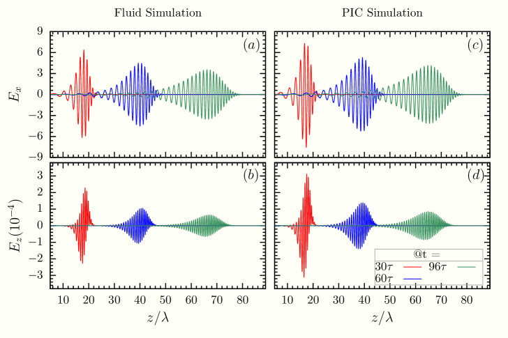
Figure 1: The spatial profile of the electromagnetic (transverse) fields (a,c) and electrostatic (longitudinal) fields (b,d) is presented at different time instances using fluid simulation (left panel) and PIC simulation (right panel). Here, we modeled the interaction of the 800 nm, 3 cycles (FWHM) Gaussian laser pulse ($a_{0}=0.1$) with plasma having density $0.5n_{c}$.

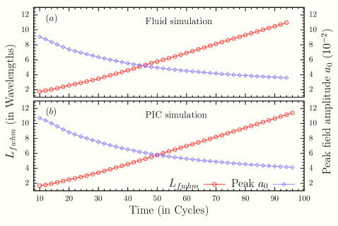
Figure 2: The temporal evolution of the pulse length (red circle, left axis) and the peak field amplitude (blue filled circles, right axis) as it propagates in the underdense plasma is compared by fluid (a) and PIC simulations (b). The pulse length $L_{fwhm}$ is estimated in units of the fundamental wavelength of the laser pulse, similarly time is presented in units of fundamental laser cycle. The laser and plasma conditions are same as Fig. 1.

The objective of this article is to study the dispersion of the electromagnetic (EM) waves as it propagates in an under-dense plasma. The propagation and the dispersion of the EM waves can be understood by the relativistic cold fluid model. Recently we developed a model to study the transition from the wakefield generation to the soliton formation Holkundkar and Brodin (2018); Brodin et al. (2006). However, for the sake of completeness here also we elaborated the cold fluid model. We have considered the immobile ions, and apart from this no further approximations are made. For detailed calculations please refer the Appendix.

The laser amplitude is normalized as $\mathbf{a}=e\mathbf{A_{\perp}}/m_{e}c$, scalar potential as $\varphi=e\phi/m_{e}c^{2}$, time and space with laser frequency and wave vector ($\omega t\rightarrow t$ and $kx\rightarrow x$) respectively, velocity as $\beta=\upsilon/c$, momentum is normalized $\mathbf{p}=\mathbf{P}/m_{e}c$, charge and mass are normalized by electron charge and mass, the electron density is normalized by critical density $n_{c}=\varepsilon_{0}\omega^{2}m_{e}/e^{2}$. By using these normalization one can easily deduce from Eq. 30-36 of the Appendix the following set of equations

$$\frac{\partial^{2}\mathbf{a}}{\partial z^{2}}-\frac{\partial^{2}\mathbf{a}}{\partial t^{2}}=n_{e}\frac{\mathbf{a}}{\gamma}$$ (1)

$$\frac{d\beta}{dt}=\frac{(1-\beta^{2})}{\gamma}\frac{\partial\varphi}{\partial z}-\frac{1}{2\gamma^{2}}\Big{(}\frac{\partial\mathbf{a}^{2}}{\partial z}+\beta\frac{\partial\mathbf{a}^{2}}{\partial t}\Big{)}$$ (2)

$$\frac{\partial n_{e}}{\partial t}+\frac{\partial}{\partial z}\Big{(}n_{e}\beta\Big{)}=0$$ (3)

$$\gamma=\sqrt{\frac{1+a^{2}}{1-\beta^{2}}}$$ (4)

$$\frac{\partial^{2}\varphi}{\partial t\partial z}=-n_{e}\beta$$ (5)

The above set of equations are the basis of our analysis of the dispersion of the EM wave in the under-dense plasma. In order to validate the results of our fluid model, we used a 1D particle-in-cell (PIC) simulation, the details of the PIC simulations are as follows: The 1D Particle-In-Cell simulation (LPIC++) Lichters et al. (1997) is carried out to compare the results of the cold fluid model. In this code the electric fields are normalized as we earlier discussed ($a_{0}=eE/m_{e}\omega c$). However space and time are taken in units of laser wavelength ($\lambda$) and one laser cycle $\tau=\lambda/c$ respectively, mass and charge are normalized with electron mass and charge respectively. We have used 100 cells per laser wavelength with each cell having 50 electron and ion macro-particles. The spatial grid size and temporal time step for the simulation are considered to be 0.01$\lambda$ and 0.01$\tau$ respectively.

III Results and Discussions

We have numerically solved the Eqs (1)-(5) in the same sequence to study the evolution of the laser pulse entering the simulation box from the left side. The simulation box of length $100$ $\lambda$ is considered, with a constant unperturbed plasma density $n_{0}$ throughout the simulation domain, the linearly polarized Gaussian laser pulse of wavelength $800$ nm has a full width half maximum (FWHM) duration of 3 cycles ($\tau_{fwhm}=3\times 2\pi$ ). The normalized amplitude $a_{0}$ is varied in the different simulations, and the boundary conditions on the left side read as:

$$\mathbf{a}(0,t)=a_{0}\exp\Big{(}-\frac{4\log(2)t^{2}}{\tau_{fwhm}^{2}}\Big{)}\cos(t)\ \ \mathbf{\hat{x}}$$ (6)

$$n_{e}(0,t)=n_{0}$$ (7)

$$\beta(0,t)=\varphi^{\prime}(0,t)=0\quad(\varphi^{\prime}\equiv\partial\varphi/\partial z).$$ (8)

It should be noted that the cold fluid relativistic model is only valid for the cases when the laser pulse amplitude is $a_{0}$ is less than unity ($a_{0}<1$) or for that matter the dispersion is in the linear regime. For ultra-intense laser pulses $a_{0}>1$ the phenomenon of the wave breaking and other non-linearities limit the applicability of the fluid approach in describing the density modulations. The results in this sections are divided in for the cases when $a_{0}<1$ wherein we compared the results of the fluid and PIC simulations along with the effects of the laser and plasma parameters on the dispersion of EM waves. On the contrary the dispersion of the ultra intense laser pulses ($a_{0}>1$) is studied by only using PIC simulations.

III.1 Pulse dispersion for $a_{0}<1$

We consider the propagation of the 800 nm, 3 cycles (FWHM), linearly polarized, Gaussian laser pulse ($a_{0}=0.1$) in the plasma with an unperturbed plasma density of $0.5n_{c}$. The spatial profiles of the transverse EM fields and longitudinal electrostatic fields are illustrated at different time instances in Fig. 1 both by using fluid simulation (left panel) as well as PIC simulations (right panel), and apparently the agreement between the two is found to be good. The dispersive nature of the laser pulse can be seen by increased pulse length and decreased peak amplitudes as estimated at different time instances. As it propagates deeper into the plasma the pulse tend to broaden. Furthermore, it can be seen from Fig. 1(b) that the wakefield or longitudinal field generation is suppressed for the chosen laser and plasma parameters and on the contrary a kind of a localized structure is co-propagating with the laser pulse [see Fig. 1(a)]. The suppression of the wakefield happens mainly when the length of the laser pulse ($c\tau_{L}$) is larger than the equivalent length of the plasma oscillations ($\upsilon_{g}\tau_{p}$), here $\upsilon_{g}$ is the group velocity of the plasma waves and $\tau_{p}$ is the duration of the one plasma cycle. In Ref. Holkundkar and Brodin (2018), we have presented the detailed analysis of the transition from the wakefield to the soliton formation.

For the same laser and plasma parameters ($a_{0}=0.1,\tau_{fwhm}=3\ \text{cycles},n_{e}=0.5n_{c}$) the time evolution of the peak field amplitude and the pulse length is presented in Fig. 2, the agreement between the fluid and PIC simulations is found to be excellent. It can be observed from Fig. 2, that the pulse length increases almost linearly with time as the pulse propagates deeper into the plasma, on the other hand, the peak field amplitudes decreases. As we discussed earlier, for this laser and plasma parameters the wakefield generation is suppressed and the modulation in plasma density actually co-moves with the laser pulse. The total energy content of the pulse is found to be almost constant during its passage in the plasma, as energy lost to the wakefield generation is almost negligible.

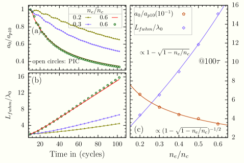
Figure 3: Temporal evolution of the peak laser amplitude (a) and pulse length (b) is presented for different plasma densities. The results of the PIC simulations are also shown with open circles in both (a) and (b). The peak amplitude is normalized to the peak value of the pulse at $t=10\tau$ ($a_{p10}$). The value of these parameters are evaluated at 100$\tau$ are also presented in (c) for different $n_{e}/n_{c}$. The $a_{0}=0.1$ and $\tau_{fwhm}=3$ cycles is considered for this case.

Next, we present the effect of the plasma density on the temporal evolution of the pulse length and the peak field amplitude of the laser pulse, during its passage to the uniform density plasma. For this we have used the same laser parameters ($a_{0}=0.1$ and $\tau_{fwhm}=3$ cycles) as in Fig. 1 and 2. The peak field amplitude is normalized to its value at $t=10\tau$ ($a_{p10}$), this has been done to iron out a slight discrepancy with PIC simulations because anyway here we are more interested in the rate change of the peak amplitude as the pulse propagates through the plasma. The constant plasma density is varied from $0.2-0.6n_{c}$. It can be observed from Fig. 3(b) that the pulse length increases linearly with time and the rate at which it increases varies with the plasma density. We have compared the results of our fluid simulation with the PIC simulation for the case with $n_{e}=0.6n_{c}$ and the agreement is found to be excellent. In Fig. 3(c) we present the pulse length and the peak amplitude as evaluated at $t=100\tau$ for different plasma densities.

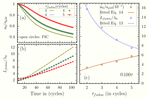
Figure 4: Temporal evolution of the peak laser amplitude (a) and pulse length (b) is presented for different pulse duration. The results of the PIC simulations are also shown with open circles in both (a) and (b). The peak amplitude is normalized to the peak value of the pulse at it would be at $t=10\tau$ ($a_{p10}$). The value of these parameters are evaluated at 100$\tau$ and are presented in (c) for different $\tau_{fwhm}$. The $a_{0}=0.1$ and $n_{e}=0.5n_{c}$ is considered for this case.

The linear broadening of the laser pulse with time can be understood in terms of the group velocity of the pulse in the plasma. In the linearized theory the group velocity (normalized to $c$) can be calculated as:

$$\upsilon_{g}=\sqrt{1-\omega_{p}^{2}/\omega^{2}}=\sqrt{1-n_{e}/n_{c}}$$ (9)

then the time evolution of pulse length ($L$) can be expected to follow the relation,

$$L(t)=L_{0}+(1-\upsilon_{g})t$$ (10)

such, that in case of vacuum ($\upsilon_{g}=1$) the pulse length remains constant, say $L_{0}$. As we have pointed out that for this cases the wakefield generation is almost suppressed and the energy content of the laser pulse is almost constant, this indicates toward the fact that as the pulse broadens, the respective peak amplitude should drop accordingly. The energy of the pulse will scale as $\propto a_{0}^{2}L$, which indicates the drop in the peak amplitude scales as $\propto 1/\sqrt{L(t)}$.

The scaling is found to be in accordance with the results presented in Fig. 3(a). Furthermore, the variation of the pulse length (as evaluated at $t=100\tau$) with the plasma density is presented in Fig. 3(c). As expected from Eq. 10, the pulse length and pulse amplitude would scale as:

$$L(n_{e})\propto 1-\sqrt{1-n_{e}/n_{c}}\quad;\quad a_{0}\propto\frac{1}{\sqrt{L(n_{e})}}$$ (11)

the fitted Eq. 11 is also illustrated in Fig. 3.

The effect of the pulse duration on the dispersion is presented in Fig. 4. Here, again we studied the time evolution of the pulse length and the peak field amplitude during the passage of the pulse through the plasma. We varied the $\tau_{fwhm}$ for fixed $a_{0}=0.1$ and $n_{e}=0.5n_{c}$. The results are also compared with the PIC simulations as well and an agreement is found to be excellent. It can be seen from Fig. 4(c) that the length of the pulse at say $t=100\tau$ decreases as we increase the laser pulse duration. It can be understood as follows, we know the shorter the pulse higher would be the bandwidth, that translates to the fact that a different portion of the pulse will propagate with the different velocity and as a result the larger broadening of the pulse. On the other hand for longer pulses the bandwidth is small, and so the associated dispersion. We can compare the time scales of the laser pulse duration with the time scales typically involved in the plasma oscillations $\tau_{fwhm}\propto 1/\omega_{p}\sim 1/\sqrt{n_{e}}$ for a rough estimates related to the dispersive nature of the plasma.

$$\tau_{fwhm}\propto\frac{1}{\sqrt{n_{e}}}$$ (12)

however, as we saw earlier the pulse length is related to the plasma density as given by Eq. 10, so in a sense $n_{e}\propto L^{2}$, this implies

$$\tau_{fwhm}\propto\frac{1}{L}\implies L\propto\frac{1}{\tau_{fwhm}}$$ (13)

and peak amplitude would be,

$$a_{0}\propto\frac{1}{\sqrt{L}}\propto\sqrt{\tau_{fwhm}}$$ (14)

Next, we further study the effect of the laser amplitude on the dispersion of the laser pulse. For this purpose we fixed the pulse duration to $\tau_{fwhm}=3$ cycles and the plasma density to $0.5n_{c}$ and varied the peak laser amplitude. The time evolution of the peak field amplitude and length of the laser pulse is presented in Fig. 5. Again as expected the linear dispersion law is found to be consistent for the laser and plasma parameters presented. Though for $a_{0}=0.3$ case, we found a bit of discrepancy with fluid simulation for pulse length evolution, otherwise the rate change of the field amplitude is consistent with the findings of the PIC simulations. The value of the field amplitude and pulse length as evaluated at $100\tau$ is also illustrated in Fig. 5(c). It is understood that high intensity laser pulses tend to disperse less as compare to the low amplitude pulses, as a consequence the pulse length of the intense pulses is smaller than then their low intensity counterpart after certain time of propagation. As we discussed earlier, the pulse length can be estimated by Eq. 10, however with the relativistic corrections the Eq. 10 is modified as,

$$L(t)=L_{0}+\Big{(}1-\sqrt{1-\frac{n_{e}}{\gamma^{\prime}n_{c}}}\Big{)}t\quad;\quad\gamma^{\prime}\equiv\sqrt{1+a_{0}^{2}}$$ (15)

here, $\gamma^{\prime}$ is relativistic factor (Eq. 4), we ignored the longitudinal motion of the electrons. The scaling of the pulse length with the initial laser amplitude is carried out using Eq. 15 and the fitted curve is also presented in Fig. 5(c).

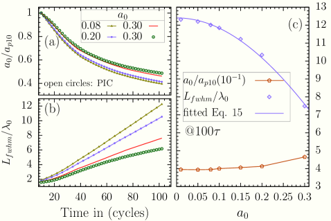
Figure 5: Temporal evolution of the peak laser amplitude (a) and pulse length (b) is presented for different laser amplitudes. The results of the PIC simulations are also shown with open circles in both (a) and (b). The peak amplitude is normalized to the peak value of the pulse at it would be at $t=10\tau$ ($a_{p10}$). The value of these parameters are evaluated at 100$\tau$ and are presented in (c) for different $a_{0}$. The $n_{e}=0.5n_{c}$ and $\tau_{fwhm}=3$ cycles is considered for this case.

III.2 Pulse dispersion for $a_{0}>1$

In the previous section, we discussed the dispersion of the laser pulses with $a_{0}<1$. We developed an analytical framework based on the cold relativistic fluid model and benchmarked the results with the 1D PIC simulations. However, for high intense laser pulses, the cold fluid model is no longer valid, as for intense laser fields the nonlinear phenomenon like wave-breaking would prevail, which indeed is outside the purview of the fluid approach. In order to study the dispersion of the intense laser pulses ($a_{0}>1$) we would be using the PIC simulations alone.

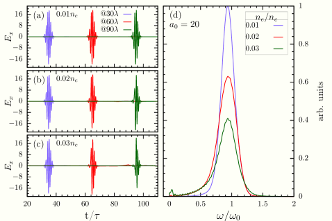
Figure 6: The temporal snapshots of the laser field as evaluated at 30, 60 and 90$\lambda$ is illustrated for the case when 3 cycle laser with $a_{0}=20$ is propagating in the plasma with density 0.01$n_{c}$ (a), 0.02$n_{c}$(b) and 0.03$n_{c}$(c). The Fourier spectrum of the laser pulse as evaluated at $90\lambda$ is also compared for different plasma densities (d).

We consider the propagation of 3 cycles ($\tau_{fwhm}$), linearly polarized, Gaussian pulse with the peak field amplitudes as $a_{0}=10,15$ and 20 in the plasma with uniform density $\lesssim 0.03n_{c}$. The reason to consider the lower plasma density (as compared to the previous section) for $a_{0}>1$ is to mitigate the formation of the overdense plasma ($n_{e}>n_{c}$) caused by the ponderomotive force exerted by intense laser pulses $a_{0}\gtrsim 10$. The overdense plasma then prohibits the further propagation of the laser pulses, till it becomes sufficiently underdense (by space-charge effect) to allow the passage of the laser pulse. For this kind of scenario we might have the reflections of the laser pulse from the different part of the plasma, where it turns overdense. In order to avoid any reflections by the formation of the overdense plasma, in this section we would be considering the plasma densities $\lesssim 0.03n_{c}$.

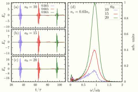
Figure 7: The temporal snapshots of the laser field as evaluated at 30, 60 and 90$\lambda$ is illustrated for the 3 cycle laser propagating in the plasma with density 0.03$n_{c}$. The laser amplitude $a_{0}=10$ (a), 15(b) and 20(c) are considered. The Fourier spectrum of the laser pulse as evaluated at $90\lambda$ is also compared for different laser amplitudes (d).

We compared the time evolution of the laser ($a_{0}=20$) electric field for three different plasma densities in Fig. 6. The field profiles are evaluated after the laser propagated the distances $30\lambda$, $60\lambda$ and $90\lambda$ in the plasma. It can be observed from this figure that the peak of the envelope moves roughly with the same velocity for different plasma densities, this indicates that the group velocity of the laser is more or less unaffected for the considered laser and plasma parameters, or maybe it would require longer simulation to see any prominent effect on propagation. We have also presented the Fourier spectrum of the laser pulse in Fig. 6(d). It can be seen that for higher densities the broadening of the frequency spectrum is larger because of the stronger plasma wave generation. The spectrum is found to be red shifted in direct correlation with the plasma density Pathak et al. (2018). The red shifting and broadening of the spectrum generally accounts for the stronger plasma wave generation, because of the energy transformation from the laser to the plasma. This fact can also be observed from the Fig. 6(d), wherein the red shift for higher density plasma is larger as compared to the lower density plasma. In order to elucidate the effect of the laser pulse amplitude on the dispersion of the laser pulse, in Fig. 7 we have varied the laser pulse amplitude while keeping the plasma density fixed at $0.03n_{c}$. The broadening of the spectrum is seen to be prominent for the $a_{0}=10$ as compare to $a_{0}=20$, because the rate at which the energy is depleted for lower laser amplitudes would be larger as compared to higher laser amplitudes.

The time evolution of the electromagnetic and electrostatic field energies are presented in Fig.8. Here, again we have considered the propagation of the 3 cycle, linearly polarized laser pulse with $a_{0}=10,20$ in the plasma having densities $0.01,0.03n_{c}$. As time progress the decrease in the electromagnetic field energy and increase in the electrostatic field energy is observed which indicates toward the stronger plasma wave generation at the cost of the electromagnetic energy. As expected it is further observed that the depletion rate of the electromagnetic field energy is larger for the laser with peak amplitude $a_{0}=10$ as compare to $a_{0}=20$. This is so because the dispersion of the high intensity laser pulses would be relatively slower than the laser pulses with lower intensity. The direct correlation of the plasma density can also be seen on the depletion rate of the electromagnetic field energy, and so the growth in the longitudinal field energy.

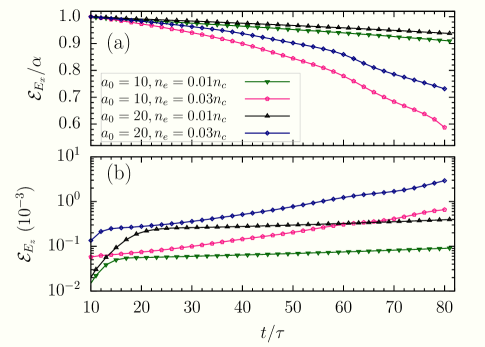
Figure 8: Temporal evolution of the laser pulse energy (a) and the longitudinal field energy is presented for 3 cycle Gaussian pulse with $a_{0}=10,\ 20$ when it propagated in the plasma with density $0.01,\ 0.03n_{c}$. The laser pulse energy in (a) is normalized to maximum value at $t=10\tau$, as we are interested in the depletion rate of the laser pulse energy for different laser and plasma parameters.

III.3 Ion acceleration by intense dispersed pulses

We have recently demonstrated the use of the negatively chirped laser pulses to accelerate the ions to a few hundreds of the MeV by using a double layer (Hydrogen plasma) target Choudhary and Holkundkar (2018). The primary layer having density $6n_{c}$ is found to be transparent for the negatively chirped laser pulse with $a_{0}=20$, creating a persistent electrostatic field which actually accelerates the ions from the secondary layer ($0.1n_{c}$). Next, we deploy the similar geometry of two layer target just after the low density plasma. The propagation of the laser pulse in underdense plasma actually causes the dispersion of the pulse, as a result the pulse would be chirped when it incidents on the two-layer target. In Fig. 9 we present the energy spectrum of the ions from the secondary layer. We considered the 3 cycle Gaussian laser pulse with $a_{0}=20$ propagates in the 100$\lambda$ long underdense plasma having density $0.03n_{c}$. The dispersed pulse then incidents on the two-layer target, first layer is $0.75\lambda$ thick with density $6n_{c}$ and adjacent secondary layer is $0.2\lambda$ thick with density $0.1n_{c}$.

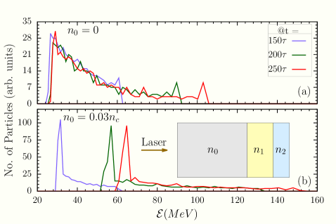
Figure 9: The energy spectrum of the ions from the secondary layer is compared when the laser directly interacts with the target i.e. $n_{0}=0$ (a) and when initially its allowed to propagate in the 100$\lambda$ pre-plasma ($n_{0}=0.03n_{c}$) prior to interaction with composite target (b). The geometry of the setup is also illustrated as an inlet. Here, $n_{0},n_{1}$ and $n_{2}$ are the plasma density of the pre-plasma, first layer and second layer respectively. Please refer the text for the physical parameters of first and second layer.

The energy spectrum of the ions from the secondary layer is compared for the cases when there is no underdense plasma and when the laser propagated through the plasma [see, Fig. 9]. It can be seen that the ions from the secondary layer are very efficiently accelerated to almost mono-energetically when the dispersed pulse interacts with the two-layer composite target geometry. The reason being the dispersion, wherein the frequency of the pulse undergone the modulation in space and time, in other words pulse is somewhat chirped. As the high frequency component of the pulse interacts with the primary layer, it transmits through the layer by the relativistic self induced transparency, or in other words, the critical density for the transmission gets modified for the chirped laser pulses. The transmitted pulse drags the electrons from the primary (as well as secondary) layer with them, creating very persistent longitudinal electrostatic field Choudhary and Holkundkar (2018). The electrostatic field then pulls the ions from the secondary layer, forming the mono-energetic ion bunch. However, in the absence of the pre-plasma the primary target is opaque to the incident unchirped pulse, resulting in the reflection. If the laser pulse suffers the reflection at the primary layer then acceleration is mostly caused by the radiation pressure mechanism, resulting in lower energy yield for the same laser intensity [see, Fig. 9(a)]. The optimization of the degree of the pulse chirping (dispersion) by varying the pre-plasma length and/or density for most efficient acceleration of the ions from the secondary layer is beyond the scope of the current manuscript.

IV Concluding Remarks

We have studied the dispersion of the laser pulse as it propagates in the underdense plasma. For the moderate laser intensities ($a_{0}<1$) we invoked a 1D relativistic cold fluid model to evaluate the spatial and temporal evolution of the laser as it propagates in the plasma with density $\lesssim 0.6n_{c}$. Apart from the immobile ions, no further approximations are made. The effect of the laser pulse amplitude, pulse duration and the plasma density is explored using the fluid model and the results are compared with the 1D PIC simulations along with the expected scaling laws. The agreement between fluid model and the PIC simulations are found to be excellent. Furthermore, in order to study the interaction of highly intense laser pulses $a_{0}\gtrsim 10$, we only relied on the PIC simulations as the nonlinear nature of the interaction process is beyond the validity of the cold relativistic fluid model. For these cases we restricted to the plasma density $\lesssim 0.03n_{c}$, or the strong ponderomotive force of laser pulses tend to make plasma over-dense ($n_{e}>n_{c}$) restricting the further propagation of the laser pulse. The conversion from the electromagnetic field energy to the electrostatic fields in the form of plasma waves results in the dispersion and so the red shift of the pump laser pulses. The dispersed pulse then allowed to be incident on the sub-wavelength two layer composite target. The ions from the thin, low density secondary layer are found to be mono-energetically accelerated to $\sim 70$ MeV, which was not the case without the dispersion.

Appendix-I

Maxwell’s equation using Coulomb gauge can be written as [J D Jackson, Classical Electrodynamics],

$$\nabla^{2}\phi=-\rho/\varepsilon_{0}$$ (16)

$$\nabla^{2}\mathbf{A}-\frac{1}{c^{2}}\frac{\partial^{2}\mathbf{A}}{\partial t^{2}}=-\mu_{0}\mathbf{J}+\frac{1}{c^{2}}\nabla\Big{(}\frac{\partial\phi}{\partial t}\Big{)}$$ (17)

We are considering the 1D case so that the variation of $\phi$ and $\mathbf{A}$ along $x$ and $y$ are not considered. The electron current density can be written as $\mathbf{J}=-en_{e}\mathbf{v}$. Furthermore, $\mathbf{v}=\mathbf{v}_{||}+\mathbf{v}_{\perp}$ and $\mathbf{v_{z}}\equiv\mathbf{v}_{||}$. By using these approximations above equations can be written as,

$$\frac{\partial^{2}\phi}{\partial z^{2}}=-\rho/\varepsilon_{0}$$ (18)

$$\frac{\partial^{2}\mathbf{A}}{\partial z^{2}}-\frac{1}{c^{2}}\frac{\partial^{2}\mathbf{A}}{\partial t^{2}}=\mu_{0}en_{e}(\mathbf{v}_{z}+\mathbf{v}_{\perp})+\frac{1}{c^{2}}\frac{\partial}{\partial z}\Big{(}\frac{\partial\phi}{\partial t}\Big{)}$$ (19)

The last equation can be split into two parts, one for perpendicular and another for parallel directions respectively. It should be noted that here parallel and perpendicular directions are taken with respect to the direction of laser pulse propagation. A Laser is polarized in a plane perpendicular to $z$ axis and hence it will contribute toward the perpendicular component of the particle velocities ($\mathbf{v}_{\perp}$). On the other hand the electrostatic potential created would be responsible for the motion of the particle along the $z$ direction. By equating the perpendicular and parallel component from RHS and LHS one obtains,

$$\frac{\partial^{2}\mathbf{A}}{\partial z^{2}}-\frac{1}{c^{2}}\frac{\partial^{2}\mathbf{A}}{\partial t^{2}}=\mu_{0}en_{e}\mathbf{v}_{\perp}$$ (20)

$$\frac{1}{c^{2}}\frac{\partial^{2}\phi}{\partial t\partial z}=-\mu_{0}en_{e}\upsilon_{z}$$ (21)

here we have used $\mathbf{v_{z}}=\upsilon_{z}\mathbf{e_{z}}$

A Laser is considered to be propagating along the $z$ direction and hence denoted by,

$$\mathbf{A}=A_{x}\mathbf{e_{x}}+A_{y}\mathbf{e_{y}}$$ (22)

here $\mathbf{e_{x}}$ and $\mathbf{e_{y}}$ are unit vectors along $x$ and $y$ directions respectively. The electric and magnetic fields are denoted by, $\mathbf{E}=-\nabla\phi-\partial\mathbf{A}/\partial t$ , and $\mathbf{B}=\nabla\times\mathbf{A}$. The electric field can further be written as, $\mathbf{E}_{||}=-\nabla\phi$ (Wakefield) and $\mathbf{E}_{\perp}=-\partial\mathbf{A}/\partial t$ (Laser electric field).

Now consider the Lorentz force equation,

$$\frac{d\mathbf{P}}{dt}=-e\Big{[}-\nabla\phi-\frac{\partial\mathbf{A}}{\partial t}+\mathbf{v\times(\nabla\times\mathbf{A})}\Big{]}$$ (23)

It should be noted that $\mathbf{A}$ only varies along $z$ direction and only contains the perpendicular components and hence $\partial_{x}=\partial_{y}=A_{z}=0$. The above equation can be written as,

$$\mathbf{v\times(\nabla\times A)}=-\upsilon_{z}\frac{\partial\mathbf{A_{\perp}}}{\partial z}+\Big{(}\mathbf{v_{\perp}}\cdot\frac{\partial\mathbf{A_{\perp}}}{\partial z}\Big{)}\mathbf{e_{z}}$$ (24)

and hence, the perpendicular and parallel component of the Lorentz force equation respectively can be written as

$$\frac{d\mathbf{P_{\perp}}}{dt}=e\Big{[}\frac{\partial}{\partial t}+\upsilon_{z}\frac{\partial}{\partial z}\Big{]}\mathbf{A_{\perp}}=\frac{d}{dt}(e\mathbf{A_{\perp}})$$ (25)

$$\frac{d\mathbf{P_{z}}}{dt}=e\frac{\partial\phi}{\partial z}\mathbf{e_{z}}-e\Big{(}\mathbf{v_{\perp}}\cdot\frac{\partial\mathbf{A_{\perp}}}{\partial z}\Big{)}\mathbf{e_{z}}$$ (26)

which translates to the fact that,

$$\mathbf{P_{\perp}}=e\mathbf{A_{\perp}}\implies\mathbf{v_{\perp}}=e\mathbf{A_{\perp}}/\gamma m_{e}$$ (27)

Substituting the value of $\mathbf{v_{\perp}}$ from (25) to (26) one obtains (we omit the $\mathbf{e_{z}}$ for the sake of convenience, as all the quantities are along $z$ direction only),

$$\frac{dP_{z}}{dt}=e\frac{\partial\phi}{\partial z}-\frac{e^{2}}{2\gamma m_{e}}\frac{\partial\mathbf{A}_{\perp}^{2}}{\partial z}$$ (28)

The last term in (28) is the Ponderomotive force which is responsible for the displacement of the electrons from the laser focus.

We need to solve for the $\upsilon_{z}$ so in view of this (28) can further be written as,

$$\frac{dP_{z}}{dt}=\frac{d}{dt}(\gamma m_{e}\upsilon_{z})=e\frac{\partial\phi}{\partial z}-\frac{e^{2}}{2\gamma m_{e}}\frac{\partial\mathbf{A}_{\perp}^{2}}{\partial z}$$ (29)

$$\gamma\frac{d\upsilon_{z}}{dt}+\upsilon_{z}\frac{d\gamma}{dt}=\frac{e}{m_{e}}\frac{\partial\phi}{\partial z}-\frac{e^{2}}{2\gamma m_{e}^{2}}\frac{\partial\mathbf{A}_{\perp}^{2}}{\partial z}$$ (30)

$$\frac{d\upsilon_{z}}{dt}=\frac{e}{\gamma m_{e}}\frac{\partial\phi}{\partial z}-\frac{e^{2}}{2\gamma^{2}m_{e}^{2}}\frac{\partial\mathbf{A}_{\perp}^{2}}{\partial z}-\frac{\upsilon_{z}}{\gamma}\frac{d\gamma}{dt}$$ (31)

The rate of change of total energy ($\mathcal{E}=\gamma mc^{2}$ ) of the charge particle can be written as,

$$\frac{d\mathcal{E}}{dt}=q\mathbf{v}\cdot\mathbf{E}$$ (32)

which in our case ($q=-e$, $m=m_{e}$ and $\mathbf{E}=-\nabla\phi-\partial\mathbf{A}/\partial t$) can be written as,

$$\frac{d\gamma}{dt}=\frac{-e}{m_{e}c^{2}}(\mathbf{v_{\perp}}+\mathbf{v_{z}})\cdot(-\nabla\phi-\partial\mathbf{A}/\partial t)$$ (33)

$$\frac{d\gamma}{dt}=\frac{e}{m_{e}c^{2}}\Big{(}\upsilon_{z}\frac{\partial\phi}{\partial z}+\mathbf{v_{\perp}}\cdot\frac{\partial\mathbf{A}_{\perp}}{\partial t}\Big{)}$$ (34)

Using again the value of $\mathbf{v_{\perp}}$ from (25) in above equation simplifies to,

$$\frac{d\gamma}{dt}=\frac{e}{m_{e}c^{2}}\Big{(}\upsilon_{z}\frac{\partial\phi}{\partial z}+\frac{e}{2\gamma m_{e}}\frac{\partial\mathbf{A}^{2}_{\perp}}{\partial t}\Big{)}$$ (35)

Substituting (35) in (31) one obtains,

$$\frac{d\upsilon_{z}}{dt}=\frac{e}{\gamma m_{e}}\Big{(}1-\frac{\upsilon_{z}^{2}}{c^{2}}\Big{)}\frac{\partial\phi}{\partial z}-\frac{e^{2}}{2\gamma^{2}m_{e}^{2}}\Big{(}\frac{\partial\mathbf{A}_{\perp}^{2}}{\partial z}+\frac{\upsilon_{z}}{c^{2}}\frac{\partial\mathbf{A}_{\perp}^{2}}{\partial t}\Big{)}$$ (36)

Local charge separation results in electrostatic fields which can be taken into account by Poisson’s equation,

$$\nabla^{2}\phi=-\frac{e}{\varepsilon_{0}}(Zn_{i}-n_{e})$$ (37)

here $Z$ and $n_{i}$ are ion charge and density respectively, however, $n_{e}$ is electron density. In 1D case $\nabla^{2}$ is replaced by $\partial^{2}/\partial z^{2}$.

$$\frac{\partial^{2}\phi}{\partial z^{2}}=-\frac{e}{\varepsilon_{0}}(Zn_{i}-n_{e})$$ (38)

The charge is conserved by continuity equation,

$$\frac{\partial n_{e}}{\partial t}+\nabla\cdot(n_{e}\mathbf{v})=0$$ (39)

which again for 1D case can be written as,

$$\frac{\partial n_{e}}{\partial t}+\frac{\partial}{\partial z}(n_{e}\upsilon_{z})=0$$ (40)

Now we deduce the expression for $\gamma$ in terms of vector potential, By definition,

$$\gamma=\frac{1}{\sqrt{1-(\upsilon_{\perp}^{2}+\upsilon_{z}^{2})/c^{2}}}$$ (41)

$$\upsilon_{\perp}^{2}+\upsilon_{z}^{2}=c^{2}(1-1/\gamma^{2})$$ (42)

Using the fact that $\mathbf{v}_{\perp}=e\mathbf{A}_{\perp}/\gamma m_{e}$ we obtain,

$$\frac{e^{2}A_{\perp}^{2}}{\gamma^{2}m_{e}^{2}}+\upsilon_{z}^{2}=c^{2}\Big{(}1-\frac{1}{\gamma^{2}}\Big{)}$$ (43)

Solving for $\gamma$ one obtains,

$$\gamma=\sqrt{\frac{1+(eA_{\perp}/m_{e}c)^{2}}{1-\upsilon_{z}^{2}/c^{2}}}$$ (44)

So finally the complete set of equations can be summarized as follows,

$$\frac{\partial^{2}\mathbf{A}_{\perp}}{\partial z^{2}}-\frac{1}{c^{2}}\frac{\partial^{2}\mathbf{A}_{\perp}}{\partial t^{2}}=\mu_{0}en_{e}\mathbf{v}_{\perp}$$ (45)

$$\frac{1}{c^{2}}\frac{\partial^{2}\phi}{\partial t\partial z}=-\mu_{0}en_{e}\upsilon_{z}$$ (46)

$$\mathbf{P_{\perp}}=e\mathbf{A_{\perp}}\implies\mathbf{v_{\perp}}=e\mathbf{A_{\perp}}/\gamma m_{e}$$ (47)

$$\frac{d\upsilon_{z}}{dt}=\frac{e}{\gamma m_{e}}\Big{(}1-\frac{\upsilon_{z}^{2}}{c^{2}}\Big{)}\frac{\partial\phi}{\partial z}-\frac{e^{2}}{2\gamma^{2}m_{e}^{2}}\Big{(}\frac{\partial\mathbf{A}_{\perp}^{2}}{\partial z}+\frac{\upsilon_{z}}{c^{2}}\frac{\partial\mathbf{A}_{\perp}^{2}}{\partial t}\Big{)}$$ (48)

$$\frac{\partial^{2}\phi}{\partial z^{2}}=-\frac{e}{\varepsilon_{0}}(Zn_{i}-n_{e})$$ (49)

$$\frac{\partial n_{e}}{\partial t}+\frac{\partial}{\partial z}(n_{e}\upsilon_{z})=0$$ (50)

$$\gamma=\sqrt{\frac{1+(eA_{\perp}/m_{e}c)^{2}}{1-\upsilon_{z}^{2}/c^{2}}}$$ (51)

These are the complete set of equations in closed form which need to be solved numerically with appropriate boundary conditions.

References

- Mangles et al. (2004) S. P. D. Mangles, C. D. Murphy, Z. Najmudin, A. G. R. Thomas, J. L. Collier, A. E. Dangor, E. J. Divall, P. S. Foster, J. G. Gallacher, C. J. Hooker, D. A. Jaroszynski, A. J. Langley, W. B. Mori, P. A. Norreys, F. S. Tsung, R. Viskup, B. R. Walton, and K. Krushelnick, Nature 431, 535 (2004).
- Faure et al. (2004) J. Faure, Y. Glinec, A. Pukhov, S. Kiselev, S. Gordienko, E. Lefebvre, J.-P. Rousseau, F. Burgy, and V. Malka, Nature 431, 541 (2004).
- Geddes et al. (2004) C. G. R. Geddes, C. Toth, J. van Tilborg, E. Esarey, C. B. Schroeder, D. Bruhwiler, C. Nieter, J. Cary, and W. P. Leemans, Nature 431, 538 (2004).
- Snavely et al. (2000) R. A. Snavely, M. H. Key, S. P. Hatchett, T. E. Cowan, M. Roth, T. W. Phillips, M. A. Stoyer, E. A. Henry, T. C. Sangster, M. S. Singh, S. C. Wilks, A. MacKinnon, A. Offenberger, D. M. Pennington, K. Yasuike, A. B. Langdon, B. F. Lasinski, J. Johnson, M. D. Perry, and E. M. Campbell, Phys. Rev. Lett. 85, 2945 (2000).
- Passoni et al. (2010) M. Passoni, L. Bertagna, and A. Zani, New J. of Physics 12, 045012 (2010).
- Qiao et al. (2011) B. Qiao, M. Zepf, P. Gibbon, M. Borghesi, B. Dromey, S. Kar, J. Schreiber, and M. Geissler, Phys. Plasmas, 18, 043102 (2011).
- Scullion et al. (2017) C. Scullion, D. Doria, L. Romagnani, A. Sgattoni, K. Naughton, D. R. Symes, P. McKenna, A. Macchi, M. Zepf, S. Kar, and M. Borghesi, Phys. Rev. Lett. 119, 054801 (2017).
- Yin et al. (2011) L. Yin, B. J. Albright, D. Jung, R. C. Shah, S. Palaniyappan, K. J. Bowers, A. Henig, J. C. Fernández, and B. M. Hegelich, Phys. Plasmas 18, 063103 (2011).
- Weng et al. (2012) S. M. Weng, M. Murakami, P. Mulser, and Z. M. Sheng, New J. Phys. 14, 063026 (2012).
- Siminos et al. (2012) E. Siminos, M. Grech, S. Skupin, T. Schlegel, and V. T. Tikhonchuk, Phys. Rev. E 86, 056404 (2012).
- Tushentsov et al. (2001) M. Tushentsov, A. Kim, F. Cattani, D. Anderson, and M. Lisak, Phys. Rev. Lett. 87, 275002 (2001).
- Fernández et al. (2017) J. C. Fernández, D. C. Gautier, C. Huang, S. Palaniyappan, B. J. Albright, W. Bang, G. Dyer, A. Favalli, J. F. Hunter, J. Mendez, M. Roth, M. Swinhoe, P. A. Bradley, O. Deppert, M. Espy, K. Falk, N. Guler, C. Hamilton, B. M. Hegelich, D. Henzlova, K. D. Ianakiev, M. Iliev, R. P. Johnson, A. Kleinschmidt, A. S. Losko, E. McCary, M. Mocko, R. O. Nelson, R. Roycroft, M. A. S. Cordoba, V. A. Schanz, G. Schaumann, D. W. Schmidt, A. Sefkow, T. Shimada, T. N. Taddeucci, A. Tebartz, S. C. Vogel, E. Vold, G. A. Wurden, and L. Yin, Phys. Plasmas 24, 056702 (2017).
- Choudhary and Holkundkar (2016) S. Choudhary and A. R. Holkundkar, Eur. Phys. J. D 70, 234 (2016).
- Kaluza et al. (2004) M. Kaluza, J. Schreiber, M. I. K. Santala, G. D. Tsakiris, K. Eidmann, J. Meyer-ter Vehn, and K. J. Witte, Phys. Rev. Lett. 93, 045003 (2004).
- Davis et al. (2005) J. Davis, G. M. Petrov, and A. L. Velikovich, Phys. Plasmas 12, 123102 (2005).
- Sullivan et al. (1994) A. Sullivan, H. Hamster, S. P. Gordon, R. W. Falcone, and H. Nathel, Opt. Lett. 19, 1544 (1994).
- Najmudin et al. (2002) Z. Najmudin, M. Tatarakis, K. Krushelnick, E. L. Clark, V. Malka, J. Faure, and A. E. Dangor, IEEE Trans. Plasma Sci. 30, 44 (2002).
- Sprangle and Hafizi (2014) P. Sprangle and B. Hafizi, Phys. Plasmas 21, 055402 (2014).
- Chen and Sudan (1993) X. L. Chen and R. N. Sudan, Phys. Fluids B 5, 1336 (1993).
- Singh et al. (2012) D. K. Singh, J. R. Davies, G. Sarri, F. Fiuza, and L. O. Silva, Phys. Plasmas 19, 073111 (2012).
- Wilson et al. (2017) T. C. Wilson, F. Y. Li, M. Weikum, and Z. M. Sheng, Plasma Phys. Control. Fusion 59, 065002 (2017).
- Smyth et al. (2016) A. G. Smyth, G. Sarri, M. Vranic, Y. Amano, D. Doria, E. Guillaume, H. Habara, R. Heathcote, G. Hicks, Z. Najmudin, H. Nakamura, P. A. Norreys, S. Kar, L. O. Silva, K. A. Tanaka, J. Vieira, and M. Borghesi, Phys. Plasmas 23, 063121 (2016).
- Hadžievski et al. (2002) L. Hadžievski, M. S. Jovanović, M. M. Škorić, and K. Mima, Phys. Plasmas 9, 2569 (2002).
- Sánchez-Arriaga et al. (2011) G. Sánchez-Arriaga, E. Siminos, and E. Lefebvre, Plasma Phys. Control. Fusion 53, 045011 (2011).
- Pukhov et al. (2011) A. Pukhov, N. Kumar, T. Tückmantel, A. Upadhyay, K. Lotov, P. Muggli, V. Khudik, C. Siemon, and G. Shvets, Phys. Rev. Lett. 107, 145003 (2011).
- Holkundkar and Brodin (2018) A. R. Holkundkar and G. Brodin, Phys. Rev. E 97, 043204 (2018).
- Brodin et al. (2006) G. Brodin, M. Marklund, L. Stenflo, and P. K. Shukla, New J. Phys. 8, 16 (2006).
- Lichters et al. (1997) R. Lichters, R. E. W. Pfund, and J. Meyer-Ter-Vehn, MPQ Report 225 (1997).
- Pathak et al. (2018) N. Pathak, A. Zhidkov, T. Hosokai, and R. Kodama, Phys. Plasmas 25, 013119 (2018).
- Choudhary and Holkundkar (2018) S. Choudhary and A. R. Holkundkar, Phys. Plasmas 25, 103111 (2018).