Recovery of compressively sensed ultrasound images with structured Sparse Bayesian Learning

Abstract

In this paper, we consider the problem of recovering compressively sensed ultrasound images. We build on prior work, and consider a number of existing approaches that we consider to be the state-of-the-art. The methods we consider take advantage of a number of assumptions on the signals including those of temporal and spatial correlation, block structure, prior knowledge of the support, and non-Gaussianity. We conduct a series of intensive tests to quantify the performance of these methods. We find that by altering the parameters of the structured Sparse Bayesian Learning approaches considered, we can significantly improve the objective quality of the reconstructed images. The results we achieve are a significant improvement upon previously proposed reconstruction techniques. In addition, we further show that by careful choice of parameters, we can obtain near-optimal results whilst requiring only a small fraction of the computational time needed for the best reconstruction quality.

I Introduction

Ultrasound imaging is possibly the most commonly used cross-sectional medical imaging modality. It has a number of advantages over alternatives, as it is relatively cheap, can easily be made portable, non-invasive and does not make use of ionising radiation. Ultrasound can also produce “real-time” images, and it is generally considered to be safe [1].

In general, ultrasound images are formed by the transmission of short ultrasound pulses from an array of transducers (most commonly piezoelectric transducers) towards the object of interest [2]. The returning (reflected) echoes are analysed and processed in order to construct an image of the object being scanned. As with all imaging modailities, ultrasound imaging generates a significant amount of data. Therefore image compression is needed to reduce the volume of data hence reducing the bit rate, and ideally this compression should not lead to any loss in perceptual image quality. The need for storage space and transmission bandwidth, particularly that caused by the diversification of ultrasound applications and telemedicine, place significant demands on existing systems in digital radiology departments [2]. The development of new technologies, allowing for the acquisition of ever greater amounts of data, places even greater demands on data processing, transmission and storage capabilities, giving rise to a need for more efficient compression techniques. In the field of medical ultrasound, there have been several recent developments that have significantly increased the amount of data generated. These developments include scanners with the ability to produce real-time 3D (RT3D) [3] or 4D [4] image data sets. One issue with these techniques is that of low frame rates, with most scanners capable of generating only a few images per second. Whilst this is fast enough to view fetal facial expressions, it is not fast enough to view the operation of the fetal heart in detail. Although several techniques have been proposed to increase the frame rates of these methods, such as multiline transmit imaging, plane-/diverging wave imaging, and retrospective gating, acquiring data at these higher frame rates results in a loss of image quality [5, 6].

The phenomenon of growth in the amount of data being generated outstripping the growth of data processing and storage capabilities is not unique to the field of ultrasound or medical imaging in general [7]. One approach that has been proposed to deal with this growth in data is that of compressed sensing. The field of compressed sensing has grown from work by Cand s, Romberg, Tao [8], and Donoho [9] on the single measurement vector (SMV) model. Later work has shown that with the shared sparsity assumption, performance can be increased in the multiple measurement vector (MMV) model [10].

Compressed sensing leverages the concept of sparsity, which is fundamental to much of modern signal processing. The idea underlying this is that many natural signals can be represented with less data than the number of samples that would be implied by the Nyquist sampling theorem [8]. This concept is used in transform coding, for example in JPEG [11] for image coding and MPEG [12] for video coding. In transform coding approaches, the signal must first be acquired at the Nyquist rate, and then compressed, effectively wasting much of the acquired data. The method of compressed sensing allows us to reduce the rate at which we sample signals, thus avoiding the need to first sample at the Nyquist rate by combining the acquisition step with the compression step. This is achieved due to two significant differences between compressed sensing and classical sampling [13]. Firstly, rather than sampling at specific points in time as with classical sensing, compressed sensing typically consists of taking inner products between the signal and general sampling kernels. Secondly, signal reconstruction in the Shannon-Nyquist framework is done by sinc interpolation, and this takes very little computation, whereas compressed sensing signal recovery methods are typically computationally intensive. In addition, with traditional transform coding approaches, the quality of the resulting image is determined primarily by the encoder at the time of encoding, whereas with compressed sensing development of improved recovery algorithms may improve the quality of the final image. The ability of compressed sensing techniques to allow signals to be acquired at rates below the Nyquist rate may allow for an increase in the framerate of ultrasound imaging techniques by reducing the amount of data acquired.

In medical imaging. compressed sensing techniques have been successfully applied to MRI in order to reduce scan time [14]. MRI is particularly amenable to compressed sensing techniques as the images are already acquired in the Fourier domain (k-space), and therefore the primary difficulty lies in the design of appropriate sampling patterns, and does not require the development of any new hardware. MRI is also of interest as it is the other commonly used cross-sectional medical imaging modality that does not make use of ionising radiation. Although MRI is capable of greater detail than ultrasound, it is significantly more expensive, not portable, and has much slower scan times.

Typically, compressed sensing approaches make no assumption on the signals being acquired other than that of sparsity. However, it is often the case that we may have knowledge of the signal properties, and the use of this knowledge can improve the ability to reconstruct compressively sensed signals. For example, it may be the case that we expect the signals to be temporally correlated, and a method was proposed in [15] to reduce the negative effect of temporal correlation on the recovery of compressively sensed signals. In addition, we might expect the non-zero elements of a signal to cluster together, and this leads to the assumption of block structure, used in [16], and combined with the assumption of temporal correlation in [17]. Another approach is to take into account the expected statistical properties of the signals. Although a common assumption, justified by the central limit theorem is that signals are Gaussian, in recent years it has become known that some natural signals do not obey this assumption. As the primary assumption needed for the central limit theorem to be applicable is that of finite variance, it is not surprising that we find that these signals can often be modeled as $\alpha-$stable distributions, as is implied by the generalised central limit theorem [18]. These distributions have found applications in financial modeling [19] (indeed, it has been argued that the 2007-2008 financial crisis can be partially attributed to the model error caused by the assumption of Gaussianity [20]), and it has also been shown that ultrasound images can be better modeled by a symmetric $\alpha-$stable (S$\alpha$S) distribution than by a Gaussian distribution [21].

There has been significant work done on applying compressed sensing techniques to ultrasound imaging. In 2012, [22] produced a review of these attempts which suggested that they fall into four categories.

The first category consists of methods that model the object being scanned as a sparse collection of scatterers. This is perhaps the easiest form to implement with existing ultrasound hardware. [23] demonstrated an implementation of this idea, although they did note some difficulties with dealing with the sensing matrix (estimated to be 458GB for a typical problem size), which they addressed by using a powerful GPU and recomputing the entries of the sensing matrix instead of storing them. It is also worth noting that they used a discrete cosine basis, as is used in this paper (although they used a 2D DCT). Work since includes the work of [24], who modelled the acquired signals as a convolution of a point spread function and tissue reflectivity function, and improved on the reconstruction quality of previous work. The previous work of [25] combined deconvolution and CS ideas.

The second category consists of methods that take advantage of the sparsity of the raw RF data, e.g. [26] and [27]. More recent work includes the work of [28], who introduced the idea of compressed beamforming in the context of the Xampling framework, and the work of [29], which extended this work to the idea of beamforming in the frequency domain.

The third category consists of methods that take advantage of the sparsity of ultrasound images in the 2D Fourier transform domain. Several of these such as [30] and [31] adopt a Bayesian approach for the reconstruction of ultrasound images.[32] introduced a framework for the compressed sensing of medical ultrasound based on modelling data with a S$\alpha$S distribution, and an approach using the iteratively reweighted least squares (IRLS) algorithm for $\ell_{p}$ pseudonorm minimisation was proposed, with $p$ related to the the characteristic exponent of the distribution of the underlying data. This approach was further extended in [33], where it was shown that performance could be improved by taking into account knowledge of the support. Another approach using a line-by-line strategy is in [34], which made use of the correlations between each ultrasound line. It is these approaches that are most closely related to the work presented in this paper. Another 1D approach can be found in the work of [35], where an FRI based approach was used.

The final category relates to Doppler imaging, which is a problem with a somewhat different nature [36, 37].

We have previously shown that it is possible to improve the reconstruction performance by taking advantage of the non-Gaussianity, temporal and block structure of the ultrasound data [38, 39], building on the work in [34] which was the first to apply the T-MSBL method (compensating for the negative effect of temporal correlation) to the recovery of compressively sensed ultrasound images. The acquisition of medical ultrasound data in a manner suitable for compressed sensing techniques has been examined in other works, e.g. [28], and also general methods using compressed sensing for sub Nyquist analog-to-digital convertors have been developed, e.g. [40], but this is beyond the scope of this paper. Here, we build on previous work, and show that by careful selection of parameters for selected structured Sparse Bayesian Learning methods, we can significantly improve the resulting reconstruction quality. We also compare these methods to a number of existing approaches, and show that we obtain significant improvements.

The rest of this paper is organised as follows. We first introduce some technical background in section II, while in section III we introduce the methods we will be comparing. In section IV we describe the datasets used, in section V we present our results on these datasets, and in section VI we conclude the paper.

II Background

In this section, we provide a brief overview of the models and theory used for compressed sensing, as well as introducing the notation used in the paper.

II-A Notation

• $\left\|\mathbf{x}\right\|_{0}$,$\left\|\mathbf{x}\right\|_{1}$,$\left\|\mathbf{x}\right\|_{2}$ denote the $\ell_{0}$ pseudo-norm, and the $\ell_{1}$ and $\ell_{2}$ norms of the vector $\mathbf{x}$.

• $\mathbf{A}_{i.}$ denotes the $i^{th}$ row of the matrix $\mathbf{A}$, and $\mathbf{A}_{.j}$ denotes the $j^{th}$ column of the matrix $\mathbf{A}$

• $\mathbf{A}\otimes\mathbf{B}$ denotes the Kronecker product of matrices $\mathbf{A}$ and $\mathbf{B}$

II-B Models

The SMV model of compressed sensing is given by

$$\mathbf{y}=\mathbf{A}\mathbf{x}+\mathbf{v}$$ (1)

Here, $\mathbf{y}\in\mathbb{R}^{N\times 1}$ represents the observed measurements, $\mathbf{A}\in\mathbb{R}^{N\times M}$ is the measurement matrix, $\mathbf{v}\in\mathbb{R}^{N\times 1}$ is a noise vector, and $\mathbf{x}\in\mathbb{R}^{M}$ is the source vector we want to recover. In the context of ultrasound imaging, we can consider $\mathbf{x}$ to correspond to a line of the ultrasound image, with each line corresponding to a single transducer element. The elements of $\mathbf{x}$ therefore correspond to equally spaced time domain samples of the reflected echoes.

The MMV model is given by

$$\mathbf{Y}=\mathbf{A}\mathbf{X}+\mathbf{V}$$ (2)

Here, $\mathbf{Y}\in\mathbb{R}^{N\times L}$ represents the observed measurements, $\mathbf{A}\in\mathbb{R}^{N\times M}$ is the measurement (or sensing) matrix, $\mathbf{V}\in\mathbb{R}^{N\times L}$ is a noise matrix, and $\mathbf{X}\in\mathbb{R}^{M\times L}$ is the source matrix we want to recover, with each row corresponding to a possible source. In the ultrasound context, $X$ is now the entire ultrasound image, with each column of $\mathbf{X}$ corresponding to a single line of the ultrasound image. The columns of $\mathbf{X}$ are arranged such that they correspond to the spatial positions of the individual transducers.

Compressed sensing relies upon the idea of sparsity. We say that $\mathbf{x}$ is $k$-sparse if at most $k$ components of $\mathbf{x}$ are non-zero, and similarly we will say that $\mathbf{X}$ is $k$-sparse if at most $k$ rows of $\mathbf{X}$ are non-zero.

In the absence of noise, in the SMV case, it has been shown that under certain assumptions (which are satisfied with probability 1 if the entries of $\Phi$ are drawn independently from a continuous probability distribution), $2k$ measurements (i.e. $N=2k$) are sufficient to guarantee the exact recovery of $\mathbf{x}$ by finding the $x$ with the minimal number of non-zero elements such that $\Phi\mathbf{x}=\mathbf{y}$ [13], and under similar assumptions, along with the assumption that $X$ is of maximal column rank and has a sufficient number of columns, $k+1$ measurements are sufficient to recover $\mathbf{X}$ exactly by finding the $\mathbf{X}$ with the minimal number of non-zero rows such that $\mathbf{AX}=\mathbf{Y}$ [10].

However, this method of recovery is computationally expensive, as it requires searching over the possible sets of non-zero elements or columns. If we assume that there are at most $k$ non-zero elements (or rows), and assume that we start searching from the smallest possible set, then we would need to check $\mathcal{O}(M^{k})$ sets, as shown in equation

$$\sum_{j=0}^{k}\left(\begin{array}[]{c}M\\ j\end{array}\right)=\mathcal{\mathcal{O}}(M^{k})$$ (3)

It is clear that this quickly becomes unfeasible for larger values of $M$ and $k$, and hence faster approximate methods such as $\ell_{1}$ norm minimisation are used. If we assume that the entries of the sensing matrix are drawn independently from a Gaussian distribution with zero mean [41] and variance $\frac{1}{N}$, then approximately $kC\log(\frac{M}{N})$ measurements are needed to ensure that the recovery of a $k$ sparse vector will be exact (i.e. the recovery based on $\ell_{1}$ norm-minimisation will coincide with that of the recovery based on $\ell_{0}$ pseudonorm minimisation) with high probability, and similarly, that if a $k$-sparse vector provides a good approximation of $\mathbf{x}$, $kC\log(\frac{M}{N})$ are needed to ensure that the estimate of $\mathbf{x}$ recovered with $\ell_{1}$ minimisation can also be expected to provide a good approximation for $\mathbf{x}$.

III Reconstruction Methods

This section describes several methods that can be used for the reconstruction of compressively sensed signals. The methods include techniques for both the SMV and MMV cases, and take into consideration assumptions on the signals including those of temporal and spatial correlation, block structure, prior knowledge of the support, and non-Gaussianity.

III-A Temporal-Multiple Sparse Bayesian Learning & Temporal-Multiple Sparse Bayesian Learning-Mixture of Gaussians-a

The T-MSBL and T-MSBL-MoG-a algorithms for the MMV model are as described in the work of [15] and [39]. The core idea is to learn the correlation structure between the measurement vectors and compensate for it.

III-B Block Sparse Bayesian Learning-Bound Optimization

Another technique derived in a similar way to T-MSBL is the method of Block Sparse Bayesian Learning (BSBL) proposed by [16]. This method can be used to exploit the fact that the non-zero components of each sample in time (column of the image) tend to occur in clusters. This technique works on each column individually as a technique for the SMV model.

The block structure model for $\mathbf{x}$ is given by equation (4).

$$\mathbf{x}=[\underbrace{x_{1,}...x_{d_{1}}}_{\mathbf{x_{1}^{\text{T}}}},...,\underbrace{x_{d_{g-1}+1},...,x_{d_{g}}}_{\mathbf{x}_{g}^{\text{T}}}]^{\text{T}}$$ (4)

The assumption used is that each block is independent, and distributed according to a zero-mean Gaussian distribution. This gives the prior shown by equations (5) and (6).

$$p(\mathbf{x};\gamma_{i},B_{i},\forall i)\sim\mathcal{N}(\mathbf{0},\Sigma_{0})$$ (5)

$$\Sigma_{0}=\begin{bmatrix}\gamma_{1}\mathbf{B}_{1}\\ &.\\ &&.\\ &&&.\\ &&&&\gamma_{g}\mathbf{B}_{g}\end{bmatrix}$$ (6)

Here, $\mathbf{B}_{i}$ represents the correlation structure within a block, and $\gamma_{i}$ an unknown nonnegative scalar parameter that determines the sparsity level of the $i$-th block. To avoid overfitting, it is assumed that $\mathbf{B}_{i}=\mathbf{B}_{j}=\mathbf{B}\forall i,j$

In this paper, it will be assumed that the blocks all have equal length.

The learning rules are obtained by following an Expectation-Maximisation method (for details, see the work of [15]). In this paper, the BSBL-Bound Optimisation (BSBL-BO) algorithm, which is significantly faster than the Expectation-Maximisation based BSBL algorithm [42] is used. This changes only the learning rule for $\gamma_{i}$, the other learning rules remain the same.

III-C Spatio Temporal-Sparse Bayesian Learning

The ST-SBL method, proposed by [17] is combination of the block sparsity idea of the BSBL method, and the correction for temporal correlation of the T-MSBL method [17], and it works on the MMV model.

The assumption ST-SBL makes on the structure of $\mathbf{X}$ is that it has block structure as given by

$$\mathbf{X}=\left[\begin{array}[]{c}\mathbf{X}_{[1].}\\ \mathbf{X}_{[2].}\\ \vdots\\ \mathbf{X}_{[g].}\end{array}\right]$$ (7)

Where $\mathbf{X}_{[i].}\in\mathbb{R}^{d_{i}\times L}$ is the $i$-th block of $\mathbf{X}$ and $\sum_{i=1}^{g}d_{i}=N$, and it is assumed that only a few of the blocks $\mathbf{X}_{[i].}$ are non-zero. As with the BSBL-BO method, in this paper it will be assumed that the blocks are all of equal size, and therefore $d_{i}=d\forall i$. For each block, it is assumed that entries in the same row of $\mathbf{X}_{[i].}$ are correlated and that entries in the same column of $\mathbf{X}_{[i].}$ are correlated, and therefore that each block has spatiotemporal correlation.

Similarly to the other SBL based algorithms, it is assumed that each block has a Gaussian distribution as

$$p(\text{vec}(\mathbf{X}_{[i].}^{T});\gamma_{i},\mathbf{B},\mathbf{C}_{i})=\mathcal{N}(0,(\gamma_{i}\mathbf{C}_{i})\otimes B)$$ (8)

Here, $\mathbf{B}\in\mathbb{R}^{L\times L}$ is an unknown positive definite matrix that captures the correlation structure in each row of $\mathbf{X}_{[i].}$, $\mathbf{C}_{i}\in\mathbb{R}^{d\times d}$ is an unknown positive definite matrix that captures the correlation structure in each column of $\mathbf{X}_{[i].}$, and $\gamma_{i}$ is an unknown nonnegative scalar parameter that determines the sparsity level of the $i$-th block.

The distribution of $\mathbf{X}$ (assuming independence of the blocks) can be written as shown by equation (9).

$$p(\text{vec}(\mathbf{X}^{T});\mathbf{B},\{\mathbf{C}_{i},\gamma_{i}\}_{i})=\mathcal{N}(0,\Pi\otimes\mathbf{B})$$ (9)

Where $\Pi$ is a block diagonal matrix given by

$$\Pi\triangleq\left[\begin{array}[]{cccc}\gamma_{1}\mathbf{C}_{1}\\ &\gamma_{2}\mathbf{C}_{2}\\ &&\ddots\\ &&&\gamma_{g}\mathbf{C}_{g}\end{array}\right]$$ (10)

The relationship to the BSBL model is clear and indeed when $L=1$ the ST-SBL model reduces to the BSBL model.

As with BSBL and T-MSBL, the learning rules are found by following an Expectation-Maximisation algorithm. For details, see the work of [17].

Note that the implementations of both the ST-SBL and BSBL-BO algorithm use a rule to remove blocks (i.e. set them to zero) if the corresponding $\gamma_{i}$ is below a certain threshold. This is done by removing the corresponding columns of $\mathbf{A}$ and rows of $\mathbf{X}$ to produce $\tilde{\mathbf{A}}$ and $\tilde{\mathbf{X}}$ which are then used for the remainder of the process. In this paper, this threshold will be referred to as $\bar{\Gamma}$.

III-D Iterative Reweighted Least Squares with Dual Prior

It was shown by [21] that ultrasound RF echoes can be modeled using a power-law shot noise model, and it was shown by [43] that this model is related to $\alpha$-stable distributions. The IRLS approach for $\ell_{p}$ pseudonorm minimisation has been used to attempt to take advantage of this, with $p$ related to $\alpha$ [32]. This has been further extended to use knowledge of the support by [33], using the modified IRLS algorithm from the work of [44], and it is that algorithm that will be used in this paper. $p$ is related to the characteristic exponent of the underlying distribution by $p=\alpha-0.01$.

III-D1 Block IRLS

The BIRLS algorithm used in this paper is an adaptation of the IRLS algorithm, with the weights calculated by summing across each block, and no prior support information is used.

IV Compressive ultrasound simulations

IV-A Thyroid image data set

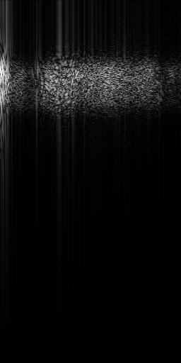
(a)

(b)

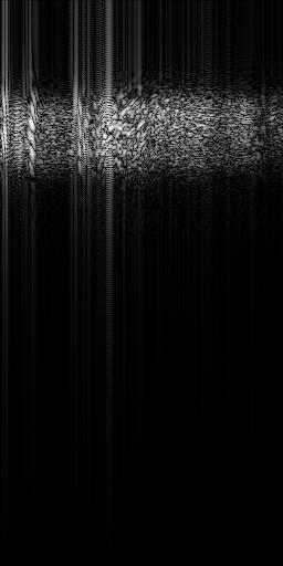
(c)

Figure 1: DCTs of images (a) 1, (b) 2 and (c) 3 from image set 1

(a)

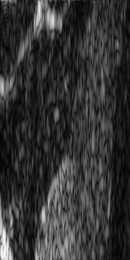
(b)

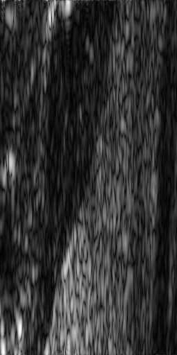
(c)

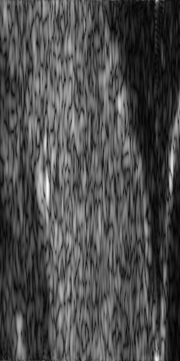
(d)

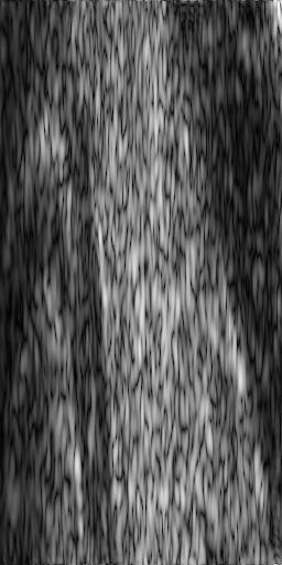
(e)

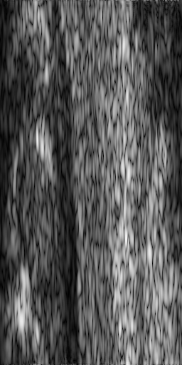
(f)

Figure 2: Ultrasound images (a) 1, (b) 2, (c) 3, (d) 4, (e) 5 and (f) 6 from set 1

The first set of images we use to test these methods come from the same dataset as those used in [33]. The data corresponds to in vivo healthy thyroid glands. The images were acquired using a Siemens Sonoline Elegra scanner using a 7.5 MHz linear probe and a sampling frequency of 50MHz. Each of the 7 images we use for testing were acquired by cropping patches of size $512\times 256$ from the original images. That is, the images consist of 256 lines, each of length 512.

We use a Discrete Cosine Transform (DCT) over a Discrete Fourier Transform (DFT) to avoid mapping the original real data to complex data which results in essentially doubling the amount of data as we would then have effectively mapped the data from $\mathbb{R}^{M}$ to $\mathbb{C^{M}}$ before applying the sensing matrix to it, which is equivalent to a mapping from $\mathbb{R}^{M}$ to $\mathbb{R}^{2M}$. It is possible to take this into account by halving the sampling rate and then taking into account the conjugate symmetry of a DFT of real data whilst recovering the original signal, but this adds a layer of unnecessary complexity. It is for similar reasons that the DCT is used in preference to the DFT in several compression standards such as JPEG. Although it is common to use 2D DCT or wavelet transforms for compressed sensing of images, this relates to the use of a CCD to capture the images, and as a CCD is a 2D array of sensors, this approach is useful. However, for ultrasound, each ultrasound line corresponds to a single transducer, and so a line by line approach provides a more practical approach. Using a line-by-line approach also has the advantage that the reconstruction of each line can be handled independently, and so parallelisation is trivial. In addition, if we wish to compressively sense an $M\times M$ image, and we assume that the number of measurements we need is a constant fraction of the number of pixels in the image, then compressively sensing the entire image at once requires a sensing matrix with $\mathcal{O}(M^{4})$ entries, whereas the line by line approach requires a sensing matrix with only $\mathcal{O}(M^{2})$ entries. Figure 1 shows the DCTs of image 1, 2, and 3 with logarithmic compression to better highlight the locations of the non-zero elements. This shows us that the assumption of sparsity in the frequency (DCT) domain is reasonable and is therefore likely to lead to good results.

To simulate a compressive sampling system, we take the DCT of each line of the image, and then project this onto a random Gaussian basis at two levels, 33% subsampling and 50% subsampling, corresponding to $\mathbf{A}\in\mathbb{R}^{171\times 512}$ and $\mathbf{A}\in\mathbb{R}^{256\times 512}$.

This simulation of the sensing system is as follows:

1. The DCT of each line (prior to envelope detection/logarithmic compression being applied) of the original ultrasound data is calculated

2. Each of these DCTs is multiplied by the sensing matrix $\mathbf{A}$

3. The CS reconstruction methods are applied to recover these DCTs

4. The inverse DCT is then applied to each of the recovered lines

5. Envelope Detection/Logarithmic compression is then applied

Note that the signals we sense are the raw ultrasound data and not the displayed image. The displayed (B-mode) images are the images we use to calculate the PSNR. These are created by taking the Hilbert transform of the original data, adding this to the original data as the complex component, taking the absolute value, logarithmically compressing this and finally rescaling such that the smallest value correspond to black (zero) and the largest value corresponds to white (one).

IV-B Brno dataset

The final set of tests are on a set of 84 images from the Signal processing laboratory of the Brno University of Technology. The description of the dataset given is reproduced for reference below.

The database contains images of common carotid artery (CCA) of ten volunteers (mean age 27.5 ± 3.5 years) with different weight (mean weight 76.5 ± 9.7 kg). Images (usually eight images per volunteer) were acquired with Sonix OP ultrasound scanner with different set-up of depth, gain, time gain compensation (TGC) curve and different linear array transducers. The image database contains 84 B-mode ultrasound images of CCA in longitudinal section. The resolution of images is approximately 390x330px. The exact resolution depends on the set-up of the ultrasound scanner. Two different linear array transducers with different frequencies (10MHz and 14MHz) were used. These frequencies were chosen because of their suitability for superficial organs imaging. All images were taken by the specialists with five year experience with scanning of arteries. Images were captured in accordance to the standard protocol with patients lying in the supine position and with the neck rotated to the left side while the right CCA was examined.

It should be noted that these images, unlike those in the first data set are provided after envelope detection and logarithmic compression, and hence any differences in the results when compared to those in the previous data set must be examined with this in mind. Before being used to test the algorithms, the images were cropped such that the height was a multiple of 32 and the width a multiple of 4. The simulated sensing system works as it did in the previous section, except that the envelope detection and logarithmic compression steps are skipped.

V Results

In this section, we conduct intensive tests in order to quantify the performance of the various methods described in section III. In order to evaluate the performance of the algorithms, we calculate the PSNR of the recovered images. The PSNR is given by equation (11).

$$\text{PSNR}(\hat{I},I)=20\log_{10}(\text{MA$X_{I}$})-10\log_{10}(\text{MSE}(\hat{I},I)$$ (11)

Here, $\text{MAX}_{I}$ is the maximum possible pixel value in the image.

In this section, ST-SBL $x/y$ refers to ST-SBL using a block size of $y$ and processing columns in blocks of size $x$, and BSBL-BO $x$ refers to BSBL-BO using a blocksize of $x$.

V-A Thyroid dataset

We first consider the effect of block size on the performance of the BSBL-BO method, fixing the pruning parameter $\bar{\Gamma}$ to be $10^{-8}$. The block size can be thought of as the size we expect clusters of non-zero elements in the DCT of each line of the ultrasound image to be. We consider only the case where all block sizes are equal, and therefore all block sizes we consider are powers of 2. In fact, we tested all such block sizes, but present only the most relevant results. In this case, we can see from Table I that at a subsampling rate of $33\%$, a block size of 32 provides optimal recovery for all images, whereas for a subsampling rate of $50\%$ we can see from Table II that although a block size of 32 is still optimal for most of the images, a block size of $64$ now provides better results for some of the images. This is slightly surprising, as we would expect the block structure to be a property of the image being reconstructed, and not of the sampling method.

We now consider the effect of block size for ST-SBL, along with considering the effect of the number of columns processed at a time. As with block size, we only consider processing the columns in blocks of equal size, and therefore all column block sizes we consider are powers of 2. As with BSBL-BO, we tested all such block sizes and column block sizes, but present only the most relevant results. ST-SBL works on the assumption of shared sparsity between columns, and we can therefore think of the column block size as representing how fast we expect the sparsity structure to change as we move between the DCTs of each line of the ultrasound image, with smaller column block sizes corresponding to faster changes. In this case, we can see from Table III that at a 33% subsampling rate, the optimal block size is typically $32$, which is consistent with the results we obtained for BSBL-BO and the optimal column block size is typically 1. For the images that deviate from this, these parameters would still be close to optimum, with a maximum loss in term of PSNR of $0.23$dB. Moving to a subsampling rate of $50\%$, these parameters become optimal for all images.

Note that with $L=1$ ST-SBL reduces to the BSBL case, and so the small difference observed between these methods is due to BSBL being implemented with a bound optimization method and ST-SBL with an expectation-maximization method, although there may also be other slight differences between the implementations.

We now consider the effect of the pruning parameter $\bar{\Gamma}$. This parameter controls when blocks are pruned, that is, at what level blocks are assumed to be zero. It can be thought of as relating to how small (in terms of the sum of squares of the block) we expect a block to be before it no longer has a significant effect on the quality of the recovered image.

For BSBL-BO, we can see from Table V that decreasing $\bar{\Gamma}$ to $2.22\times 10^{-16}$ results at the 33% subsampling levels in a slight increase in performance, but does not change the optimal block size. The pattern is repeated at the $50\%$ subsampling level, with Table VI showing a greater increase in performance than at the 33% subsampling level, but no change in optimal block size.

For ST-SBL, decreasing $\bar{\Gamma}$ to $2.22\times 10^{-16}$ results at the 33% subsampling level in no change in performance (results are not shown as they are identical to those in Table III). At a 50% subsampling rate, Table VII shows an increase in performance, but no change in optimal block size or column block size. These results are consistent with results seen with BSBL-BO.

	Block Size
Image	16	32	64
1	43.46	43.96	41.86
2	35.59	36.57	33.76
3	35.65	35.86	31.91
4	39.48	39.86	37.00
5	37.04	37.41	34.80
6	38.76	39.11	36.25
7	35.01	43.44	40.95

?tablename? I: Results for BSBL-BO (PSNR) at a 33% subsampling rate ($\bar{\Gamma}=10^{-8}$)

	Block Size
Image	16	32	64
1	34.95	47.43	50.39
2	42.42	44.16	35.00
3	42.65	31.52	42.90
4	46.45	47.47	45.32
5	44.97	46.26	44.72
6	45.92	46.94	45.53
7	35.52	49.59	50.29

?tablename? II: Results for BSBL-BO (PSNR) at a 50% subsampling rate ($\bar{\Gamma}=10^{-8}$)

Column block size	1		2		4
Block Size	16	32	16	32	16	32
Image 1	43.58	44.03	43.80	44.00	43.92	43.76
Image 2	35.56	36.62	35.80	36.28	34.47	35.11
Image 3	35.58	35.35	35.48	35.49	33.92	34.07
Image 4	39.62	39.94	39.94	39.72	39.81	39.34
Image 5	37.54	37.49	37.72	37.37	37.61	36.93
Image 6	39.00	39.34	39.14	39.34	39.04	38.96
Image 7	43.25	43.52	43.44	43.44	43.57	43.48

?tablename? III: Results for ST-SBL (PSNR) at a 33% subsampling rate ($\bar{\Gamma}=10^{-8}$)

Column block size	1		2		4
Block Size	16	32	16	32	16	32
Image 1	52.42	52.85	52.61	52.98	52.57	52.78
Image 2	44.22	45.91	43.29	44.55	43.72	43.79
Image 3	43.85	44.84	43.96	44.67	43.32	44.15
Image 4	48.92	49.77	49.08	49.55	49.00	49.17
Image 5	47.02	47.69	46.73	47.25	46.66	47.24
Image 6	48.91	49.59	48.55	49.08	48.73	48.84
Image 7	52.46	52.88	52.45	52.60	52.35	52.45

?tablename? IV: Results for ST-SBL (PSNR) at a 50% subsampling rate ($\bar{\Gamma}=10^{-8}$)

PSNR Block Size Image 16 32 1 43.48 43.98 2 35.67 36.49 3 35.69 35.97 4 39.64 39.93 5 37.36 37.50 6 38.88 39.24 7 35.03 43.48 ?tablename? V: Results for BSBL-BO (PSNR) at a 33% subsampling rate ($\bar{\Gamma}=2.22\times 10^{-16}$)

	Block Size
Image	16	32	64
1	34.96	45.69	52.71
2	33.13	45.19	35.16
3	43.01	31.56	44.24
4	49.18	50.01	49.23
5	47.06	48.05	47.60
6	48.87	49.45	49.00
7	35.42	50.49	52.87

?tablename? VI: Results for BSBL-BO (PSNR) at a 50% subsampling rate ($\bar{\Gamma}=2.22\times 10^{-16}$)

Column block size	1		2		4
Block Size	16	32	16	32	16	32
Image 1	52.75	53.27	52.75	53.13	52.69	52.91
Image 2	44.32	46.07	43.41	44.75	43.77	43.81
Image 3	43.89	44.90	43.98	44.69	43.33	44.16
Image 4	49.35	50.04	49.40	49.82	49.21	49.32
Image 5	47.15	47.89	46.84	47.28	46.75	47.32
Image 6	49.41	49.80	48.84	49.17	48.49	48.95
Image 7	52.65	53.09	52.48	52.67	52.40	52.56

?tablename? VII: Results for ST-SBL (PSNR) at a 50% subsampling rate ($\bar{\Gamma}=2.22\times 10^{-16}$)

We now compare the results obtained with ST-SBL and BSBL-BO to the other methods we described in section III. Table VIII shows comparisons with a number of other methods for recovery of compressively sensed signals at a 33% subsampling rate, and Table IX for a 50% subsampling rate. Of the methods tested, IRLS dual prior consistently has the worst performance. At a subsampling rate of 33%, T-MSBL-MoG-4 outperforms T-MSBL in 6 out of 7 cases, whereas when we move to a 50% subsampling rate, T-MSBL consistently outperforms T-MSBL-MoG-4. In addition to these methods Tables VIII and IX also show the PSNR that would be achieved by taking the 86 and 128 largest elements (in absolute value) of the DCT of each ultrasound line respectively. 86 and 128 were chosen to be half the measurements taken, as all optimal methods were SMV methods, and in this case, if the vector we wish to recover is $k$-sparse, a minimum of $2k$ measurements are required. Interestingly, both ST-SBL 1/32 ($\bar{\Gamma}=2.22\times 10^{-16}$) and BSBL-BO ($\bar{\Gamma}=2.22\times 10^{-16}$) performed significantly better than this method, suggesting that methods seeking to approximate the $k$-sparse approximation may not be ideal.

	Method
Image	ST-SBL 1/32 ($\bar{\Gamma}=2.22\times 10^{-16}$)	BSBL-BO 32 ($\bar{\Gamma}=2.22\times 10^{-16}$)	IRLS - Dual prior
1	44.03	43.98	30.01
2	36.62	36.49	26.12
3	35.35	35.97	27.54
4	39.94	39.93	28.74
5	37.49	37.50	28.71
6	39.34	39.24	30.09
7	43.52	43.48	25.34

	Method
Image	T-MSBL	T-MSBL-MoG-4	86-spase
1	31.11	31.53	38.11
2	26.92	26.94	34.56
3	28.34	29.78	35.91
4	29.78	29.31	36.10
5	29.92	30.75	34.58
6	31.66	32.28	36.72
7	29.05	27.64	36.58

?tablename? VIII: Comparison of recovery results at 33% subsampling level (PSNR)

	Method
Image	ST-SBL 1/32 ($\bar{\Gamma}=2.22\times 10^{-16}$)	BSBL-BO 32 ($\bar{\Gamma}=2.22\times 10^{-16}$)	IRLS - Dual prior
1	53.27	45.69	33.43
2	46.07	45.19	29.64
3	44.90	31.56	31.29
4	50.04	50.01	32.78
5	47.89	48.05	32.23
6	49.80	49.45	33.13
7	53.09	50.49	32.49

	Method
Image	T-MSBL	T-MSBL-MoG-4	128-sparse
1	37.44	37.31	41.80
2	32.62	30.37	38.15
3	35.25	34.94	39.26
4	34.02	34.01	39.78
5	35.87	35.84	38.69
6	38.10	37.70	40.82
7	35.27	35.12	39.73

?tablename? IX: Comparison of recovery results at 50% subsampling level (PSNR)

(a)

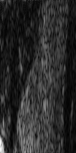
(b)

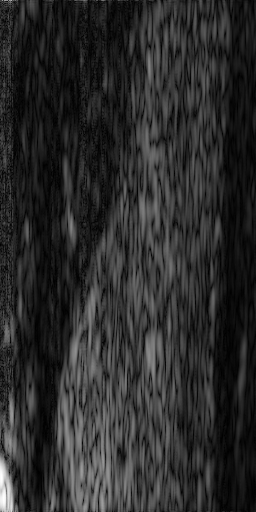
(c)

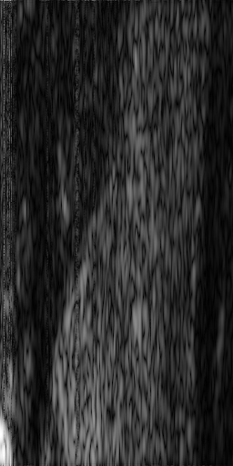
(d)

(e)

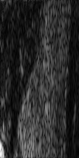
(f)

?figurename? 3: Image 1, subsampled at 50% and recovered with (a) ST-SBL 1/32 ($\bar{\Gamma}=2.22\times 10^{-16}$), (b) BSBL-BO 32 ($\bar{\Gamma}=2.22\times 10^{-16}$), (c) IRLS - Dual prior, (d) T-MSBL, (e) T-MSBL-MoG-4, (f) 128-sparse

(a)

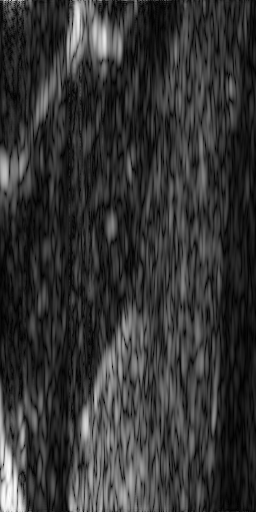
(b)

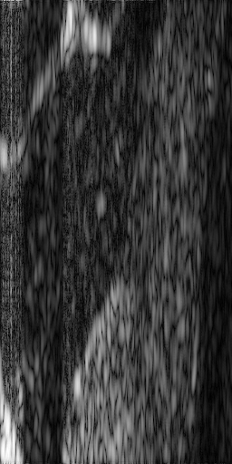
(c)

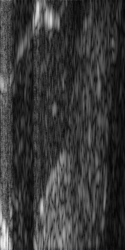
(d)

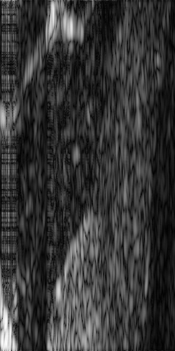
(e)

(f)

?figurename? 4: Image 2, subsampled at 33% and recovered with (a) ST-SBL 1/32 ($\bar{\Gamma}=2.22\times 10^{-16}$), (b) BSBL-BO 32 ($\bar{\Gamma}=2.22\times 10^{-16}$), (c) IRLS - Dual prior, (d) T-MSBL, (e) T-MSBL-MoG-4, (f) 86-sparse

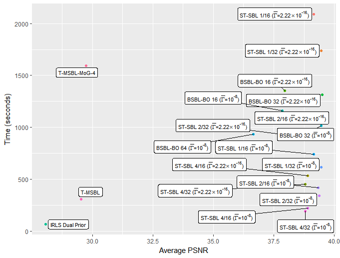
?figurename? 5: Time vs Performance for a 33% subsampling rate

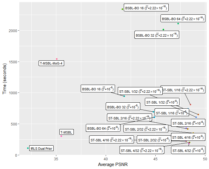
?figurename? 6: Time vs Performance for a 50% subsampling rate

Figure 3 shows Image 1 after being subsampled at 50% and then recovered with various algorithms. Figure 4 shows the same for Image 2 after it was subsampled at 33%.

Whilst we are primarily concerned with the quality of the reconstruction, the time taken for various reconstruction methods is of some practical interest. Figures 5 and 6 show plots of average time against the average PSNR achieved. For these timings, the algorithms were run using MATLAB 2014a on computer equipped with an i7-3770 processor and 8GB of RAM. Although processing more than a single column at a time with ST-SBL does not typically lead to improved recovery performance, the drop in performance is minimal, and as seen in figures 5 and 6, there is a significant reduction in computational time required by processing multiple columns at once.

Overall, the best recovery performance was achieved with ST-SBL 1/32 ($\bar{\Gamma}=2.22\times 10^{-16}$) . However, once we take the computational time into account, we would consider ST-SBL 4/32 ($\bar{\Gamma}=10^{-8}$) to be the best practical choice, as it offers only a minimal decrease in performance, and a very significant reduction in the computational time required.

A number of other methods were also tested on this set of images. The settings used for these methods are described below.

• CoSaMP, FBMP and Subspace Pursuit were fed with the “true” number of non-zero elements. This was chosen as the size of the support that was used in the IRLS Dual Prior method.

• The value of $p$ for the calculation of the weights in the BIRLS method was chosen in the same way as for IRLS.

• BIRLS and Block OMP (BOMP) were tested with block sizes of 16 and 32.

• MFOCUSS, MSBL, FOCUSS, FBMP, and $\ell$1-magic were fed with a small value ($10^{-8}$) for the noise variance.

Image	1	2	3	4	5	6	7
HTP [45]	28.52	25.13	25.74	26.70	23.97	27.62	25.99
EM-SBL [46]	28.65	25.26	26.53	28.51	27.77	29.51	26.69
FOCUSS[47]	27.75	24.62	25.98	27.43	25.38	27.65	26.43
CoSaMP [48]	16.62	15.21	15.37	14.83	13.97	13.83	16.78
Sl$0$ [49]	30.57	26.70	27.89	29.46	29.33	31.88	27.78
FBMP [50]	29.14	25.49	26.26	27.80	28.03	30.81	26.17
Subspace Pursuit [51]	28.14	24.92	24.73	24.85	22.68	28.52	25.09
ExCoV [52]	25.17	22.72	23.80	22.64	22.91	22.51	24.35
AMP [53]	29.06	25.84	27.02	28.66	27.03	29.67	27.32
BCS [54]	28.36	24.91	25.71	27.26	27.40	30.20	25.72
l1-magic [55]	29.04	25.82	27.00	28.68	27.19	29.67	27.31
BIRLS 16	38.17	34.97	35.60	36.64	38.25	40.18	36.14
BOMP 16 [56]	18.12	16.88	15.97	16.56	14.26	13.45	18.20
BIRLS 32	39.28	36.68	36.68	37.79	38.95	41.09	37.44
BOMP 32	17.76	16.24	16.48	15.81	14.44	14.49	17.47
MSBL [57]	33.12	29.13	29.67	30.66	32.77	34.65	30.01
MFOCUSS[10]	33.30	29.99	31.04	32.30	34.11	35.77	30.57

?tablename? X: Reconstruction quality of image set 2 after the DCT was subsampled at the 50% level ($\mathbf{A}\in\mathbb{R}^{171\times 512}$). Results given in terms of PSNR.

	1	2	3	4	5	6	7
HTP	21.63	19.17	19.29	19.91	18.83	20.21	20.46
EM-SBL	22.67	FAIL	FAIL	FAIL	FAIL	FAIL	FAIL
FOCUSS	22.20	20.00	20.87	21.07	20.07	20.69	21.91
CoSaMP	17.00	15.54	15.81	15.48	13.75	14.69	17.54
Sl$0$	23.17	FAIL	FAIL	FAIL	FAIL	FAIL	FAIL
FBMP	23.51	20.88	21.96	24.04	20.99	24.56	22.10
Subspace Pursuit	20.78	12.73	12.89	9.551	9.123	21.04	14.36
ExCoV	24.36	FAIL	FAIL	FAIL	FAIL	FAIL	FAIL
AMP	22.97	20.71	21.67	22.10	20.78	21.85	22.48
BCS	22.59	20.22	20.66	22.73	20.06	22.89	21.06
l1-magic	22.93	20.65	21.64	22.09	20.75	21.85	22.48
BIRLS 16	31.71	27.92	28.75	30.62	30.35	31.68	30.10
BOMP 16	17.42	15.52	15.71	16.95	16.68	16.88	18.24
BIRLS 32	32.18	28.34	29.19	31.27	30.97	32.17	30.43
BOMP 32	14.59	13.80	13.12	13.25	14.48	14.09	14.60
MSBL	29.82	26.03	27.21	28.51	28.90	31.03	28.28
MFOCUSS	30.98	27.15	28.87	29.86	30.37	32.07	28.66

?tablename? XI: Reconstruction quality of image set 2 after the DCT was subsampled at the 33% level ($\mathbf{A}\in\mathbb{R}^{256\times 512}$). Results given in terms of PSNR. FAIL indicates that the method returned only zeros.

The results of these tests can be seen in Table XI, which shows the results when the subsampling rate was 50%, and Table X which shows the results when the subsampling rate was 33%. The only method that performed sufficiently well to be of interest was BIRLS, which was the only method to outperform any of the previously tested methods. However, it was still outperformed by the previously tested methods that took advantage of block structure. This suggests that the use of the block structure assumption is able to provide significant performance gains. It is also notable that at the 33% subsampling level, some of the methods returned a vector consisting only of zeros when attempting to recover some images, and in these cases the methods are considered to have failed entirely.

However, block sparsity is clearly not a sufficient assumption in and of itself, which can be seen clearly from the dreadful performance of the BOMP method. The easiest explanation for this is that due to the nature of the method, a number of elements of the estimated vector are guaranteed to be zero, and the effect this has on performance can also be seen from the poor performance of the CoSaMP method.

Also of interest is the fact that both MFOCUSS and MSBL outperformed their SMV model counterparts. Unlike ST-SBL, these methods do not make any use of block structure. This suggests that attempting to use both block structure and joint sparsity on the signal effectively forces “too much” structure on the signal, leading to worse performance. This is in line with the poor results of BOMP, which forces some blocks to be exactly zero, whereas ST-SBL, BSBL-BO, and BIRLS all allow for solutions to be only approximately sparse.

V-B Brno dataset

Due to the large size of this test set, only a limited number of algorithms were tested. The algorithms that were chosen for testing are ST-SBL 1/32 ($\bar{\Gamma}=2.22\times 10^{-16}$), ST-SBL 4/32 ($\bar{\Gamma}=10^{-8}$), BIRLS and $\ell$1-magic

The results in terms of average PSNRand the number of times the method returned the best PSNR can be seen in Table XII for downsampling at the 33% level, and Table XIII for downsampling at the 50% level.

	Average PSNR	Number of times best method
ST-SBL 1/32 ($\bar{\Gamma}=2.22\times 10^{-16}$)	24.90	20
ST-SBL 4/32 ($\bar{\Gamma}=10^{-8}$)	25.25	59
BIRLS 32	23.46	5
$\ell$1-magic	12.47	0

Table XII: Reconstruction quality of images from set 3 after downsampling at the 33% level

	Average PSNR	Number of times best method
ST-SBL 1/32 ($\bar{\Gamma}=2.22\times 10^{-16}$)	24.96	20
ST-SBL 4/32 ($\bar{\Gamma}=10^{-8}$)	25.31	62
BIRLS 32	23.44	2
$\ell$1-magic	16.53	0

Table XIII: Reconstruction quality of images from set 3 after downsampling at the 50% level

The results are mostly as would be expected from previous results. The only unexpected item to note is that ST-SBL 4/32 ($\bar{\Gamma}=10^{-8}$) is outperforming ST-SBL 1/32 ($\bar{\Gamma}=2.22\times 10^{-16}$)) on this data set. This could be due to the signals being downsampled after envelope detection and logarithmic correction, or it could be due to the support of the DCTs of neighbouring ultrasound lines being more closely related in this set of images.

VI Conclusions

In this paper, we have thoroughly investigated what we consider to be the state-of-the-art methods for the reconstruction of compressively sensed medical ultrasound images. We have shown that by varying the parameters of structured Sparse Bayesian learning methods, we can achieve significant improvements in the recovery of compressively sensed ultrasound images. On the other hand, if we are willing to accept a slight decrease in recovery performance, we can significantly reduce the computational time required for recovery. The advantage of the structured Sparse Bayesian Learning methods is very significant, and it is worth considering why this is the case. The IRLS approach is an attempt to improve upon $\ell_{1}$ norm minimisation by more closely mimicking $\ell_{0}$ pseudonorm minimisation. However, if we examine the signals we are sensing, we see that in fact they have very few non-zero elements, and hence $\ell_{0}$ pseudonorm minimisation is unlikely to be the ideal approach. Therefore, we can conclude that this advantage comes from the previously noted ability of these methods to recover non-sparse signals [17]. Hence although it may be of some theoretical interest, development of methods which more closely approximate $\ell_{0}$ pseudonorm minimisation is unlikely to provide significant practical advantages, and efforts to improve the reconstruction of compressively sensed signals should instead focus on more accurately modeling the structure and statistical properties of the signals.

Our current work focuses on taking advantage of the statistical properties of ultrasound images in the MMV case, building on previous work [32, 33].

VII Acknowledgements

The authors would like to thank Dr Zhilin Zhang from Samsung Research America - Dallas for making his code for T-MSBL and BSBL available online, and for providing us with the code for the ST-SBL method. We would also like to thank Dr Adrian Basarab from IRIT Laboratory, Toulouse, France for providing the thyroid ultrasound images used in this study.

This work was supported in part by the Engineering and Physical Sciences Research Council (EP/I028153/1) and the University of Bristol.

- [1] C. Merritt, “Ultrasound safety: what are the issues?,” Radiology, vol. 173, no. 2, pp. 304–306, 1989.
- [2] T. L. Szabo, Diagnostic ultrasound imaging: inside out. Academic Press, 2004.
- [3] G. D. Stetten, T. Ota, C. J. Ohazama, C. Fleishman, J. Castellucci, J. Oxaal, T. Ryan, J. Kisslo, and O. v. Ramm, “Real-time 3D ultrasound: A new look at the heart,” Journal of Cardiovascular Diagnosis and Procedures, vol. 15, no. 2, pp. 73–84, 1998.
- [4] S. Yagel, S. Cohen, I. Shapiro, and D. Valsky, “3D and 4D ultrasound in fetal cardiac scanning: a new look at the fetal heart,” Ultrasound in obstetrics & gynecology, vol. 29, no. 1, pp. 81–95, 2007.
- [5] M. Cikes, L. Tong, G. R. Sutherland, and J. Dhooge, “Ultrafast cardiac ultrasound imaging: technical principles, applications, and clinical benefits,” JACC: Cardiovascular Imaging, vol. 7, no. 8, pp. 812–823, 2014.
- [6] M. Tanter and M. Fink, “Ultrafast imaging in biomedical ultrasound,” Ultrasonics, Ferroelectrics, and Frequency Control, IEEE Transactions on, vol. 61, no. 1, pp. 102–119, 2014.
- [7] R. G. Baraniuk, “More is less: signal processing and the data deluge,” Science, vol. 331, no. 6018, pp. 717–719, 2011.
- [8] E. J. Candès, J. Romberg, and T. Tao, “Robust uncertainty principles: Exact signal reconstruction from highly incomplete frequency information,” Information Theory, IEEE Transactions on, vol. 52, no. 2, pp. 489–509, 2006.
- [9] D. L. Donoho, “Compressed sensing,” Information Theory, IEEE Transactions on, vol. 52, no. 4, pp. 1289–1306, 2006.
- [10] S. F. Cotter, B. D. Rao, K. Engan, and K. Kreutz-Delgado, “Sparse solutions to linear inverse problems with multiple measurement vectors,” Signal Processing, IEEE Transactions on, vol. 53, no. 7, pp. 2477–2488, 2005.
- [11] G. K. Wallace, “The JPEG still picture compression standard,” Communications of the ACM, vol. 34, no. 4, pp. 30–44, 1991.
- [12] D. Le Gall, “MPEG: A video compression standard for multimedia applications,” Communications of the ACM, vol. 34, no. 4, pp. 46–58, 1991.
- [13] R. Baraniuk, M. A. Davenport, M. F. Duarte, and C. Hegde, “An introduction to compressive sensing,” Connexions e-textbook, 2011.
- [14] S. Vasanawala, M. Murphy, M. T. Alley, P. Lai, K. Keutzer, J. M. Pauly, and M. Lustig, “Practical parallel imaging compressed sensing MRI: Summary of two years of experience in accelerating body MRI of pediatric patients,” in Biomedical Imaging: From Nano to Macro, 2011 IEEE International Symposium on, pp. 1039–1043, IEEE, 2011.
- [15] Z. Zhang and B. D. Rao, “Sparse signal recovery with temporally correlated source vectors using sparse Bayesian learning,” Selected Topics in Signal Processing, IEEE Journal of, vol. 5, no. 5, pp. 912–926, 2011.
- [16] Z. Zhang and B. D. Rao, “Recovery of block sparse signals using the framework of block sparse Bayesian learning,” in Acoustics, Speech and Signal Processing (ICASSP), 2012 IEEE International Conference on, pp. 3345–3348, IEEE, 2012.
- [17] Z. Zhang, T.-P. Jung, S. Makeig, Z. Pi, and B. Rao, “Spatiotemporal sparse Bayesian learning with applications to compressed sensing of multichannel physiological signals,” Neural Systems and Rehabilitation Engineering, IEEE Transactions on, vol. 22, no. 6, pp. 1186–1197, 2014.
- [18] B. Gnedenko, A. Kolmogorov, B. Gnedenko, and A. Kolmogorov, “Limit distributions for sums of independent random variables,” Amer. J. Math., vol. 105, pp. 28–35, 1954.
- [19] J. Voit, The statistical mechanics of financial markets. Springer Science & Business Media, 2013.
- [20] T. Marsh and P. Pfleiderer, “"Black Swans" and the financial crisis,” Review of Pacific Basin Financial Markets and Policies, vol. 15, no. 02, p. 1250008, 2012.
- [21] M. A. Kutay, A. P. Petropulu, and C. W. Piccoli, “On modeling biomedical ultrasound RF echoes using a power-law shot-noise model,” Ultrasonics, Ferroelectrics, and Frequency Control, IEEE Transactions on, vol. 48, no. 4, pp. 953–968, 2001.
- [22] H. Liebgott, A. Basarab, D. Kouame, O. Bernard, and D. Friboulet, “Compressive sensing in medical ultrasound,” in Ultrasonics Symposium (IUS), 2012 IEEE International, pp. 1–6, IEEE, 2012.
- [23] M. F. Schiffner and G. Schmitz, “Fast pulse-echo ultrasound imaging employing compressive sensing,” in 2011 IEEE International Ultrasonics Symposium, pp. 688–691, IEEE, 2011.
- [24] Z. Chen, A. Basarab, and D. Kouamé, “Reconstruction of enhanced ultrasound images from compressed measurements using simultaneous direction method of multipliers,” arXiv preprint arXiv:1512.05586, 2015.
- [25] Z. Chen, A. Basarab, and D. Kouamé, “Compressive deconvolution in medical ultrasound imaging,” IEEE transactions on medical imaging, vol. 35, no. 3, pp. 728–737, 2016.
- [26] L. Demanet and L. Ying, “Wave atoms and sparsity of oscillatory patterns,” Applied and Computational Harmonic Analysis, vol. 23, no. 3, pp. 368–387, 2007.
- [27] H. Liebgott, R. Prost, and D. Friboulet, “Pre-beamformed rf signal reconstruction in medical ultrasound using compressive sensing,” Ultrasonics, vol. 53, no. 2, pp. 525–533, 2013.
- [28] N. Wagner, Y. C. Eldar, and Z. Friedman, “Compressed beamforming in ultrasound imaging,” Signal Processing, IEEE Transactions on, vol. 60, no. 9, pp. 4643–4657, 2012.
- [29] T. Chernyakova and Y. C. Eldar, “Fourier-domain beamforming: the path to compressed ultrasound imaging,” IEEE transactions on ultrasonics, ferroelectrics, and frequency control, vol. 61, no. 8, pp. 1252–1267, 2014.
- [30] C. Quinsac, N. Dobigeon, A. Basarab, D. Kouamé, and J.-Y. Tourneret, “Bayesian compressed sensing in ultrasound imaging,” in Computational Advances in Multi-Sensor Adaptive Processing (CAMSAP), 2011 4th IEEE International Workshop on, pp. 101–104, IEEE, 2011.
- [31] N. Dobigeon, A. Basarab, D. Kouamé, and J.-Y. Tourneret, “Regularized Bayesian compressed sensing in ultrasound imaging,” in Signal Processing Conference (EUSIPCO), 2012 Proceedings of the 20th European, pp. 2600–2604, IEEE, 2012.
- [32] A. Achim, B. Buxton, G. Tzagkarakis, and P. Tsakalides, “Compressive sensing for ultrasound RF echoes using a-stable distributions,” in Engineering in Medicine and Biology Society (EMBC), 2010 Annual International Conference of the IEEE, pp. 4304–4307, IEEE, 2010.
- [33] A. Achim, A. Basarab, G. Tzagkarakis, P. Tsakalides, and D. Kouamé, “Reconstruction of compressively sampled ultrasound images using dual prior information,” in Image Processing (ICIP), 2014 IEEE International Conference on, pp. 1283–1286, IEEE, 2014.
- [34] G. Tzagkarakis, A. Achim, P. Tsakalides, and J.-L. Starck, “Joint reconstruction of compressively sensed ultrasound RF echoes by exploiting temporal correlations,” in Biomedical Imaging (ISBI), 2013 IEEE 10th International Symposium on, pp. 632–635, IEEE, 2013.
- [35] R. Tur, Y. C. Eldar, and Z. Friedman, “Innovation rate sampling of pulse streams with application to ultrasound imaging,” IEEE Transactions on Signal Processing, vol. 59, no. 4, pp. 1827–1842, 2011.
- [36] O. Lorintiu, H. Liebgott, and D. Friboulet, “Compressed sensing doppler ultrasound reconstruction using block sparse bayesian learning,” IEEE transactions on medical imaging, vol. 35, no. 4, pp. 978–987, 2016.
- [37] S. M. Zobly and Y. M. Kakah, “Compressed sensing: Doppler ultrasound signal recovery by using non-uniform sampling & random sampling,” in Radio Science Conference (NRSC), 2011 28th National, pp. 1–9, IEEE, 2011.
- [38] R. Porter, V. B. Tadic, and A. M. Achim, “Reconstruction of compressively sensed ultrasound rf echoes by exploiting non-gaussianity and temporal structure,” in 2015 IEEE Global Conference on Image Processing (ICIP 2015), (Quebec, Canada), Sept. 2015.
- [39] R. Porter, V. Tadic, and A. Achim, “Sparse Bayesian learning for non-Gaussian sources,” Digital Signal Processing, vol. 45, pp. 2–12, 2015.
- [40] M. Mishali, Y. C. Eldar, O. Dounaevsky, and E. Shoshan, “Xampling: Analog to digital at sub-nyquist rates,” IET circuits, devices and systems, vol. 5, no. 1, pp. 8–20, 2011.
- [41] E. J. Candes, J. K. Romberg, and T. Tao, “Stable signal recovery from incomplete and inaccurate measurements,” Communications on pure and applied mathematics, vol. 59, no. 8, pp. 1207–1223, 2006.
- [42] Z. Zhang and B. D. Rao, “Extension of SBL algorithms for the recovery of block sparse signals with intra-block correlation,” IEEE Transactions on Signal Processing, vol. 61, no. 8, pp. 2009–2015, 2013.
- [43] A. P. Petropulu and J.-C. Pesquet, “Power-law shot noise and its relationship to long-memory -stable processes,” Signal Processing, IEEE Transactions on, vol. 48, no. 7, pp. 1883–1892, 2000.
- [44] C. J. Miosso, R. Von Borries, M. Argàez, L. Velázquez, C. Quintero, and C. Potes, “Compressive sensing reconstruction with prior information by iteratively reweighted least-squares,” Signal Processing, IEEE Transactions on, vol. 57, no. 6, pp. 2424–2431, 2009.
- [45] S. Foucart, “Hard thresholding pursuit: an algorithm for compressive sensing,” SIAM Journal on Numerical Analysis, vol. 49, no. 6, pp. 2543–2563, 2011.
- [46] D. P. Wipf and B. D. Rao, “Sparse Bayesian learning for basis selection,” IEEE Transactions on Signal Processing, vol. 52, no. 8, pp. 2153–2164, 2004.
- [47] I. F. Gorodnitsky and B. D. Rao, “Sparse signal reconstruction from limited data using FOCUSS: A re-weighted minimum norm algorithm,” IEEE Transactions on signal processing, vol. 45, no. 3, pp. 600–616, 1997.
- [48] D. Needell and J. A. Tropp, “Cosamp: Iterative signal recovery from incomplete and inaccurate samples,” Applied and Computational Harmonic Analysis, vol. 26, no. 3, pp. 301–321, 2009.
- [49] G. H. Mohimani, M. Babaie-Zadeh, and C. Jutten, “Fast sparse representation based on smoothed l0 norm,” in International Conference on Independent Component Analysis and Signal Separation, pp. 389–396, Springer, 2007.
- [50] P. Schniter, L. C. Potter, and J. Ziniel, “Fast Bayesian matching pursuit,” in Information Theory and Applications Workshop, 2008, pp. 326–333, IEEE, 2008.
- [51] W. Dai and O. Milenkovic, “Subspace pursuit for compressive sensing: Closing the gap between performance and complexity,” tech. rep., DTIC Document, 2008.
- [52] K. Qiu and A. Dogandzic, “Variance-component based sparse signal reconstruction and model selection,” IEEE Transactions on Signal Processing, vol. 58, no. 6, pp. 2935–2952, 2010.
- [53] D. L. Donoho, A. Maleki, and A. Montanari, “Message passing algorithms for compressed sensing: I. motivation and construction,” in Information Theory (ITW 2010, Cairo), 2010 IEEE Information Theory Workshop on, pp. 1–5, IEEE, 2010.
- [54] S. Ji, Y. Xue, and L. Carin, “Bayesian compressive sensing,” Signal Processing, IEEE Transactions on, vol. 56, no. 6, pp. 2346–2356, 2008.
- [55] E. Candes and J. Romberg, “l1-magic: Recovery of sparse signals via convex programming,” URL: www.acm.caltech.edu/l1magic/downloads/l1magic.pdf, vol. 4, p. 14, 2005.
- [56] Y. C. Eldar, P. Kuppinger, and H. Bolcskei, “Block-sparse signals: Uncertainty relations and efficient recovery,” IEEE Transactions on Signal Processing, vol. 58, no. 6, pp. 3042–3054, 2010.
- [57] D. P. Wipf and B. D. Rao, “An empirical Bayesian strategy for solving the simultaneous sparse approximation problem,” Signal Processing, IEEE Transactions on, vol. 55, no. 7, pp. 3704–3716, 2007.