Automaticity and invariant measures
of linear cellular automata

Abstract.

We show that spacetime diagrams of linear cellular automata $\Phi:\mathbb{F}_{p}^{\mathbb{Z}}\to\mathbb{F}_{p}^{\mathbb{Z}}$ with $(-p)$-automatic initial conditions are automatic. This extends existing results on initial conditions which are eventually constant. Each automatic spacetime diagram defines a $(\sigma,\Phi)$-invariant subset of $\mathbb{F}_{p}^{\mathbb{Z}}$, where $\sigma$ is the left shift map, and if the initial condition is not eventually periodic then this invariant set is nontrivial. For the Ledrappier cellular automaton we construct a family of nontrivial $(\sigma,\Phi)$-invariant measures on $\mathbb{F}_{3}^{\mathbb{Z}}$. Finally, given a linear cellular automaton $\Phi$, we construct a nontrivial $(\sigma,\Phi)$-invariant measure on $\mathbb{F}_{p}^{\mathbb{Z}}$ for all but finitely many $p$.

1. Introduction

In this article, we study the relationship between $p$-automatic sequences and spacetime diagrams of linear cellular automata over the finite field $\mathbb{F}_{p}$, where $p$ is prime. For definitions, see Section 2.

There are many characterisations of $p$-automatic sequences. For readers familiar with substitutions, Cobham’s theorem [18] tells us that they are codings of fixed points of length-$p$ substitutions. In an algebraic setting, Christol’s theorem tells us that they are precisely those sequences whose generating functions are algebraic over $\mathbb{F}_{p}(x)$. In [35], we characterise $p$-automatic sequences as those sequences that occur as columns of two-dimensional spacetime diagrams of linear cellular automata $\Phi:\mathbb{F}_{p}^{\mathbb{Z}}\to\mathbb{F}_{p}^{\mathbb{Z}}$, starting with an eventually periodic initial condition.

We investigate the nature of a spacetime diagram as a function of its initial condition, when the initial condition is $p$-automatic. In the special case when the initial condition is eventually $0$ in both directions and the cellular automaton has right radius $0$, this question has been thoroughly studied in a series of articles by Allouche, von Haeseler, Lange, Petersen, Peitgen, and Skordev [5, 6, 7]. Amongst other things, the authors show that an $\mathbb{N}\times\mathbb{N}$-configuration which is generated by a linear cellular automaton, whose right radius is $0$, and an eventually $0$ initial condition, is $[p,p]$-automatic. In [31], Pivato and the second author have also studied the substitutional nature of spacetime diagrams of more general cellular automata with eventually periodic initial conditions.

In Sections 3 and 4 we extend these previous results by relaxing the constraints imposed on the initial conditions and the cellular automata. We allow initial conditions to be bi-infinite $(-p)$-automatic sequences or, equivalently, concatenations of two $p$-automatic sequences. Iterating $\Phi$ produces a $\mathbb{Z}\times\mathbb{N}$-configuration, and we show in Theorem 3.10, Theorem 3.14, and Corollary 3.15, that such spacetime diagrams are automatic, with two possible definitions of automaticity: either by shearing a configuration supported on a cone or by considering $[-p,p]$-automaticity. Our results are constructive, in that given an automaton that generates an automatic initial condition, we can compute an automaton that generates the spacetime diagram. We perform such a computation in Example 3.11, which we use as a running example throughout the article. While the spacetime diagram has a substitutional nature, the alphabet size makes the computation of this substitution by hand infeasible, and indeed difficult even using software.

We can also extend a spacetime diagram backward in time to obtain a $\mathbb{Z}\times\mathbb{Z}$-configuration where each row is the image of the previous row under the action of the cellular automaton. In Lemma 4.2 we show that the initial conditions that generate a $\mathbb{Z}\times\mathbb{Z}$-configuration are supported on a finite collection of lines. In Theorem 4.5, we show that if the initial conditions are chosen to be $p$-automatic, then the resulting spacetime diagram is a concatenation of four $[p,p]$-automatic configurations.

Apart from the intrinsic interest of studying automaticity of spacetime diagrams, one motivation for our study is a search for closed nontrivial sets in $\mathbb{F}_{p}^{\mathbb{Z}}$ which are invariant under the action of both the left shift map $\sigma$ and a fixed linear cellular automaton $\Phi$. Analogously, we also search for measures $\mu$ on one-dimensional subshifts $(X,\sigma)$ that are invariant under the action of both $\sigma$ and $\Phi$.

We give a brief background. Furstenberg [22] showed that any closed subset of the unit interval $I$ which is invariant under both maps $x\mapsto 2x\bmod 1$ and $x\mapsto 3x\bmod 1$ must be either $I$ or finite. This is an example of topological rigidity. Furstenberg asked if there also exists a measure rigidity, i.e. if there exists a nontrivial measure $\mu$ on $I$ which is invariant under these same two maps. By “nontrivial” we mean that $\mu$ is neither the Lebesgue measure nor finitely supported. This question is known as the $({\times 2},{\times 3})$ problem.

The $({\times 2},{\times 3})$ problem has a symbolic interpretation, which is to find a measure on $\mathbb{F}_{2}^{\mathbb{N}}$ which is invariant under both $\sigma$, which corresponds to multiplication by $2$, and the map $u\mapsto u+\sigma(u)$, which corresponds to multiplication by $3$ and where $+$ represents addition with carry. One can ask a similar question for $\sigma$ and the Ledrappier cellular automaton $u\mapsto u+\sigma(u)$, where $+$ represents coordinate-wise addition modulo $2$. One way to produce such measures is to average iterates, under the cellular automaton, of a shift-invariant measure, and to take a limit measure. Pivato and the second author [30] show that starting with a Markov measure, this procedure only yields the Haar measure $\lambda$. Host, Maass, and Martinez [23] show that if a $(\sigma,\Phi)$-invariant measure has positive entropy for $\Phi$ and is ergodic for the shift or the $\mathbb{Z}^{2}$-action then $\mu=\lambda$. The problem of identifying which measures are $(\sigma,\Phi)$-invariant is an open problem; see for example Boyle’s survey article [14, Section 14] on open problems in symbolic dynamics or Pivato’s article [29, Section 3] on the ergodic theory of cellular automata.

In Sections 5 and 6 we apply results of Sections 3 and 4 to find $(\sigma,\Phi)$-invariant sets and measures. Spacetime diagrams generate subshifts $(X,\sigma_{1},\sigma_{2})$, where $\sigma_{1}$ and $\sigma_{2}$ are the left and down shifts, and these subshifts project to closed sets in $\mathbb{F}_{p}^{\mathbb{Z}}$ that are $(\sigma,\Phi)$-invariant. Similarly, we show in Proposition 6.1 that $(\sigma_{1},\sigma_{2})$-invariant measures on $X$ project to $(\sigma,\Phi)$-invariant measures supported on a subset of $\mathbb{F}_{p}^{\mathbb{Z}}$. Einsiedler [21] constructs, for each $s$ in the interval $0\leq s\leq 1$, a $(\sigma_{1},\sigma_{2})$-invariant set and a $(\sigma_{1},\sigma_{2})$-invariant measure whose entropy in any direction is $s$ times the maximal entropy in that direction. He builds invariant sets using intersection sets as described in Section 5.2 and asks if every $(\sigma_{1},\sigma_{2})$-invariant set is an intersection set. He also asks for the nature of the invariant measures. We show in Theorem 5.8 that each automatic spacetime diagram generates a $(\sigma,\Phi)$-invariant set of small (one-dimensional) word complexity. If we assume that the initial condition is not spatially periodic and the cellular automaton is not a shift, we show in Proposition 5.3 that these sets are nontrivial. The invariant sets we find are not obviously intersection sets.

The quest for nontrivial $(\sigma,\Phi)$-invariant measures appears to be more delicate. Let $(X_{U},\sigma_{1},\sigma_{2})$ be a subshift generated by a $[-p,-p]$-automatic configuration $U$. Theorem 6.11 states that the measures supported on such subshifts are convex combinations of measures supported on codings of substitution shifts. We show in Theorem 5.2 that $U$ has at most polynomial complexity. Therefore the $(\sigma,\Phi$)-invariant measures guaranteed by Proposition 6.1 are not the Haar measure. However they may be finitely supported: the shift $X_{U}$ generated by a nonperiodic spacetime diagram $U$ can contain periodic points on which a shift-invariant measure is supported. In Theorems 6.13 and 6.15 we identify cellular automata and nonperiodic initial conditions that yield two-dimensional shifts containing constant configurations.

We show in Corollary 6.3 that spacetime diagrams that do not contain large one-dimensional repetitions support nontrivial $(\sigma,\Phi)$-invariant measures, and in Theorem 6.2 we show that this condition is decidable. In Theorem 6.4 we show that for the Ledrappier cellular automaton there exists a family of substitutions all of whose spacetime diagrams, including our running example, support nontrivial measures. In Theorem 6.9, we generalise this last proof, showing that for any linear cellular automaton $\Phi$, nontrivial $(\sigma,\Phi)$-invariant measures exist for all but finitely many primes $p$. Given $\Phi:\mathbb{F}_{p}^{\mathbb{Z}}\rightarrow\mathbb{F}_{p}^{\mathbb{Z}}$, to what extent it is the case that a random $p$-automatic initial condition generates a nontrivial $(\sigma,\Phi)$-invariant measure? This remains open.

We are indebted to Allouche and Shallit’s classical text [4], referring to proofs therein on many occasions, which carry through in our extended setting. In Section 2, we provide a brief background on linear cellular automata, larger rings of generating functions in two variables, and $p$- and $(-p)$-automaticity. In Section 3 we prove that $\mathbb{Z}\times\mathbb{N}$-indexed spacetime diagrams are automatic if we start with automatic initial conditions. In Section 4 we extend these results to include $\mathbb{Z}\times\mathbb{Z}$-indexed spacetime diagrams. In Section 5 we show that automatic spacetime diagrams for $\Phi$ yield nontrivial $(\sigma,\Phi)$-invariant sets and discuss their relation to the intersection sets defined by Kitchens and Schmidt [25]. Finally in Section 6, we study $(\sigma,\Phi)$-invariant measures supported on automatic spacetime diagrams.

2. Preliminaries

2.1. Linear cellular automata

Let $\mathcal{A}$ be a finite alphabet. An element in $\mathcal{A}^{\mathbb{Z}}$ is called a configuration and is written $u=(u_{m})_{m\in\mathbb{Z}}$. The (left) shift map $\sigma:\mathcal{A}^{\mathbb{Z}}\rightarrow\mathcal{A}^{\mathbb{Z}}$ is the map defined as $(\sigma(u))_{m}\mathrel{\mathop{:}}=u_{m+1}$. Let $\mathcal{A}$ be endowed with the discrete topology and $\mathcal{A}^{\mathbb{Z}}$ with the product topology; then $\mathcal{A}^{\mathbb{Z}}$ is a metrisable Cantor space. A (one-dimensional) cellular automaton is a continuous, $\sigma$-commuting map $\Phi:\mathcal{A}^{\mathbb{Z}}\rightarrow\mathcal{A}^{\mathbb{Z}}$. The Curtis–Hedlund–Lyndon theorem tells us that a cellular automaton is determined by a local rule $f$: there exist integers $\ell$ and $r$ with $-\ell\leq r$ and $f:\mathcal{A}^{r+\ell+1}\to\mathcal{A}$ such that, for all $m\in\mathbb{Z}$, $(\Phi(u))_{m}=f(u_{m-\ell},\dots,u_{m+r})$. Let $\mathbb{N}$ denote the set of non-negative integers.

Definition 2.1.

Let $\Phi:\mathcal{A}^{\mathbb{Z}}\rightarrow\mathcal{A}^{\mathbb{Z}}$ be a cellular automaton and let $u\in\mathcal{A}^{\mathbb{Z}}$. If $U\in\mathcal{A}^{\mathbb{Z}\times\mathbb{N}}$ satisfies $U|_{\mathbb{Z}\times\{0\}}=u$ and $\Phi(U|_{\mathbb{Z}\times\{n\}})=U|_{\mathbb{Z}\times\{n+1\}}$ for each $n\in\mathbb{N}$, we call $U=\operatorname*{ST}_{\Phi}(u)$ the spacetime diagram generated by $\Phi$ with initial condition $u$.

For the cellular automata in this article, $\mathcal{A}=\mathbb{F}_{p}$. The configuration space $\mathbb{F}_{p}^{\mathbb{Z}}$ forms a group under componentwise addition; it is also an $\mathbb{F}_{p}$-vector space.

Definition 2.2.

A cellular automaton $\Phi:\mathbb{F}_{p}^{\mathbb{Z}}\rightarrow\mathbb{F}_{p}^{\mathbb{Z}}$ is linear if $\Phi$ is an $\mathbb{F}_{p}$-linear map, i.e. $(\Phi(u))_{m}=\alpha_{-\ell}u_{m-\ell}+\dots+\alpha_{0}u_{m}+\dots+\alpha_{r}u_{m+r}$ for some nonnegative integers $\ell$ and $r$, called the left and right radius of $\Phi$. The generating polynomial [6] of $\Phi$, denoted $\phi$, is the Laurent polynomial

$$\phi(x)\mathrel{\mathop{:}}=\alpha_{-\ell}x^{\ell}+\dots+\alpha_{0}+\dots+\alpha_{r}x^{-r}.$$

We remark that our use of $\phi$ for the generating polynomial differs from usage in the literature of $\phi$ as $\Phi$’s local rule, which is the map $(u_{m-\ell},\dots,u_{m+r})\mapsto\alpha_{-\ell}u_{m-\ell}+\dots+\alpha_{r}u_{m+r}$.

The generating polynomial has the property that $\phi(x)\sum_{m\in\mathbb{Z}}u_{m}x^{m}=\sum_{m\in\mathbb{Z}}(\Phi(u))_{m}x^{m}$. We will identify sequences $(u_{m})_{m\in\mathbb{Z}}$ with their generating function $f(x)=\sum_{m\in\mathbb{Z}}u_{m}x^{m}$. Recall that $\mathbb{F}_{p}[x]$ and $\mathbb{F}_{p}\llbracket x\rrbracket$ are the rings of polynomials and power series in the variable $x$ with coefficients in $\mathbb{F}_{p}$ respectively. Let $\mathbb{F}_{p}(x)$ and $\mathbb{F}_{p}((x))$ be their respective fields of fractions: $\mathbb{F}_{p}(x)$ is the field of rational functions and $\mathbb{F}_{p}((x))$ is that of formal Laurent series; elements of $\mathbb{F}_{p}((x))$ are expressions of the form $f(x)=\sum_{m\geq m_{0}}u_{m}x^{m}$, where $u_{m}\in\mathbb{F}_{p}$ and $m_{0}\in\mathbb{Z}$.

2.2. Cones

A cone is a subset of $\mathbb{Z}\times\mathbb{Z}$ of the form $\{\mathbf{v}_{0}+s\mathbf{v}_{1}+t\mathbf{v}_{2}:s\geq 0,t\geq 0\}$ for some $\mathbf{v}_{0},\mathbf{v}_{1},\mathbf{v}_{2}\in\mathbb{Z}\times\mathbb{Z}$ such that $\mathbf{v}_{1}$ and $\mathbf{v}_{2}$ are linearly independent. The cone generated by $\mathbf{v}_{1}$ and $\mathbf{v}_{2}$ is the cone $\{s\mathbf{v}_{1}+t\mathbf{v}_{2}:s\geq 0,t\geq 0\}$.

If a cellular automaton is begun from an initial condition $u$ satisfying $u_{m}=0$ for all $m\leq-1$, then the spacetime diagram $\operatorname*{ST}_{\Phi}(u)$ is supported on the cone generated by $(1,0)$ and $(-r,1)$. For example, see Figure 1. If $r\geq 1$ then this cone contains points with negative entries, but we would still like to represent $\operatorname*{ST}_{\Phi}(u)$ as a formal power series in some ring. We follow the geometric exposition given by Aparicio Monforte and Kauers [8].

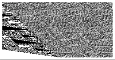
Figure 1. Spacetime diagram $\operatorname*{ST}_{\Phi}(u)$ for a cellular automaton with generating polynomial $\phi(x)=x^{-1}+x^{-3}+x^{-7}\in\mathbb{F}_{2}[x]$. The dimensions are $511\times 256$, and time goes up the page. The right half $(u_{m})_{m\geq 0}$ of the initial condition is the Thue–Morse sequence (the fixed point beginning with $0$ of $0\to 01,1\to 10$), and $u_{m}=0$ for all $m\leq-1$. By Theorem 3.5, this spacetime diagram, restricted to the cone generated by the vectors $(1,0)$ and $(-7,1)$, has an algebraic generating function.

By definition, a cone $\mathcal{C}$ is line-free, that is, for every ${\mathbf{n}}\in\mathcal{C}\setminus\{(0,0)\}$, we have $-{\mathbf{n}}\not\in\mathcal{C}$. This places us within the scope of [8].

For each cone $\mathcal{C}$, let $\mathbb{F}_{p,\mathcal{C}}\llbracket x,y\rrbracket$ be the set of all formal power series in $x$ and $y$, with coefficients in $\mathbb{F}_{p}$, whose support is in $\mathcal{C}$. Then (ordinary) multiplication of two elements in $\mathbb{F}_{p,\mathcal{C}}\llbracket x,y\rrbracket$ is well defined, and the product belongs to $\mathbb{F}_{p,\mathcal{C}}\llbracket x,y\rrbracket$; in fact $\mathbb{F}_{p,\mathcal{C}}\llbracket x,y\rrbracket$ is an integral domain [8, Theorems 10 and 11].

Let $\preceq$ be the reverse lexicographic order on $\mathbb{Z}\times\mathbb{Z}$, i.e. $(m_{1},n_{1})\preceq(m_{2},n_{2})$ if $n_{1}<n_{2}$ or if $n_{1}=n_{2}$ and $m_{1}\leq m_{2}$. A cone $\mathcal{C}$ is compatible with $\preceq$ if $(0,0)\preceq(m,n)$ for all $(m,n)\in\mathcal{C}$. Every cone contained in the set $\{(m,n):n>0\}\cup\{(m,0):m\geq 0\}$ is compatible with $\preceq$. Let

$$\mathbb{F}_{p,\preceq}\llbracket x,y\rrbracket\mathrel{\mathop{:}}=\bigcup_{\text{$\mathcal{C}$ compatible with $\preceq$}}\mathbb{F}_{p,\mathcal{C}}\llbracket x,y\rrbracket.$$

Then $\mathbb{F}_{p,\preceq}\llbracket x,y\rrbracket$ is a ring contained in the field $\bigcup_{(m,n)\in\mathbb{Z}\times\mathbb{Z}}x^{m}y^{n}\mathbb{F}_{p,\preceq}\llbracket x,y\rrbracket$  [8, Theorem 15]. This field also contains the field $\mathbb{F}_{p}(x,y)$ of rational functions. Researchers working with automatic sequences have previously worked with $\mathbb{F}_{p,\preceq}\llbracket x,y\rrbracket$ [1, 3].

2.3. Automatic initial conditions

Next we define automatic sequences, which we will use as initial conditions for spacetime diagrams.

Definition 2.3.

A deterministic finite automaton with output (DFAO) is a $6$-tuple $(\mathcal{S},\Sigma,\delta,s_{0},\mathcal{A},\omega)$, where $\mathcal{S}$ is a finite set (of states), $s_{0}\in\mathcal{S}$ (the initial state), $\Sigma$ is a finite alphabet (the input alphabet), $\mathcal{A}$ is a finite alphabet (the output alphabet), $\omega:\mathcal{S}\rightarrow\mathcal{A}$ (the output function), and $\delta:\mathcal{S}\times\Sigma\rightarrow\mathcal{S}$ (the transition function).

In this article, our output alphabet is $\mathcal{A}=\mathbb{F}_{p}$.

The function $\delta$ extends in a natural way to the domain $\mathcal{S}\times\Sigma^{*}$, where $\Sigma^{*}$ is the set of all finite words on the alphabet $\Sigma$. Namely, define $\delta(s,m_{\ell}\cdots m_{1}m_{0})\mathrel{\mathop{:}}=\delta(\delta(s,m_{0}),m_{\ell}\cdots m_{1})$ recursively. If $\Sigma=\{0,\dots,p-1\}$, this allows us to feed the standard base-$p$ representation $m_{\ell}\cdots m_{1}m_{0}$ of an integer $m$ into an automaton, beginning with the least significant digit. (Recall that the standard base-$p$ representation of $0$ is the empty word.) All automata in this article process integers by reading their least significant digit first.

A sequence $(u_{m})_{m\geq 0}$ of elements in $\mathbb{F}_{p}$ is $p$-automatic if there is a DFAO $(\mathcal{S},\{0,\dots,p-1\},\delta,s_{0},\mathbb{F}_{p},\omega)$ such that $u_{m}=\omega(\delta(s_{0},m_{\ell}\cdots m_{1}m_{0}))$ for all $m\geq 0$, where $m_{\ell}\cdots m_{1}m_{0}$ is the standard base-$p$ representation of $m$.

Similarly, we say that a sequence $(U_{m,n})_{(m,n)\in\mathbb{N}\times\mathbb{N}}$ is $[p,p]$-automatic if there is a DFAO $(\mathcal{S},\{0,\dots,p-1\}^{2},\delta,s_{0},\mathbb{F}_{p},\omega)$ such that

$$U_{m,n}=\omega(\delta(s_{0},(m_{\ell},n_{\ell})\cdots(m_{1},n_{1})(m_{0},n_{0})))$$

for all $(m,n)\in\mathbb{N}\times\mathbb{N}$, where $m_{\ell}\cdots m_{1}m_{0}$ is a base-$p$ representation of $m$ and $n_{\ell}\cdots n_{1}n_{0}$ is a base-$p$ representation of $n$. Here, if $m$ and $n$ have standard base-$p$ representations of different lengths, then we pad, on the left, the shorter representation with leading zeros.

As defined, $p$-automatic sequences are one-sided. To specify a bi-infinite sequence, we use base $-p$. Every integer has a unique representation in base $-p$ with the digit set $\{0,1,\dots,p-1\}$ [4, Theorem 3.7.2]. For example, $10$ is written in base $-2$ as

$$10 =16-8+4-2+0$$

$$=1\cdot(-2)^{4}+1\cdot(-2)^{3}+1\cdot(-2)^{2}+1\cdot(-2)^{1}+0\cdot(-2)^{0},$$

so its base-$$(-2) 11110$$ representation is , and

$$-9 =-8+0-2+1$$

$$=1\cdot(-2)^{3}+0\cdot(-2)^{2}+1\cdot(-2)^{1}+1\cdot(-2)^{0},$$

so the base-$(-2)$ representation of $-9$ is $1011$. We say that a sequence $(u_{m})_{m\in\mathbb{Z}}$ is $(-p)$-automatic if there is a DFAO $(\mathcal{S},\{0,\dots,p-1\},\delta,s_{0},\mathbb{F}_{p},\omega)$ such that $u_{m}=\omega(\delta(s_{0},m_{\ell}\cdots m_{1}m_{0}))$ for all $m\in\mathbb{Z}$, where $m_{\ell}\cdots m_{1}m_{0}$ is the standard base-$(-p)$ representation of $m$. A sequence $(u_{m})_{m\in\mathbb{Z}}$ is $(-p)$-automatic if and only if the sequences $(u_{m})_{m\geq 0}$ and $(u_{-m})_{m\geq 0}$ are $p$-automatic [4, Theorem 5.3.2].

In this article, we use $(-p)$-automatic sequences in $\mathbb{F}_{p}^{\mathbb{Z}}$ as initial conditions for cellular automata. For example, the spacetime diagram in Figure 2 is of a linear cellular automaton begun from a $(-2)$-automatic initial condition.

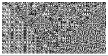
Figure 2. Spacetime diagram for a cellular automaton with generating polynomial $\phi(x)=x+1+x^{-1}\in\mathbb{F}_{2}[x]$. The dimensions are $511\times 256$. The right half $(u_{m})_{m\geq 0}$ of the initial condition is the Thue–Morse sequence, and the left half $(u_{-m})_{m\geq 0}$ is the Toeplitz sequence (the fixed point of $0\to 01,1\to 00$). By Corollary 3.15, this spacetime diagram is $[-2,2]$-automatic.

3. Algebraicity and automaticity of spacetime diagrams

In this section we show that a spacetime diagram obtained by evolving a linear cellular automaton from a $(-p)$-automatic initial condition $u$ is automatic in several senses. There is a natural notion of the $[p,p]$-kernel of a two-dimensional configuration extending the usual definition. First, if we consider bi-infinite initial conditions that satisfy $u_{m}=0$ for all $m\leq-1$, we show in Theorem 3.5 that the generating functions of these cone-indexed configurations are algebraic and that they have finite $[p,p]$-kernels. Then in Section 3.2 we show that the shear of an algebraic cone-indexed configuration is $[p,p]$-automatic. Finally, in Section 3.3 we study the $[-p,p]$-automaticity of spacetime diagrams, where the coordinates $(m,n)$ are processed by reading $m$ in base $-p$. Specifically, we prove in Corollary 3.15 that a spacetime diagram obtained by evolving a linear cellular automaton from a general $(-p)$-automatic initial condition is $[-p,p]$-automatic.

3.1. Algebraicity and finiteness of the $[p,p]$-kernel

Define the $[p,p]$-kernel of $U=(U_{m,n})_{(m,n)\in\mathbb{Z}\times\mathbb{N}}$ to be the set

$$\left\{\left(U_{p^{e}m+i,p^{e}n+j}\right)_{(m,n)\in\mathbb{Z}\times\mathbb{N}}:e\geq 0,\,0\leq i\leq p^{e}-1,\,0\leq j\leq p^{e}-1\right\}.$$

The $[p,p]$-kernel of a cone-indexed sequence $(U_{m,n})_{(m,n)\in\mathcal{C}}$ is defined by extending $U_{m,n}=0$ for all $(m,n)\in\left(\mathbb{Z}\times\mathbb{N}\right)\setminus\mathcal{C}$.

Given $i,j\in\{0,1,\dots,p-1\}$, the Cartier operator $\Lambda_{i,j}:\mathbb{F}_{p,\preceq}\llbracket x,y\rrbracket\rightarrow\mathbb{F}_{p,\preceq}\llbracket x,y\rrbracket$ is defined as

$$\Lambda_{i,j}\left(\sum_{(m,n)\in\mathcal{C}}U_{m,n}x^{m}y^{n}\right)\mathrel{\mathop{:}}=\sum_{(m,n):(mp+i,np+j)\in\mathcal{C}}U_{mp+i,np+j}x^{m}y^{n}.$$

Let $\mathcal{C}$ be a cone. The $[p,p]$-kernel of a power series $F(x,y)=\sum_{(m,n)\in\mathcal{C}}U_{m,n}x^{m}y^{n}\in\mathbb{F}_{p,\mathcal{C}}\llbracket x,y\rrbracket$ is the set

$$\left\{\Lambda_{i_{\ell},j_{\ell}}\cdots\Lambda_{i_{0},j_{0}}\left(F(x,y)\right):\text{$\ell\geq 0$ and $0\leq i_{k},j_{k}\leq p-1$ for $0\leq k\leq\ell$}\right\}.$$

If the sequence $(U_{m,n})_{(m,n)\in\mathcal{C}}$ is indexed by a cone, then its $[p,p]$-kernel is the set of all sequences $(V_{m,n})_{(m,n)\in\mathcal{C}^{*}}$ where $\sum_{(m,n)\in\mathcal{C}^{*}}V_{m,n}x^{m}y^{n}$ belongs to the $[p,p]$-kernel of $\sum_{(m,n)\in\mathcal{C}}U_{m,n}x^{m}y^{n}$. We show in Lemma 3.2 that such $\mathcal{C}^{*}$ are compatible with $\preceq$.

We can define analogously the one-dimensional Cartier operator $\Lambda_{i}:\mathbb{F}_{p}\llbracket x\rrbracket\to\mathbb{F}_{p}\llbracket x\rrbracket$ and also the $p$-kernel of a one-dimensional power series. Eilenberg’s theorem [4, Theorem 6.6.2] states that a sequence $(u_{m})_{m\geq 0}$ is $p$-automatic precisely when its $p$-kernel is finite; the same is true for a $[p,p]$-automatic sequence $(U_{m,n})_{(m,n)\in\mathbb{N}\times\mathbb{N}}$ [4, Theorem 14.4.1]. For a recent extension of Eilenberg’s theorem to automatic sequences based on some alternative numeration systems, see [26].

A power series $f(x)\in\mathbb{F}_{p}\llbracket x\rrbracket$ is algebraic over $\mathbb{F}_{p}(x)$ if there exists a nonzero polynomial $P(x,z)\in\mathbb{F}_{p}[x,z]$ such that $P(x,f(x))=0$. Similarly, the cone-indexed series $f(x,y)\in\mathbb{F}_{p,\preceq}\llbracket x,y\rrbracket$ is algebraic over $\mathbb{F}_{p}(x,y)$ if there exists a nonzero polynomial $P(x,y,z)\in\mathbb{F}_{p}[x,y,z]$ such that $P(x,y,f(x))=0$. We recall Christol’s theorem for one-dimensional power series [16, 17], generalised to two-dimensional power series by Salon [36].

Theorem 3.1.

1. A sequence $(u_{m})_{m\geq 0}$ of elements in $\mathbb{F}_{p}$ is $p$-automatic if and only if $\sum_{m\geq 0}u_{m}x^{m}$ is algebraic over $\mathbb{F}_{p}(x)$.

2. A sequence of elements $(U_{m,n})_{(m,n)\in\mathbb{N}\times\mathbb{N}}$ in $\mathbb{F}_{p}$ is $[p,p]$-automatic if and only if $\sum_{(m,n)\in\mathbb{N}\times\mathbb{N}}U_{m,n}x^{m}y^{n}$ is algebraic over $\mathbb{F}_{p}(x,y)$.

We refer to [4, Theorems 12.2.5 and 14.4.1] for the proof of Theorem 3.1, where it is shown that the algebraicity of a power series over a finite field is equivalent to the automaticity of its sequence of coefficients, which is equivalent to the finiteness of its $p$- or $[p,p]$-kernel. In related work, Allouche, Deshouillers, Kamae, and Koyanagi [3, Theorem 6] show that the coefficients of an algebraic power series in $F_{p}((x))\llbracket y\rrbracket$ is $p$-automatic.

In the next lemma we show that the image of $\mathbb{F}_{p,\preceq}\llbracket x,y\rrbracket$ under $\Lambda_{i,j}$ is indeed contained in $\mathbb{F}_{p,\preceq}\llbracket x,y\rrbracket$. We show more: although elements of the $[p,p]$-kernel of $F(x,y)\in\mathbb{F}_{p,\mathcal{C}}\llbracket x,y\rrbracket$ do not necessarily belong to $\mathbb{F}_{p,\mathcal{C}}\llbracket x,y\rrbracket$, their indexing sets are one of a finite set of translates of $\mathcal{C}$.

Lemma 3.2.

Let $r\geq 0$ be an integer, let $\mathcal{C}$ be the cone generated by $(1,0)$ and $(-r,1)$, and let $F(x,y)\in\mathbb{F}_{p,\mathcal{C}}\llbracket x,y\rrbracket$. Then every element of the $[p,p]$-kernel of $F(x,y)$ is supported on $\mathcal{C}-(t,0)$ for some $0\leq t\leq r$.

Proof.

Let $0\leq i\leq p-1$, and $0\leq j\leq p-1$. We abuse notation and define $\Lambda_{i,j}(\mathcal{C})\mathrel{\mathop{:}}=\left\{\left(\tfrac{m-i}{p},\tfrac{n-j}{p}\right):(m,n)\in\mathcal{C},\,m\equiv i\mod p,\,n\equiv j\mod p\right\}$. Let $0\leq s\leq r$. Then we claim that $\Lambda_{i,j}(\mathcal{C}-(s,0))=\mathcal{C}-(t,0)$ for some $0\leq t\leq r$. The statement of the lemma follows from the claim. Let $(m,n)\in\mathbb{Z}\times\mathbb{Z}$ be a point satisfying $n\geq 0$, $-m-rn\leq s$, $m\equiv i\mod p$, and $n\equiv j\mod p$. Then $\Lambda_{i,j}$ maps $(m,n)$ to $\left(\frac{m-i}{p},\frac{n-j}{p}\right)$, which satisfies $\frac{n-j}{p}\geq 0$ and

$$\textstyle{-\frac{m-i}{p}-r\cdot\frac{n-j}{p}\leq\frac{i+s+rj}{p}\leq\frac{(p-1)+r+r(p-1)}{p}=r+1-\frac{1}{p}}.$$

Since $-\frac{m-i}{p}-r\cdot\frac{n-j}{p}$ is an integer, this implies $-\frac{m-i}{p}-r\cdot\frac{n-j}{p}\leq t\mathrel{\mathop{:}}=\left\lfloor\frac{i+s+rj}{p}\right\rfloor$ and $t\leq r$. ∎

Example 3.3.

If $p=2$ and $\mathcal{C}$ is generated by $(1,0)$ and $(-3,1)$, then $\Lambda_{0,0}$ and $\Lambda_{1,0}$ map $\mathcal{C}$ to itself. The other Cartier operators map $\Lambda_{0,1}(\mathcal{C})=\mathcal{C}-(1,0)$ and $\Lambda_{1,1}(\mathcal{C})=\mathcal{C}-(2,0)$. The cone $\mathcal{C}-(3,0)$ arises from $\Lambda_{1,1}\Lambda_{1,1}(\mathcal{C})=\mathcal{C}-(3,0)$.

We now state Christol’s theorem for $\mathbb{F}_{p,\preceq}\llbracket x,y\rrbracket$. The case $r=0$ is Salon’s theorem (Part (2) of Theorem 3.1). We omit the proof, since it is a straightforward generalisation of the proofs in [4, Theorems 12.2.5 and 14.4.1].

Theorem 3.4.

Let $F(x,y)\in\mathbb{F}_{p,\preceq}\llbracket x,y\rrbracket$. Then $F(x,y)$ is algebraic over $\mathbb{F}_{p}(x,y)$ if and only if $F(x,y)$ has a finite $[p,p]$-kernel.

Next we prove that a linear cellular automaton begun from a $p$-automatic initial condition produces an algebraic spacetime diagram. A special case appears in Allouche et al. [6, Lemma 2], when the initial condition is eventually $0$ in both directions. The proof in the general case is similar.

Theorem 3.5.

Let $\Phi:\mathbb{F}_{p}^{\mathbb{Z}}\rightarrow\mathbb{F}_{p}^{\mathbb{Z}}$ be a linear cellular automaton. If $u\in\mathbb{F}_{p}^{\mathbb{Z}}$ is such that $(u_{m})_{m\geq 0}$ is $p$-automatic and $u_{m}=0$ for all $m\leq-1$, then the generating function of $\operatorname*{ST}_{\Phi}(u)$ is algebraic and so has a finite $[p,p]$-kernel.

Proof.

Let the generating polynomial of $\Phi$ be $\phi(x)\mathrel{\mathop{:}}=\alpha_{-\ell}x^{\ell}+\dots+\alpha_{0}+\dots+\alpha_{r}x^{-r}$. Let $f_{u}(x)\in\mathbb{F}_{p}\llbracket x\rrbracket$ be the generating function of $u$. The $n$-th row of $\operatorname*{ST}_{\Phi}(u)$ is the sequence whose generating function is the Laurent series $\phi(x)^{n}f_{u}(x)$. Let $\mathcal{C}$ be the cone generated by $(1,0)$ and $(-r,1)$. Note that $U\mathrel{\mathop{:}}=\operatorname*{ST}_{\Phi}(u)$ is identically $0$ on $\left(\mathbb{Z}\times\mathbb{N}\right)\setminus\mathcal{C}$, so its generating function satisfies $F_{U}(x,y)\in\mathbb{F}_{p,\mathcal{C}}\llbracket x,y\rrbracket\subseteq\mathbb{F}_{p,\preceq}\llbracket x,y\rrbracket$. Also,

$$F_{U}(x,y)=\sum_{n=0}^{\infty}\phi(x)^{n}f_{u}(x)y^{n}=\frac{f_{u}(x)}{1-\phi(x)y}.$$

Since $(u_{m})_{m\geq 0}$ is $p$-automatic, Part (1) of Theorem 3.1 guarantees the existence of a polynomial $P(x,z)\in\mathbb{F}_{p}[x,z]$ such that $P(x,f_{u}(x))=0$. Let $Q(x,y,z)\mathrel{\mathop{:}}=P(x,(1-\phi(x)y)z)$. Then

$$Q(x,y,F_{U}(x,y))=P(x,(1-\phi(x)y)F_{U}(x,y))=P(x,f_{u}(x))=0,$$

so $F_{U}(x,y)$ is algebraic. By Theorem 3.4, $U=(U_{m,n})_{(m,n)\in\mathcal{C}}$ has a finite $[p,p]$-kernel. ∎

In Figure 1 we have an illustration of a spacetime diagram satisfying the conditions of Theorem 3.5.

Let $\mathcal{C}$ be the cone generated by $(1,0)$ and $(-r,1)$. An interesting question is the following. Given a polynomial equation $Q(x,y,z)=0$ satisfied by $z=F(x,y)\in\mathbb{F}_{p,\mathcal{C}}\llbracket x,y\rrbracket$, is it decidable whether $F(x,y)$ is the generating function of $\operatorname*{ST}_{\Phi}(u)$ for some linear cellular automaton $\Phi$? The initial condition $u$ is determined by $F(x,0)$, so it would suffice to obtain an upper bound on the left radius $\ell$.

3.2. Automaticity by shearing

If $r\geq 1$, then the cone generated by $(1,0)$ and $(-r,1)$ contains points $(m,n)$ where $m\leq-1$. In this section, we feed these indices into an automaton by shearing the sequence so that it is supported on $\mathbb{N}\times\mathbb{N}$.

Definition 3.6.

Let $\mathcal{C}$ be the cone generated by $(1,0)$ and $(-r,1)$, and let $s\geq 0$. The shear of a sequence $(U_{m,n})_{(m,n)\in\mathcal{C}-(s,0)}$ is the sequence $(V_{m,n})_{(m,n)\in\mathbb{N}\times\mathbb{N}}$ defined by $V_{m,n}=U_{m-s-rn,n}$ for each $(m,n)\in\mathbb{N}\times\mathbb{N}$.

The next lemma enables us to move between the $[p,p]$-kernel of the generating function $\sum_{(m,n)\in\mathcal{C}}U_{m,n}x^{m}y^{n}$ of a cone-indexed sequence and the generating function $\sum_{(m,n)\in\mathbb{N}\times\mathbb{N}}V_{m,n}x^{m}y^{n}$ of its shear.

Lemma 3.7.

Let $F(x,y)\in\mathbb{F}_{p,\preceq}\llbracket x,y\rrbracket$. Let $0\leq i\leq p-1$, $0\leq j\leq p-1$. Then

$$\Lambda_{i,j}\left(x^{\ell}F(x,y)\right)=x^{-\left\lfloor\frac{i-\ell}{p}\right\rfloor}\Lambda_{(i-\ell)\bmod p,j}(F(x,y)).$$

Proof.

Let $\ell^{\prime}=-\left\lfloor\frac{i-\ell}{p}\right\rfloor$. Let $m,n\in\mathbb{Z}$. We prove the result for the monomial $F(x,y)=x^{m}y^{n}$; the general result then follows from the linearity of $\Lambda_{i,j}$. If $n\mathrel{\not\equiv}j\mod p$, then both sides are $0$. If $n\equiv j\mod p$, we have

$$\Lambda_{i,j}\left(x^{\ell}\cdot x^{m}y^{n}\right) =\Lambda_{i,j}\left(x^{\ell+m}y^{n}\right)$$

$$=\begin{cases}x^{\frac{\ell+m-i}{p}}y^{\frac{n-j}{p}}&\text{if $\ell+m\equiv i\mod p$}\\ 0&\text{otherwise}\end{cases}$$

$$=\begin{cases}x^{\ell^{\prime}+\frac{m-(i-\ell+p\ell^{\prime})}{p}}y^{\frac{n-j}{p}}&\text{if $m\equiv i-\ell+p\ell^{\prime}\mod p$}\\ 0&\text{otherwise}\end{cases}$$

$$=x^{\ell^{\prime}}\Lambda_{i-\ell+p\ell^{\prime},j}(x^{m}y^{n})$$

$$=x^{\ell^{\prime}}\Lambda_{(i-\ell)\bmod p,j}(x^{m}y^{n}).\qed$$

Note here that for each fixed $\ell$, the map $i\mapsto(i-\ell)\bmod p$ is a bijection.

Example 3.8.

Let $p=3$, and let $F(x,y)\in\mathbb{F}_{3,\preceq}\llbracket x,y\rrbracket$. For each $j$, we have

$$\Lambda_{0,j}(x^{-1}F(x,y)) =\Lambda_{1,j}(F(x,y)),$$

$$\Lambda_{1,j}(x^{-1}F(x,y)) =\Lambda_{2,j}(F(x,y)),$$

$$\Lambda_{2,j}(x^{-1}F(x,y)) =x^{-1}\Lambda_{0,j}(F(x,y)).$$

We prove a version of Eilenberg’s theorem for cone-indexed automatic sequences. We show there exists an explicit automaton representation of the shear of a cone-indexed $p$-automatic sequence using its $[p,p]$-kernel.

Theorem 3.9.

Let $\mathcal{C}$ be generated by $(1,0)$ and $(-r,1)$ for some $r\geq 0$. A $\mathcal{C}$-indexed sequence $(U_{m,n})_{(m,n)\in\mathcal{C}}$ of elements in $\mathbb{F}_{p}$ has a finite $[p,p]$-kernel if and only if its shear is $[p,p]$-automatic.

Proof.

Let $(V_{m,n})_{(m,n)\in\mathbb{N}\times\mathbb{N}}$ be the shear of $(U_{m,n})_{(m,n)\in\mathcal{C}}$. By [4, Theorem 14.2.2], $V$ is $[p,p]$-automatic if and only if its $[p,p]$-kernel is finite. Hence we show that $U$ has a finite $[p,p]$-kernel if and only if $V$ has a finite $[p,p]$-kernel.

By Lemma 3.2, every element of the $[p,p]$-kernel of $U$ is supported on $\mathcal{C}-(s,0)$ for some $0\leq s\leq r$. Let $W$ be an element of the $[p,p]$-kernel of $U$, supported on $\mathcal{C}-(s,0)$. Let $F(x,y)=\sum_{(m,n)\in\mathcal{C}-(s,0)}W_{m,n}x^{m}y^{n}$. Let $G_{n}(x,y)=x^{s+rn}\sum_{m\geq-s-rn}W_{m,n}x^{m}y^{n}$, so that $G(x,y)=\sum_{n\geq 0}G_{n}(x,y)$ is the generating function of the shear of $W$. Similarly write $F_{n}(x,y)=\sum_{m\geq-s-rn}W_{m,n}x^{m}y^{n}$; then $G_{n}(x,y)=x^{s+rn}F_{n}(x,y)$. Fix $n\equiv j\mod p$, and write $n=j+kp$ where $k\geq 0$. By Lemma 3.7, we have

$$\Lambda_{i,j}(F_{n}(x,y)) =\Lambda_{i,j}\left(x^{-s-rn}G_{n}(x,y)\right)$$

$$=x^{-\left\lfloor\frac{i+s+rn}{p}\right\rfloor}\Lambda_{(i+s+rn)\bmod p,j}(G_{n}(x,y))$$

$$=x^{-\left\lfloor\frac{i+s+rj}{p}\right\rfloor-rk}\Lambda_{(i+s+rj)\bmod p,j}(G_{j+kp}(x,y)).$$

Summing over $k\geq 0$ gives

$$\Lambda_{i,j}(F(x,y))=x^{-\left\lfloor\frac{i+s+rj}{p}\right\rfloor}\sum_{k\geq 0}x^{-rk}\Lambda_{(i+s+rj)\bmod p,j}(G_{j+kp}(x,y)).$$

Therefore the shear of $x^{\left\lfloor\frac{i+s+rj}{p}\right\rfloor}\Lambda_{i,j}(F(x,y))$ is

$$\sum_{k\geq 0}\Lambda_{(i+s+rj)\bmod p,j}(G_{j+kp}(x,y)) =\Lambda_{(i+s+rj)\bmod p,j}\left(\sum_{n\geq 0}G_{n}(x,y)\right)$$

$$=\Lambda_{(i+s+rj)\bmod p,j}\left(G(x,y)\right).$$

Inductively, suppose $G(x,y)$ is the generating function of an element of the kernel of $V$. Then the shear of $x^{\left\lfloor\frac{i+s+rj}{p}\right\rfloor}\Lambda_{i,j}(F(x,y))$ is an element of the $[p,p]$-kernel of $V$. Note that $\Lambda_{i,j}(F(x,y))$ is supported on $\mathcal{C}-\left(\left\lfloor\frac{i+s+rj}{p}\right\rfloor,0\right)$.

We set up a map $\kappa$ from the $[p,p]$-kernel of $U$ to the $[p,p]$-kernel of $V$. Let $\kappa(U)=V$, and define $\kappa$ recursively as follows. For each $W$ in the $[p,p]$-kernel of $U$, let $\kappa(\Lambda_{i,j}(W))=\Lambda_{(i+s+rj)\bmod p,j}(\kappa(W))$ where $W$ is supported on $\mathcal{C}-(s,0)$. Since the map $i\mapsto(i+s+rj)\bmod p$ is a bijection on $\mathbb{F}_{p}$, $\kappa$ maps $\{\Lambda_{i,j}(W):0\leq i,j\leq p-1\}$ surjectively onto $\{\Lambda_{i,j}(\kappa(W)):0\leq i,j\leq p-1\}$. It follows inductively that $\kappa$ is a surjection from the $[p,p]$-kernel of $U$ to the $[p,p]$-kernel of $V$.

If the $[p,p]$-kernel of $U$ is finite, then the surjectivity of $\kappa$ implies that the $[p,p]$-kernel of $V$ is finite. By Lemma 3.2, $\kappa$ is at most $(r+1)$-to-one. Therefore if the $[p,p]$-kernel of $V$ is finite then the $[p,p]$-kernel of $U$ has at most $r+1$ times as many elements and is also finite. ∎

We can now extend Theorem 3.5.

Theorem 3.10.

Let $\Phi:\mathbb{F}_{p}^{\mathbb{Z}}\rightarrow\mathbb{F}_{p}^{\mathbb{Z}}$ be a linear cellular automaton. If $u\in\mathbb{F}_{p}^{\mathbb{Z}}$ is such that $(u_{m})_{m\geq 0}$ is $p$-automatic and $u_{m}=0$ for all $m\leq-1$, then the shear of $\operatorname*{ST}_{\Phi}(u)$ is $[p,p]$-automatic.

Proof.

By Theorem 3.5, $\operatorname*{ST}_{\Phi}(u)$ has a finite $[p,p]$-kernel. By Theorem 3.9, we conclude that the shear of $\operatorname*{ST}_{\Phi}(u)$ is $[p,p]$-automatic. ∎

      

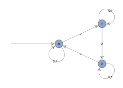
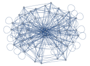
Figure 3. Automata from Example 3.11. The automaton on the left generates the initial condition $u$, and the automaton on the right generates the spacetime diagram $\operatorname*{ST}_{\Phi}(u)$.

Example 3.11.

Let $p=3$, and let $\phi(x)=x+1\in\mathbb{F}_{3}[x]$. Let $(u_{m})_{m\geq 0}$ be the $3$-automatic sequence generated by the automaton on the left in Figure 3, whose first few terms are $001001112\cdots$. The size of this automaton makes later computations feasible. Let $u_{m}=0$ for all $m\leq-1$; then the spacetime diagram $U=\operatorname*{ST}_{\Phi}(u)$ is supported on $\mathbb{N}\times\mathbb{N}$. See Figure 4. We compute an automaton for the $[3,3]$-automatic sequence $U|_{\mathbb{N}\times\mathbb{N}}$. By Part (1) of Theorem 3.1, we can compute a polynomial $P(x,y)$ such that $P(x,f_{u}(x))=0$. We compute

$$P(x,y)=x^{28}y+2\left(x^{12}+x^{21}+x^{24}+x^{27}+x^{28}+x^{29}\right)y^{3}\\ +\left(1+2x^{9}+x^{12}+x^{15}+x^{18}+x^{21}+2x^{24}+2x^{27}+x^{30}\right)y^{9}\\ +2\left(1+x^{27}+x^{54}\right)y^{27}.$$

Note that this is not the minimal polynomial for $f_{u}(x)$, but it is in a convenient form for the subsequent computation. As in the proof of Theorem 3.5, the generating function $F_{U}(x,y)$ of $U$ satisfies $P(x,(1-\phi(x)y)F_{U}(x,y))=0$. By Part (2) of Theorem 3.1, we can use this polynomial equation to compute an automaton for $U|_{\mathbb{N}\times\mathbb{N}}$. The resulting automaton has $486$ states; minimizing produces an equivalent automaton with $54$ states. This automaton is shown without labels or edge directions on the right in Figure 3. These computations were performed with the Mathematica package IntegerSequences [34].

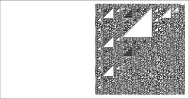
Figure 4. Spacetime diagram for a cellular automaton with generating polynomial $\phi(x)=x+1\in\mathbb{F}_{3}[x]$. The initial condition is generated by the automaton in Example 3.11. The line $n=m$ separates the diagram into two regions; the upper region contains arbitrarily large white patches, and the lower region does not. This is because the left half of the initial condition is identically $0$. The dimensions are $511\times 256$.

3.3. Automaticity in base $[-p,p]$

Instead of shearing, we may evaluate an automaton at negative integers by using base $-p$. This approach gives a variant of Theorem 3.9 and a notion of automaticity of $\operatorname*{ST}_{\Phi}(u)$ for a general $(-p)$-automatic initial condition $u$.

Definition 3.12.

A sequence $(U_{m,n})_{(m,n)\in\mathbb{Z}\times\mathbb{N}}$ is $[-p,p]$-automatic if there is a DFAO $(\mathcal{S},\{0,\dots,p-1\}^{2},\delta,s_{0},\mathbb{F}_{p},\omega)$ such that

$$U_{m,n}=\omega(\delta(s_{0},(m_{\ell},n_{\ell})\cdots(m_{1},n_{1})(m_{0},n_{0})))$$

for all $(m,n)\in\mathbb{N}\times\mathbb{N}$, where $m_{\ell}\cdots m_{1}m_{0}$ is the standard base-$(-p)$ representation of $m$ and $n_{\ell}\cdots n_{1}n_{0}$ is the standard base-$p$ representation of $n$, padded with zeros if necessary, as in Section 2.3.

Theorem 3.13.

A sequence $(U_{m,n})_{(m,n)\in\mathbb{Z}\times\mathbb{N}}$ has a finite $[p,p]$-kernel if and only if it is $[-p,p]$-automatic.

Proof.

Define the $[-p,p]$-Cartier operator $\bar{\Lambda}_{i,j}$ by

$$\bar{\Lambda}_{i,j}\left((W_{m,n})_{(m,n)\in\mathbb{Z}\times\mathbb{N}}\right)\mathrel{\mathop{:}}=(W_{-pm+i,pn+j})_{(m,n)\in\mathbb{Z}\times\mathbb{N}}.$$

Define the $[-p,p]$-kernel of $U=(U_{m,n})_{(m,n)\in\mathbb{Z}\times\mathbb{N}}$ to be the smallest set containing $U$ that is closed under $\bar{\Lambda}_{i,j}$ for all $i,j\in\{0,1,\dots,p-1\}$. We show that the $[p,p]$-kernel of $U$ is finite if and only if the $[-p,p]$-kernel of $U$ is finite.

For a sequence $(W_{m,n})_{(m,n)\in\mathbb{Z}\times\mathbb{N}}$, define $\rho(W)\mathrel{\mathop{:}}=(W_{-m,n})_{(m,n)\in\mathbb{Z}\times\mathbb{N}}$ and $\sigma^{-1}(W)\mathrel{\mathop{:}}=(W_{m-1,n})_{(m,n)\in\mathbb{Z}\times\mathbb{N}}$. Let $K$ be the union, over all elements $W$ in the $[p,p]$-kernel of $U$, of the set

$$\left\{W,\,\rho(W),\,\sigma^{-1}(W),\,\rho(\sigma^{-1}(W))\right\}.$$

We claim that the $[-p,p]$-kernel of $U$ is a subset of $K$. One verifies that $\bar{\Lambda}_{i,j}(K)\subseteq K$:

$$\bar{\Lambda}_{i,j}(W) =\rho(\Lambda_{i,j}(W))$$

$$\bar{\Lambda}_{i,j}(\rho(W)) =\begin{cases}\Lambda_{0,j}(W)&\text{if $i=0$}\\ \sigma^{-1}(\Lambda_{p-i,j}(W))&\text{if $i\neq 0$}\end{cases}$$

$$\bar{\Lambda}_{i,j}(\sigma^{-1}(W)) =\begin{cases}\rho(\sigma^{-1}(\Lambda_{p-1,j}(W)))&\text{if $i=0$}\\ \rho(\Lambda_{i-1,j}(W))&\text{if $i\neq 0$}\end{cases}$$

$$\bar{\Lambda}_{i,j}(\rho(\sigma^{-1}(W))) =\sigma^{-1}(\Lambda_{p-1-i,j}(W)).$$

For example, if $i\neq 0$ we have

$$\bar{\Lambda}_{i,j}(\rho(W)) =\bar{\Lambda}_{i,j}\left((W_{-m,n})_{(m,n)\in\mathbb{Z}\times\mathbb{N}}\right)$$

$$=(W_{-(-pm+i),pn+j})_{(m,n)\in\mathbb{Z}\times\mathbb{N}}$$

$$=(W_{p(m-1)+p-i,pn+j})_{(m,n)\in\mathbb{Z}\times\mathbb{N}}$$

$$=\sigma^{-1}\left((W_{pm+p-i,pn+j})_{(m,n)\in\mathbb{Z}\times\mathbb{N}}\right)$$

$$=\sigma^{-1}(\Lambda_{p-i,j}(W));$$

the other identities follow similarly. Since $U\in K$, it follows that the $[-p,p]$-kernel of $U$ is a subset of $K$. Therefore there are at most four times as many elements in the $[-p,p]$-kernel as in the $[p,p]$-kernel, so if the $[p,p]$-kernel is finite then the $[-p,p]$-kernel is also finite.

Similarly, we can emulate $\Lambda_{i,j}$ by taking the four states $W,\rho(W),\sigma(W),\sigma(\rho(W))$ for each element $W$ in the $[-p,p]$-kernel of $U$, where $\sigma(W)\mathrel{\mathop{:}}=(W_{m+1,n})_{(m,n)\in\mathbb{Z}\times\mathbb{N}}$:

$$\Lambda_{i,j}(W) =\rho(\bar{\Lambda}_{i,j}(W))$$

$$\Lambda_{i,j}(\rho(W)) =\begin{cases}\bar{\Lambda}_{0,j}(W)&\text{if $i=0$}\\ \sigma(\bar{\Lambda}_{p-i,j}(W))&\text{if $i\neq 0$}\end{cases}$$

$$\Lambda_{i,j}(\sigma(W)) =\begin{cases}\sigma(\rho(\bar{\Lambda}_{0,j}(W)))&\text{if $i=p-1$}\\ \rho(\bar{\Lambda}_{i+1,j}(W))&\text{if $i\neq p-1$}\end{cases}$$

$$\Lambda_{i,j}(\sigma(\rho(W))) =\sigma(\bar{\Lambda}_{p-1-i,j}(W)).$$

It follows that there are at most four times as many elements in the $[p,p]$-kernel as in the $[-p,p]$-kernel, so if the $[-p,p]$-kernel is finite then the $[p,p]$-kernel is also finite.

Now we show that the $[-p,p]$-kernel of $U$ is finite if and only if $U$ is $[-p,p]$-automatic. The proof is similar to the usual proof of Eilenberg’s characterisation, as in [4, Theorem 6.6.2]. If the $[-p,p]$-kernel of $U$ is finite, then the automaton whose states are the elements of the $[-p,p]$-kernel and whose transitions are determined by the action of $\bar{\Lambda}_{i,j}$ is finite; moreover, this automaton outputs $U_{m,n}$ when fed the base-$[-p,p]$ representation of $(m,n)$. Conversely, if there is such an automaton, then the $[-p,p]$-kernel is finite since it can be embedded into the set of states of the automaton. ∎

Theorem 3.14.

Let $\Phi:\mathbb{F}_{p}^{\mathbb{Z}}\rightarrow\mathbb{F}_{p}^{\mathbb{Z}}$ be a linear cellular automaton. If $u\in\mathbb{F}_{p}^{\mathbb{Z}}$ is such that $(u_{m})_{m\geq 0}$ is $p$-automatic and $u_{m}=0$ for all $m\leq-1$, then $\operatorname*{ST}_{\Phi}(u)$ is $[-p,p]$-automatic.

Proof.

By Theorem 3.5, $\operatorname*{ST}_{\Phi}(u)$ has a finite $[p,p]$-kernel. By Theorem 3.13, $\operatorname*{ST}_{\Phi}(u)$ is $[-p,p]$-automatic. ∎

Corollary 3.15.

Let $\Phi:\mathbb{F}_{p}^{\mathbb{Z}}\rightarrow\mathbb{F}_{p}^{\mathbb{Z}}$ be a linear cellular automaton. If $u\in\mathbb{F}_{p}^{\mathbb{Z}}$ is $(-p)$-automatic, then $\operatorname*{ST}_{\Phi}(u)$ is $[-p,p]$-automatic.

Proof.

Consider the two initial conditions $\cdots u_{-2}u_{-1}\cdot 00\cdots$ and $\cdots 00\cdot u_{0}u_{1}\cdots$. By Theorem 3.14, $\operatorname*{ST}_{\Phi}(\cdots 00\cdot u_{0}u_{1}\cdots)$ is $[-p,p]$-automatic. A straightforward modification of Theorem 3.14 shows that $\operatorname*{ST}_{\Phi}(\cdots u_{-2}u_{-1}\cdot 00\cdots)$ is also $[-p,p]$-automatic. Since $\Phi$ is linear, $\operatorname*{ST}_{\Phi}(u)$ is the termwise sum of these two spacetime diagrams. The sum of two $[-p,p]$-automatic sequences is automatic; therefore $\operatorname*{ST}_{\Phi}(u)$ is $[-p,p]$-automatic. ∎

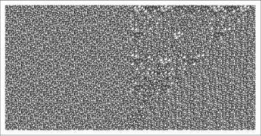
Figure 5. Spacetime diagram for the linear cellular automaton with generating polynomial $\phi(x)=x+1\in\mathbb{F}_{3}[x]$ begun from the $3$-automatic initial condition described in Example 3.16. The dimensions are $511\times 256$.

Example 3.16.

As in Example 3.11, let $p=3$, let $\phi(x)=x+1\in\mathbb{F}_{3}[x]$, and let $(u_{m})_{m\geq 0}$ be $3$-automatic sequence generated by the automaton on the left in Figure 3. We extend $(u_{m})_{m\geq 0}$ to a $(-3)$-automatic sequence $(u_{m})_{m\in\mathbb{Z}}$ by setting $u_{m}=u_{-m}$ for all $m\leq-1$. The resulting spacetime diagram is shown in Figure 5. By Corollary 3.15, $\operatorname*{ST}_{\Phi}(u)$ is $[-3,3]$-automatic.

To compute an automaton for $\operatorname*{ST}_{\Phi}(u)$, we start with the $54$-state automaton computed in Example 3.11 for the right half $(U_{m,n})_{(m,n)\in\mathbb{N}\times\mathbb{N}}$ of the spacetime diagram in Figure 4. We convert this $[3,3]$-automaton using Theorem 3.13 to a $[-3,3]$-automaton for the spacetime diagram $(U_{m,n})_{(m,n)\in\mathbb{Z}\times\mathbb{N}}$ in Figure 4 whose left half is identically $0$; minimizing produces an automaton $\mathcal{M}$ with $204$ states.

We also need an automaton for the $\mathbb{Z}\times\mathbb{N}$-indexed spacetime diagram with initial condition $\cdots u_{-2}u_{-1}000\cdots$, shown in Figure 6. The symmetry $x^{-1}\phi(x)=\phi(x^{-1})$ implies that a shear of this diagram is the left–right reflection $(U_{-m,n})_{(m,n)\in\mathbb{Z}\times\mathbb{N}}$ of the diagram in Figure 4. Since $(U_{-m,n})_{(m,n)\in\mathbb{Z}\times\mathbb{N}}$ is an element of the $[-3,3]$-kernel of $U$, we obtain an automaton for $(U_{-m,n})_{(m,n)\in\mathbb{Z}\times\mathbb{N}}$ simply by changing the initial state in $\mathcal{M}$ to be the state corresponding to this kernel sequence; hence $(U_{-m,n})_{(m,n)\in\mathbb{Z}\times\mathbb{N}}$ is generated by an automaton $\mathcal{M}^{\prime}$ with $204$ states. Shearing $(U_{-m,n})_{(m,n)\in\mathbb{Z}\times\mathbb{N}}$ produces $(U_{-m+n,n})_{(m,n)\in\mathbb{Z}\times\mathbb{N}}$, the spacetime diagram in Figure 6. Using a variant of Theorem 3.9 for the $[-p,p]$-kernel of a $\mathbb{Z}\times\mathbb{N}$-indexed sequence, we compute an automaton with $204$ states for this spacetime diagram.

Finally, since $u_{0}=0$, the product of the automata for $(U_{m,n})_{(m,n)\in\mathbb{Z}\times\mathbb{N}}$ and $(U_{-m+n,n})_{(m,n)\in\mathbb{Z}\times\mathbb{N}}$ is an automaton for the sum $\operatorname*{ST}_{\Phi}(u)$ of the spacetime diagrams in Figures 4 and 6, which is the diagram in Figure 5. The product automaton has $204^{2}$ states, but minimizing reduces this to $1908$ states.

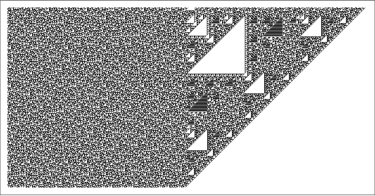
Figure 6. Spacetime diagram whose sum with the diagram in Figure 4 is the diagram in Figure 5.

4. Automaticity of $\mathbb{Z}\times\mathbb{Z}$-indexed spacetime diagrams

In Corollary 3.15, we showed that if $u$ is $(-p)$-automatic then the $\mathbb{Z}\times\mathbb{N}$-configuration $\operatorname*{ST}_{\Phi}(u)$ is $[-p,p]$-automatic. Our aim in this section is to extend Corollary 3.15 to $\mathbb{Z}\times\mathbb{Z}$-configurations. We remark that the results of this section can be further extended to statements about two-dimensional linear recurrences with constant coefficients. We also note that Bousquet-Mélou and Petkov̌sek [13] prove similar results, with different proofs, for linear recurrences on $\mathbb{N}\times\mathbb{N}$ over fields of characteristic $0$.

Definition 4.1.

If $U\in\mathbb{F}_{p}^{\mathbb{Z}\times\mathbb{Z}}$ satisfies $\Phi(U|_{\mathbb{Z}\times\{n\}})=U|_{\mathbb{Z}\times\{n+1\}}$ for each $n\in\mathbb{Z}$, we call $U$ a spacetime diagram for $\Phi$.

Note that if $\Phi:\mathbb{F}_{p}^{\mathbb{Z}}\rightarrow\mathbb{F}_{p}^{\mathbb{Z}}$ is a linear cellular automaton with left and right radii $\ell$ and $r$ respectively, then it is surjective, and every sequence in $\mathbb{F}_{p}^{\mathbb{Z}}$ has $p^{\ell+r}$ preimages. Hence if $\ell+r\geq 1$ there are infinitely many $\mathbb{Z}\times\mathbb{Z}$-indexed spacetime diagrams $U$ such that $U|_{\mathbb{Z}\times\{0\}}=u$.

Let $\Phi$ have generating polynomial $\phi(x)=\alpha_{-\ell}x^{\ell}+\dots+\alpha_{0}+\dots+\alpha_{r}x^{-r}$. A configuration $U=(U_{m,n})_{(m,n)\in\mathbb{Z}\times\mathbb{Z}}$ is a spacetime diagram for $\Phi$ if and only if

$$(1-\phi(x)y)\sum_{(m,n)\in\mathbb{Z}\times\mathbb{Z}}U_{m,n}x^{m}y^{n}=0.$$

In the following lemma we identify which initial conditions determine a spacetime diagram for $\Phi$.

Lemma 4.2.

Let $\Phi:\mathbb{F}_{p}^{\mathbb{Z}}\rightarrow\mathbb{F}_{p}^{\mathbb{Z}}$ be a linear cellular automaton with generating polynomial $\phi(x)=\alpha_{-\ell}x^{\ell}+\dots+\alpha_{0}+\dots+\alpha_{r}x^{-r}$. Let

$$\mathbb{I}=(\mathbb{Z}\times\{0\})\cup\bigcup_{i=0}^{\ell+r-1}(\{i\}\times-\mathbb{N}).$$

Then every $U\in\mathbb{F}_{p}^{\mathbb{I}}$ can be uniquely extended to a spacetime diagram $U\in\mathbb{F}_{p}^{\mathbb{Z}\times\mathbb{Z}}$ for $\Phi$.

Proof.

Note that $U|_{\mathbb{Z}\times\{0\}}$ uniquely determines a $\mathbb{Z}\times\mathbb{N}$-indexed spacetime diagram for $\Phi$. Next we observe that $U|_{(\mathbb{Z}\times\{0\})\cup\{(0,-1),\dots,(\ell+r-1,-1)\}}$ determines $U|_{\mathbb{Z}\times\{-1\}}$ for $\Phi$. For, given a word $w\in\mathbb{F}_{p}^{\ell+r}$, there is a unique sequence $v\in\mathbb{F}_{p}^{\mathbb{Z}}$ such that $v_{0}\cdots v_{\ell+r-1}=w$ and $\Phi(v)=U|_{\mathbb{Z}\times\{0\}}$. Similarly, $U|_{(\mathbb{Z}\times\{-n\})\cup\{(0,-n-1),\dots,(\ell+r-1,-n-1)\}}$ determines $U|_{\mathbb{Z}\times\{-n-1\}}$. We can repeat this, determining one row at a time, once we have specified a word of length $\ell+r$ in that row. ∎

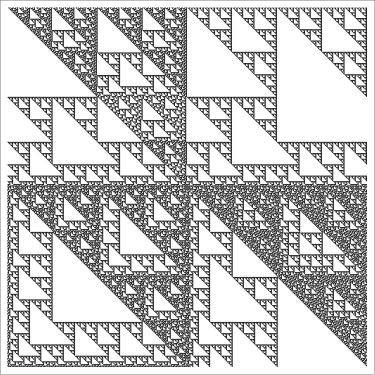
Figure 7. A $\mathbb{Z}\times\mathbb{Z}$-indexed spacetime diagram for the Ledrappier cellular automaton. The initial conditions are $U_{m,0}=T(m)$ for $m\geq 0$, $U_{m,0}=T(-m)$ for $m\leq-1$, and $U_{0,n}=T(-n)$ for $n\leq-1$, where $T(m)_{m\geq 0}$ is the Thue–Morse sequence. The dimensions are $511\times 511$.

Example 4.3.

Consider the Ledrappier cellular automaton $\Phi$, whose generating polynomial is $\phi(x)=1+x^{-1}$. By Lemma 4.2, $U$ is determined by its values on $(\mathbb{Z}\times\{0\})\cup(\{0\}\times-\mathbb{N})$. See Figure 7 for an example of a spacetime diagram for $\Phi$.

Definition 3.12 naturally generalises to $[p,q]$-automaticity for any integers $p,q$ with $|p|\geq 2$ and $|q|\geq 2$. Therefore we may consider $[-p,-p]$-automaticity. One can also define $[p,p]$-automaticity for any of the four quadrants $(\pm\mathbb{N})\times(\pm\mathbb{N})$.

Proposition 4.4.

A sequence $U\in\mathbb{F}_{p}^{\mathbb{Z}\times\mathbb{Z}}$ is $[-p,-p]$-automatic if and only if each of $U|_{(\pm\mathbb{N})\times(\pm\mathbb{N})}$ is $[p,p]$-automatic.

The proof of Proposition 4.4 follows the same lines as that of [4, Theorem 5.3.2].

Theorem 4.5.

Let $\Phi:\mathbb{F}_{p}^{\mathbb{Z}}\rightarrow\mathbb{F}_{p}^{\mathbb{Z}}$ be a linear cellular automaton with left and right radii $\ell$ and $r$. Let $U\in\mathbb{F}_{p}^{\mathbb{Z}\times\mathbb{Z}}$ be a spacetime diagram for $\Phi$. If $U|_{\{i\}\times-\mathbb{N}}$ is $p$-automatic for each $i$ in the interval $-\ell\leq i\leq r-1$ and $U|_{\mathbb{Z}\times\{0\}}$ is $(-p)$-automatic, then $U$ is $[-p,-p]$-automatic.

Proof.

By Lemma 4.2, $U$ is uniquely determined by its values on $(\mathbb{Z}\times\{0\})\cup\bigcup_{i=-\ell}^{r}(\{i\}\times-\mathbb{N})$. By Proposition 4.4 it is sufficient to show that each of the four quadrants $U|_{(\pm\mathbb{N})\times(\pm\mathbb{N})}$ is $[p,p]$-automatic.

By Corollary 3.15, $U|_{\mathbb{Z}\times\mathbb{N}}$ is $[-p,p]$-automatic. By Theorem 3.13, $U|_{\mathbb{Z}\times\mathbb{N}}$ has a finite $[p,p]$-kernel. Thus each of $U|_{\pm\mathbb{N}\times\mathbb{N}}$ has a finite $[p,p]$-kernel. By Theorem 3.9 with $r=0$, each of $U|_{\pm\mathbb{N}\times\mathbb{N}}$ is $[p,p]$-automatic.

We show that $U|_{\mathbb{N}\times-\mathbb{N}}$ is $[p,p]$-automatic; the automaticity of $U|_{-\mathbb{N}\times-\mathbb{N}}$ follows by a similar argument. Let $\phi(x)=\alpha_{-\ell}x^{\ell}+\dots+\alpha_{0}+\dots+\alpha_{r}x^{-r}$ be the generating polynomial of $\Phi$. For $S\subseteq\mathbb{Z}\times\mathbb{Z}$, let $F|_{S}$ denote the generating function of $U|_{S}$. Since $U$ is a spacetime diagram for $\Phi$, we have $U_{m,n+1}-\sum_{i=-\ell}^{r}\alpha_{i}U_{m+i,n}=0$ for each $(m,n)\in\mathbb{Z}\times\mathbb{Z}$. Multiplying by $x^{m}y^{n+1}$ and summing over $m\geq 0$ and $n\leq-1$ gives

$$0 =\sum_{\begin{subarray}{c}m\geq 0\\ n\leq-1\end{subarray}}U_{m,n+1}x^{m}y^{n+1}-\sum_{\begin{subarray}{c}m\geq 0\\ n\leq-1\end{subarray}}\sum_{i=-\ell}^{r}\alpha_{i}U_{m+i,n}x^{m}y^{n+1}$$

$$=F|_{\mathbb{N}\times-\mathbb{N}}-\sum_{i=-\ell}^{r}\alpha_{i}x^{-i}y\left(\sum_{\begin{subarray}{c}m\geq 0\\ n\leq-1\end{subarray}}U_{m+i,n}x^{m+i}y^{n}\right)$$

$$=F|_{\mathbb{N}\times-\mathbb{N}}-\sum_{i=-\ell}^{-1}\alpha_{i}x^{-i}y\left(\sum_{k=-\ell}^{i}F|_{\{k\}\times-\mathbb{N}}+F|_{\mathbb{N}\times-\mathbb{N}}-F|_{\mathbb{N}\times\{0\}}-P_{i}(x)\right)$$

$$\phantom{00}-\alpha_{0}y\left(F|_{\mathbb{N}\times-\mathbb{N}}-F|_{\mathbb{N}\times\{0\}}\right)-\sum_{i=1}^{r-1}\alpha_{i}x^{-i}y\left(F|_{\mathbb{N}\times-\mathbb{N}}-\sum_{k=0}^{i-1}F|_{\{k\}\times-\mathbb{N}}-F|_{\mathbb{N}\times\{0\}}+P_{i}(x)\right)$$

$$=(1-\phi(x)y)F|_{\mathbb{N}\times-\mathbb{N}}+\phi(x)yF|_{\mathbb{N}\times\{0\}}$$

$$\phantom{00}-\sum_{i=-\ell}^{-1}\alpha_{i}x^{-i}y\left(\sum_{k=-\ell}^{i}F|_{\{k\}\times-\mathbb{N}}\right)+\sum_{i=1}^{r-1}\alpha_{i}x^{-i}y\left(\sum_{k=0}^{i-1}F|_{\{k\}\times-\mathbb{N}}+P_{i}(x)\right),$$

where $P_{i}(x)$ are Laurent polynomials to account for over- and under-counting. Since each $U|_{\{k\}\times-\mathbb{N}}$ and $U|_{\mathbb{N}\times\{0\}}$ is automatic, each $F|_{\{k\}\times-\mathbb{N}}$ and $F|_{\mathbb{N}\times\{0\}}$ are algebraic by Part (1) of Theorem 3.1. Hence

$$F|_{\mathbb{N}\times-\mathbb{N}}=\frac{G(x,y)}{1-\phi(x)y}$$

where $G(x,y)$ is algebraic. Therefore $F|_{\mathbb{N}\times-\mathbb{N}}$ is algebraic, and $U|_{\mathbb{N}\times-\mathbb{N}}$ is $[p,p]$-automatic by Part (2) of Theorem 3.1. ∎

Example 4.6.

Consider the Ledrappier cellular automaton with $\phi(x)=1+x^{-1}$, and let

$$L_{1} =\mathbb{N}\times\{0\}$$

$$L_{2} =\{0\}\times-\mathbb{N}$$

so that $U|_{L_{1}\cup L_{2}}$ determines $U|_{\mathbb{N}\times-\mathbb{N}}$ for $\Phi$.

We have $U_{m,n}+U_{m+1,n}-U_{m,n+1}=0$ for each $(m,n)\in\mathbb{Z}\times\mathbb{Z}$, so, following the proof and notation of Theorem 4.5, we have

$$0=F|_{\mathbb{N}\times-\mathbb{N}}-y\left(F|_{\mathbb{N}\times-\mathbb{N}}-F|_{L_{1}}\right)-x^{-1}y\left(F|_{\mathbb{N}\times-\mathbb{N}}-F|_{L_{1}}-F|_{L_{2}}+U_{0,0}\right)$$

and therefore

$$F|_{\mathbb{N}\times-\mathbb{N}}=\frac{x^{-1}yU_{0,0}-(1+x^{-1})yF|_{L_{1}}-x^{-1}yF|_{L_{2}}}{1-(1+x^{-1})y}.$$

If $F|_{L_{1}}$ and $F|_{L_{2}}$ are both algebraic, then $F|_{\mathbb{N}\times-\mathbb{N}}$ is also.

As we converted the $[p,p]$-kernel to the $[-p,p]$-kernel in Theorem 3.13, one can also convert the $[-p,p]$-kernel of a spacetime diagram in Theorem 4.5 to the $[-p,-p]$-kernel. For example, this enables one to compute a $[-p,-p]$-automaton for the spacetime diagram in Figure 7.

5. Invariant sets for linear cellular automata

In this section and the next we apply the automaticity of spacetime diagrams, as shown in Corollary 3.15 and Theorem 4.5, to two related questions in symbolic dynamics. We consider the $\mathbb{Z}\times\mathbb{Z}$-dynamical system $(\mathbb{F}_{p}^{\mathbb{Z}},\sigma,\Phi)$ generated by the left shift map $\sigma$ and a linear cellular automaton $\Phi$, and we find closed subsets of $\mathbb{F}_{p}^{\mathbb{Z}}$ which are invariant under both $\sigma$ and $\Phi$. In Section 6 we find nontrivial measures $\mu$ on $\mathbb{F}_{p}^{\mathbb{Z}}$ that are invariant under the action of $\sigma$ and $\Phi$.

By a simple transfer principle, these questions can be approached by considering dynamical systems generated by spacetime diagrams $U$ for $\Phi$. Given a spacetime diagram $U$, one considers the subshift $(X_{U},\sigma_{1},\sigma_{2})$, a $\mathbb{Z}\times\mathbb{Z}$-dynamical system generated by $U$; this is defined in Section 5.1. If $U$ is automatic, then $X_{U}$ is small in the sense of Theorem 5.2.

The maps $\sigma$ and $\Phi$ do not exhibit the topological rigidity that Furstenberg’s setting yields, as mentioned in the Introduction. An example of a $(\sigma,\Phi)$-invariant set was first pointed out by Kitchens and Schmidt [25, Construction 5.2] and elaborated by Einsiedler [21]. In Theorem 5.8 we identify a large family of $(\sigma,\Phi)$-invariant sets, and we discuss the relationship between our invariant sets and those that are obtained by the method in [25].

5.1. Subshifts generated by $[-p,-p]$-automatic spacetime diagrams

In this section we set up the necessary background, define subshifts generated by a spacetime diagram, and show that the subshift generated by an automatic spacetime diagram is small but infinite. We also define substitutions, linking them to automaticity.

We equip $\mathbb{F}_{p}$ with the discrete topology and the sets $\mathbb{F}_{p}^{\mathbb{Z}}$ and $\mathbb{F}_{p}^{\mathbb{Z}\times\mathbb{Z}}$ with the metrisable product topology, noting that with this topology they are compact. Let $\sigma_{1}:\mathbb{F}_{p}^{\mathbb{Z}\times\mathbb{Z}}\rightarrow\mathbb{F}_{p}^{\mathbb{Z}\times\mathbb{Z}}$ denote the left shift map $(U_{m,n})_{(m,n)\in\mathbb{Z}\times\mathbb{Z}}\mapsto(U_{m+1,n})_{(m,n)\in\mathbb{Z}\times\mathbb{Z}}$, and let $\sigma_{2}:\mathbb{F}_{p}^{\mathbb{Z}\times\mathbb{Z}}\rightarrow\mathbb{F}_{p}^{\mathbb{Z}\times\mathbb{Z}}$ denote the down shift map $(U_{m,n})_{(m,n)\in\mathbb{Z}\times\mathbb{Z}}\mapsto(U_{m,n+1})_{(m,n)\in\mathbb{Z}\times\mathbb{Z}}$. With the notation of Section 2.1, applying the left shift (down shift) to a sequence is equivalent to multiplying its generating function by $x^{-1}$ ($y^{-1}$).

Definition 5.1.

Let $S$ and $T$ be transformations on $X$. A set $Z\subset X$ is $T$-invariant if $T(Z)\subset Z$, and $Z$ is $(S,T)$-invariant if it is both $S$- and $T$-invariant. A (two-dimensional) subshift $(X,\sigma_{1},\sigma_{2})$ is a dynamical system with $X$ a closed, $\sigma_{1}$- and $\sigma_{2}$-invariant subset of $\mathbb{F}_{p}^{\mathbb{Z}\times\mathbb{Z}}$.

We can similarly define a one-dimensional subshift $(X,\sigma)$: here $X$ is a closed, $\sigma$-invariant subset of $\mathbb{F}_{p}^{\mathbb{Z}}$ and $\sigma$ is the left shift map. We call $X$ the shift space.

Let $S\subseteq\mathbb{Z}\times\mathbb{Z}$ be a rectangle $[m_{1},m_{2}]\times[n_{1},n_{2}]$. A word on $S$ is a map $w:S\to\mathbb{F}_{p}$. These words are higher-dimensional analogues of words in one dimension, i.e. those indexed by a finite interval in $\mathbb{Z}$. If $U\in\mathbb{F}_{p}^{\mathbb{Z}\times\mathbb{Z}}$, then $U|_{S}$ is the word $(U_{m,n})_{(m,n)\in S}$, and we say that the word $U|_{S}$ occurs in $U$. Given a configuration $U\in\mathbb{F}_{p}^{\mathbb{Z}\times\mathbb{Z}}$, the language $\mathcal{L}_{U}$ of $U$ is the set of all words that occur in $U$. The language $\mathcal{L}_{X}$ of a shift space $X$ is the set of all words that occur in some configuration $U\in X$. A subword of the word $w:S\to\mathbb{F}_{p}$ is a restriction of $w$ to some rectangular $S^{\prime}\subseteq S$. The language $\mathcal{L}_{X}$ is closed under the taking of subwords, and every word in the language is extendable to a configuration in $X$. Conversely, a language $\mathcal{L}$ on $\mathbb{F}_{p}$ which is closed under the taking of subwords defines a (possibly empty) subshift $(X_{\mathcal{L}},\sigma_{1},\sigma_{2})$, where $X_{\mathcal{L}}$ is the set of configurations all of whose subwords belong to $\mathcal{L}$.

Note that we can also define the language of an $\mathbb{N}\times\mathbb{N}$- or $\mathbb{Z}\times\mathbb{N}$-configuration $U$ and, in an analogous manner, of the $\mathbb{Z}\times\mathbb{Z}$-subshift $(X_{U},\sigma_{1},\sigma_{2})$.

Let $U$ be a two-dimensional configuration. Recall the complexity function $c_{U}:\mathbb{N}\times\mathbb{N}\rightarrow\mathbb{N}$, where $c_{U}(m,n)$ is the number of distinct $m\times n$ words that occur in $U$. We remark that the second statement of the following theorem can be improved but is sufficient for our purposes.

Theorem 5.2.

1. If the sequence $U\in\mathbb{F}_{p}^{\mathbb{N}\times\mathbb{N}}$ is $[p,p]$-automatic, then for some $K$, its complexity function satisfies $c_{U}(m,n)\leq K\max\{m,n\}^{2}$.

2. If the sequence $U\in\mathbb{F}_{p}^{\mathbb{Z}\times\mathbb{Z}}$ is $[-p,-p]$-automatic, then for some $K$, its complexity function satisfies $c_{U}(m,n)\leq K\max\{m,n\}^{10}$.

Proof.

The proof of Part (1) is in [4, Corollary 14.3.2]. See also [2] and [11].

To see Part (2), we recall first that, by Proposition 4.4, each of $U|_{\pm\mathbb{N}\times\pm\mathbb{N}}$ is $[p,p]$-automatic, so by Part (1), for each of them there exists a constant $K_{\pm\mathbb{N}\times\pm\mathbb{N}}$ such that $c_{U|_{\pm\mathbb{N}\times\pm\mathbb{N}}}(m,n)\leq K_{\pm\mathbb{N}\times\pm\mathbb{N}}\max\{m,n\}^{2}$. Let $K^{*}$ be the maximum of the four constants $K_{\pm\mathbb{N}\times\pm\mathbb{N}}$ and let $K\mathrel{\mathop{:}}=(K^{*})^{4}$. Let $w$ be a rectangular $m\times n$ word that occurs in $U$. If each occurrence of $w$ is entirely contained in one of the quadrants $\pm\mathbb{N}\times\pm\mathbb{N}$, then $w$ is counted by the complexity of $U$ restricted to that quadrant, and this count is bounded above by $K\max\{m,n\}^{2}$. Otherwise, either $S$ is partitioned into two rectangles, each of which lies in a distinct quadrant, or $S$ is partitioned into four rectangles lying in distinct quadrants. The worst case is when $S$ is a concatenation of four subrectangles, so we assume this. There are at most $K\sum_{i=1}^{m}\sum_{j=1}^{n}\max\{i,j\}^{2}\max\{i,n-j\}^{2}\max\{m-i,j\}^{2}\max\{m-i,m-j\}^{2}$ of these subrectangles, and a crude upper estimate tells us that there are at most $K\max\{m,n\}^{10}$ such words. ∎

Theorem 5.2 tells us the languages generated by $[-p,-p]$-automatic configurations are small. On the other hand, provided that the initial conditions generating $U$ are not periodic, we now also show that they are not too small.

Let $f_{u}(x)=\sum_{m\in\mathbb{Z}}u_{m}x^{m}$ be the generating function of $u\in\mathbb{F}_{p}^{\mathbb{Z}}$ and let $F_{U}(x)=\sum_{m\in\mathbb{Z},n\in\mathbb{Z}}U_{m,n}x^{m}y^{n}$ be the generating function of $U\in\mathbb{F}_{p}^{\mathbb{Z}\times\mathbb{Z}}$. Recall that the configuration $u$ is periodic if $x^{-i}f_{u}(x)=f_{u}(x)$ for some $i\geq 1$ and nonperiodic otherwise. Similarly the configuration $U$ is periodic if there exists $(i,j)\neq(0,0)$ such that $x^{-i}y^{-j}F_{U}(x,y)=F_{U}(x,y)$ and nonperiodic otherwise. We say that $(u_{m})_{m\geq 0}$ is eventually periodic if $(x^{-i}f_{u}(x))|_{\mathbb{N}}$ is periodic for some $i\geq 0$.

Proposition 5.3.

Let $u\in\mathbb{F}_{p}^{\mathbb{Z}}$ be $(-p)$-automatic, let $\Phi:\mathbb{F}_{p}^{\mathbb{Z}}\rightarrow\mathbb{F}_{p}^{\mathbb{Z}}$ be a linear cellular automaton whose generating polynomial is neither $0$ nor a monomial, and let $U\in\mathbb{F}_{p}^{\mathbb{Z}\times\mathbb{Z}}$ be a spacetime diagram for $\Phi$ with $U|_{\mathbb{Z}\times\{0\}}=u$. If $(u_{m})_{m\geq 0}$ is not eventually periodic, then $U$ is nonperiodic.

Proof.

Suppose that $U$ is periodic. Then there is $(i,j)\neq(0,0)$ such that $x^{-i}y^{-j}F_{U}(x,y)=F_{U}(x,y)$. We can assume without loss of generality that $-j\geq 0$. We have $x^{i}F_{U}(x,y)=y^{-j}F_{U}(x,y)$. Restricting to $\mathbb{Z}\times\{0\}$, we get $x^{i}f_{u}(x)=\phi(x)^{-j}f_{u}(x)$, where $\phi(x)$ is the generating polynomial of $\Phi$. In other words $\left(\phi(x)^{-j}-x^{i}\right)f_{u}(x)=0$, where by assumption $\phi(x)^{-j}-x^{i}\neq 0$. Thus $(u_{m})_{m\geq\min\{i,rj\}}$ satisfies a linear recurrence and hence is eventually periodic. ∎

Corollary 5.4.

Under the conditions of Proposition 5.3, if $(u_{m})_{m\geq 0}$ is not eventually periodic, then $c_{U}(m,n)>mn$ for each $m$ and $n\in\mathbb{N}$.

Proof.

This follows directly from [24, Corollary 9 and the remark following it], where Kari and Moutot show that Nivat’s conjecture holds for $\mathbb{Z}\times\mathbb{Z}$-indexed spacetime diagrams $U$ of a linear cellular automaton: If $c_{U}(m,n)\leq mn$ for some $m$ and $n$, then $U$ is periodic. ∎

We remark that in [32] and [19] there are more general but less sharp results concerning Nivat’s conjecture.

Let $\Phi:\mathbb{F}_{p}^{\mathbb{Z}}\rightarrow\mathbb{F}_{p}^{\mathbb{Z}}$ be a linear cellular automaton, and let $U$ in $\mathbb{F}_{p}^{\mathbb{Z}\times\mathbb{Z}}$ or $\mathbb{F}_{p}^{\mathbb{Z}\times\mathbb{N}}$ be a spacetime diagram for $\Phi$. Define

$$X_{U}\mathrel{\mathop{:}}=\{V\in\mathbb{F}_{p}^{\mathbb{Z}\times\mathbb{Z}}:\mathcal{L}_{V}\subseteq\mathcal{L}_{U}\}.$$

We call $(X_{U},\sigma_{1},\sigma_{2})$ the $\mathbb{Z}\times\mathbb{Z}$-subshift defined by $U$. We consider spacetime diagrams $U\in\mathbb{F}_{p}^{\mathbb{Z}\times\mathbb{Z}}$ which are $[-p,-p]$-automatic. By Theorem 4.5, we obtain these once we choose automatic sequences as initial conditions, in $U|_{\{i\}\times-\mathbb{N}}$, for $-\ell\leq i\leq r-1$, in $U|_{-\mathbb{N}\times\{0\}}$, and in $U|_{\mathbb{N}\times\{0\}}$.

Lemma 5.5.

Let $\Phi:\mathbb{F}_{p}^{\mathbb{Z}}\rightarrow\mathbb{F}_{p}^{\mathbb{Z}}$ be a linear cellular automaton, let $U\in\mathbb{F}_{p}^{\mathbb{Z}\times\mathbb{Z}}$ be a spacetime diagram for $\Phi$, and let $(X_{U},\sigma_{1},\sigma_{2})$ be the $\mathbb{Z}\times\mathbb{Z}$-subshift defined by $U$. Then every element of $X_{U}$ is a spacetime diagram for $\Phi$.

Proof.

Let $\phi(x)=\alpha_{-\ell}x^{\ell}+\dots+\alpha_{0}+\dots+\alpha_{r}x^{-r}$ be the generating polynomial of $\Phi$. If some element $V\in X_{U}$ is not a spacetime diagram for $\Phi$, then $\Phi$’s local rule is violated somewhere, i.e. for some $m,n$ we have $\alpha_{-\ell}V_{m,n}+\dots+\alpha_{0}V_{m+\ell,n}+\dots+\alpha_{r}V_{m+\ell+r-1,n}\neq V_{m+\ell,n+1}$. By definition the rectangular word $w\mathrel{\mathop{:}}=(V_{i,j})_{m\leq i\leq m+\ell+r-1,n\leq j\leq n+1}$ belongs to the language of $U$; that is, $w$ occurs in $U$ and agrees with $\Phi$’s local rule, a contradiction. ∎

We collect some facts about constant-length substitutive sequences, referring the reader to [4] for a thorough exposition. A substitution of length $p$ is a map $\theta:\mathcal{A}\rightarrow\mathcal{A}^{p}$. We use concatenation to extend $\theta$ to a map on finite and infinite words from $\mathcal{A}$. By iterating $\theta$ on any fixed letter $a\in\mathcal{A}$, we obtain infinite configurations $u\in\mathcal{A}^{\mathbb{N}}$ such that $\theta^{j}(u)=u$ for some natural number $j$; we call such configurations $\theta$-periodic, or $\theta$-fixed if $j=1$. We write $\theta^{\infty}(a)$ to denote a fixed point. The pigeonhole principle implies that $\theta$ has a $\theta$-periodic configuration. We can also define bi-infinite fixed points of $\theta$. Given a bi-infinite sequence $u=\cdots u_{-2}u_{-1}\cdot u_{0}u_{1}\cdots\in\mathcal{A}^{\mathbb{Z}}$ and substitution $\theta$ on $\mathcal{A}$, define $\theta(u)=\cdots\theta(u_{-2})\theta(u_{-1})\cdot\theta(u_{0})\theta(u_{1})\cdots$. If $a,b$ are letters such that $\theta(a)$ starts with $a$, $\theta(b)$ ends with $b$, and the word $ba$ occurs in $\theta^{n}(c)$ for some letter $c$, then we call the unique sequence $u=\cdots b\cdot a\cdots$ that satisfies $\theta(u)=u$ a bi-infinite fixed point of $\theta$. Bi-infinite fixed points of a length-$p$ substitution $\theta$ are $(-p)$-automatic, since $p$-automatic sequences are closed under shifting to the right and the addition of finitely many new entries; see [4, Theorem 6.8.4].

We can similarly define two-dimensional substitutions $\theta:\mathcal{A}\rightarrow\mathcal{A}^{p\times p}$ and two-dimensional $\theta$-fixed points.

We recall Cobham’s theorem [18]. We refer to [4, Theorems 6.3.2 and 14.2.3] for the proof.

Theorem 5.6.

1. The sequence $(u_{m})_{m\geq 0}\in\mathbb{F}_{p}^{\mathbb{N}}$ is $p$-automatic if and only if it is the image, under a coding, of a fixed point of a length-$p$ substitution $\theta$.

2. The sequence $(U_{m,n})_{m\geq 0,n\geq 0}\in\mathbb{F}_{p}^{\mathbb{N}\times\mathbb{N}}$ is $[p,p]$-automatic if and only if it is the image, under a coding, of a fixed point of a substitution $\theta:\mathcal{A}\rightarrow\mathcal{A}^{p\times p}$.

Example 5.7.

As in Examples 3.11 and 3.16, let $p=3$, and let $\phi(x)=x+1\in\mathbb{F}_{3}[x]$. We perform a search to find substitutions $\theta:\mathbb{F}_{3}\to\mathbb{F}_{3}^{3}$ with fixed points $\theta^{\infty}(a)$ generated by small automata under Part (1) of Theorem 5.6, since a small automaton makes subsequent computations feasible. We also require that $\theta$ is primitive, that the fixed point $(u_{m})_{m\geq 0}$ is not eventually periodic, and that $(u_{3m})_{m\geq 0}$, $(u_{3m+1})_{m\geq 0}$, and $(u_{3m+2})_{m\geq 0}$ are not eventually periodic. Among the substitutions satisfying these criteria, the substitution $\theta$ defined by $\theta(0)=001$, $\theta(1)=112$, and $\theta(2)=220$ minimizes the number of states in the corresponding automaton, producing the automaton on the left in Figure 3 for the fixed point $\theta^{\infty}(0)$. Indeed this is how we chose that automaton. From the $54$-state automaton for $U|_{\mathbb{N}\times\mathbb{N}}$, we compute by Part (2) of Theorem 5.6 a substitution $\Theta:\mathcal{A}\to\mathcal{A}^{3\times 3}$ and coding $\tau:\mathcal{A}\to\mathbb{F}_{3}$ such that $\tau(\Theta^{\infty}(a))=U|_{\mathbb{N}\times\mathbb{N}}$ for a particular letter $a\in\mathcal{A}$. The size of the alphabet is $|\mathcal{A}|=75$.

Note that while the spacetime diagram has a substitutional nature, the alphabet size makes the computation of this substitution by hand infeasible. This is presumably why such substitutions have not been studied in the symbolic dynamics literature.

5.2. Automatic invariant sets and intersection sets

For a linear cellular automaton $\Phi:\mathbb{F}_{p}^{\mathbb{Z}}\rightarrow\mathbb{F}_{p}^{\mathbb{Z}}$, let

$$X_{\Phi}=\{V\in\mathbb{F}_{p}^{\mathbb{Z}\times\mathbb{Z}}:\text{$V$ is a spacetime diagram for $\Phi$}\}.$$

Then $X_{\Phi}$ is closed in $\mathbb{F}_{p}^{\mathbb{Z}\times\mathbb{Z}}$ and $(X_{\Phi},\sigma_{1},\sigma_{2})$ is a $\mathbb{Z}\times\mathbb{Z}$-subshift, an example of a Markov subgroup or algebraic shift [37].

We define $\pi:X_{\Phi}\rightarrow\mathbb{F}_{p}^{\mathbb{Z}}$ by $\pi(V)=V|_{\mathbb{Z}\times\{0\}}$. Let $Z\subset X_{\Phi}$ be a closed and $(\sigma_{1},\sigma_{2})$-invariant subset. Note that by construction $\Phi$ maps $\pi(Z)$ onto $\pi(Z)$, though $\Phi$ is not necessarily invertible on $\pi(Z)$; i.e. we have two commuting transformations $\sigma$ and $\Phi$ defined on $\pi(Z)$ that define a monoid action of $\mathbb{Z}\times\mathbb{N}$. The reader who prefers to work with a $\mathbb{Z}\times\mathbb{Z}$ action can take the natural extension of $(\pi(Z),\sigma,\Phi)$; see for example the exposition in [20]. We have

(1) $$\text{$\pi\circ\sigma_{1}=\sigma\circ\pi$ \quad and \quad$\pi\circ\sigma_{2}=\Phi\circ\pi$}.$$

Theorem 5.8.

Let $\Phi:\mathbb{F}_{p}^{\mathbb{Z}}\rightarrow\mathbb{F}_{p}^{\mathbb{Z}}$ be a linear cellular automaton whose generating polynomial is neither $0$ nor a monomial, and let $u\in\mathbb{F}_{p}^{\mathbb{Z}}$ be a $(-p)$-automatic sequence which is not eventually periodic. Then $\pi(X_{\operatorname*{ST}_{\Phi}(u)})$ is a closed $(\sigma,\Phi)$-invariant subset of $\mathbb{F}_{p}^{\mathbb{Z}}$ which is neither finite nor equal to $\mathbb{F}_{p}^{\mathbb{Z}}$.

Proof.

By the identities in (1), any closed $(\sigma_{1},\sigma_{2})$-invariant set in $X_{\Phi}$ projects to a closed $(\sigma,\Phi)$-invariant subset of $\mathbb{F}_{p}^{\mathbb{Z}}$. Thus $\pi(X_{\operatorname*{ST}_{\Phi}(u)})$ is $(\sigma,\Phi)$-invariant, and compactness implies that it is closed in $\mathbb{F}_{p}^{\mathbb{Z}}$. By Proposition 5.3, $\pi(X_{\operatorname*{ST}_{\Phi}(u)})$ is not finite. By Theorem 5.2, $\pi(X_{\operatorname*{ST}_{\Phi}(u)})\neq\mathbb{F}_{p}^{\mathbb{Z}}$. ∎

There are other examples of invariant sets for linear cellular automata. This was first touched on by Kitchens and Schmidt [25, Construction 5.2] [37, Example 29.8] and by Silberger [38, Example 3.4], where the following construction is described. One starts with a finite set $H\subset\mathbb{F}_{p}^{j}$ and considers $H^{\mathbb{Z}}$. There is a natural injection $i:H^{\mathbb{Z}}\rightarrow\mathbb{F}_{p}^{\mathbb{Z}}$ obtained by concatenating. Note that $i(H^{\mathbb{Z}})$ is not necessarily invariant under the left shift $\sigma$, but $\bar{Y}\mathrel{\mathop{:}}=\cup_{m=0}^{j-1}\sigma^{m}(i(H^{\mathbb{Z}}))$ is. It is clear that $\bar{Y}$ is a proper subset of $\mathbb{F}_{p}^{\mathbb{Z}}$. However, to extend $\bar{Y}$ to a “small” set which is invariant under $\Phi$, Kitchens and Schmidt [25, Construction 5.2] assume in addition that $H$ is a group and that $j$ has a simple base-$p$ representation. For example, they take $j=p^{k}$, and then the assumption that $H=H_{k}$ is a group and the “freshman’s dream” (which is that if $\Phi$ has generating polynomial $\phi(x)=\alpha_{-\ell}x^{\ell}+\dots+\alpha_{0}+\dots+\alpha_{r}x^{-r}$ then $\Phi^{p^{k}}$ has generating polynomial $\phi(x)^{p^{k}}=\alpha_{-\ell}x^{\ell p^{k}}+\dots+\alpha_{0}+\dots+\alpha_{r}x^{-rp^{k}}$) imply that $\Phi^{p^{k}}(\bar{Y}_{k})\subseteq\bar{Y}_{k}$. Therefore $Y_{k}\mathrel{\mathop{:}}=\cup_{n=0}^{p^{k}-1}\Phi^{n}(\bar{Y}_{k})$ is $(\sigma,\Phi)$-invariant and is also a proper subset of $\mathbb{F}_{p}^{\mathbb{Z}}$. One can also obtain more complex subshifts by taking an infinite intersection $\cap_{k}Y_{k}$ of nested shift spaces where $Y_{k}$ is built from a group $H_{k}\subset\mathbb{F}_{p}^{p^{k}}$ and $k\rightarrow\infty$.

Example 5.9.

Let $p=2$, let $\Phi$ be the Ledrappier cellular automaton, and let $H_{k}=\{0^{2^{k}},\theta^{k}(0),\theta^{k}(1),1^{2^{k}}\}$ where $\theta$ is the Thue–Morse substitution. Then, using the freshman’s dream, $\cap_{k}Y_{k}$ contains $\pi(X_{{\operatorname*{ST}_{\Phi}(u)}})$, where $u\in\mathbb{F}_{p}^{\mathbb{Z}}$ is any bi-infinite fixed point of the Thue–Morse substitution. Note that in fact here $\pi(X_{\operatorname*{ST}_{\Phi}(u)})$ is almost all of $\cap_{k}Y_{k}$, as $\cap_{k}Y_{k}\backslash\pi(X_{\operatorname*{ST}_{\Phi}(u)})$ consists of bi-infinite sequences which are identically $0$ to the left of some index and which are a $\theta$-fixed point to the right of that index, or vice versa. We can rectify this discrepancy by changing our initial condition. If one starts with the $(-2)$-automatic initial condition $u$ whose right half is a fixed point of $\theta$ and whose left half is identically $0$, then $\pi(X_{\operatorname*{ST}_{\Phi}(u)})=\cap_{k}Y_{k}$.

This construction is explored in greater detail by Einsiedler [21], who shows that one can find $(\sigma_{1},\sigma_{2})$-invariant sets of any possible entropy. His construction is based on the construction of Kitchens and Schmidt, although he expresses it differently. Precisely, recall that $X_{\Phi}$ is the set of all spacetime diagrams for $\Phi$. Einsiedler works with a group $Z\subset X_{\Phi}$ which is invariant under the action of some $\sigma_{1}^{m}\sigma_{2}^{n}$. For example, if one considers the group

$$Z\mathrel{\mathop{:}}=\{V\in X_{\Phi}:\text{$V_{2m,2n}=0$ for each $m,n\in\mathbb{Z}$}\},$$

then this group is invariant under $\sigma_{1}^{2}\sigma_{2}^{2}$. Using the Kitchens–Schmidt construction, it can be generated by taking spacetime diagrams of sequences on $H=\{(0,0),(1,1)\}\in\mathbb{F}_{2}^{2}$ with the Ledrappier cellular automaton $\Phi$. For, the image of a sequence in $H^{\mathbb{Z}}$ under $\Phi$ contains a $0$ in every even index, and the image of a sequence in $H^{\mathbb{Z}}$ under $\Phi^{2}$ is a sequence in $H^{\mathbb{Z}}$. Einsiedler also allows addition of $Z$ by a finite set $F$. He calls sets $Z=\cap_{k}(Z_{k}+F_{k})$ intersection sets, and he asks whether there is a description of every $(\sigma_{1},\sigma_{2})$-invariant set in terms of intersection sets.

Theorem 5.10.

Let $\Phi:\mathbb{F}_{p}^{\mathbb{Z}}\rightarrow\mathbb{F}_{p}^{\mathbb{Z}}$ be a linear cellular automaton, and let $u\in\mathbb{F}_{p}^{\mathbb{Z}}$ be a $(-p)$-automatic sequence which is not eventually periodic. Then $\pi(X_{\operatorname*{ST}_{\Phi}(u)})$ is a $(\sigma,\Phi)$-invariant proper subset of $\mathbb{F}_{p}^{\mathbb{Z}}$ which is a subset of an intersection set.

Proof.

By assumption, $u$ is a concatenation of two $p$-automatic sequences. By Cobham’s theorem, there are substitutions $\theta_{1}:\mathcal{A}_{1}\rightarrow\mathcal{A}_{1}^{p}$ and $\theta_{2}:\mathcal{A}_{2}\rightarrow\mathcal{A}_{2}^{p}$, and codings $\tau_{1}:\mathcal{A}_{1}\rightarrow\mathbb{F}_{p}$ and $\tau_{2}:\mathcal{A}_{2}\rightarrow\mathbb{F}_{p}$ such that $u|_{\mathbb{N}}$ is the $\tau_{1}$-coding of a right-infinite fixed point of $\theta_{1}$, and $u|_{-\mathbb{N}}$ is the $\tau_{2}$-coding of a left-infinite fixed point of $\theta_{2}$. For each $k$ let $H_{k}$ be the group in $\mathbb{F}_{p}^{p^{k}}$ generated by $\{\tau_{1}(\theta_{1}^{k}(a)):a\in\mathcal{A}_{1}\}\cup\{\tau_{2}(\theta_{2}^{k}(a)):a\in\mathcal{A}_{2}\}$. Let $Y_{k}$ be the $(\sigma,\Phi)$-invariant subset of $\mathbb{F}_{p}^{\mathbb{Z}}$ as defined above using the group $H_{k}$. Then for each $k$, $\pi(X_{\operatorname*{ST}_{\Phi}(u)})\subset Y_{k}$, so $\pi(X_{\operatorname*{ST}_{\Phi}(u)})\subset\cap_{k}Y_{k}$. ∎

In Example 5.9, we can find $u$ such that the set $\pi(X_{\operatorname*{ST}_{\Phi}(u)})$ is equal to an intersection set $\cap_{k}Y_{k}$. This is because for each $k$ the group generated by $\{\theta^{k}(0),\theta^{k}(1)\}$ is very close to the set $\{\theta^{k}(0),\theta^{k}(1)\}$.

Example 5.11.

We continue with our running example, last seen in Example 5.7, where $p=3$, $\Phi$ is the cellular automaton with generating function $x+1$, and the initial condition is generated by the substitution $\theta(0)=001$, $\theta(1)=112$, $\theta(2)=220$. Every word of length $2$ occurs in every fixed point of $\theta$. One shows by induction that

(2) $$\theta^{k}(0)+\theta^{k}(1)+\theta^{k}(2)=0^{3^{k}}$$

for each $k$. We also have

(3) $$2\theta^{k}(0)+\theta^{k}(1)=2\theta^{k}(1)+\theta^{k}(2)=2\theta^{k}(2)+\theta^{k}(0)=1^{3^{k}},$$

so that the group generated by $\{\theta^{k}(0),\theta^{k}(1),\theta^{k}(2)\}$ is

$$H_{k}=\{0^{3^{k}},1^{3^{k}},2^{3^{k}},\theta^{k}(0),2\theta^{k}(0),\theta^{k}(1),2\theta^{k}(1),\theta^{k}(2),2\theta^{k}(2)\}.$$

Let $(u_{m})_{m\geq 0}$ be the fixed point $\theta^{\infty}(0)$ and let $(u_{-m})_{m\geq 0}$ be the constant $0$ sequence. Its spacetime diagram $\operatorname*{ST}_{\Phi}(u)$ is shown in Figure 4. We claim that all words in $H_{k}$ occur horizontally in $\operatorname*{ST}_{\Phi}(u)$. The words $0^{3^{k}}$, $\theta^{k}(0)$, $\theta^{k}(1)$, and $\theta^{k}(2)$ occur in the $0$-th row of $\operatorname*{ST}_{\Phi}(u)$. Since all possible words of length $2$ occur in $u$, each element of

$$S_{k}=\{\theta^{k}(a)+\theta^{k}(b):ab\in\mathbb{F}_{3}\times\mathbb{F}_{3}\}=\{2\theta^{k}(0),2\theta^{k}(1),2\theta^{k}(2)\}$$

occurs in the $3^{k}$-th row of $\operatorname*{ST}_{\Phi}(u)$. Also, since $(x+1)^{4\cdot 3^{k}}=x^{4\cdot 3^{k}}+x^{3\cdot 3^{k}}+x^{3^{k}}+1$, Equation (3) implies

$$\Phi^{4\cdot 3^{k}}(u)|_{[3\cdot 3^{k},4\cdot 3^{k}-1]} =u|_{[3\cdot 3^{k},4\cdot 3^{k}-1]}+u|_{[2\cdot 3^{k},3\cdot 3^{k}-1]}+u|_{[0,3^{k}-1]}+u|_{[-3^{k},-1]}$$

$$=\theta^{k}(0)+\theta^{k}(1)+\theta^{k}(0)+0^{3^{k}}=1^{3^{k}}.$$

It follows that $2^{3^{k}-1}$ occurs in row $4\cdot 3^{k}+1$; this is true for all $k$, so $2^{3^{k}}$ also occurs. Therefore all words in $H_{k}$ occur in $\operatorname*{ST}_{\Phi}(u)$, and by approximation arguments one sees that $\pi(X_{\operatorname*{ST}_{\Phi}(u)})=\cap_{k}Y_{k}$.

In contrast, for the initial condition $u$ in Figure 5, it is not so clear that $\pi(X_{\operatorname*{ST}_{\Phi}(u)})$ is an intersection set. In Example 6.6, for a different initial condition $u$, which is also not eventually periodic in either direction, we describe $\pi(X_{\operatorname*{ST}_{\Phi}(u)})$ as a modified intersection set $\cap_{k}Y_{k}$, where $Y_{k}$ is defined with sets of words $H_{k}$ which are not groups, but which nevertheless capture the words we see at levels $p^{k}$.

Question 5.12.

Can all of the invariant sets in Theorem 5.8 be written as intersection sets?

6. Invariant measures for linear cellular automata

In this section we study the $(\sigma,\Phi)$-invariant measures that are supported on the invariant sets found in Theorem 5.8. By the same transfer principle mentioned in Section 5, a measure supported on $X_{U}$ that is invariant under $\sigma_{1}$ and $\sigma_{2}$ transfers to a measure on $\mathbb{F}_{p}^{\mathbb{Z}}$ which is invariant under $\sigma$ and $\Phi$. By Proposition 6.1, these measures are never the Haar measure. In Theorem 6.2 we identify a decidable condition which guarantees that the measure $\mu$ in question is not finitely supported, and in Theorem 6.4 we identify a family of nontrivial $(\sigma,\Phi)$-invariant measures when $\Phi$ is the Ledrappier cellular automaton. In Theorem 6.11 we identify $(\sigma,\Phi)$-invariant measures as belonging to simplices whose extreme points are ergodic measures supported on codings of substitutional shifts. This statement implicitly contains another method by which to determine whether $\mu$ is trivial, as there exist algorithms to compute the frequency of a word for such a measure. Finally, in Theorems 6.13 and 6.15, we give conditions that guarantee that the shifts we study contain constant configurations and hence possibly lead to finitely supported $(\sigma,\Phi)$-invariant measures.

Throughout this section, we make use of the substitutional characterisation of automatic sequences to state and prove our results.

6.1. Invariant measures on $[-p,-p]$-automatic spacetime diagrams

Recall that a subshift $(X,\sigma)$ is aperiodic if each $x\in X$ is aperiodic. We consider measures on the Borel $\sigma$-algebra of $X$. Let $S,T:X\rightarrow X$ be transformations on $X$. A measure $\mu$ on $X$ is $T$-invariant if $\mu(Z)=\mu(T^{-1}(Z))$ for every measurable $Z$, and it is $(S,T)$-invariant if it is both $S$- and $T$-invariant. A measure $\mu$ has finite support $\{x_{1},\dots,x_{n}\}$ if it is a finite weighted sum of Dirac measures $\mu=\sum_{i=1}^{n}w_{i}\delta_{x_{i}}$. If the finitely-supported Borel measure $\mu$ on a shift space $X\subseteq\mathbb{F}_{p}^{\mathbb{Z}}$ is also $\sigma$-invariant, then each configuration in the support of $\mu$ is periodic. The same is true if $\mu$ is finitely supported on a two-dimensional shift space and is $(\sigma_{1},\sigma_{2})$-invariant. In the next proposition we list some elementary observations about the measures on $Y_{U}$ that are projections of measures on $X_{U}$. By the Krylov–Bogolyubov theorem [39, Theorem 6.9], there exist $(\sigma_{1},\sigma_{2})$-invariant measures supported on $X_{U}$. Recall that the map $\pi:X_{U}\rightarrow\mathbb{F}_{p}^{\mathbb{Z}}$ is defined by $\pi(V)=V|_{\mathbb{Z}\times\{0\}}$.

Proposition 6.1.

Let $\Phi:\mathbb{F}_{p}^{\mathbb{Z}}\rightarrow\mathbb{F}_{p}^{\mathbb{Z}}$ be a linear cellular automaton, and let $U\in\mathbb{F}_{p}^{\mathbb{Z}\times\mathbb{Z}}$ be a $[-p,-p]$-automatic spacetime diagram for $\Phi$. Let $(Y_{U},\sigma)$ be the $\mathbb{Z}$-subshift defined by $U$. Let $\mu$ be a $(\sigma_{1},\sigma_{2})$-invariant measure on $X_{U}$, and let $\lambda\mathrel{\mathop{:}}=\mu\circ\pi^{-1}$.

1. Then $\lambda$ is a $(\sigma,\Phi)$-invariant measure on $Y_{U}$ that is not the Haar measure.

2. Moreover, if $\mu$ is not finitely supported, then $\lambda$ is not finitely supported.

Proof.

By Equations (1), any Borel measure $\mu$ on $X_{U}$ which is $(\sigma_{1},\sigma_{2})$-invariant defines a $(\sigma,\Phi)$-invariant Borel measure $\lambda\mathrel{\mathop{:}}=\mu\circ\pi^{-1}$ on $Y_{U}$. By Part (2) of Theorem 5.2, there is a $K$ such that there are at most $Km^{10}$ words on an $m\times 1$ rectangle in $\mathcal{L}_{U}$, so there are at most $Km^{10}$ words of length $m$ in the language of $Y_{U}$. Thus for large $m$, there exists a word $w$ of length $m$ such that $\lambda(w)=0$. This proves the first assertion.

To see the second assertion, if $\lambda$ is supported on a finite set $\{y_{1},\dots,y_{n}\}$, then, as $\lambda$ is invariant under $\Phi^{-1}$, for each $i$ we have $\Phi^{-1}(y_{i})\cap\{y_{1},\dots,y_{n}\}\neq\emptyset$. For each $i$, this implies that $\Phi^{-1}(y_{i})\cap\{y_{1},\dots,y_{n}\}$ consists of exactly one element. Therefore $\Phi$ is a permutation on $\{y_{1},\dots,y_{n}\}$. For each cycle in this permutation, consider the $\mathbb{Z}\times\mathbb{Z}$-configurations whose rows are elements of the cycle. Then $\mu$ is supported on the union of the $(\sigma_{1},\sigma_{2})$-orbits of these $\mathbb{Z}\times\mathbb{Z}$-configurations. Since $\lambda$ is invariant under the left shift, each $y_{i}$ is periodic. Therefore $\mu$ is finitely supported. ∎

In the following theorem we give a condition that guarantees the existence of measures on $Y_{U}$ which are $(\sigma,\Phi)$-invariant and which are not finitely supported. We say that a two-dimensional configuration $U$ is horizontally $M$-power-free if no $m\times 1$ word of the form $w^{M}$ with $m\geq 1$ occurs in $U$.

Theorem 6.2.

Let $U\in\mathbb{F}_{p}^{\mathbb{Z}\times\mathbb{Z}}$ be a $[-p,-p]$-automatic sequence, specified by an automaton. It is decidable whether there exists $M\geq 2$ such that $U$ is horizontally $M$-power-free.

Proof.

We reduce the decidability of horizontal $M$-power-freeness of $U$ to that of each quadrant.

An occurrence of a horizontal $M$-power $w^{M}$ with $|w|=\ell$ in the sequence $(U_{m,n})_{(m,n)\in\mathbb{Z}\times\mathbb{Z}}$ is a word of the form $U_{m,n}\cdots U_{m+M\ell-1,n}$ satisfying $U_{i,n}=U_{i+\ell,n}$ for all $i$ in the interval $m\leq i\leq m+(M-1)\ell-1$. Therefore $U$ is horizontally $M$-power-free if and only if the set

$$S\mathrel{\mathop{:}}=\{(M,\ell):(\exists m\geq 0)(\exists n\geq 0)(\forall i)((0\leq i\leq M\ell-1)\to(U_{m+i,n}=U_{m+i+\ell,n}))\}$$

is empty. We follow Charlier, Rampersad, and Shallit [15, Theorem 4]. The configuration $U$ is horizontally $M$-power-free for arbitrarily large $M$ if and only if for all $k\geq 0$, $S$ contains a pair $(M,\ell)$ with $M>\ell p^{k}$. Padding the shorter word with zeros if necessary, we write the base-$p$ representation of the pair $(M,\ell)$ as $(M_{e},\ell_{e}),(M_{e-1},\ell_{e-1}),\dots,(M_{0},\ell_{0})$. Thus for every $k\geq 0$, $S$ contains a pair $(M,\ell)$ with $M\geq\ell p^{k}$ if and only if $S$ contains a pair $(M,\ell)$ whose base-$p$ representation starts with $(d_{1},0),(d_{2},0),\dots,(d_{k},0)$, where $d_{1}\neq 0$ and each other $d_{i}\in\mathbb{F}_{p}$. Given the automaton $\mathcal{M}$ which generates $\chi_{S}$, $S$ contains a pair $(M,\ell)$ with $M\geq\ell p^{k}$ for arbitrarily large $k$ if and only if there are words $u$, $w$, and $v$ on the alphabet $\mathbb{F}_{p}\times\mathbb{F}_{p}$ with the second entries of all letters in $w$ and $v$ all equal to $0$, and where $u$ is the label of a path from the initial state of $\mathcal{M}$ to a state $s$, $w$ is the label of a cycle at $s$, and $v$ is the label of a path from $s$ to a state whose corresponding output is $1$. Whether three such words exist is decidable. ∎

For fixed $M$, the set $S$ in the proof is a $p$-definable set (see [33, Definition 6.34]), and horizontal $M$-power-freeness can be determined by constructing an automaton; see [33, Section 6.4] and [28].

Corollary 6.3.

Let $\Phi:\mathbb{F}_{p}^{\mathbb{Z}}\rightarrow\mathbb{F}_{p}^{\mathbb{Z}}$ be a linear cellular automaton, let $U\in\mathbb{F}_{p}^{\mathbb{Z}\times\mathbb{Z}}$ be a $[-p,-p]$-automatic spacetime diagram for $\Phi$, and let $(Y_{U},\sigma)$ be the $\mathbb{Z}$-subshift defined by $U$. If $U$ is horizontally $M$-power-free for some $M\geq 2$, then there exists a $(\sigma,\Phi)$-invariant measure $\lambda$ on $Y_{U}$ which is neither the Haar measure, nor finitely supported.

Proof.

Recall that a finitely-supported $\sigma$-invariant measure $\lambda$ is supported on a set $\{y_{1},y_{2},\dots,y_{n}\}\subseteq Y_{U}$ where each $y_{i}$ is periodic. If $X_{U}$ is horizontally $M$-power-free, then $Y_{U}$ is aperiodic. Thus for any $(\sigma_{1},\sigma_{2})$-invariant measure $\mu$ on $(X,\sigma_{1},\sigma_{2})$, $\mu\circ\pi^{-1}$ is a $(\sigma,\Phi)$-invariant measure which is not finitely supported. By Proposition 6.1, $\mu\circ\pi^{-1}$ is not the Haar measure. ∎

Note that if we take the initial condition $u$ to be an aperiodic fixed point of a primitive substitution, then, by results of Mossé [27], $u$ is $M$-power-free for some $M$.

Continuing with Example 5.9, Schmidt [37, Example 29.8] identifies a $(\sigma,\Phi)$-invariant measure which is supported on $\pi(X_{U})$, where $\Phi$ is the Ledrappier cellular automaton, $U=\operatorname*{ST}_{\Phi}(u)$, $u_{m}=0$ for all $m\leq-1$, and $(u_{m})_{m\geq 0}$ is a fixed point of the Thue–Morse substitution. He does not study whether this measure is finitely supported; our experiments suggest that this measure is a point mass supported on the constant zero configuration. However in the next theorem we identify a family of substitutions which do yield nontrivial $(\sigma,\Phi)$-invariant measures for the Ledrappier cellular automaton.

Given a substitution $\theta:\mathbb{F}_{p}\rightarrow\mathbb{F}_{p}^{p}$, we write $\theta(a)=\theta_{0}(a)\cdots\theta_{p-1}(a)$. We say that $\theta$ is bijective if, for each $i$ in the interval $0\leq i\leq p-1$, $\{\theta_{i}(a):a\in\mathbb{F}_{p}\}=\mathbb{F}_{p}$.

Theorem 6.4.

Let $\Phi:\mathbb{F}_{3}^{\mathbb{Z}}\rightarrow\mathbb{F}_{3}^{\mathbb{Z}}$ be the linear cellular automaton with generating polynomial $\phi(x)=x+1$, let $\theta$ be a primitive bijective substitution on $\mathbb{F}_{3}$, and suppose that $u\in\mathbb{F}_{3}^{\mathbb{Z}}$ is a bi-infinite aperiodic fixed point of $\theta$. Then there exists $M$ such that $\operatorname*{ST}_{\Phi}(u)$ is horizontally $M$-power-free.

Proof.

Since $\theta$ is bijective, $\theta$ satisfies Identity (2):

$$\theta^{k}(0)+\theta^{k}(1)+\theta^{k}(2)=0^{3^{k}}.$$

We claim that, for each $k\geq 1$, for each $n\geq 0$, and for each $m\in\mathbb{Z}$, we have

(4) $$\Phi^{n\cdot 3^{k}}(u)|_{[m3^{k},(m+1)3^{k}-1]}\in\begin{cases}\{\theta^{k}(0),\theta^{k}(1),\theta^{k}(2)\}&\text{if $n$ is even}\\ \{2\theta^{k}(0),2\theta^{k}(1),2\theta^{k}(2)\}&\text{if $n$ is odd.}\end{cases}$$

Fix $k\geq 1$. Since $u$ is a bi-infinite fixed point of $\theta$, we have $u|_{[m3^{k},(m+1)3^{k}-1]}\in\{\theta^{k}(0),\theta^{k}(1),\theta^{k}(2)\}$. Let $n=1$. Since $(x+1)^{3^{k}}=x^{3^{k}}+1$, we have

$$\Phi^{3^{k}}(u)|_{[m3^{k},(m+1)3^{k}-1]} =u|_{[m3^{k},(m+1)3^{k}-1]}+u|_{[(m-1)3^{k},m3^{k}-1]}$$

$$=\theta^{k}(u_{m})+\theta^{k}(u_{m-1})$$

$$\in\{2\theta^{k}(0),2\theta^{k}(1),2\theta^{k}(2)\}$$

for each $m\in\mathbb{Z}$. The claim follows by induction on $n$ by replacing $u$ with $\Phi^{3^{k}}(u)$.

For each $k$, let

$$H_{k}=\{\theta^{k}(0),2\theta^{k}(0),\theta^{k}(1),2\theta^{k}(1),\theta^{k}(2),2\theta^{k}(2)\}.$$

(Note that $H_{k}$ is not a group, contrary to the definition of an intersection set.) Since $u$ is an aperiodic fixed point of a primitive substitution, Mossé’s theorem [27] tells us that $u$ is $M$-power-free for some $M\geq 2$. This implies that $\theta^{k}(a)$ is $M$-power-free for each $a\in\mathbb{F}_{3}$, and hence $2\theta^{k}(a)$ is also $M$-power-free. Thus all words in $H_{k}$ are $M$-power-free, so if a power $w^{l}$ occurs as a subword of a word in $H_{k}$, then $l<M$.

Next note that, again because words in $H_{k}$ are $M$-power-free, if a word in $H_{k}$ is tiled by a word $w$ (that is, is a subword of $w^{\infty}$), then $|w|>\frac{3^{k}}{M}$. This implies that if $|w|\leq\frac{3^{k}}{M}$ and $w^{l}$ occurs as a subword of $W_{1}\cdots W_{j}\in H_{k}^{j}$, then $w^{l}$ occurs as a subword of $W_{i}W_{i+1}$ for some $1\leq i\leq j-1$, and so $l\leq 2M-2$.

Given a word $w=w_{1}\cdots w_{m}$ of length $m\geq 2$, define $\Phi(w)\mathrel{\mathop{:}}=(w_{1}+w_{2})\cdots(w_{m-1}+w_{m})$. Suppose $w^{l}$ occurs in the $n$-th row of $\operatorname*{ST}_{\Phi}(u)$. We show that $l<9M$. Let $k$ be such that $3^{k+1}\leq|w^{l}|=l|w|<3^{k+2}$. Then $|w|<\frac{3^{k+2}}{l}$. Let $N$ be such that ${N\cdot 3^{k}}\leq n<(N+1)\cdot 3^{k}$. Write $\Phi^{(N+1)\cdot 3^{k}-n}(w^{l})=\bar{w}^{\bar{l}}\bar{v}$, where the words $\bar{w}$ and $\bar{v}$ are such that $\bar{l}\geq 1$ is maximal and $\bar{v}$ is a prefix of $\bar{w}$ with $0\leq|\bar{v}|\leq|\bar{w}|-1$. We have $|\bar{w}|\leq|w|$ since the period length of a word does not increase after applying $\Phi$. There are two cases.

If $|\bar{w}|\geq\frac{3^{k}}{M}$, then $\frac{3^{k}}{M}\leq|\bar{w}|\leq|w|<\frac{3^{k+2}}{l}$, so $l<9M$.

If $|\bar{w}|<\frac{3^{k}}{M}$, then, since $\bar{w}^{\bar{l}}$ occurs on row $(N+1)\cdot 3^{k}$, by (4) $\bar{w}^{\bar{l}}$ occurs as a subword of $W_{1}\cdots W_{j}\in H_{k}^{j}$ for some $j$. By the argument above, $\bar{w}^{\bar{l}}$ occurs as a subword of $W_{i}W_{i+1}$ and therefore $\bar{l}\leq 2M-2$. We also have

$$|\bar{w}^{\bar{l}}\bar{v}|=|\Phi^{(N+1)\cdot 3^{k}-n}(w^{l})| =|w^{l}|-\left((N+1)\cdot 3^{k}-n\right)$$

$$\geq 3^{k+1}-(N+1)\cdot 3^{k}+N\cdot 3^{k}$$

$$=2\cdot 3^{k},$$

so

$$2\cdot 3^{k}\leq|\bar{w}^{\bar{l}}\bar{v}|<(\bar{l}+1)|\bar{w}|\leq(2M-1)|\bar{w}|\leq(2M-1)|w|.$$

Therefore $\frac{2\cdot 3^{k}}{2M-1}<|w|<\frac{3^{k+2}}{l}$, so $l<\frac{9}{2}(2M-1)<9M$.

It follows that $\operatorname*{ST}_{\Phi}(u)$ is $(9M)$-power-free. ∎

Remark 6.5.

Analogous to the construction preceding Example 5.9, we construct the shift $Y_{k}$ using $H_{k}$. We do not need $H_{k}$ to be a group since we have shown that $\Phi^{n\cdot 3^{k}}(u)$ is a concatenation of words that belong to $H_{k}$. Since (4) holds for each $k\geq 1$, we have $\pi(X_{\operatorname*{ST}_{\Phi}(u)})=\cap_{k}Y_{k}$.

Example 6.6.

We continue with our running example, in particular from Example 5.11, where $p=3$, $\Phi$ is the cellular automaton with generating function $\phi(x)=x+1$, and the initial condition is generated by the substitution $\theta(0)=001$, $\theta(1)=112$, $\theta(2)=220$. We saw that $H_{k}$, the group generated by $\{\theta^{k}(0),\theta^{k}(1),\theta^{k}(2)\}$, is

$$H_{k}=\{0^{3^{k}},1^{3^{k}},2^{3^{k}},\theta^{k}(0),2\theta^{k}(0),\theta^{k}(1),2\theta^{k}(1),\theta^{k}(2),2\theta^{k}(2)\}.$$

If we take $u=\cdots u_{-2}u_{-1}\cdot u_{0}u_{1}\cdots$ to be any bi-infinite fixed point of $\theta$, then $\operatorname*{ST}_{\Phi}(u)$ is horizontally $M$-power-free for some $M$ by Theorem 6.4.

In Theorem 6.4, we fixed the cellular automaton and prime $p$, and we let $\theta$ vary over a family of substitutions. Next, for each $p$ we fix a substitution and vary the cellular automaton to obtain nontrivial $(\sigma,\Phi)$-invariant measures for a family of cellular automata.

Definition 6.7.

For fixed $p$, let $W\mathrel{\mathop{:}}=01\cdots(p-1)$ and define $\theta:\mathbb{F}_{p}\rightarrow\mathbb{F}_{p}^{p}$ by $\theta(a)=W+a^{p}$, where $a^{p}$ denotes the word $aa\cdots a$ of length $p$. We call $\theta$ the (base-$p$) parity substitution.

If $u\in\mathbb{F}_{p}^{\mathbb{N}}$ is the fixed point of the parity substitution starting with $0$, then $u_{m}$ is the sum, modulo $p$, of the digits in the base-$p$ representation of $m$.

Lemma 6.8.

The fixed point $u\in\mathbb{F}_{p}^{\mathbb{N}}$ of the parity substitution $\theta:\mathbb{F}_{p}\rightarrow\mathbb{F}_{p}^{p}$ is not eventually periodic.

Proof.

For each candidate period length $k$, we show that there are arbitrarily large $m$ such that $u_{m}\neq u_{m+k}$. Let $k_{\ell}\cdots k_{1}k_{0}$ be the base-$p$ representation of $k$, with $k_{\ell}\neq 0$. If $u_{k}\neq 0$, let $m=p^{N}$ for some $N>\ell$; then $u_{m}=1\mathrel{\not\equiv}1+u_{k}\equiv u_{m+k}\mod p$. If $u_{k}=0$, let $m=p^{N}+(p-k_{\ell})p^{\ell}$ for some $N>\ell+1$; then $u_{m}\equiv 1+p-k_{\ell}\mathrel{\not\equiv}2-k_{\ell}\equiv u_{m+k}\mod p$.

∎

Theorem 6.9.

Let $u\in\mathbb{F}_{p}^{\mathbb{Z}}$ be a fixed point of the parity substitution $\theta:\mathbb{F}_{p}\rightarrow\mathbb{F}_{p}^{p}$, let $\Phi:\mathbb{F}_{p}^{\mathbb{Z}}\rightarrow\mathbb{F}_{p}^{\mathbb{Z}}$ be a linear cellular automaton, and let $L$ be the number of nonzero monomials in the generating polynomial of $\Phi$. If $p$ does not divide $L$, then there exists $M$ such that $\operatorname*{ST}_{\Phi}(u)$ is horizontally $M$-power-free.

Proof.

The proof is similar to that of Theorem 6.4. We refine Equation (4) to claim that

(5) $$\Phi^{n\cdot p^{k}}(u)|_{[mp^{k},(m+1)p^{k}-1]}\in\{(L^{n}\bmod p)\theta^{k}(0)+a^{p}:a\in\mathbb{F}_{p}\}$$

for each $n\in\mathbb{N}$. The proof of this claim is by induction, as in Theorem 6.4. Note that $L^{n}\mathrel{\not\equiv}0\mod p$ for every $n$, since $p$ does not divide $L$. Next we let

$$H_{k}=\{j\theta^{k}(0)+a^{p}:\text{$a\in\mathbb{F}_{p}$ and $j\equiv L^{n}\mod p$ for some $n\in\mathbb{N}$}\}.$$

As in the proof of Theorem 6.4, there exists $M\geq 2$ such that all words in $H_{k}$ are $M$-power-free. Also, if $|w|\leq\frac{p^{k}}{M}$ and $w^{l}$ occurs as a subword of $W_{1}\cdots W_{j}\in H_{k}^{j}$, then $l\leq 2M-2$.

Let $\ell$ and $r$ be the left and right radii of $\Phi$. Given a word $w=w_{1}\cdots w_{m}$ of length $m\geq 2$, define $\Phi(w)$ to be the word of length $m-\ell-r$ obtained by applying $\Phi$’s local rule. Suppose $w^{l}$ occurs in the $n$-th row of $\operatorname*{ST}_{\Phi}(u)$. We show that

$$l\leq\max\left((\ell+r)p^{2}M,\left\lceil\frac{p^{2}}{p-1}(2M-1)\right\rceil\right).$$

If $\frac{|w^{l}|}{\ell+r}<p$, then $l\leq l|w|<(\ell+r)p<(\ell+r)p^{2}M$. If $\frac{|w^{l}|}{\ell+r}\geq p$, let $k$ be such that $(\ell+r)p^{k+1}\leq|w^{l}|=l|w|<(\ell+r)p^{k+2}$. Then $|w|<\frac{(\ell+r)p^{k+2}}{l}$. Let $N$ be such that ${N\cdot p^{k}}\leq n<(N+1)\cdot p^{k}$. Write $\Phi^{(N+1)\cdot p^{k}-n}(w^{l})=\bar{w}^{\bar{l}}\bar{v}$, where the words $\bar{w}$ and $\bar{v}$ are such that $\bar{l}\geq 1$ is maximal and $\bar{v}$ is a prefix of $\bar{w}$ with $0\leq|\bar{v}|\leq|\bar{w}|-1$. We have $|\bar{w}|\leq|w|$ since the period length of a word does not increase after applying $\Phi$. There are two cases.

If $|\bar{w}|\geq\frac{p^{k}}{M}$, then $\frac{p^{k}}{M}\leq|\bar{w}|\leq|w|<\frac{(\ell+r)p^{k+2}}{l}$, so $l<(\ell+r)p^{2}M$.

If $|\bar{w}|<\frac{p^{k}}{M}$, then, since $\bar{w}^{\bar{l}}$ occurs on row $(N+1)\cdot p^{k}$, by (5) $\bar{w}^{\bar{l}}$ occurs as a subword of $W_{1}\cdots W_{j}\in H_{k}^{j}$ for some $j$. By the same argument in the proof of Theorem 6.4, $\bar{w}^{\bar{l}}$ occurs as a subword of $W_{i}W_{i+1}$ and therefore $\bar{l}\leq 2M-2$. We also have

$$|\bar{w}^{\bar{l}}\bar{v}|=|\Phi^{(N+1)\cdot p^{k}-n}(w^{l})| =|w^{l}|-\left((N+1)\cdot p^{k}-n\right)(\ell+r)$$

$$\geq(\ell+r)p^{k+1}-(N+1)\cdot p^{k}(\ell+r)+N\cdot p^{k}(\ell+r)$$

$$=(\ell+r)p^{k+1}-p^{k}(\ell+r)$$

$$=(\ell+r)(p-1)p^{k}$$

so

$$(\ell+r)(p-1)p^{k}\leq|\bar{w}^{\bar{l}}\bar{v}|<(\bar{l}+1)|\bar{w}|\leq(2M-1)|\bar{w}|\leq(2M-1)|w|.$$

Therefore $\frac{(\ell+r)(p-1)p^{k}}{2M-1}<|w|<\frac{(\ell+r)p^{k+2}}{l}$, so $l<\frac{p^{2}}{p-1}(2M-1)\leq\left\lceil\frac{p^{2}}{p-1}(2M-1)\right\rceil$.

It follows that $\operatorname*{ST}_{\Phi}(u)$ is $\max\left((\ell+r)p^{2}M,\left\lceil\frac{p^{2}}{p-1}(2M-1)\right\rceil\right)$-power-free. ∎

Question 6.10.

Given a linear cellular automaton $\Phi:\mathbb{F}_{p}^{\mathbb{Z}}\rightarrow\mathbb{F}_{p}^{\mathbb{Z}}$, what is the proportion of length-$p$ substitutions $\theta:\mathbb{F}_{p}\rightarrow\mathbb{F}_{p}^{p}$, with a bi-infinite $\theta$-fixed point $u$, for which there exists an $M\geq 2$ such that $\operatorname*{ST}_{\Phi}(u)$ is horizontally $M$-power-free?

Einsiedler [21], as well as finding the invariant sets that are discussed in Section 5.2, shows the existence of shift-invariant measures supported on a subset of $X_{\Phi}$ (the set of spacetime diagrams for a linear cellular automaton $\Phi$). He asks: What are the ergodic measures on $X$? Our contribution is to identify simplices of invariant measures that are generated by ergodic measures supported on codings of substitutional sets. The invariant measures of a substitutional dynamical system can be derived from its incidence matrix: see [12] for a thorough description of how to compute them from the relevant Perron vectors of the matrix. The theory for two-dimensional substitutions is very similar and is described for primitive substitutions in [10].

Theorem 6.11.

Let $\Phi:\mathbb{F}_{p}^{\mathbb{Z}}\rightarrow\mathbb{F}_{p}^{\mathbb{Z}}$ be a linear cellular automaton, and let $U\in\mathbb{F}_{p}^{\mathbb{Z}\times\mathbb{Z}}$ be a $[-p,-p]$-automatic spacetime diagram for $\Phi$. Then there exists a simplex of $(\sigma_{1},\sigma_{2})$-invariant measures generated by the relevant Perron vectors of the incidence matrices of the four substitutions defining $U$.

6.2. Automatic spacetime diagrams with finitely supported invariant measures

Given a length-$p$ substitution $\theta:\mathcal{A}\rightarrow\mathcal{A}^{*}$, recall that we write $\theta(a)=\theta_{0}(a)\cdots\theta_{p-1}(a)$, i.e. for $0\leq i\leq p-1$ we have a map $\theta_{i}:\mathcal{A}\rightarrow\mathcal{A}$ where $\theta_{i}(a)$ is the $(i+1)$-st letter of $\theta(a)$. We say that $\theta$ has a coincidence if there exists $k\geq 1$ and $i_{1},\dots,i_{k}$ such that

$$|\theta_{i_{1}}\circ\dots\circ\theta_{i_{k}}(\mathcal{A})|=1.$$

(The notion of a coincidence has dynamical significance, as a constant-length substitution with a coincidence defines a subshift which has discrete spectrum and so is measure theoretically a group rotation. There are various generalisations of the notion of a coincidence, such as the strong coincidence condition [9] for non-constant-length substitutions; it is conjectured that a substitution satisfying the strong coincidence condition also has discrete spectrum.) By considering a power of $\theta$ if necessary, we assume that the coincidence is achieved by $\theta$, i.e. $|\theta_{i}(\mathcal{A})|=1$ for some $i$. Analogously, we say that a $p$-automatic sequence $u$ has a coincidence if $u=\tau(\theta^{\infty}(a))$ for some length-$p$ substitution $\theta$ with a coincidence. Given a word $w=w_{0}w_{1}\cdots w_{n}$, let $w_{[i,j)}\mathrel{\mathop{:}}=w_{i}w_{i+1}\cdots w_{j-1}$.

Let $\Phi$ be a linear cellular automaton, let $u\in\mathbb{F}_{p}^{\mathbb{Z}}$, and let $U=\operatorname*{ST}_{\Phi}(u)$. Notice that $X_{U}$ contains the constant zero configuration if for all $N$ and $m$ there exists $n>N$ and $k$ such that $0^{m}$ occurs in the row $\Phi^{n}(u)$ starting at index $k$, as this implies that $\operatorname*{ST}_{\Phi}(u)$ contains arbitrarily large triangles of $0$’s. We investigate when $X_{U}$ contains constant configurations.

Remark 6.12.

In the following two theorems we assume that the cellular automaton $\Phi$ has left radius $0$. This is not a serious restriction for the following reason. If $\Phi$ has generating polynomial $\phi(x)$ and has left radius $\ell$, then the generating polynomial $x^{-\ell}\phi(x)$ is the generating polynomial of a linear cellular automaton $\Psi$ with left radius $0$. Further, the $n$-th row of $\operatorname*{ST}_{\Psi}(u)$ is the left shift, by $\ell n$ units, of the $n$-th row of $\operatorname*{ST}_{\Phi}(u)$. In the case where $u_{m}=0$ for $m\leq 0$, this tells us that the shears of $\operatorname*{ST}_{\Psi}(u)$ and $\operatorname*{ST}_{\Phi}(u)$ coincide. By Theorem 3.9, the unsheared spacetime diagram $\operatorname*{ST}_{\Phi}(u)$ has a finite $[p,p]$-kernel if and only if the sheared spacetime diagram $\operatorname*{ST}_{\Psi}(u)$ is $[p,p]$-automatic.

Note that Theorems 6.13 and 6.15 do not apply to the generating polynomial $\phi(x)=x+1\in\mathbb{F}_{3}[x]$ in Examples 3.11, 3.16, and 5.7 (even after shearing as in Remark 6.12), since $\sum_{i=-\ell}^{r}\alpha_{i}\neq 0$.

Theorem 6.13.

Let $u\in\mathbb{F}_{p}^{\mathbb{Z}}$ be such that $(u_{m})_{m\geq 0}$ is $p$-automatic with a coincidence, and let $U=\operatorname*{ST}_{\Phi}(u)$. Let $\Phi:\mathbb{F}_{p}^{\mathbb{Z}}\rightarrow\mathbb{F}_{p}^{\mathbb{Z}}$ be a linear cellular automaton of left radius $0$ with generating polynomial $\phi(x)=\sum_{i=0}^{r}\alpha_{i}x^{-i}\in\mathbb{F}_{p}[x^{-1}]$. If $\sum_{i=0}^{r}\alpha_{i}=0$, then the constant zero configuration is an element of $X_{U}$.

Proof.

Let $\theta:\mathcal{A}\rightarrow\mathcal{A}^{p}$ and $\tau:\mathcal{A}\rightarrow\mathbb{F}_{p}$ be the underlying substitution and coding defining $(u_{m})_{m\geq 0}$. Suppose first that $|\{\theta_{0}(a):a\in\mathcal{A}\}|=1$, i.e. that the coincidence is achieved in the leftmost column $\theta_{0}$, and also that the coincidence is attained by $\theta$. Thus there exists $a^{*}$ such that $\theta_{0}(a)=a^{*}$ for each $a\in\mathcal{A}$ and $u_{np}=\tau(a^{*})$ for each $n\geq 0$. Since $u$ is the coding of a $\theta$-fixed point, we have that $u_{[np^{j+1},np^{j+1}+p^{j})}=\tau(\theta^{j}(a^{*}))$ for each $j\geq 0$ and each $n\geq 0$.

Since $\Phi^{p^{\ell}}$ has generating polynomial $\sum_{i=0}^{r}\alpha_{i}x^{-ip^{\ell}}$, then

$$\Phi^{p^{j+1}}(u)_{[0,p^{j})}=\sum_{i=0}^{r}\alpha_{i}u_{[ip^{j+1},ip^{j+1}+p^{j})}=\sum_{i=0}^{r}\alpha_{i}\tau(\theta^{j}(a^{*}))=0^{p^{j}},$$

and in fact for each $m\geq 0$

$$\Phi^{p^{j+1}}(u)_{[mp^{j+1},mp^{j+1}+p^{j})}=\sum_{i=0}^{r}\alpha_{i}u_{[ip^{j+1}+mp^{j+1},ip^{j+1}+mp^{j+1}+p^{j})}=\sum_{i=0}^{r}\alpha_{i}\tau(\theta^{j}(a^{*}))=0^{p^{j}}.$$

If the coincidence is achieved in the column $\theta_{L}$, we translate the above argument, starting with the modification that $u_{np+L}=\tau(a^{*})$ for each $n\geq 0$, and adjusting accordingly. ∎

Example 6.14.

Let $\theta$ be the substitution $\theta(a)=ab,\theta(b)=cd,\theta(c)=ac,\theta(d)=da$, and let $\tau(a)=\tau(c)=0,\tau(b)=\tau(d)=1$. Then $\theta^{4}$ has a coincidence in the 5-th column. Let $u\mathrel{\mathop{:}}=\tau(\theta^{\infty}(a))$ and let $\phi(x)=1+x^{-1}$. Theorem 6.13 tells us that $\operatorname*{ST}_{\Phi}(u)$ contains arbitrarily large patches of $0$; see Figure 8. The left half of the initial condition is the image under $\tau$ of the left-infinite fixed point of $\theta^{3}$ ending with $a$.

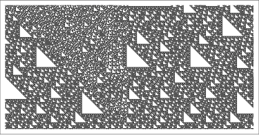
Figure 8. Spacetime diagram for the Ledrappier cellular automaton, whose generating polynomial is $\phi(x)=1+x^{-1}$, with a $2$-automatic initial condition generated by the substitution in Example 6.14. The dimensions are $511\times 256$.

Substitutions with coincidences are not the only ones which generate shift spaces contain the constant zero configuration. The next proposition identifies cellular automata and initial conditions which always give such a subshift.

Theorem 6.15.

Let $u\in\mathbb{F}_{p}^{\mathbb{Z}}$ be such that $(u_{m})_{m\geq 0}$ is $p$-automatic, and let $U=\operatorname*{ST}_{\Phi}(u)$. Let $\theta:\mathcal{A}\to\mathcal{A}^{p}$ and $\tau:\mathcal{A}\to\mathbb{F}_{p}$ be such that $(u_{m})_{m\geq 0}=\tau(\theta^{\infty}(a))$. Let $\Phi:\mathbb{F}_{p}^{\mathbb{Z}}\rightarrow\mathbb{F}_{p}^{\mathbb{Z}}$ be a linear cellular automaton of left radius $0$ with generating polynomial $\phi(x)=\sum_{i=0}^{r}\alpha_{i}x^{-i}\in\mathbb{F}_{p}[x^{-1}]$ such that $\sum_{i=0}^{r}\alpha_{i}=0$. If there exists a finite word $w=w_{0}w_{1}\cdots w_{r}\in\mathcal{A}^{r+1}$ such that $w$ occurs in $\theta^{\infty}(a)$ and $|\{w_{i}:\alpha_{i}\neq 0\}|=1$, then $X_{U}$ contains the constant zero configuration.

Proof.

Let $\{b\}=\{w_{i}:\alpha_{i}\neq 0\}$. For each $j\geq 0$, since $w$ occurs in $\theta^{\infty}(a)$, then $\theta^{j}(w)$ also occurs in $\theta^{\infty}(a)$. Also, for each $i$ in the interval $0\leq i\leq r$ such that $\alpha_{i}\neq 0$, $\theta^{j}(b)$ occurs at $\theta^{j}(w)_{[p^{j}i,p^{j}(i+1))}$. Since $\Phi^{p^{j}}$ has generating polynomial $\phi(x)^{p^{j}}=\sum_{i=0}^{r}\alpha_{i}x^{-p^{j}i}$, we have, for each $k$ in the interval $0\leq k<p^{j}$,

$$\left(\Phi^{p^{j}}\tau\left(\theta^{j}(w)\right)\right)_{k}=\sum_{i=0}^{r}\alpha_{i}\tau\left(\theta^{j}(w)_{p^{j}i+k}\right)=\sum_{i=0}^{r}\alpha_{i}\tau\left(\theta^{j}(b)_{k}\right)=\left(\sum_{i=0}^{r}\alpha_{i}\right)\tau\left(\theta^{j}(b)_{k}\right)=0,$$

so that the word $0^{p^{j}}$ occurs in $\operatorname*{ST}_{\Phi}(u)$. The result follows. ∎

We remark that in the previous proof, it is sufficient that the word $w$ occurs once in $\theta^{\infty}(a)$, since for each $j$ we obtain a triangular region of $0$’s. Also, appropriate versions of the previous two theorems could be stated without left radius $0$; then we would also need to specify the left side of the initial condition. Finally, given a $p$-automatic initial condition $u$, one can always find a linear cellular automaton $\Phi$ such that $\operatorname*{ST}_{\Phi}(u)$ contains arbitrarily large words which are identically zero. Conversely, given a linear cellular automaton $\Phi$ whose generating polynomial satisfies $\phi(1)=0$, one can find an initial condition such that $\operatorname*{ST}_{\Phi}(u)$ contains large words which are identically zero. Theorems 6.13 and 6.15 are useful tools in Section 6.1, where we wished to avoid finitely supported invariant measures.

Corollary 6.16.

Let $u\in\mathbb{F}_{2}^{\mathbb{Z}}$ be such that $(u_{m})_{m\geq 0}$ is $2$-automatic, and let $U=\operatorname*{ST}_{\Phi}(u)$. Let $\Phi:\mathbb{F}_{2}^{\mathbb{Z}}\rightarrow\mathbb{F}_{2}^{\mathbb{Z}}$ be the Ledrappier cellular automaton with generating polynomial $\phi(x)=1+x^{-1}\in\mathbb{F}_{2}[x^{-1}]$. Then $X_{U}$ contains the constant zero configuration.

Proof.

If $00$ or $11$ occurs in $(u_{m})_{m\geq 0}$, we are done by Theorem 6.15. Otherwise, $(u_{m})_{m\geq 0}$ is $0101\cdots$ or $1010\cdots$. Since each of these sequences has a coincidence, we are done by Theorem 6.13. ∎

Example 6.17.

Let $\Phi$ be the Ledrappier cellular automaton Let $\theta$ be the Thue–Morse substitution, $\theta(0)=01$ and $\theta(1)=10$, and let $p=2$. Then $00$ and $11$ occur in both fixed points of $\theta$ and the conditions of Corollary 6.16 are satisfied; see Figure 7.

References

- [1] Adamczewski, B., and Bell, J. P. Diagonalization and rationalization of algebraic Laurent series. Ann. Sci. Éc. Norm. Supér. (4) 46, 6 (2013), 963–1004.
- [2] Allouche, J.-P., and Berthé, V. Triangle de Pascal, complexité et automates. Bull. Belg. Math. Soc. Simon Stevin 4, 1 (1997), 1–23. Journées Montoises (Mons, 1994).
- [3] Allouche, J.-P., Deshouillers, J.-M., Kamae, T., and Koyanagi, T. Automata, algebraicity and distribution of sequences of powers. Ann. Inst. Fourier (Grenoble) 51, 3 (2001), 687–705.
- [4] Allouche, J.-P., and Shallit, J. Automatic Sequences: Theory, Applications, Generalizations. Cambridge University Press, Cambridge, 2003.
- [5] Allouche, J.-P., von Haeseler, F., Lange, E., Petersen, A., and Skordev, G. Linear cellular automata and automatic sequences. Parallel Comput. 23, 11 (1997), 1577–1592. Cellular automata (Gießen, 1996).
- [6] Allouche, J.-P., von Haeseler, F., Peitgen, H.-O., Petersen, A., and Skordev, G. Automaticity of double sequences generated by one-dimensional linear cellular automata. Theoret. Comput. Sci. 188, 1-2 (1997), 195–209.
- [7] Allouche, J.-P., von Haeseler, F., Peitgen, H.-O., and Skordev, G. Linear cellular automata, finite automata and Pascal’s triangle. Discrete Appl. Math. 66, 1 (1996), 1–22.
- [8] Aparicio Monforte, A., and Kauers, M. Formal Laurent series in several variables. Expo. Math. 31, 4 (2013), 350–367.
- [9] Arnoux, P., and Ito, S. Pisot substitutions and Rauzy fractals. Bull. Belg. Math. Soc. Simon Stevin 8, 2 (2001), 181–207. Journées Montoises d’Informatique Théorique (Marne-la-Vallée, 2000).
- [10] Bartlett, A. Spectral theory of substitutions. Ergodic Theory Dynam. Systems 38, 4 (2018), 1289–1341.
- [11] Berthé, V. Complexité et automates cellulaires linéaires. Theor. Inform. Appl. 34, 5 (2000), 403–423.
- [12] Bezuglyi, S., Kwiatkowski, J., Medynets, K., and Solomyak, B. Invariant measures on stationary Bratteli diagrams. Ergodic Theory Dynam. Systems 30, 4 (2010), 973–1007.
- [13] Bousquet-Mélou, M., and Petkov̌sek, M. Linear recurrences with constant coefficients: the multivariate case. Discrete Math. 225, 1-3 (2000), 51–75. Formal power series and algebraic combinatorics (Toronto, ON, 1998).
- [14] Boyle, M. Open problems in symbolic dynamics. In Geometric and probabilistic structures in dynamics, vol. 469 of Contemp. Math. Amer. Math. Soc., Providence, RI, 2008, pp. 69–118.
- [15] Charlier, E., Rampersad, N., and Shallit, J. Enumeration and decidable properties of automatic sequences. Internat. J. Found. Comput. Sci. 23, 5 (2012), 1035–1066.
- [16] Christol, G. Ensembles presque periodiques -reconnaissables. Theoret. Comput. Sci. 9, 1 (1979), 141–145.
- [17] Christol, G., Kamae, T., Mendès France, M., and Rauzy, G. Suites algébriques, automates et substitutions. Bull. Soc. Math. France 108, 4 (1980), 401–419.
- [18] Cobham, A. Uniform tag sequences. Math. Systems Theory 6 (1972), 164–192.
- [19] Cyr, V., and Kra, B. Nonexpansive -subdynamics and Nivat’s conjecture. Trans. Amer. Math. Soc. 367, 9 (2015), 6487–6537.
- [20] Cyr, V., and Kra, B. Free ergodic -systems and complexity. Proc. Amer. Math. Soc. 145, 3 (2017), 1163–1173.
- [21] Einsiedler, M. Invariant subsets and invariant measures for irreducible actions on zero-dimensional groups. Bull. London Math. Soc. 36, 3 (2004), 321–331.
- [22] Furstenberg, H. Disjointness in ergodic theory, minimal sets, and a problem in Diophantine approximation. Math. Systems Theory 1 (1967), 1–49.
- [23] Host, B., Maass, A., and Martínez, S. Uniform Bernoulli measure in dynamics of permutative cellular automata with algebraic local rules. Discrete Contin. Dyn. Syst. 9, 6 (2003), 1423–1446.
- [24] Kari, J., and Moutot, E. Nivat’s conjecture and pattern complexity in algebraic subshifts. Theoret. Comput. Sci. 777 (2019), 379–386.
- [25] Kitchens, B., and Schmidt, K. Markov subgroups of . In Symbolic dynamics and its applications (New Haven, CT, 1991), vol. 135 of Contemp. Math. Amer. Math. Soc., Providence, RI, 1992, pp. 265–283.
- [26] Massuir, A., Peltomäki, J., and Rigo, M. Automatic sequences based on Parry or Bertrand numeration systems. Adv. in Appl. Math. 108 (2019), 11–30.
- [27] Mossé, B. Puissances de mots et reconnaissabilité des points fixes d’une substitution. Theoret. Comput. Sci. 99, 2 (1992), 327–334.
- [28] Mousavi, H. Automatic theorem proving in Walnut. https://cs.uwaterloo.ca/~shallit/Papers/aut3.pdf.
- [29] Pivato, M. Ergodic theory of cellular automata. In Computational complexity. Vols. 1–6. Springer, New York, 2012, pp. 965–999.
- [30] Pivato, M., and Yassawi, R. Limit measures for affine cellular automata. Ergodic Theory Dynam. Systems 22, 4 (2002), 1269–1287.
- [31] Pivato, M., and Yassawi, R. The spatial structure of odometers in cellular automata. JAC 2008 (2009), 119–129.
- [32] Quas, A., and Zamboni, L. Periodicity and local complexity. Theoret. Comput. Sci. 319, 1-3 (2004), 229–240.
- [33] Rigo, M. Formal Languages, Automata and Numeration Systems 2: Applications to Recognizability and Decidability. Networks and Telecommunications Series. ISTE, London; John Wiley & Sons, Inc., Hoboken, NJ, 2014.
- [34] Rowland, E. IntegerSequences. https://github.com/ericrowland/IntegerSequences.
- [35] Rowland, E., and Yassawi, R. A characterization of -automatic sequences as columns of linear cellular automata. Adv. in Appl. Math. 63 (2015), 68–89.
- [36] Salon, O. Suites automatiques à multi-indices et algébricité. C. R. Acad. Sci. Paris Sér. I Math. 305, 12 (1987), 501–504.
- [37] Schmidt, K. Dynamical systems of algebraic origin, vol. 128 of Progress in Mathematics. Birkha̋user Verlag, Basel, 1995.
- [38] Silberger, S. Subshifts of the three dot system. Ergodic Theory Dynam. Systems 25, 5 (2005), 1673–1687.
- [39] Walters, P. An introduction to ergodic theory, vol. 79 of Graduate Texts in Mathematics. Springer-Verlag, New York-Berlin, 1982.