A least-squares functional for joint exit wave reconstruction and image registration

Abstract

Images generated by a transmission electron microscope (TEM) are blurred by aberrations from the objective lens and can be difficult to interpret correctly. One possible solution to this problem is to reconstruct the so-called exit wave, i.e. the electron wave in the microscope right before it passes the objective lens, from a series of TEM images acquired with varying focus. While the forward model of simulating a TEM image from a given exit wave is known and easy to evaluate, it is in general not possible to reconstruct the exit wave from a series of images analytically. The corresponding inverse problem can be formulated as a minimization problem, which is done in the well known MAL and MIMAP methods. We propose a generalization of these methods by performing the exit wave reconstruction and the registration of the image series simultaneously. We show that our objective functional is not convex with respect to the exit wave, which also carries over to the MAL and MIMAP functionals. The main result is the existence of minimizers of our objective functional. These results are based on the properties of a generalization of the cross-correlation. Finally, the applicability of our method is verified with a numerical experiment on simulated input data.

A definitive version of this manuscript was published in Inverse Problems, Volume 35, Number 5, 2019 and is available at https://dx.doi.org/10.1088/1361-6420/ab0b04

1 Introduction

In transmission electron microscopy (TEM), an image is generated by recording a beam of electrons that was transmitted through a sample, also called specimen. Due to diffraction inside the specimen, the electrons carry structural information when leaving the specimen at its exit plane. The electrons are then diverted by electromagnetic lenses to form an image in the image plane of the electron microscope.

There are several difficulties associated with directly interpreting TEM images. For instance, depending on the particular value of the objective lens aberrations at the time of image acquisition, entire atomic columns may not be visible in the recorded image or other features in the image may be mistakenly interpreted as atoms. These are the three main limitations inherent to TEM imaging:

1. The images are blurred by aberrations from the objective lens;

2. temporal and spatial partial coherence of the illumination; and

3. the phase of the image plane electron wave is missing in the images, since the microscope’s camera only records the squared amplitude of the electron wave.

Several approaches have been developed to deal with these limitations. These can be divided into two groups: improving the microscope’s hardware components [7, 12, 9, 18] and processing the TEM images [16, 3, 13, 4, 6].

One of the approaches on the image processing side is exit wave reconstruction, which aims to reconstruct the electron wave at the exit plane of the specimen, the so-called exit wave. The exit wave is most commonly reconstructed from a series of TEM images taken with varying focus of the objective lens; this way each of the real-valued images encodes a different portion of the complex-valued exit wave. Although the reconstructed exit wave is theoretically free from aberrations of the objective lens, in practice it is frequently necessary to correct residual aberrations [17]. This is due to the fact that the aberration coefficients are oftentimes not known to a high precision.

In this article, we investigate a generalization of two well-established variational methods for exit wave reconstruction: the multiple input maximum a-posteriori (MIMAP) algorithm [14] and the maximum-likelihood (MAL) algorithm [4]. In both algorithms, the exit wave is reconstructed by minimizing a functional of the kind

$$J_{\alpha}[\Psi]=\frac{1}{N}\sum_{j=1}^{N}\left|\left|\mathcal{I}_{\Psi,Z_{j}}^{\text{sim}}-\mathcal{I}_{j}^{\text{exp}}\right|\right|_{L^{2}}^{2}+\alpha\left|\left|\Psi-\Psi_{M}\right|\right|_{L^{2}}^{2},\qquad{\alpha\geq 0}.$$

It takes as input a finite series of experimental images $(\mathcal{I}_{j}^{\text{exp}})_{j=1,\ldots,N}$, which have been acquired with varying focus $(Z_{j})_{j=1,\ldots,N}$ of the objective lens. The experimental images are compared to simulated images $(\mathcal{I}_{\Psi,Z_{j}}^{\text{sim}})_{j=1,\ldots,N}$ that are calculated from an estimate of the exit wave $\Psi$ and the corresponding focus values $Z_{j}$. The parameter $\Psi_{M}$ is an a-priori estimate of the exit wave and is only used in the MIMAP algorithm, whereas $\alpha$ is equal to zero in the MAL algorithm. Minimizing the functional $J_{\alpha}$ corresponds to finding a (regularized) least squares approximation to the experimental input images. See, for example, [2] for an application of the MAL algorithm.

In principle, the exit wave can be reconstructed by only minimizing $J_{\alpha}$. As an initial guess, a constant exit wave corresponding to the square root of the mean image intensities or the results from one iteration of the paraboloid method may be used [4, 6]. However, due to specimen drift and microscope instabilities, an accurate registration of the experimental image series is necessary in addition to the minimization of $J_{\alpha}$. In the MAL algorithm as described in [4], this problem is solved in two steps. First, a rough initial alignment of the experimental images is computed by calculating the cross-correlation of subsequent images in the series. Second, after every iteration of the minimization method the alignment is further improved by calculating the cross-correlation of each experimental image with the corresponding simulated image. In the MIMAP algorithm the alignment is improved in every iteration by additionally applying a translation to the simulated images $\mathcal{I}_{\Psi,Z_{j}}^{\text{sim}}$ in the functional and minimizing the functional’s value with respect to this translation [14]. This is done without taking the update of the exit wave in the current iteration into account.

The generalization of the MAL and MIMAP algorithms we propose is to treat this as joint optimization problem, i.e. to optimize the exit wave and the registration simultaneously rather than alternatingly. The generalized functional is

$$E_{\alpha}[\Psi,t_{1},\ldots,t_{N}]=\frac{1}{N}\sum_{j=1}^{N}\left|\left|\mathcal{I}_{\Psi,Z_{j}}^{\text{sim}}-\mathcal{I}_{t_{j},j}^{\text{exp}}\right|\right|_{L^{2}}^{2}+\alpha\left|\left|\Psi-\Psi_{M}\right|\right|_{L^{2}}^{2}\qquad{\alpha\geq 0},$$

where $\mathcal{I}_{t_{j},j}^{\text{exp}}$ is the experimental image $\mathcal{I}_{j}^{\text{exp}}$ translated by $t_{j}\in\mathbb{R}^{2}$. This coupled treatment of the reconstruction with the registration is essential to our analysis of the existence of minimizers.

Carrying out such a mathematical analysis is the main contribution of this paper. To this end, we show that our objective functional is weakly lower semi-continuous and coercive, which enables us to proof the existence of minimizers with the direct method. Additionally, we show that our objective functional is in general not convex with respect to the exit wave. These results are fundamentally based on 1) a novel factorization property of the weight used in the forward model, which is given in Proposition 2.3, and 2) the notion of the weighted cross-correlation developed in Appendix A.

The structure of this article is as follows:

• The forward model: The simulation of a TEM image from a given exit wave amounts to calculating the weighted autocorrelation of the exit wave. In Section 2, the weight is introduced in detail and some of its properties are presented. The definition of the weighted cross-correlation is given in Appendix A, together with several generic properties independent of the application to exit wave reconstruction.

• The inverse problem: In Section 3, our objective functional for exit wave reconstruction and its derivatives are given. It is also shown that the functional is not convex with respect to the exit wave unless all experimental input images are zero.

• Existence of minimizers: The results from Appendix B suggest that the objective functional as given in Section 3 is not coercive. This problem is solved by adding a Tikhonov regularization term to the functional. Using the direct method, it is shown in Section 4 that minimizers of the regularized functional exist.

• Numerical experiment: We conclude with a numerical experiment on synthetic input data in Section 5, showing that our objective functional can indeed be used to reconstruct the exit wave and register the images simultaneously in practice.

Although this article is written from the point of view of exit wave reconstruction, the results are more generally applicable to any least-squares inverse problem where the forward model is a weighted autocorrelation as in Section 2. More precisely, the existence and convexity results still hold if the specific weight used for TEM image simulation is replaced with any weight that satisfies Lemmas 2.1, 2.2 and 2.3.

In the following, we frequently use the Fourier transform. Here, we use

$$\big{(}\mathcal{F}f\big{)}(x):=\int_{\mathbb{R}^{d}}f(y)e^{-2\pi\text{i}x\cdot y}\,\mathrm{d}y \forall\,x\in\mathbb{R}^{d}$$

as the definition of the Fourier transform of an integrable function $f\in L^{1}(\mathbb{R}^{d},\mathbb{C})$. This definition is convenient, since no additional scaling factor is needed when applying the convolution theorem. If the integration domain is omitted from an integral expression, the domain is always the entire vector space $\mathbb{R}^{d}$. Furthermore, all considered subsets of $\mathbb{R}^{d}$ are implicitly assumed to be Lebesgue measurable.

2 The forward model: simulating TEM images

The simulation of TEM images from a given exit wave and focus value is one of the core components of the inverse problem. In Fourier space, the simulated image $\mathcal{I}_{\Psi,Z}^{\text{sim}}\in L^{2}(\mathbb{R}^{2},\mathbb{C})$ is given by a weighted autocorrelation of the exit wave $\Psi\in L^{2}(\mathbb{R}^{2},\mathbb{C})$ [15]. Explicitly, we have

$$\mathcal{I}_{\Psi,Z}^{\text{sim}}=\Psi\star_{\widehat{T}_{Z}}\Psi,$$ (1)

where $Z\in\mathbb{R}$ is the focus value, $\widehat{T}_{Z}:\mathbb{R}^{2}\times\mathbb{R}^{2}\rightarrow\mathbb{C}$ is the transmission cross-coefficient (TCC), and $\Psi\star_{\widehat{T}_{Z}}\Psi$ denotes the weighted cross-correlation (cf. Definition A.1). Taking partial coherence into account, the TCC is defined as

$$\widehat{T}_{Z}:\mathbb{R}^{2}\times\mathbb{R}^{2}\rightarrow\mathbb{C},\;(v,w)\mapsto\int_{\mathbb{R}}\int_{\mathbb{R}^{2}}s(u)f(Z^{\prime})t_{Z+Z^{\prime}}(v+u)t_{Z+Z^{\prime}}^{*}(w+u)\,\mathrm{d}u\,\mathrm{d}Z^{\prime},$$ (2)

where $s\in L^{1}(\mathbb{R}^{2},\mathbb{R})$ and $f\in L^{1}(\mathbb{R},\mathbb{R})$ are probability density functions and $t_{Z}:\mathbb{R}^{2}\to\mathbb{C}$ is the pupil function. Here, $s$ is the normalized intensity distribution of the illumination and $f$ is the normalized focus spread. The pupil function is

$$t_{Z}(v):=p_{Z}(v)a(v) \forall\,v\in\mathbb{R}^{2}$$ ,

where $p_{Z}:\mathbb{R}^{2}\to\mathbb{C}$ is the pure phase transfer function and $a:\mathbb{R}^{2}\to\mathbb{R}$ is the aperture function.

The pure phase transfer function models the aberrations of the objective lens and is given by

$$p_{Z}(v):=\exp\big{(}-2\pi\text{i}\chi_{Z}(v)\big{)} \forall\,v\in\mathbb{R}^{2}$$ .

For the sake of simplicity, we only consider the two most important isotropic aberrations – focus and third order spherical aberration – in the wave aberration function $\chi_{Z}:\mathbb{R}^{2}\to\mathbb{R}$. Then

$$\chi_{Z}(v):=\frac{1}{2}Z\lambda\left|v\right|^{2}+\frac{1}{4}C_{s}\lambda^{3}\left|v\right|^{4} \forall\,v\in\mathbb{R}^{2}$$ ,

where $\lambda\in\mathbb{R}_{>0}$ is the electron wavelength and $C_{s}\in\mathbb{R}$ is the coefficient of the spherical aberration. Additional terms for higher order or anisotropic aberrations can easily be included in the wave aberration function. The general formula including all possible aberrations can e.g. be found in [15] or [19].

The aperture function models the objective aperture and is given by

$$a(v):=\begin{cases}1,&\text{if $\lambda\left|\left|v\right|\right|_{2}<\alpha_{\text{max}}$,}\\ 0,&\text{otherwise,}\end{cases} \forall\,v\in\mathbb{R}^{2}$$ ,

where $\lambda\in\mathbb{R}_{>0}$ is the electron wavelength and $\alpha_{\text{max}}\in\mathbb{R}_{>0}$ is the maximum semiangle allowed by the objective aperture. The set-theoretic support of the aperture function is a ball of radius $r_{a}:=\alpha_{\text{max}}/\lambda$ centered at the origin and is denoted by $A:=B_{\alpha_{\text{max}}/\lambda}(0)$.

Note that the pure phase transfer function $p_{Z}$ is continuous and the aperture function $a$ is bounded. The parameters $\lambda$, $C_{s}$ and $\alpha_{\text{max}}$ are treated as constants in the following.

Depending on the particular probability densities $s$ and $f$, the support of the TCC $\widehat{T}_{Z}$ might be unbounded. As a TCC with bounded support significantly simplifies the theory developed here, we will consider

$$T_{Z}(v,w):=a(v)a^{*}(w)\int_{\mathbb{R}}\int_{\mathbb{R}^{2}}s(u)f(Z^{\prime})p_{Z+Z^{\prime}}(v+u)p_{Z+Z^{\prime}}^{*}(w+u)\,\mathrm{d}u\,\mathrm{d}Z^{\prime}$$ (3)

instead of $\widehat{T}_{Z}$ in the following. In doing so, we ignored the dependency of the aperture function on the integration variable $u$. This is a common simplification that is justified if the diameter of the aperture is sufficiently large compared to the highest frequency of interest [15, 11, 8]. In particular, this can be considered as the first step towards Ishizuka’s well established approximation to the TCC $\widehat{T}_{Z}$ [11], which is used in the MAL and MIMAP algorithms.

Lemma 2.1 (Elementary properties of the TCC).

The transmission cross-coefficient $T_{Z}$ has the following properties:

1. $\left|T_{Z}(v,w)\right|\leq 1$ for all $v,w\in\mathbb{R}^{2}$,

2. $T_{Z}^{*}(v,w)=T_{Z}(w,v)$ for all $v,w\in\mathbb{R}^{2}$,

3. $T_{Z}(v,v)=1$ for all $v\in A$,

4. $T_{Z}(v,w)=0$ for all $v,w\in\mathbb{R}^{2}\backslash A$.

The second property has also been observed by Ishizuka in [11].

Proof.

All of the properties follow immediately from the definition of $T_{Z}$ and the properties of its components.∎

The first two properties of the TCC in Lemma 2.1 also hold for the more general version $\widehat{T}_{Z}$ of the TCC. In [11], it is shown that, as a direct consequence of the second property, the Fourier space image $G:=\mathcal{I}_{\Psi,Z}^{\text{sim}}$ satisfies Friedel’s law, i.e.

$$G(v)=G^{*}(-v) \forall\,v\in\mathbb{R}^{2}$$ .

Taking the inverse Fourier transform, this shows that the simulated image in real space is indeed real-valued, as one would expect from a TEM image.

An important property of the ordinary cross-correlation is that $f\star g$ is continuous for functions $f\in L^{p}(\mathbb{R}^{d})$ and $g\in L^{q}(\mathbb{R}^{d})$, where $d\in\mathbb{N}$ and $p,q>1$ with $\frac{1}{p}+\frac{1}{q}=1$. This property is generalized to weighted cross-correlations in Lemma A.8 on the additional assumption that the weight itself is continuous on a suitable open subset of $\mathbb{R}^{d}$.

Lemma 2.2 (Continuity of the TCC).

The transmission cross-coefficient $T_{Z}$ is continuous on $A\times A$.

Proof.

The integrand of $T_{Z}$ is dominated by the function $g\in L^{1}(\mathbb{R}^{2}\times\mathbb{R},\mathbb{R})$ defined as $g(u,Z^{\prime}):=\left|s(u)f(Z^{\prime})\right|$. Therefore, the result follows from the dominated convergence theorem and the continuity of $p_{Z}$.∎

If $(s_{n})_{n\in\mathbb{N}}\in L^{1}(\mathbb{R}^{2},\mathbb{R})^{\mathbb{N}}$ and $(f_{n})_{n\in\mathbb{N}}\in L^{1}(\mathbb{R},\mathbb{R})^{\mathbb{N}}$ are sequences of probability density functions with uniformly bounded support such that

$$\lim_{n\rightarrow\infty}\int_{B_{\varepsilon}(0)}s_{n}(u)\,\mathrm{d}u=1\qquad\text{and}\qquad\lim_{n\rightarrow\infty}\int_{(-\varepsilon,\varepsilon)}f_{n}(Z^{\prime})\,\mathrm{d}Z^{\prime}=1$$

for all $\varepsilon>0$, then

$$\lim_{n\rightarrow\infty}\lim_{m\rightarrow\infty} a(v)a^{*}(w)\int_{\mathbb{R}}\int_{\mathbb{R}^{2}}s_{n}(u)f_{m}(Z^{\prime})p_{Z+Z^{\prime}}(v+u)p_{Z+Z^{\prime}}^{*}(w+u)\,\mathrm{d}u\,\mathrm{d}Z^{\prime}$$

$$=\; a(v)a^{*}(w)p_{Z}(v)p_{Z}^{*}(w)=t_{Z}(v)t_{Z}^{*}(w)$$

for all $v,w\in\mathbb{R}^{2}$. This corresponds to the limiting case of perfect spatial and temporal coherence, in which the TCC is simply a product of the pupil function and its complex conjugate. In particular, the image simulation simplifies to

$$\mathcal{I}_{\Psi,Z}^{\text{sim}}=\Psi\star_{T_{Z}}\Psi=(\Psi t_{Z})\star(\Psi t_{Z})=(\Psi p_{Z}a)\star(\Psi p_{Z}a).$$

In the general case, there is no straightforward way to factorize the TCC and express $\Psi\star_{T_{Z}}\Psi$ as an ordinary cross-correlation. However, it is possible to approximate $T_{Z}$ by finite sums of factorizable functions, which is made precise in the following proposition. This factorization property will be most helpful for the analysis of the functional, as it enables us to apply the convolution theorem to weighted cross-correlations.

In the following, the integrand of the TCC is split into the two parts

$$g :\mathbb{R}^{2}\times\mathbb{R}\rightarrow\mathbb{R},\quad(u,Z^{\prime})\mapsto s(u)f(Z^{\prime}),$$

$$q_{v,w} :\mathbb{R}^{2}\times\mathbb{R}\rightarrow\mathbb{C},\quad(u,Z^{\prime})\mapsto p_{Z+Z^{\prime}}(v+u)p_{Z+Z^{\prime}}^{*}(w+u)$$

so that $T_{Z}(v,w)=a(v)a^{*}(w)\iint g(u,Z^{\prime})q_{v,w}(u,Z^{\prime})\,\mathrm{d}u\,\mathrm{d}Z^{\prime}$ for all $v,w\in\mathbb{R}^{2}$. Here, the supremum norm of a vector-valued function $\alpha:\mathbb{R}^{n}\rightarrow\mathbb{C}^{m}$ is defined as

$$\left|\left|\alpha\right|\right|_{\infty}:=\sup_{x\in\mathbb{R}^{n}}\left|\left|\alpha(x)\right|\right|_{\infty}.$$

Proposition 2.3 (Factorization property of the TCC).

Assume that $s$ and $f$ are differentiable with

$$\sup_{v,w\in A}\left|\left|g\nabla q_{v,w}\right|\right|_{\infty}<\infty\qquad\text{and}\qquad\left|\left|\nabla g\right|\right|_{\infty}<\infty.$$

Then there exists a sequence $(T_{Z,N})_{N\in\mathbb{N}}$ of functions converging uniformly to $T_{Z}$ with the following properties:

1. $T_{Z,N}$ is continuous and bounded on $A\times A$ and zero on $(\mathbb{R}^{2}\times\mathbb{R}^{2})\backslash(A\times A)$ for all $N\in\mathbb{N}$.

2. For all $N\in\mathbb{N}$, $j\in\{1,\ldots,N\}$ there are functions $t_{Z,N,j}:\mathbb{R}^{2}\rightarrow\mathbb{C}$ such that $t_{Z,N,j}$ is continuous and bounded on $A$, zero on $\mathbb{R}^{2}\backslash A$ and

   $$T_{Z,N}(v,w)=\sum_{j=1}^{N}t_{Z,N,j}(v)t_{Z,N,j}^{*}(w) \forall\,v,w\in\mathbb{R}^{2}$$ .

Proof.

Denote by

$$T_{Z}^{\prime}(v,w):=\int_{\mathbb{R}}\int_{\mathbb{R}^{2}}s(u)f(Z^{\prime})p_{Z+Z^{\prime}}(v+u)p_{Z+Z^{\prime}}^{*}(w+u)\,\mathrm{d}u\,\mathrm{d}Z^{\prime}$$

the TCC without the aperture function. As the integrand is continuous in $(u,Z^{\prime})$ and already factorized with respect to $v$ and $w$, we expect the Riemann sums

$$\sum_{\alpha=-M}^{M}\sum_{\beta,\gamma=-M}^{M}\underbrace{\delta_{M}\delta_{M}^{2}s(u_{\beta,\gamma})f(Z^{\prime}_{\alpha})}_{\geq 0}p_{Z+Z^{\prime}_{\alpha}}(v+u_{\beta,\gamma})p_{Z+Z^{\prime}_{\alpha}}^{*}(w+u_{\beta,\gamma}),$$

$$\bullet\;M\in\mathbb{N},$$

$$\bullet\;\delta_{M}=M^{-k}\quad\text{for $k\in\big{(}\tfrac{3}{4},1\big{)}$},$$

$$\bullet\;u_{\beta,\gamma}=(\beta\delta_{M},\gamma\delta_{M})\in\mathbb{R}^{2},$$

$$\bullet\;Z_{\alpha}^{\prime}=\alpha\delta_{M}\in\mathbb{R}$$

to be suitable approximations of $T_{Z}^{\prime}$ as sums of factorizable functions. If we define

$$t_{Z,M,\alpha,\beta,\gamma}(v):=a(v)\sqrt{\delta_{M}\delta_{M}^{2}s(u_{\beta,\gamma})f(Z^{\prime}_{\alpha})}p_{Z+Z^{\prime}_{\alpha}}(v+u_{\beta,\gamma}) \forall\,v\in\mathbb{R}^{2}$$ ,

then reordering the indices $\alpha,\beta,\gamma\in\{-M,\ldots,M\}$ to a single index $j\in\{1,\ldots,N\}$ yields the sought functions $t_{Z,N,j}$. It remains to show that the sums converge uniformly to $T_{Z}^{\prime}$ on $A\times A$ as $M\rightarrow\infty$, since the aperture function is zero on $\mathbb{R}^{2}\backslash A$.

Let $\varepsilon>0$ and fix $v,w\in A$. First, we note that the integrand

$$h_{v,w}:\mathbb{R}^{2}\times\mathbb{R}\rightarrow\mathbb{C},\quad(u,Z^{\prime})\mapsto s(u)f(Z^{\prime})p_{Z+Z^{\prime}}(v+u)p_{Z+Z^{\prime}}^{*}(w+u)$$

is Lipschitz continuous. This follows from the fact that the gradient is bounded by

$$\left|\left|\nabla h_{v,w}\right|\right|_{\infty} =\left|\left|\nabla(gq_{v,w})\right|\right|_{\infty}=\left|\left|g\nabla q_{v,w}+q_{v,w}\nabla g\right|\right|_{\infty}\leq\left|\left|g\nabla q_{v,w}\right|\right|_{\infty}+\left|\left|\nabla g\right|\right|_{\infty}$$

$$\leq\sup_{v,w\in A}\left|\left|g\nabla q_{v,w}\right|\right|_{\infty}+\left|\left|\nabla g\right|\right|_{\infty}=:L<\infty.$$

Let $J_{M}:=[-M\delta_{M},(M+1)\delta_{M}]$ and $I_{x}:=[x\delta_{M},(x+1)\delta_{M}]$ for all $x\in\mathbb{Z}$, $M\in\mathbb{N}$. Using the triangle inequality,

$$\phantom{=}\left|\sum_{\alpha=-M}^{M}\sum_{\beta,\gamma=-M}^{M}\delta_{M}^{3}h_{v,w}(u_{\beta,\gamma},Z^{\prime}_{\alpha})-\int_{\mathbb{R}}\int_{\mathbb{R}^{2}}h_{v,w}(u,Z^{\prime})\,\mathrm{d}u\,\mathrm{d}Z^{\prime}\right|$$

$$\leq\left|\sum_{\alpha=-M}^{M}\sum_{\beta,\gamma=-M}^{M}\delta_{M}^{3}h_{v,w}(u_{\beta,\gamma},Z^{\prime}_{\alpha})-\int_{J_{M}}\int_{J_{M}\times J_{M}}h_{v,w}(u,Z^{\prime})\,\mathrm{d}u\,\mathrm{d}Z^{\prime}\right|+C_{M}$$

$$\leq\sum_{\alpha=-M}^{M}\sum_{\beta,\gamma=-M}^{M}\int_{I_{\alpha}}\int_{I_{\beta}\times I_{\gamma}}\left|h_{v,w}(u_{\beta,\gamma},Z^{\prime}_{\alpha})-h_{v,w}(u,Z^{\prime})\right|\,\mathrm{d}u\,\mathrm{d}Z^{\prime}+C_{M}$$

$$\leq\sum_{\alpha=-M}^{M}\sum_{\beta,\gamma=-M}^{M}\int_{I_{\alpha}}\int_{I_{\beta}\times I_{\gamma}}3L\left|\left|(u_{\beta,\gamma},Z_{\alpha}^{\prime})-(u,Z^{\prime})\right|\right|_{\infty}\,\mathrm{d}u\,\mathrm{d}Z^{\prime}+C_{M}$$

$$\leq(2M+1)^{3}\delta_{M}^{3}\cdot 3L\delta_{M}+C_{M},$$ (4)

where $C_{M}=\sup_{v,w\in A}\int_{\mathbb{R}^{3}\backslash J_{M}^{3}}\left|h_{v,w}(x)\right|\,\mathrm{d}x$. The functions

$$c_{M}:\overline{A}\times\overline{A}\rightarrow\mathbb{R},\quad(v,w)\mapsto\int_{\mathbb{R}^{3}\backslash J_{M}^{3}}\left|h_{v,w}(x)\right|\,\mathrm{d}x\qquad(M\in\mathbb{N})$$

define a monotone sequence of continuous functions, which converges pointwise to zero on the compact space $\overline{A}\times\overline{A}$. Hence $c_{M}$ converges uniformly to zero as $M\rightarrow\infty$ by Dini’s theorem, which implies $\lim_{M\rightarrow\infty}C_{M}=0$. The first summand in Equation 4 also converges to zero for $M\rightarrow\infty$, since $\delta_{M}=M^{-k}$ with $k\in(\frac{3}{4},1)$. This shows the uniform convergence of the Riemann sums to $T_{Z}^{\prime}$ on $A\times A$.∎

Intuitively, the assumption $\sup_{v,w\in A}\left|\left|g\nabla q_{v,w}\right|\right|_{\infty}<\infty$ ensures that $s$ and $f$ decrease at least as fast as the gradient of $q_{v,w}$ grows. For instance, if $s$ and $f$ are Gaussian probability densities, then this condition is clearly fulfilled as $\nabla q_{v,w}$ grows only polynomially.

Using the factorization property of $T_{Z}$, it is shown in the following corollary that $\mathcal{F}^{-1}(\mathcal{I}_{\Psi,Z}^{\text{sim}})$ is not only real-valued, but also nonnegative. This is clearly a desired property of the simulation, since TEM images consist of electron counts and thus should not contain negative values.

Corollary 2.4.

The simulated real space images $\mathcal{F}^{-1}(\mathcal{I}_{\Psi,Z}^{\text{sim}})=\mathcal{F}^{-1}(\Psi\star_{T_{Z}}\Psi)$ are nonnegative for all $\Psi\in L^{2}(\mathbb{R}^{2},\mathbb{C})$.

Proof.

By Proposition 2.3, the TCC is an element of $W^{+}(\mathbb{R}^{2})$ (cf. Appendix A). Combining the elementary properties from Lemma 2.1 with Lemma A.6 therefore shows that $\mathcal{F}^{-1}(\Psi\star_{T_{Z}}\Psi)\geq 0$ for all $\Psi\in L^{2}(\mathbb{R}^{2},\mathbb{C})$. ∎

For the remainder of this section, we describe how the forward model from the MAL and MIMAP algorithms fits into the framework described here. There, an image is simulated using Equation 1 with Ishizuka’s TCC [11] instead of $\widehat{T}_{Z}$ or $T_{Z}$. Ishizuka’s TCC is an approximation to $T_{Z}$ that makes two assumptions for numerical efficiency:

1. the use of a high resolution TEM to investigate a weakly scattering object;

2. the intensity distribution of the illumination $s$ and the focus spread $f$ can be modeled by Gaussian probability densities.

Using these assumptions, the TCC $T_{Z}$ is simplified to yield

$$T_{Z}^{\text{Ishizuka}}(v,w):=p_{Z}(v)p_{Z}^{*}(w)a(v)a^{*}(w)E_{s}(v,w)E_{t}(v,w),$$ (5)

where $E_{s}$ and $E_{t}$ are damping envelopes that model the effects of partial spatial and temporal coherence respectively. They are given by

$$E_{s}(v,w) :=\exp\left(-\left(\frac{\pi\alpha}{\lambda}\right)^{2}\left|\nabla\chi(v)-\nabla\chi(w)\right|^{2}\right),$$

$$E_{t}(v,w) :=\exp\left(-\frac{1}{2}(\pi\Delta\lambda)^{2}\left(\left|v\right|^{2}-\left|w\right|^{2}\right)^{2}\right),$$

where $\lambda\in\mathbb{R}_{>0}$ is the electron wavelength, $\alpha\in\mathbb{R}_{\geq 0}$ is the half angle of beam convergence and $\Delta\in\mathbb{R}_{\geq 0}$ is the focus spread parameter.

The factorization property given in Proposition 2.3 is related to the focal integration approximation that is used in the MAL algorithm. There, the temporal coherence envelope $E_{t}$ is approximated by a sum of factorizable terms that originate from a numerical integration of

$$E_{t}(v,w) =\int_{-\infty}^{\infty}f_{\Delta}(x)\exp\left(-\pi\text{i}\lambda x\left(\left|v\right|^{2}-\left|w\right|^{2}\right)\right)\,\mathrm{d}x,$$ (6)

$$f_{\Delta}(x) =\frac{1}{\sqrt{2\pi}\Delta}\exp\left(-\frac{x^{2}}{2\Delta^{2}}\right),$$

where $f_{\Delta}$ is the focus spread. This integral expression is equal to the original definition of $E_{t}$, since

$$\exp(-C^{2})=\int_{-\infty}^{\infty}\frac{1}{\sqrt{\pi}}\exp(-2\text{i}Cx)\exp(-x^{2})\,\mathrm{d}x$$

holds for all $C\in\mathbb{R}$. For practical reasons, the spatial coherence envelope $E_{s}$ is only roughly approximated by $E_{s}(v,w)\approx E_{s}(v,0)E_{s}^{*}(w,0)$ in the MAL algorithm. Therefore, the approximations to the TCC used in the MAL algorithm do not converge to $T_{Z}^{\text{Ishizuka}}$. However, if the spatial coherence envelope is instead expressed as

$$E_{s}(v,w) =\prod_{j=1}^{2}\exp\left(-\left(\frac{\pi\alpha}{\lambda}\right)^{2}\left|\partial_{j}\chi(v)-\partial_{j}\chi(w)\right|^{2}\right)$$

$$=\prod_{j=1}^{2}\int_{-\infty}^{\infty}\frac{1}{\sqrt{\pi}\alpha}\exp\left(-\frac{x^{2}}{\alpha^{2}}\right)\exp\left(-\frac{2\pi ix}{\lambda}\left(\partial_{j}\chi_{Z}(v)-\partial_{j}\chi_{Z}(w)\right)\right)\,\mathrm{d}x,$$ (7)

then a numerical integration of Equations 6 and 2 yields approximations to $T_{Z}^{\text{Ishizuka}}$ as sums of factorizable functions. It can be shown that these approximations converge uniformly, so the approximation property in Proposition 2.3 also holds for Ishizuka’s TCC.

From the definition of $T_{Z}^{\text{Ishizuka}}$ in Equation 5 it is clear that Lemma 2.2 continues to hold as well as all of the elementary properties given in Lemma 2.1.

3 The objective functional

In this section, our objective functional for exit wave reconstruction and its derivatives are given, alongside with a result regarding the convexity of the objective functional. By the results of the previous section, the statements in this section still hold if the TCC $T_{Z}$ is replaced with $T_{Z}^{\text{Ishizuka}}$.

Definition 3.1.

Let $N\in\mathbb{N}$ and $g_{1},\ldots,g_{N}\in L^{1}(\mathbb{R}^{2},\mathbb{R}_{\geq 0})\cap L^{2}(\mathbb{R}^{2},\mathbb{R}_{\geq 0})$ be a series of real space TEM images such that $\operatorname{supp}(\mathcal{F}(g_{j}))\subseteq\overline{2A}$ for all $j\in\{1,\ldots,N\}$. Denote by $Z_{j}\in\mathbb{R}$ the focus value associated with the image $g_{j}$. The objective functional for joint reconstruction and registration is defined as

$$E:L^{2}(A,\mathbb{C})\times(\mathbb{R}^{2})^{N}\rightarrow\mathbb{R},\quad(\Psi,t)\mapsto\frac{1}{N}\sum_{j=1}^{N}\big{|}\big{|}\Psi\star_{T_{Z_{j}}}\Psi-\mathcal{F}(g_{j}\circ\phi_{t_{j}})\big{|}\big{|}_{L^{2}}^{2},$$ (8)

where $\phi_{y}:\mathbb{R}^{2}\rightarrow\mathbb{R}^{2},\;x\mapsto x+y$ is the translation by $y\in\mathbb{R}^{2}$. Here, $I_{\Psi,Z_{j}}^{\text{sim}}=\Psi\star_{T_{Z_{j}}}\Psi$ are the simulated images in Fourier space and $I_{t_{j},j}^{\text{exp}}=\mathcal{F}(g_{j}\circ\phi_{t_{j}})$ are the translated experimental images in Fourier space.

The regularization term $\alpha\left|\left|\Psi-\Psi_{M}\right|\right|_{L^{2}}^{2}$ presented in the introduction is not relevant in this section and therefore will only be added to our objective functional in Section 4.

The functional is well-defined, because $\Psi\star_{T_{Z_{j}}}\Psi\in L^{2}(\mathbb{R}^{2},\mathbb{C})$ by Corollary A.4 and clearly also $\mathcal{F}(g_{j}\circ\phi_{t_{j}})\in L^{2}(\mathbb{R}^{2},\mathbb{C})$ for all $j\in\{1,\ldots,N\}$. The domain of the exit wave is restricted to $A$, since all frequencies outside of $A$ are filtered out due to

$$\Psi\star_{T_{Z_{j}}}\Psi=(\Psi a)\star_{T_{Z_{j}}}(\Psi a)$$ (9)

and therefore do not contribute to the simulated images. Equation 9 follows from the fact that the aperture function satisfies $a(v)^{2}=a(v)$ for all $v\in\mathbb{R}^{2}$. The additional restriction $\operatorname{supp}(\mathcal{F}(g_{j}))\subseteq\overline{2A}$ on the frequencies of the experimental images does not affect the reconstruction, since $\operatorname{supp}(\Psi\star_{T_{Z}}\Psi)\subseteq\overline{2A}$ for all $\Psi\in L^{2}(A,\mathbb{C}),Z\in\mathbb{R}$ and $\operatorname{supp}(\mathcal{F}(g_{j}\circ\phi_{y}))=\operatorname{supp}(\mathcal{F}(g_{j}))$ for all $y\in\mathbb{R}^{2}$. Thus only image plane frequencies $v$ with $\left|v\right|<2r_{a}$, where $r_{a}$ is the aperture radius, can be reconstructed with the objective functional. Hence a low-pass filter of radius $2r_{a}$ may be applied to the experimental input images $g_{1},\ldots,g_{N}$ without loss of generality.

Note that a translation in real space can be expressed as a modulation in Fourier space by means of the identity

$$\mu_{y}\mathcal{F}(g)=\mathcal{F}(g\circ\phi_{y}),$$

which holds for all $g\in L^{1}(\mathbb{R}^{2},\mathbb{R})$ and $y\in\mathbb{R}^{2}$, where $\mu_{y}:\mathbb{R}^{2}\rightarrow\mathbb{C},\;x\mapsto e^{2\pi ix\cdot y}$ is the modulation by $y$. Therefore, the objective functional in Equation 8 can be written as

$$E:L^{2}(A,\mathbb{C})\times(\mathbb{R}^{2})^{N}\rightarrow\mathbb{R},\quad(\Psi,t)\mapsto\frac{1}{N}\sum_{j=1}^{N}\big{|}\big{|}\Psi\star_{T_{Z_{j}}}\Psi-\mu_{t_{j}}\mathcal{F}(g_{j})\big{|}\big{|}_{L^{2}}^{2}.$$

With this variant of the objective functional it can be seen that the translation may equivalently be applied to the exit wave instead of the experimental images. This follows from

$$\Big{(}(\Psi\mu_{y})\star_{T_{Z_{j}}}(\Psi\mu_{y})\Big{)}(x) =\int_{\mathbb{R}^{2}}\Psi^{*}(z)\mu_{y}^{*}(z)\Psi(x+z)\mu_{y}(x+z)T_{Z_{j}}(x+z,z)\,\mathrm{d}z$$

$$=\int_{\mathbb{R}^{2}}e^{2\pi ix\cdot y}\Psi^{*}(z)\Psi(x+z)T_{Z_{j}}(x+z,z)\,\mathrm{d}z$$

$$=\mu_{y}(x)\Big{(}\Psi\star_{T_{Z_{j}}}\Psi\Big{)}(x),$$

which implies

$$\frac{1}{N}\sum_{j=1}^{N}\big{|}\big{|}\Psi\star_{T_{Z_{j}}}\Psi-\mu_{t_{j}}\mathcal{F}(g_{j})\big{|}\big{|}_{L^{2}}^{2}=\frac{1}{N}\sum_{j=1}^{N}\big{|}\big{|}(\Psi\mu_{-t_{j}})\star_{T_{Z_{j}}}(\Psi\mu_{-t_{j}})-\mathcal{F}(g_{j})\big{|}\big{|}_{L^{2}}^{2}.$$

The right-hand side of the above equation is essentially identical to the functional that is used in the MIMAP algorithm for the optimization of the registration [14]. Therefore, the MIMAP algorithm can be considered as a special case of our joint optimization approach.

Equation 8 can be regarded as the Fourier space formulation of $E$. Since the Fourier transform is unitary, the equivalent real space formulation of the objective functional is

$$E[\Psi,t]=\frac{1}{N}\sum_{j=1}^{N}\big{|}\big{|}\mathcal{F}^{-1}\big{(}\Psi\star_{T_{Z_{j}}}\Psi\big{)}-g_{j}\circ\phi_{t_{j}}\big{|}\big{|}_{L^{2}}^{2}.$$

In the MAL algorithm, the exit wave is reconstructed by alternatingly minimizing the MAL functional

$$E_{\text{MAL}}[\Psi]=\frac{1}{N}\sum_{j=1}^{N}\big{|}\big{|}\Psi\star_{T_{Z_{j}}^{\text{Ishizuka}}}\Psi-\mathcal{F}(g_{j})\big{|}\big{|}_{L^{2}}^{2}$$

and updating the registration, where the registration is updated using the cross-correlation of simulated and experimental images. Interestingly, the MAL algorithm is equivalent to alternatingly minimizing our objective functional with respect to $\Psi$ and $t$, which can be seen as follows.

On the one hand, if $t=0$ is fixed, then $E[\Psi,t]=E_{\text{MAL}}[\Psi]$ for all $\Psi\in L^{2}(A,\mathbb{C})$ and it is clear that minimizing $E$ with respect to $\Psi$ is equivalent to minimizing $E_{\text{MAL}}$. On the other hand, if $\Psi$ is fixed, consider the real space formulation of $E$ and define $f_{\Psi,j}:=\mathcal{F}^{-1}\big{(}\Psi\star_{T_{Z_{j}}}\Psi\big{)}$ for all $j\in\{1,\ldots,N\}$. Minimizing

$$E[\Psi,t]=\frac{1}{N}\sum_{j=1}^{N}\left|\left|f_{\Psi,j}-g_{j}\circ\phi_{t_{j}}\right|\right|_{L^{2}}^{2}=\frac{1}{N}\sum_{j=1}^{N}\left|\left|f_{\Psi,j}\right|\right|_{L^{2}}^{2}+\left|\left|g_{j}\right|\right|_{L^{2}}^{2}-2\left(f_{\Psi,j},g_{j}\circ\phi_{t_{j}}\right)_{L^{2}}$$

with respect to $t$ is equivalent to maximizing

$$\left(f_{\Psi,j},g_{j}\circ\phi_{t_{j}}\right)_{L^{2}}=\int_{\mathbb{R}^{2}}f_{\Psi,j}(y)g_{j}(y+t_{j})\,\mathrm{d}y=\big{(}f_{\Psi,j}\star g_{j}\big{)}(t_{j})$$

for all $j\in\{1,\ldots,N\}$. The latter is precisely the method used in the MAL algorithm to update the registration.

Remark:

Aside from the reconstruction and registration, a minimizer of $E$ also yields denoised approximations $\mathcal{F}^{-1}\big{(}\Psi\star_{T_{Z_{j}}}\Psi\big{)}$ to the input images for two reasons. On the one hand, a minimizer is a least squares approximation according to the definition of $E$, which therefore averages the experimental images. On the other hand, the simulated real space images $\mathcal{F}^{-1}(\Psi\star_{T_{Z}}\Psi)$ are smooth, which can be seen as follows.

Because of the aperture function and Lemma A.2, the simulated Fourier space images $\Psi\star_{T_{Z}}\Psi$ are compactly supported and bounded for all $\Psi\in L^{2}(A,\mathbb{C})$ and all $Z\in\mathbb{R}$. By the dominated convergence theorem, the partial derivatives are therefore given by

$$\frac{\partial^{n}}{\partial x^{n}}\mathcal{F}^{-1}\big{(}\Psi\star_{T_{Z}}\Psi\big{)}(x)=\int_{\mathbb{R}^{2}}\big{(}\Psi\star_{T_{Z}}\Psi\big{)}(y)\frac{\partial^{n}}{\partial x^{n}}e^{2\pi\text{i}x\cdot y}\,\mathrm{d}y$$

for all $n\in\mathbb{N}_{0}^{2}$.

Using the notation and elementary properties of the weighted cross-correlation from Appendix A, it is easily shown that $\Psi\mapsto E[\Psi,t]$ restricted to any one-dimensional affine subspace of its domain $L^{2}(A,\mathbb{C})$ is a polynomial of degree $4$:

Lemma 3.2.

Let $t\in(\mathbb{R}^{2})^{N}$. For all $\Psi,\Phi\in L^{2}(A,\mathbb{C})$ with $\Phi\neq 0$ there are coefficients $\big{(}C_{\Psi,\Phi,t}^{j}\big{)}_{j=0,\ldots,4}\in\mathbb{R}^{5}$ with

$$E[\Psi+\alpha\Phi,t]=\sum_{j=0}^{4}C_{\Psi,\Phi,t}^{j}\alpha^{j}$$

for all $\alpha\in\mathbb{R}$. Furthermore, $C_{\Psi,\Phi,t}^{4}>0$.

Proof.

Denote the modulated input images by $G_{j}:=\mu_{t_{j}}\mathcal{F}(g_{j})$. Then,

$$E[\Psi+\alpha\Phi,t]=\frac{1}{N}\sum_{j=1}^{N}\left|\left|(\Psi+\alpha\Phi)\star_{T_{Z_{j}}}(\Psi+\alpha\Phi)-G_{j}\right|\right|_{L^{2}}^{2}$$

$$=\frac{1}{N}\sum_{j=1}^{N}\left|\left|\Psi\star_{T_{Z_{j}}}\Psi-G_{j}+\alpha(\Psi\star_{T_{Z_{j}}}\Phi+\Phi\star_{T_{Z_{j}}}\Psi)+\alpha^{2}(\Phi\star_{T_{Z_{j}}}\Phi)\right|\right|_{L^{2}}^{2}$$

for all $\alpha\in\mathbb{R}$. Expanding and collecting coefficients with the same power of $\alpha$ yields $E[\Psi+\alpha\Phi,t]=\sum_{j=0}^{4}C_{\Psi,\Phi,t}^{j}\alpha^{j}$ with

$$C_{\Psi,\Phi,t}^{0} =\frac{1}{N}\sum_{j=1}^{N}\left|\left|\Psi\star_{T_{Z_{j}}}\Psi-G_{j}\right|\right|_{L^{2}}^{2},$$

$$C_{\Psi,\Phi,t}^{1} =\frac{2}{N}\sum_{j=1}^{N}\mathrm{Re}\Big{(}\big{(}\Psi\star_{T_{Z_{j}}}\Psi-G_{j},\Psi\star_{T_{Z_{j}}}\Phi+\Phi\star_{T_{Z_{j}}}\Psi\big{)}_{L^{2}}\Big{)},$$

$$C_{\Psi,\Phi,t}^{2} =\frac{1}{N}\sum_{j=1}^{N}\left|\left|\Psi\star_{T_{Z_{j}}}\Phi+\Phi\star_{T_{Z_{j}}}\Psi\right|\right|_{L^{2}}^{2}+2\mathrm{Re}\Big{(}\big{(}\Psi\star_{T_{Z_{j}}}\Psi-G_{j},\Phi\star_{T_{Z_{j}}}\Phi\big{)}_{L^{2}}\Big{)},$$

$$C_{\Psi,\Phi,t}^{3} =\frac{2}{N}\sum_{j=1}^{N}\mathrm{Re}\Big{(}\big{(}\Psi\star_{T_{Z_{j}}}\Phi+\Phi\star_{T_{Z_{j}}}\Psi,\Phi\star_{T_{Z_{j}}}\Phi\big{)}_{L^{2}}\Big{)},$$

$$C_{\Psi,\Phi,t}^{4} =\frac{1}{N}\sum_{j=1}^{N}\left|\left|\Phi\star_{T_{Z_{j}}}\Phi\right|\right|_{L^{2}}^{2}.$$

Using the symmetry properties in Lemma A.5 and the fact that $G_{j}(v)=G_{j}^{*}(-v)$ for all $v\in\mathbb{R}^{2}$, the coefficients of the odd powers of $\alpha$ can be simplified to

$$C_{\Psi,\Phi,t}^{1} =\frac{4}{N}\sum_{j=1}^{N}\mathrm{Re}\Big{(}\big{(}\Psi\star_{T_{Z_{j}}}\Psi-G_{j},\Psi\star_{T_{Z_{j}}}\Phi\big{)}_{L^{2}}\Big{)},$$

$$C_{\Psi,\Phi,t}^{3} =\frac{4}{N}\sum_{j=1}^{N}\mathrm{Re}\Big{(}\big{(}\Psi\star_{T_{Z_{j}}}\Phi,\Phi\star_{T_{Z_{j}}}\Phi\big{)}_{L^{2}}\Big{)}.$$

The coefficient $C_{\Psi,\Phi,t}^{4}$ is positive by Lemma A.9.∎

The Gâteaux differentials of $E$ with respect to $\Psi$ can now simply be read off the polynomials’ coefficients.

Corollary 3.3.

Let $t\in(\mathbb{R}^{2})^{N}$ and $\Psi,\Phi\in L^{2}(A,\mathbb{C})$ with $\Phi\neq 0$. The Gâteaux differentials of $E$ at $(\Psi,t)$ in the direction $(\Phi,0)$ are

$$\big{\langle}\partial_{\Psi}E^{(n)}[\Psi,t],\Phi\big{\rangle}:=\left.\frac{d}{d\varepsilon}\big{\langle}\partial_{\Psi}E^{(n-1)}[\Psi+\varepsilon\Phi,t],\Phi\big{\rangle}\right|_{\varepsilon=0}=\begin{cases}n!C_{\Psi,\Phi,t}^{n},&n\in\{1,\ldots,4\},\\ 0,&n\geq 5.\end{cases}$$

The first order Gâteaux differential of $E$ with respect to the translation $t$ is calculated more directly without using difference quotients:

Lemma 3.4.

Let $\Psi\in L^{2}(A,\mathbb{C})$ and $t,\tilde{t}\in(\mathbb{R}^{2})^{N}$ with $\tilde{t}\neq 0$. The first order Gâteaux differential of $E$ at $(\Psi,t)$ in the direction $(0,\tilde{t})$ is

$$\big{\langle}\partial_{t}E[\Psi,t],\tilde{t}\big{\rangle}=-\frac{2}{N}\sum_{j=1}^{N}\mathrm{Re}\left(\big{(}\Psi\star_{T_{Z_{j}}}\Psi-\mu_{t_{j}}\mathcal{F}(g_{j}),\nu_{\tilde{t}_{j}}\mu_{t_{j}}\mathcal{F}(g_{j})\big{)}_{L^{2}}\right),$$

where $\nu_{\tilde{t}_{j}}(x)=2\pi ix\cdot\tilde{t}_{j}$ for all $x\in\mathbb{R}^{2}$.

Proof.

By the definition of $E$, we have

$$\big{\langle}\partial_{t}E[\Psi,t],\tilde{t}\big{\rangle}=\frac{1}{N}\sum_{j=1}^{N}\frac{d}{d\varepsilon}\int_{\mathbb{R}^{2}}\Big{|}\underbrace{(\Psi\star_{T_{Z_{j}}}\Psi)(x)-\mu_{t_{j}+\varepsilon\tilde{t}_{j}}(x)\mathcal{F}(g_{j})(x)}_{=:R_{j,\varepsilon}(x)}\left.\Big{|}^{2}\,\mathrm{d}x\right|_{\varepsilon=0}.$$

The partial derivative of the integrand is given by

$$\frac{d}{d\varepsilon}\left|R_{j,\varepsilon}(x)\right|^{2}=\frac{d}{d\varepsilon}\left(R_{j,\varepsilon}(x)R_{j,\varepsilon}^{*}(x)\right)=2\mathrm{Re}\left(\left(\frac{d}{d\varepsilon}R_{j,\varepsilon}(x)\right)R_{j,\varepsilon}^{*}(x)\right),$$

where

$$\frac{d}{d\varepsilon}R_{j,\varepsilon}(x)=-\nu_{\tilde{t}_{j}}(x)\mu_{t_{j}+\varepsilon\tilde{t}_{j}}(x)\mathcal{F}(g_{j})(x).$$

This derivative is dominated by

$$\left|\frac{d}{d\varepsilon}\left|R_{j,\varepsilon}(x)\right|^{2}\right|\leq 2\big{|}\nu_{\tilde{t}_{j}}(x)\big{|}\left|\mathcal{F}(g_{j})(x)\right|\left(\left|\big{(}\Psi\star_{T_{Z_{j}}}\Psi\big{)}(x)\right|+\left|\mathcal{F}(g_{j})(x)\right|\right)$$

for all $\varepsilon>0$, which is an integrable function by the Cauchy-Schwarz inequality, Corollary A.4 and Definition 3.1. This implies

$$\big{\langle}\partial_{t}E[\Psi,t],\tilde{t}\big{\rangle} =\frac{1}{N}\sum_{j=1}^{N}\int_{\mathbb{R}^{2}}\frac{d}{d\varepsilon}\left.\left|R_{j,\varepsilon}(x)\right|^{2}\right|_{\varepsilon=0}\,\mathrm{d}x$$

$$=-\frac{2}{N}\sum_{j=1}^{N}\mathrm{Re}\left(\big{(}\Psi\star_{T_{Z_{j}}}\Psi-\mu_{t_{j}}\mathcal{F}(g_{j}),\nu_{\tilde{t}_{j}}\mu_{t_{j}}\mathcal{F}(g_{j})\big{)}_{L^{2}}\right).$$ ∎

It is apparent that $E$ is not convex with respect to $t$ for arbitrary image series $(g_{j})_{j=1,\ldots,N}$. The following proposition shows that $E$ is also not convex with respect to $\Psi$.

Proposition 3.5.

Let $t\in(\mathbb{R}^{2})^{N}$. If $g_{j}\neq 0$ for at least one $j\in\{1,\ldots,N\}$, then $\Psi\mapsto E[\Psi,t]$ is not convex.

Proof.

Assume that at least one image $g_{j}$ is nonzero. We consider $\Psi\mapsto E[\Psi,t]$ restricted to the lines in $L^{2}(A,\mathbb{C})$ that pass through the origin. Let $\Phi\in L^{2}(A,\mathbb{C})$ with $\Phi\neq 0$. By Lemma 3.2, we have

$$E[\alpha\Phi,t]=\sum_{j=1}^{4}C_{0,\Phi,t}^{j}\alpha^{j}$$

for all $\alpha\in\mathbb{R}$. Since $\Psi=0$, the coefficients of the odd powers of $\alpha$ are zero and the other coefficients simplify to

$$C_{0,\Phi,t}^{0} =\frac{1}{N}\sum_{j=1}^{N}\left|\left|g_{j}\right|\right|_{L^{2}}^{2},$$

$$C_{0,\Phi,t}^{2} =-\frac{2}{N}\sum_{j=1}^{N}\mathrm{Re}\left(\left(\mu_{t_{j}}\mathcal{F}(g_{j}),\Phi\star_{T_{Z_{j}}}\Phi\right)_{L^{2}}\right),$$

$$C_{0,\Phi,t}^{4} =\frac{1}{N}\sum_{j=1}^{N}\left|\left|\Phi\star_{T_{Z_{j}}}\Phi\right|\right|_{L^{2}}^{2}.$$

It suffices to show that there is a direction $\Phi\in L^{2}(A,\mathbb{C})$ such that the biquadratic polynomial $E[\alpha\Phi,t]=C_{0,\Phi,t}^{4}\alpha^{4}+C_{0,\Phi,t}^{2}\alpha^{2}+C_{0,\Phi,t}^{0}$ is not convex.

The coefficient $C_{0,\Phi,t}^{4}$ is positive by Lemma 3.2 and $C_{0,\Phi,t}^{2}$ can be written as

$$C_{0,\Phi,t}^{2}=-\frac{2}{N}\sum_{j=1}^{N}\mathrm{Re}\left(\left(g_{j}\circ\phi_{t_{j}},\mathcal{F}^{-1}\big{(}\Phi\star_{T_{Z_{j}}}\Phi\big{)}\right)_{L^{2}}\right).$$

Assume, we formally extend the weighted cross-correlation and the Fourier transform to the space of tempered distributions. Then, we can choose $\Phi=\delta_{0}$ and get that $\mathcal{F}^{-1}(\Phi\star_{T_{Z_{j}}}\Phi)=1$, which corresponds to the simulated TEM image of the plane electron wave with no specimen. Then,

$$C_{0,\Phi,t}^{2}=-\frac{2}{N}\sum_{j=1}^{N}\left(g_{j}\circ\phi_{t_{j}},1\right)_{L^{2}}=-\frac{2}{N}\sum_{j=1}^{N}\left|\left|g_{j}\right|\right|_{L^{1}}<0,$$

which implies that the polynomial $E[\alpha\Phi,t]$ is not convex. The same conclusion can be reached without resorting to tempered distributions by considering a mollifier sequence for $\Phi$ instead.∎

Let $t\in(\mathbb{R}^{2})^{N}$. If $g_{j}=0$ for all $j\in\{1,\ldots,N\}$, then the functional $\Psi\mapsto E[\Psi,t]$ is convex by Corollary A.7 and $\Psi=0$ is the unique global minimizer by Lemma A.9.

4 Existence of minimizers

By the direct method of the calculus of variations, minimizers of $E$ exist if $E$ is coercive, weakly lower semi-continuous and the domain is reflexive. However, the results from Appendix B suggest that the functional in its current form is not coercive with respect to $\Psi$. For this reason, we add a regularizer to $E$ and restrict the admissible set, resulting in

$$E_{\alpha}:L^{2}(A,\mathbb{C})\times\overline{B_{r}(0)}^{N}\rightarrow\mathbb{R},\quad(\Psi,t)\mapsto E[\Psi,t]+\alpha\left|\left|\Psi-\Psi_{M}\right|\right|_{L^{2}}^{2} \forall\,\alpha>0$$

for $\Psi_{M}\in L^{2}(A,\mathbb{C})$ and $r>0$, where $B_{r}(0)\subseteq\mathbb{R}^{2}$. Instead of regularizing the functional with $\alpha\left|\left|\Psi\right|\right|_{L^{2}}^{2}$, we chose the above generalized nonlinear Tikhonov regularization so that the MIMAP functional is included as a special case. The regularized functional $E_{\alpha}$ is coercive since the translations are bounded, $E$ is non-negative and $\alpha\left|\left|\Psi-\Psi_{M}\right|\right|_{L^{2}}^{2}\rightarrow\infty$ as $\left|\left|\Psi\right|\right|_{L^{2}}\rightarrow\infty$.

We note that, from a mathematical point of view, the additional parameter $r$ must be considered as a workaround to ensure the coercivity of the functional in $t$. Unlike usual rigid registration problems, it is not easily possible to define an $r>0$ that can serve as an upper bound based on the diameter of the image domain. This is because the simulated real space images $\mathcal{F}^{-1}(\Psi\star_{T_{Z_{j}}}\Psi)$ necessarily have unbounded support due to the aperture function; therefore it is not obvious whether there exists a minimizing sequence of $E$ with bounded translation for all choices of input images $g_{1},\ldots,g_{N}$. However, in practice the restriction on the translations is justified by the fact that the sample is moving within a bounded domain during image acquisition. Therefore, this is a purely mathematical limitation that is irrelevant to the practical application.

Proposition 4.1.

Let $U\subseteq\mathbb{R}^{d}$ be bounded, $c\in L^{2}(U,\mathbb{C})$ and $w\in W^{+}(U)$. Then,

$$L^{2}(U,\mathbb{C})\times\mathbb{R}^{2}\rightarrow\mathbb{R},\quad(f,t)\mapsto\left|\left|f\star_{w}f-\mu_{t}c\right|\right|_{L^{2}}^{2}$$

is weakly lower semi-continuous.

Proof.

Split the functional into three parts as follows

$$\left|\left|f\star_{w}f-\mu_{t}c\right|\right|_{L^{2}}^{2}=\left|\left|f\star_{w}f\right|\right|_{L^{2}}^{2}+\left|\left|c\right|\right|_{L^{2}}^{2}-2\mathrm{Re}\big{(}(f\star_{w}f,\mu_{t}c)_{L^{2}}\big{)}.$$ (10)

The leftmost summand, $f\mapsto\left|\left|f\star_{w}f\right|\right|_{L^{2}}^{2}$, is continuous and convex by Corollary A.7 and thus in particular weakly lower semi-continuous. The second summand is constant and therefore obviously weakly lower semi-continuous.

In order to show that the rightmost summand of Equation 10 is weakly lower semi-continuous, we first consider the special case $w(x,y)=v(x)v^{*}(y)$ for a bounded function $v:U\rightarrow\mathbb{C}$. In the following, we show that the functional $G[f,t]:=\big{(}(fv)\star(fv),\mu_{t}c)_{L^{2}}$ is weakly continuous on $L^{2}(U,\mathbb{C})\times\mathbb{R}^{2}$.

Let $(f,t)\in L^{2}(U,\mathbb{C})\times\mathbb{R}^{2}$ and $(f_{n},t_{n})_{n\in\mathbb{N}}\in(L^{2}(U,\mathbb{C})\times\mathbb{R}^{2})^{\mathbb{N}}$ be a weakly convergent sequence with $(f_{n},t_{n})\rightharpoonup(f,t)$. Since

$$\int\int\left|\big{(}f_{n}v\big{)}^{*}(y)\big{(}f_{n}v)(x+y)(\mu_{t_{n}}c)^{*}(x)\right|\,\mathrm{d}y\,\mathrm{d}x$$

$$\leq\; \int\left|\left|f_{n}v\right|\right|_{L^{2}}\left|\left|(f_{n}v)(x+\cdot)\right|\right|_{L^{2}}\left|c(x)\right|\,\mathrm{d}x\leq\left|\left|f_{n}\right|\right|_{L^{2}}^{2}\left|\left|v\right|\right|_{\infty}^{2}\left|\left|c\right|\right|_{L^{1}}<\infty,$$

we can apply Fubini’s theorem to change the integration order so that

$$\big{(}(f_{n}v)\star(f_{n}v),\mu_{t_{n}}c\big{)}_{L^{2}}$$

$$=\; \int\big{(}f_{n}v\big{)}^{*}(y)\int\big{(}f_{n}v\big{)}(x+y)(\mu_{t_{n}}c)^{*}(x)\,\mathrm{d}x\,\mathrm{d}y$$

$$=\; \int\big{(}f_{n}v\big{)}^{*}(y)\int f_{n}(x)\underbrace{v(x)(\mu_{t_{n}}c)^{*}(x-y)}_{=:h_{n,y}(x)}\,\mathrm{d}x\,\mathrm{d}y=(g_{n},f_{n}v)_{L^{2}},$$

where $g_{n}(y):=\int f_{n}(x)h_{n,y}(x)\,\mathrm{d}x$ for all $y\in\mathbb{R}^{d}$. For $h_{y}(x):=v(x)(\mu_{t}c)^{*}(x-y)$, we get

$$\left|h_{n,y}(x)-h_{y}(x)\right|\leq 2\left|\left|v\right|\right|_{\infty}\left|c(x-y)\right| \forall\,x,y\in\mathbb{R}^{d}$$ ,

which implies $h_{n,y}\rightarrow h_{y}$ in $L^{2}$ for all $y\in\mathbb{R}^{d}$ by the dominated convergence theorem. Since $f_{n}\rightharpoonup f$, it follows that $g_{n}(y)\rightarrow g(y):=\int f(x)h_{y}(x)\,\mathrm{d}x$ for all $y\in\mathbb{R}^{d}$. Thus, $g_{n}\rightarrow g$ is a pointwise converging sequence.

The support of $(g_{n})_{n\in\mathbb{N}}$ is uniformly bounded, since the support of $f_{n}$ and $c$ is contained in $\overline{U}$ for all $n\in\mathbb{N}$. Additionally,

$$\left|g_{n}(y)\right|\leq\left|\left|f_{n}\right|\right|_{L^{2}}\left|\left|v\right|\right|_{\infty}\left|\left|c\right|\right|_{L^{2}}\leq F\left|\left|v\right|\right|_{\infty}\left|\left|c\right|\right|_{L^{2}}$$

holds for all $n\in\mathbb{N}$ and $y\in\mathbb{R}^{d}$, where $F:=\sup_{n\in\mathbb{N}}\left|\left|f_{n}\right|\right|_{L^{2}}<\infty$. Applying the dominated convergence theorem once more yields $g_{n}\rightarrow g$ in $L^{2}$.

Summing up, $g_{n}\rightarrow g$ in $L^{2}$ and $f_{n}v\rightharpoonup fv$ in $L^{2}$ implies $(g_{n},f_{n}v)_{L^{2}}\rightarrow(g,fv)_{L^{2}}$ and consequently

$$\big{(}(f_{n}v)\star(f_{n}v),\mu_{t_{n}}c\big{)}_{L^{2}}=(g_{n},f_{n}v)_{L^{2}}\rightarrow(g,fv)_{L^{2}}=\big{(}(fv)\star(fv),\mu_{t}c\big{)}_{L^{2}}.$$

Therefore, $G[f,t]=\big{(}(fv)\star(fv),\mu_{t}c)_{L^{2}}$ is weakly continuous.

Next, this result is generalized to $H[f,t]:=(f\star_{w}f,\mu_{t}c)_{L^{2}}$ using the factorization property of the weight $w\in W^{+}(U)$. By the definition of $W^{+}(U)$, there exist bounded functions $v_{j,N}:U\rightarrow\mathbb{C}$ such that $\lim_{N\rightarrow\infty}\left|\left|w-w_{N}\right|\right|_{\infty}=0$, where

$$w_{N}(x,y)=\sum_{j=1}^{N}v_{j,N}(x)v_{j,N}^{*}(y)\qquad\forall\,x,y\in U.$$

By the previous results,

$$H_{N}:L^{2}(U,\mathbb{C})\times\mathbb{R}^{2}\rightarrow\mathbb{C},\quad(f,t) \mapsto(f\star_{w_{N}}f,\mu_{t}c)_{L^{2}}=\sum_{j=1}^{N}\big{(}(fv_{j})\star(fv_{j}),\mu_{t}c\big{)}_{L^{2}}$$

is weakly continuous for all $N\in\mathbb{N}$.

Let $(f,t)\in L^{2}(U,\mathbb{C})\times\mathbb{R}^{2}$ and $(f_{n},t_{n})_{n\in\mathbb{N}}\in(L^{2}(U,\mathbb{C})\times\mathbb{R}^{2})^{\mathbb{N}}$ be a weakly convergent sequence with $(f_{n},t_{n})\rightharpoonup(f,t)$. Then,

$$\left|H[f_{n},t_{n}]-H[f,t]\right|$$

$$=\; \left|H[f_{n},t_{n}]-H_{N}[f_{n},t_{n}]+H_{N}[f_{n},t_{n}]-H_{N}[f,t]+H_{N}[f,t]-H[f,t]\right|$$

$$\leq\; \left|H[f_{n},t_{n}]-H_{N}[f_{n},t_{n}]\right|+\left|H_{N}[f_{n},t_{n}]-H_{N}[f,t]\right|+\left|H_{N}[f,t]-H[f,t]\right|$$

holds for all $N\in\mathbb{N}$. Let $C:=\sqrt{\text{Vol}(U)}$ and $F:=\sup_{n\in\mathbb{N}}\left|\left|f_{n}\right|\right|_{L^{2}}<\infty$. Then $\left|\left|g\right|\right|_{L^{1}}\leq C\left|\left|g\right|\right|_{L^{2}}$ for all $g\in L^{2}(U,\mathbb{C})$ and the summands in the above equation can be estimated by

$$\left|H[f_{n},t_{n}]-H_{N}[f_{n},t_{n}]\right| \leq 2\left|\left|f_{n}\star_{(w-w_{N})}f_{n}\right|\right|_{L^{2}}\left|\left|c\right|\right|_{L^{2}}$$

(Lemma A.3) $$\leq 2\left|\left|f_{n}\right|\right|_{L^{1}}\left|\left|f_{n}\right|\right|_{L^{2}}\left|\left|w-w_{N}\right|\right|_{\infty}\left|\left|c\right|\right|_{L^{2}}$$

$$\leq 2CF^{2}\left|\left|w-w_{N}\right|\right|_{\infty}\left|\left|c\right|\right|_{L^{2}}$$

and, similarly,

$$\left|H_{N}[f,t]-H[f,t]\right|\leq 2CF^{2}\left|\left|w-w_{N}\right|\right|_{\infty}\left|\left|c\right|\right|_{L^{2}}.$$

Therefore, combined with $\left|H_{N}[f_{n},t_{n}]-H_{N}[f,t]\right|\to 0$ for $n\to\infty$, we get

$$\lim_{n\rightarrow\infty}\left|H[f_{n},t_{n}]-H[f,t]\right|\leq 4CF^{2}\left|\left|w-w_{N}\right|\right|_{\infty}\left|\left|c\right|\right|_{L^{2}}$$

for all $N\in\mathbb{N}$. Since $\lim_{N\rightarrow\infty}\left|\left|w-w_{N}\right|\right|_{\infty}=0$ by the choice of the sequence $(w_{N})_{N\in\mathbb{N}}$, we can conclude $\lim_{n\rightarrow\infty}H[f_{n},t_{n}]=H[f,t]$. Thus $H$ is weakly continuous, which implies in particular that $(f,t)\mapsto-2\mathrm{Re}\big{(}(f\star_{w}f,\mu_{t}c)_{L^{2}}\big{)}$ is weakly lower semi-continuous. Now the claim follows, since finite sums of weakly lower semi-continuous functions are also weakly lower semi-continuous.∎

Since norms are weakly lower semi-continuous on their respective spaces, the regularizer

$$L^{2}(A,\mathbb{C})\rightarrow\mathbb{R},\quad\Psi\mapsto\alpha\left|\left|\Psi-\Psi_{M}\right|\right|_{L^{2}}^{2}$$

is weakly lower semi-continuous. Overall, $E_{\alpha}$ is weakly lower semi-continuous for all $\alpha>0$. Since $L^{2}(A,\mathbb{C})\times(\mathbb{R}^{2})^{N}$ is a reflexive Banach space and $L^{2}(A,\mathbb{C})\times\overline{B_{r}(0)}{}^{N}$, as a closed and convex subset, is also weakly sequentially closed, the existence of minimizers of $E_{\alpha}$ now follows with the direct method:

Theorem 4.2.

Let $\alpha>0$. There exist $\Psi_{*}\in L^{2}(A,\mathbb{C})$ and $t_{*}\in\overline{B_{r}(0)}{}^{N}$ with

$$E_{\alpha}[\Psi_{*},t_{*}]=\inf_{\Psi\in L^{2}(A,\mathbb{C}),\,t\in\overline{B_{r}(0)}^{N}}E_{\alpha}[\Psi,t].$$

5 Numerical experiment on synthetic data

In order to verify that our objective functional $E_{\alpha}$ can indeed be used for exit wave reconstruction, we performed a numerical experiment on simulated input data. The input images are simulated using the same parameters and forward model as in the reconstruction, but on a twice as large image area than the area that is used for the reconstruction. The exit wave and images are discretized on a cartesian grid with grid width $h=1$ and piecewise constant values for each grid cell; the continuous Fourier transform is replaced with the discrete Fourier transform. As the algorithm for the numerical minimization of the objective functional we used a first order nonlinear Fletcher-Reeves conjugate gradient descent with Armijo step size control.

For computational efficiency, we use the TCC $T_{Z}^{\text{Ishizuka}}$ given in Equation 5 with the focal integration approximation from the MAL algorithm. The spatial coherence envelope is then approximated by $E_{s}(v,w)\approx E_{s}(v,0)E_{s}^{*}(w,0)$, whereas the temporal coherence envelope is approximated by a finite sum of factorizable terms that originate from a numerical integration of Equation 6. It is also possible to perform the reconstruction without using the focal integration approximation, but in this case the TCC can not be written as a finite sum of factorizable terms. Hence, it is not possible to utilize the fast Fourier transform to speed up the calculation of the simulated images $\Psi\star_{T_{Z}^{\text{Ishizuka}}}\Psi$, which has a significant impact on the computation time that is needed to evaluate $E_{\alpha}$ and its derivative.

The exit wave and the focus image series are initially simulated on a grid of size $2048\times 2048$, which corresponds to an image area of $6.4\times 6.4$ nm² in real space coordinates. Afterwards, the images are cropped to the central section of size $1024\times 1024$ pixels, which is then used for the reconstruction. This is done in order to reduce the effect of the wrap-around error in the simulated input images, which is caused by the periodicity of the discrete fourier transform. Except for this additional step, the input images are simulated using the same forward model as in the reconstruction. Due to the periodicity of our simulated images, the wrap-around error only has a small effect and is not accounted for during the reconstruction. However, for non-periodic images the wrap around error poses a problem to the numerical implementation of the minimization algorithm, which can be seen as a tradeoff with the enormous gain of efficiency by using the fast Fourier transform to compute the autocorrelation. In this case, additional steps must be taken in order to reduce the effect of the wrap-around error on the reconstructed exit wave. See [20] for a discussion on how to treat the wrap-around error within the context of the MAL algorithm.

Figure 1 shows the phase and amplitude of the exit wave that was used to simulate the input images for the numerical minimization. The exit wave corresponds to a cubic BaTiO₃ crystal lattice and was simulated with the multislice method [5] using the Dr. Probe software [1]. An excerpt of the simulated focus series is shown in Figure 2. In total, the series consists of $24$ images sampled with $1024\times 1024$ pixels, where the focus values range from $-10$nm to $24.5$nm with a constant focus shift of $1.5$nm between successive images in the series. The images were simulated with a specimen drift of $0.017$nm between successive images, which corresponds to roughly $6$ pixels in the discretized images.

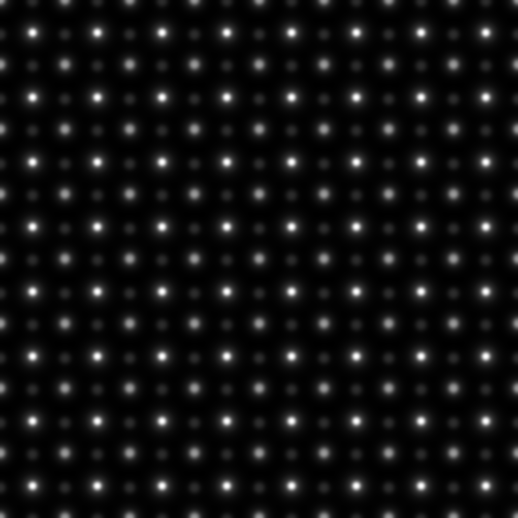
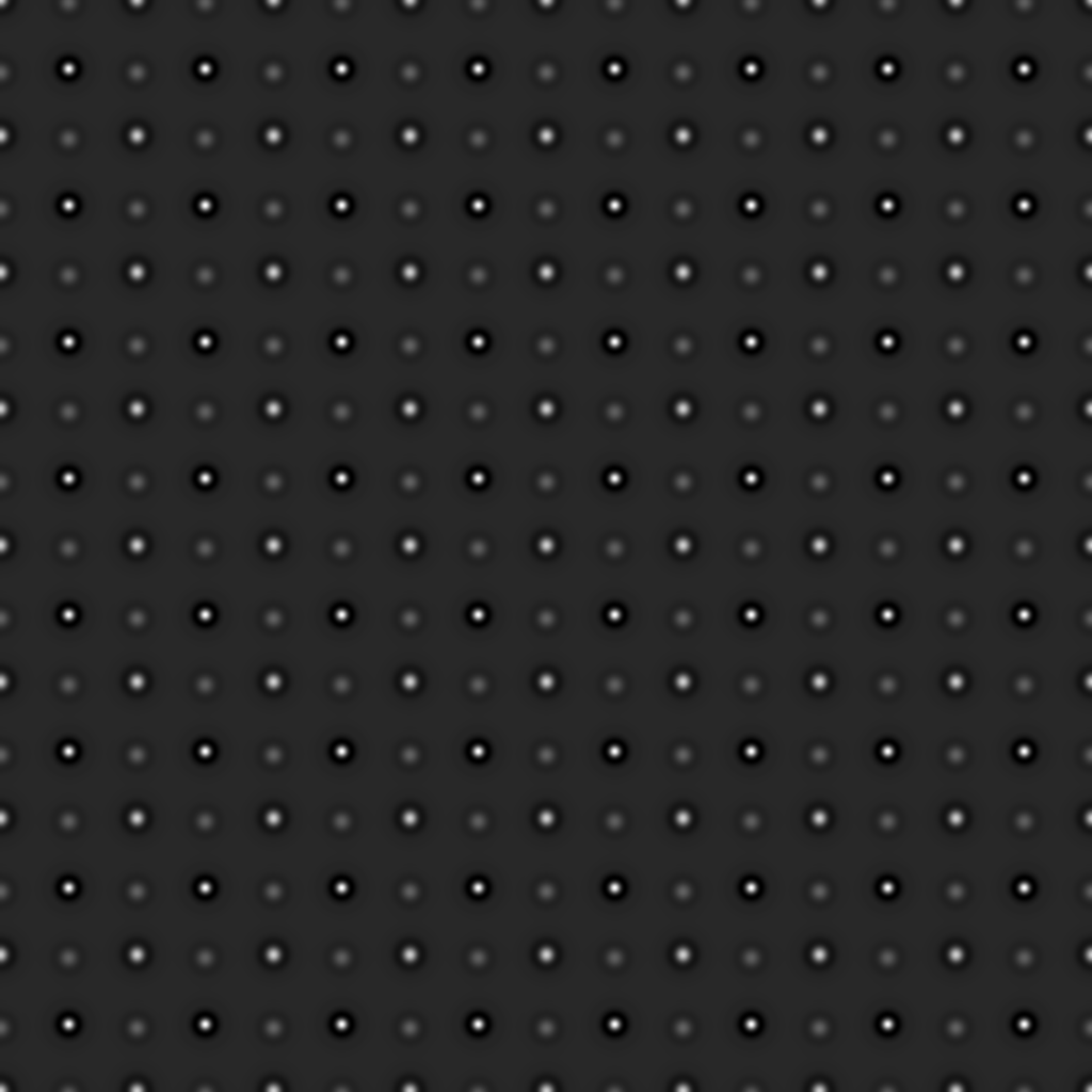
Figure 1: Phase and amplitude of the simulated exit wave. The images depict an area of $3.2\times 3.2$ nm² and are sampled with $1024\times 1024$ pixels.

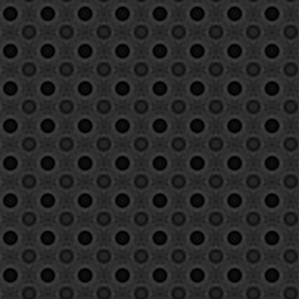
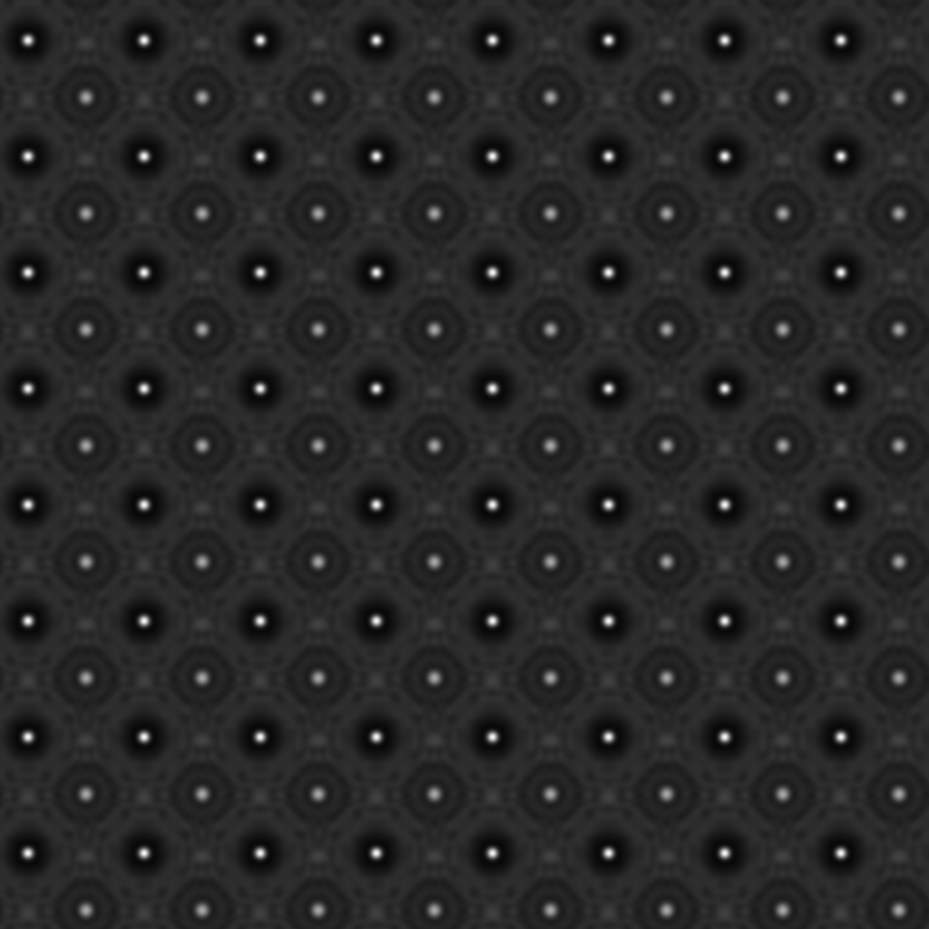
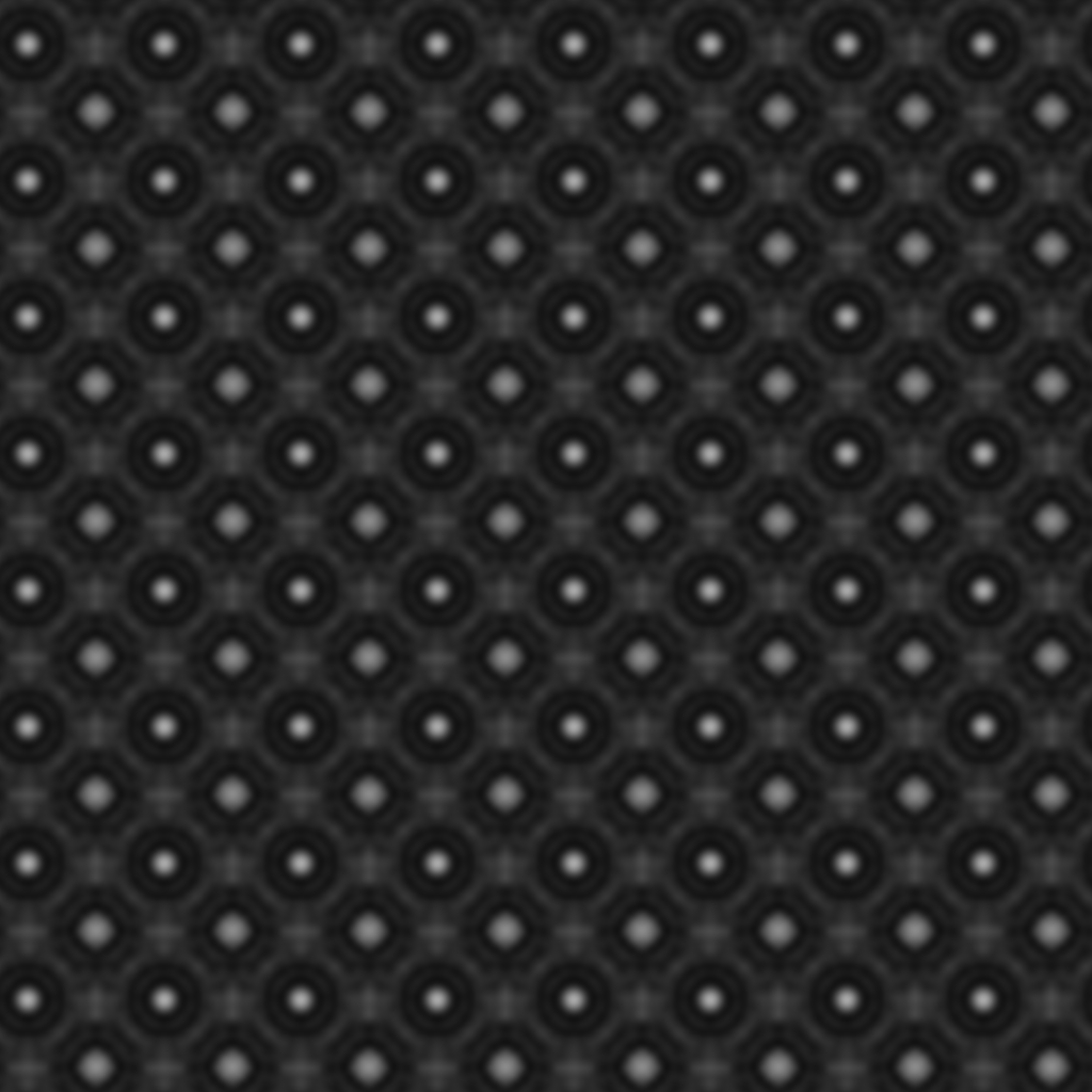
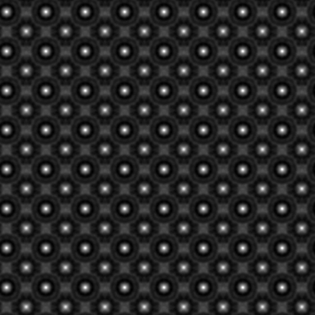
Figure 2: From left to right, top to bottom: Images 6 to 9 of the simulated focus series with focus values of $-1$, $0.5$, $2$, and $3.5$ nanometer respectively. The image series was simulated with a spherical aberration coefficient of $C_{s}=-70$nm and an objective aperture of $\alpha_{\text{max}}=125$mrad. The electron wavelength is $0.00196875$nm, which corresponds to an accelerating voltage of $300$kV. The images depict an area of $3.2\times 3.2$ nm² and are sampled with $1024\times 1024$ pixels.

For the practical minimization of the functional $E_{\alpha}$ it is important to note two sources of non-uniqueness for a minimizer $(\Psi,t)$ in the case $\Psi_{M}=0$. In this case, multiplying the exit wave with a global phase factor $e^{\text{i}c}$ for a $c\in\mathbb{R}$ does not change the energy, i.e.

$$E_{\alpha}[\Psi e^{ic},t]=E_{\alpha}[\Psi,t]$$ (11)

holds for all $c\in\mathbb{R}$. However, in practice we observed that the lowest frequency of $\Psi$ remained approximately equal to $1$ during the entire minimization, which indicates that Equation 11 does not affect a derivative based minimization method such as the conjugate gradient method. Another source of non-uniqueness is the fact that a ”global” modulation of the exit wave and all images does not change the energy, i.e.

$$E_{\alpha}[\Psi\mu_{s},t_{s}]=E_{\alpha}[\Psi,t]$$

holds for all $s\in\mathbb{R}^{2}$, where $t_{s}=(t_{1}+s,\,t_{2}+s,\,...,\,t_{N}+s)\in(\mathbb{R}^{2})^{N}$. This ambiguity can easily be solved by choosing the first image as a reference and keeping $t_{1}=0$ fixed.

The minimization of our objective functional $E_{\alpha}$ was performed with the regularization coefficient set to $\alpha:=10^{-5}$. No a-priori estimate of the exit wave is used for the minimization and thus $\Psi_{M}$ is set to zero. As the initial guess for the exit wave we used a constant wave equal to the square root of the mean image intensities. The initial guess for the translations was obtained by registering successive images in the simulated image series with the cross-correlation. This only gives a very rough estimate of the true image shifts, but is sufficiently accurate as an initial guess for the minimization. After $183$ steps of the nonlinear conjugate gradient method the minimization stops, where we used

$$E_{\alpha}[\Psi_{k-1},t_{k-1}]-E_{\alpha}[\Psi_{k},t_{k}]<\varepsilon:=10^{-10}$$

as the stopping criterion. Here $(\Psi_{k},t_{k})$ is the estimate of the exit wave and the translation after the $k$-th step.

In Figure 3 it can be seen that the data term is minimized successfully, while the value of the regularizer essentially stays constant. Furthermore, Figure 4 shows that the minimization also yielded good approximations to the correct translations and Figure 5 shows that the reconstructed exit wave is an approximation to the central section of the exit wave that was used for the input data simulation. Neither the phase and the amplitude of the reconstructed exit wave nor simulated TEM images based on the reconstructed exit wave are shown here, since they are visually identical to the images in Figures 1 and 2. The pixel value ranges are $[0.0693,1.815]$ (reconstructed), $[0.0741,1.824]$ (correct) of the phase and $[0.8747,1.637]$ (reconstructed), $[0.8746,1.645]$ (correct) of the amplitude of the exit wave.

Figure 3: Logarithmic plot of the energy and its components on the $y$-axis and the number of iterations of the nonlinear conjugate gradient method on the $x$-axis.

Figure 4: Distance of the estimated translation to the correct translation with respect to the supremum norm (orange graph) and the euclidean norm (blue graph). The number of iterations of the nonlinear conjugate gradient method is given on the $x$-axis and the distance in pixels is given on the $y$-axis.

Figure 5: Distance of the estimated exit wave in real space coordinates to the central section of the exit wave that was used for the input data simulation with respect to the supremum norm (orange graph) and the euclidean norm (blue graph, not normalized by the number of pixels).

6 Conclusions and outlook

We have shown that the transmission cross-coefficient $T_{Z}$ satisfies the factorization property, which, together with the concept of weighted cross-correlations, formed the basis for all further results. We then proposed a novel functional for joint exit wave reconstruction and image registration and derived expressions for the first and higher order Gâteaux differentials. We have shown that our objective functional is not convex with respect to the exit wave except in a trivial case, which also applies to the MAL functional. Using the direct method, we continued to show that minimizers of the Tikhonov-regularized version of our objective functional exist. Finally, the applicability of our approach was demonstrated with a numerical experiment on simulated input data.

In its current form, the problem of exit wave reconstruction using our objective functional is clearly not well-posed, since a minimizer is not unique. Therefore, it would be interesting to investigate additional assumptions or restrictions on our objective functional that are sufficient to ensure a unique minimizer. Similarly, it is not clear if the reconstructed exit wave depends continuously on the input data.

In practice, the focus step size between successive images in a focus series is very well known, but the available estimate of the actual focus value from the microscope settings is quite inaccurate. Therefore, an extension of our model that includes the base focus value as an unknown appears to be especially useful for the application of our method to real experimental data obtained with a TEM.

Extending the registration method to a piecewise rigid registration would allow for a reconstruction of the exit wave even if the specimen consists of multiple parts that move in different directions.

From a theoretical point of view it would be desirable to have a more complete result regarding the coercivity, since we have only shown that a particular variant of our objective functional is not coercive.

Appendix A Weighted cross-correlation

This section is a collection of various results regarding a generalization of the ordinary cross-correlation. The proofs are largely a direct generalization of the corresponding proofs for the ordinary cross-correlation.

Definition A.1.

Let $f,g:\mathbb{R}^{d}\rightarrow\mathbb{C}$ and $w:\mathbb{R}^{d}\times\mathbb{R}^{d}\rightarrow\mathbb{C}$. The weighted cross-correlation $f\star_{w}g$ is defined as

$$\big{(}f\star_{w}g\big{)}(x):=\int_{\mathbb{R}^{d}}f^{*}(y)g(x+y)w(x+y,y)\,\mathrm{d}y$$

for all $x\in\mathbb{R}^{d}$ such that the integral is well defined and finite.

This definition is extended to functions $f:M_{1}\rightarrow\mathbb{C}$ and $g:M_{2}\rightarrow\mathbb{C}$ for subsets $M_{1},M_{2}\subseteq\mathbb{R}^{d}$ by setting $f(x):=0$ for $x\in\mathbb{R}^{d}\backslash M_{1}$ and $g(x):=0$ for $x\in\mathbb{R}^{d}\backslash M_{2}$. It is similarly extended to weight functions $w:M_{3}\times M_{4}\rightarrow\mathbb{C}$ for subsets $M_{3},M_{4}\subseteq\mathbb{R}^{d}$.

Two vector spaces of weight functions are particularly useful here, so they are given a special notation. For $U\subseteq\mathbb{R}^{d}$, the space of measurable and bounded weight functions is defined as

$$W(U):=\{w:U\times U\rightarrow\mathbb{C}\mid w\text{ measurable and bounded}\}.$$

The subspace $W^{+}(U)$ of $W(U)$, where every function can be approximated by a particular kind of sequence of factorizable functions, is defined as

$$W^{+}(U):=\Big{\{}w\in W(U)\;\Big{|}\;\forall\,N\in\mathbb{N}\;\forall\,j\in\{1,\ldots,N\}\;\exists\,w_{N}\in W(U)$$

$$\;\;\exists\,v_{j,N}:U\rightarrow\mathbb{C}\text{ measurable and bounded}:$$

$$\left.\lim_{N\rightarrow\infty}\left|\left|w-w_{N}\right|\right|_{\infty}=0\;\wedge\;w_{N}(x,y)=\sum\nolimits_{j=1}^{N}v_{j,N}(x)v_{j,N}^{*}(y)\right\}.$$

In the following, we will consider the weighted cross-correlation for Lebesgue functions. This makes sense for $f$ and $g$, as the integration in Definition A.1 is carried out over the entire domain of $f$ and $g$. However, it does not make sense to consider the weight as a Lebesgue function, as the integration is only carried out over a subset of the weight’s domain of measure zero (namely, the diagonals $\{(x+y,y)\mid y\in\mathbb{R}^{d}\}$). It should be possible to extend the definition to weights $\widetilde{w}\in L^{\infty}(U\times U,\mathbb{C})$ by treating $f\star_{\widetilde{w}}g$ itself as a Lebesgue function, but this approach does not have any benefits for the theory developed in Sections 2, 3 and 4 and therefore is not pursued. Nevertheless, we occasionally identify a weight $w\in W(U)$ with the equivalence class $[w]\in L^{\infty}(U\times U,\mathbb{C})$ in order to be able to apply Hölder’s inequality.

Lemma A.2.

If $f,g\in L^{2}(\mathbb{R}^{d},\mathbb{C})$ and $w\in W(\mathbb{R}^{d})$, then $(f\star_{w}g)(x)\in\mathbb{C}$ for all $x\in\mathbb{R}^{d}$ and $\left|\left|f\star_{w}g\right|\right|_{\infty}\leq\left|\left|w\right|\right|_{\infty}\left|\left|f\right|\right|_{L^{2}}\left|\left|g\right|\right|_{L^{2}}$.

Proof.

This follows from the Cauchy-Schwarz inequality.∎

Lemma A.3.

Let $p\in[1,\infty)$. If $f\in L^{1}(\mathbb{R}^{d},\mathbb{C})$, $g\in L^{p}(\mathbb{R}^{d},\mathbb{C})$ and $w\in W(\mathbb{R}^{d})$, then $f\star_{w}g\in L^{p}(\mathbb{R}^{d},\mathbb{C})$ and $\left|\left|f\star_{w}g\right|\right|_{L^{p}}\leq\left|\left|w\right|\right|_{\infty}\left|\left|f\right|\right|_{L^{1}}\left|\left|g\right|\right|_{L^{p}}$.

Proof.

This can be shown with a straightforward application of Minkowski’s integral inequality.∎

An immediate consequence of Lemma A.3 is that the space $L^{1}(\mathbb{R}^{d},\mathbb{C})$ is closed under weighted cross-correlation. If the support of the weight is bounded, then the same is true for every $L^{p}$-space with $p\in[1,\infty)$.

Corollary A.4.

If $p\in[1,\infty)$ and $w\in W(U)$ for a bounded subset $U\subseteq\mathbb{R}^{d}$, then $f\star_{w}g\in L^{p}(\mathbb{R}^{d},\mathbb{C})$ for all $f,g\in L^{p}(\mathbb{R}^{d},\mathbb{C})$.

Proof.

Since the support of $w$ is bounded, there is an $r>0$ such that

$$\mathrm{supp}(w)\subseteq B_{r}(0)\subseteq\mathbb{R}^{d}\times\mathbb{R}^{d}.$$

Let $A:=B_{r}(0)\subseteq\mathbb{R}^{d}$. Then $w(x,y)=w(x,y)\chi_{A}(x)\chi_{A}^{*}(y)$ for all $x,y\in\mathbb{R}^{d}$ and it follows that

$$f\star_{w}g=(f\chi_{A})\star_{w}(g\chi_{A}).$$

Since $f\chi_{A}\in L^{p}(\mathbb{R}^{d},\mathbb{C})$ has bounded support, we get $f\chi_{A}\in L^{1}(\mathbb{R}^{d},\mathbb{C})$ from Hölder’s inequality and consequently $f\star_{w}g\in L^{p}(\mathbb{R}^{d},\mathbb{C})$ by the previous lemma. ∎

The next lemma lists two symmetry properties that are useful to simplify calculations with weighted cross-correlations.

Lemma A.5.

Let $f,g\in L^{2}(\mathbb{R}^{d},\mathbb{C})$ and $w\in W(U)$ for a bounded subset $U\subseteq\mathbb{R}^{d}$ with $w^{*}(x,y)=w(y,x)$ for all $x,y\in\mathbb{R}^{d}$. Then

1. $\big{(}f\star_{w}g\big{)}(x)=\big{(}g\star_{w}f\big{)}^{*}(-x)$ for all $x\in\mathbb{R}^{d}$.

2. $(h,f\star_{w}g)_{L^{2}}=(g\star_{w}f,h)_{L^{2}}$ for all $h\in L^{2}(\mathbb{R}^{d},\mathbb{C})$ with $h(x)=h^{*}(-x)$ for all $x\in\mathbb{R}^{d}$.

Proof.

Both statements follow directly from the definition of the weighted cross-correlation. ∎

The first symmetry property can be used to derive the following results on the weighted autocorrelation of $L^{2}$-functions.

Lemma A.6.

Let $f\in L^{2}(\mathbb{R}^{d},\mathbb{C})$ and $w\in W^{+}(U)$ for a bounded subset $U\subseteq\mathbb{R}^{d}$ with $w^{*}(x,y)=w(y,x)$ for all $x,y\in\mathbb{R}^{d}$. Then $\mathcal{F}^{-1}(f\star_{w}f)$ is real-valued and nonnegative.

Proof.

By the first symmetry property of Lemma A.5, we have

$$\big{(}f\star_{w}f\big{)}(x)=\big{(}f\star_{w}f\big{)}^{*}(-x)$$

for all $x\in\mathbb{R}^{d}$, which implies that $\mathcal{F}^{-1}(f\star_{w}f)$ is real-valued.

Let $(w_{N})_{N\in\mathbb{N}}\in W(U)^{\mathbb{N}}$ and $v_{j,N}:U\rightarrow\mathbb{C}$ measurable and bounded such that $\lim_{N\rightarrow\infty}\left|\left|w-w_{N}\right|\right|_{\infty}=0$ and $w_{N}(x,y)=\sum_{j=1}^{N}v_{j,N}(x)v_{j,N}^{*}(y)$ for all $N\in\mathbb{N}$. By the same reasoning as in Corollary A.4 it is possible to assume without loss of generality that $\operatorname{supp}(f)$ is bounded. This implies $f\in L^{1}(\mathbb{R}^{d},\mathbb{C})$ and shows that $f\star_{w_{N}}f\in L^{1}(\mathbb{R}^{d},\mathbb{C})$ for all $N\in\mathbb{N}$ by Lemma A.3. Therefore, $\mathcal{F}^{-1}(f\star_{w_{N}}f)$ is continuous and the inequality

$$\mathcal{F}^{-1}(f\star_{w_{N}}f)=\sum_{j=1}^{N}\left|\mathcal{F}^{-1}(fv_{j,N})\right|^{2}\geq 0$$ (12)

holds for all $N\in\mathbb{N}$ by the linearity of the Fourier transform and the convolution theorem. Since the Fourier transform is unitary, it follows that

$$\left|\left|\mathcal{F}^{-1}(f\star_{w}f)-\mathcal{F}^{-1}(f\star_{w_{N}}f)\right|\right|_{L^{2}} =\left|\left|f\star_{(w-w_{N})}f\right|\right|_{L^{2}}$$

$$\leq\left|\left|w-w_{N}\right|\right|_{\infty}\left|\left|f\star f\right|\right|_{L^{2}}\underset{N\rightarrow\infty}{\longrightarrow}0,$$

where $\left|\left|f\star f\right|\right|_{L^{2}}<\infty$ since $\operatorname{supp}(f)$ is bounded. Thus $\mathcal{F}^{-1}(f\star_{w_{N}}f)\rightarrow\mathcal{F}^{-1}(f\star_{w}f)$ in $L^{2}$ and consequently there exists a subsequence of $\big{(}\mathcal{F}^{-1}(f\star_{w_{N}}f)\big{)}_{N\in\mathbb{N}}$ converging pointwise to $\mathcal{F}^{-1}(f\star_{w}f)$. But all elements of $\big{(}\mathcal{F}^{-1}(f\star_{w_{N}}f)\big{)}_{N\in\mathbb{N}}$ are nonnegative by Equation 12, which shows that $\mathcal{F}^{-1}(f\star_{w}f)$ is nonnegative as well.∎

Corollary A.7.

Let $U\subseteq\mathbb{R}^{d}$ be bounded and $w\in W^{+}(U)$ such that $w^{*}(x,y)=w(y,x)$ for all $x,y\in\mathbb{R}^{d}$. Then the functional

$$F:L^{2}(\mathbb{R}^{d},\mathbb{C})\rightarrow\mathbb{R},\quad f\mapsto\left|\left|f\star_{w}f\right|\right|_{L^{2}}^{2}$$

is Fréchet differentiable, continuous and convex.

Proof.

Analogously to Corollary 3.3, we get that

$$F^{\prime}[f]:L^{2}(\mathbb{R}^{d},\mathbb{C})\rightarrow\mathbb{R},\quad g\mapsto 2\mathrm{Re}\big{(}(f\star_{w}f,f\star_{w}g+g\star_{w}f)_{L^{2}}\big{)}$$

is the first order Gâteaux differential of $F$ at $f\in L^{2}(\mathbb{R}^{d},\mathbb{C})$ in the direction $g\in L^{2}(\mathbb{R}^{d},\mathbb{C})$ and

$$\left|F^{\prime}[f](g)\right| \leq 2\left|\left|f\star_{w}f\right|\right|_{L^{2}}\left|\left|f\star_{w}g+g\star_{w}f\right|\right|_{L^{2}}\leq 4\left|\left|f\star_{w}f\right|\right|_{L^{2}}\left|\left|f\star_{w}g\right|\right|_{L^{2}}$$

$$\leq 4\left|\left|f\star_{w}f\right|\right|_{L^{2}}\left|\left|w\right|\right|_{\infty}\left|\left|f\right|\right|_{L^{1}}\left|\left|g\right|\right|_{L^{2}}$$

holds for all $g\in L^{2}(U,\mathbb{C})$ by Lemma A.5 (i) and Lemma A.3. Therefore, $F^{\prime}[f]$ is a bounded linear operator that additionally satisfies

$$\lim_{g\rightarrow 0}\frac{\left|F[f+g]-F[f]-F^{\prime}[f](g)\right|}{\left|\left|g\right|\right|_{L^{2}}}=0,$$

which shows that $F$ is Fréchet differentiable and particularly continuous.

Analogously to Corollary 3.3, the second order Gâteaux differential of $F$ at a position $f\in L^{2}(U,\mathbb{C})$ in the direction $g\in L^{2}(U,\mathbb{C})$ is

$$\langle F^{\prime\prime}[f],g\rangle =\left|\left|f\star_{w}g+g\star_{w}f\right|\right|_{L^{2}}^{2}+2\mathrm{Re}\big{(}(f\star_{w}f,g\star_{w}g)_{L^{2}}\big{)}$$

$$=\left|\left|f\star_{w}g+g\star_{w}f\right|\right|_{L^{2}}^{2}+2\mathrm{Re}\big{(}(\mathcal{F}^{-1}(f\star_{w}f),\mathcal{F}^{-1}(g\star_{w}g))_{L^{2}}\big{)}.$$

By Lemma A.6 we have $\langle F^{\prime\prime}[f],g\rangle\geq 0$ for all $f,g\in L^{2}(U,\mathbb{C})$, which implies that $F$ is convex.∎

Similar to the ordinary cross-correlation, the weighted cross-correlation of $L^{p}$- and $L^{q}$-functions is continuous for suitable weight functions. Note that the constant weight function $w(x,y)=1$ for all $x,y\in\mathbb{R}^{d}$ satisfies all of the conditions in the following Lemma, which therefore is a direct generalization of the corresponding statement for the ordinary cross-correlation.

Lemma A.8.

Let $U\subseteq\mathbb{R}^{d}$ be an open set such that the measure of its boundary $\partial U$ is zero and $p,q\in(1,\infty)$ with $\frac{1}{p}+\frac{1}{q}=1$. Choose $f\in L^{p}(U,\mathbb{C})$, $g\in L^{q}(U,\mathbb{C})$ and $w\in W(U)$. If $w$ is continuous on $U\times U$, then $f\star_{w}g\in C(\mathbb{R}^{d},\mathbb{C})$.

Proof.

Fix an arbitrary $x\in\mathbb{R}^{d}$ and let $\varepsilon>0$. We show that $f\star_{w}g$ is continuous at $x$. Since $C_{c}(\mathbb{R}^{d},\mathbb{C})$ is dense in $L^{q}(\mathbb{R}^{d},\mathbb{C})$, there is a function $v\in C_{c}(\mathbb{R}^{d},\mathbb{C})$ with $\left|\left|g-v\right|\right|_{L^{q}}<\varepsilon$. Define

$$G_{z}:\mathbb{R}^{d}\rightarrow\mathbb{C},\quad y\mapsto g(z+y)w(z+y,y),$$

$$V_{z}:\mathbb{R}^{d}\rightarrow\mathbb{C},\quad y\mapsto v(z+y)w(z+y,y)$$

for all $z\in\mathbb{R}^{d}$. By the Hölder and Minkowski inequalities,

$$\left|\big{(}f\star_{w}g\big{)}(x+h)-\big{(}f\star_{w}g\big{)}(x)\right|$$

$$\leq\; \int\left|f^{*}(y)g(x+h+y)w(x+h+y,y)-f^{*}(y)g(x+y)w(x+y,y)\right|\,\mathrm{d}y$$

$$\leq\; \left|\left|f\right|\right|_{L^{p}}\left|\left|G_{x+h}-G_{x}\right|\right|_{L^{q}}$$

$$\leq\; \left|\left|f\right|\right|_{L^{p}}\big{(}\left|\left|G_{x+h}-V_{x+h}\right|\right|_{L^{q}}+\left|\left|V_{x+h}-V_{x}\right|\right|_{L^{q}}+\left|\left|V_{x}-G_{x}\right|\right|_{L^{q}}\big{)}$$

holds for all $h\in\mathbb{R}^{d}$. An upper bound for the first and third summand is given by

$$\left|\left|G_{z}-V_{z}\right|\right|_{L^{q}}\leq\left|\left|g-v\right|\right|_{L^{q}}\left|\left|w\right|\right|_{\infty}<\varepsilon\left|\left|w\right|\right|_{\infty} \forall\,z\in\mathbb{R}^{d}$$ .

By the continuity of $v$ and the continuity of $w$ on $U\times U$, we have

$$\lim_{h\rightarrow 0}V_{x+h}(y) =\lim_{h\rightarrow 0}v(x+h+y)w(x+h+y,y)$$

$$=\begin{cases}v(x+y)w(x+y,y),&\text{if $y\in U\;\;\wedge\;\;x+y\in U$},\\ 0,&\text{if $y\in U\;\;\wedge\;\;x+y\in\overline{U}^{c}$},\\ 0,&\text{if $y\in U^{c}$},\end{cases}$$

$$=\begin{cases}V_{x}(y),&y\in U\;\;\wedge\;\;x+y\in U,\\ V_{x}(y),&y\in U\;\;\wedge\;\;x+y\in\overline{U}^{c},\\ V_{x}(y),&y\in U^{c}.\end{cases}$$

This implies $\lim_{h\rightarrow 0}V_{x+h}(y)=V_{x}(y)$ for almost all $y\in\mathbb{R}^{d}$, since $\partial U$ has zero measure and thus also the set $\{y\in U\mid x+y\in\partial U\}$. Furthermore, since $\left|V_{x+h}(y)\right|\leq\left|\left|w\right|\right|_{\infty}\left|\left|v\right|\right|_{\infty}<\infty$ for all $y\in\mathbb{R}^{d}$ and

$$\operatorname{supp}(V_{x+h})\subseteq\overline{B_{1}\big{(}\operatorname{supp}(v)-x\big{)}}=:D\qquad\qquad\forall\,h\in B_{1}(0),$$

it follows that $\left|\left|w\right|\right|_{\infty}\left|\left|v\right|\right|_{\infty}\chi_{D}$ is an integrable function that dominates $V_{x+h}$ for all $h\in B_{1}(0)$. Now the dominated convergence theorem implies

$$\lim_{h\rightarrow 0}\left|\left|V_{x+h}-V_{x}\right|\right|_{L^{q}}=0$$

and we conclude $\lim\limits_{h\rightarrow 0}\left|\big{(}f\star_{w}g\big{)}(x+h)-\big{(}f\star_{w}g\big{)}(x)\right|=0$. ∎

An application of the continuity of the weighted cross-correlation is the following characterization of $L^{2}$-functions, whose weighted autocorrelation is zero.

Lemma A.9.

Let $U\subseteq\mathbb{R}^{d}$ be an open set such that the measure of its boundary $\partial U$ is zero. Choose $f\in L^{2}(U,\mathbb{C})$ and a continuous weight $w\in W(U)$. If there is a $c>0$ with $w(y,y)\geq c$ for almost all $y\in U$, then

$$\left|\left|f\star_{w}f\right|\right|_{L^{2}}=0\qquad\Longleftrightarrow\qquad\left|\left|f\right|\right|_{L^{2}}=0.$$

Proof.

”$\Leftarrow$”: $\left|\left|f\right|\right|_{L^{2}}=0$ implies $f=0$ almost everywhere and thus $\left|\left|f\star_{w}f\right|\right|_{L^{2}}=0$. ”$\Rightarrow$”: If $\left|\left|f\star_{w}f\right|\right|_{L^{2}}=0$, then $f\star_{w}f=0$ almost everywhere. However, the function $f\star_{w}f$ is continuous by Lemma A.8, which implies $f\star_{w}f=0$. In particular,

$$0=\big{(}f\star_{w}f\big{)}(0)=\int_{U}\left|f(y)\right|^{2}w(y,y)\,\mathrm{d}y\geq c\left|\left|f\right|\right|_{L^{2}}^{2}\geq 0$$

and thus $\left|\left|f\right|\right|_{L^{2}}=0$.∎

Appendix B Low-pass filter approximation

It is easy to see that the functional $f\mapsto\left|\left|f\star f\right|\right|_{L^{2}}$ with $f\in L^{2}(\mathbb{R}^{d},\mathbb{C})$ is not coercive. If we define

$$g_{\delta}:\mathbb{R}^{d}\rightarrow\mathbb{R},\quad x\mapsto\begin{cases}\prod_{i=1}^{d}\frac{1}{\sqrt{x_{i}}},&\text{if }1\leq x_{i}\leq\delta\;\,\forall\,i\in\{1,\ldots,d\},\\ 0,&\text{otherwise}\end{cases}$$

for all $\delta>1$, then $\lim_{\delta\rightarrow\infty}\left|\left|g_{\delta}\right|\right|_{L^{2}}=\infty$ and $\lim_{\delta\rightarrow\infty}\left|\left|g_{\delta}^{2}\right|\right|_{L^{2}}=1$. Therefore, it follows that

$$\lim_{\delta\rightarrow\infty}\left|\left|f_{\delta}\right|\right|_{L^{2}}=\infty\qquad\text{and}\qquad\lim_{\delta\rightarrow\infty}\left|\left|f_{\delta}\star f_{\delta}\right|\right|_{L^{2}}=\lim_{\delta\rightarrow\infty}\left|\left|(\mathcal{F}^{-1}f_{\delta})^{2}\right|\right|_{L^{2}}=1$$

for $f_{\delta}=\mathcal{F}g_{\delta}$.

The purpose of this section is to generalize this result to

$$f\mapsto\left|\left|f\star f\right|\right|_{L^{2}},\qquad f\in L^{2}(U,\mathbb{C})$$

for any open set $U\subseteq\mathbb{R}^{d}$ with non-empty interior. The central tool to this end is Lemma B.1, which provides a method to estimate how well a function $g:\mathbb{R}\rightarrow\mathbb{R}$ is approximated by $g*\operatorname{sinc}$. Here, $\operatorname{sinc}$ is the normalized cardinal sine function defined as

$$\operatorname{sinc}(x)=\begin{cases}\frac{\sin(\pi x)}{\pi x},&\text{if $x\neq 0$,}\\ 1,&\text{if $x=0$.}\end{cases}$$

We have $\mathcal{F}(\operatorname{sinc})=\chi_{[-\frac{1}{2},\frac{1}{2}]}$ so that the convolution of $g$ with $\operatorname{sinc}$ corresponds to applying an ideal low-pass filter with cutoff frequency $\frac{1}{2}$ to $g$.

In order to compute bounds for real-valued functions, we make use of interval arithmetic. The sum and the difference of two intervals $I_{1}:=[a,b]$ and $I_{2}:=[c,d]$ are

$$I_{1}+I_{2} :=\{x+y\mid x\in I_{1},\,y\in I_{2}\}=[a+c,b+d],$$

$$I_{1}-I_{2} :=\{x-y\mid x\in I_{1},\,y\in I_{2}\}=[a-d,b-c]$$

for all $a,b,c,d\in\mathbb{R}$ with $a\leq b$ and $c\leq d$.

Lemma B.1.

Let $g:\mathbb{R}\rightarrow\mathbb{R}$ be monotonic, bounded and positive, $k\in L^{1}_{\textnormal{loc}}(\mathbb{R},\mathbb{R})$ and $N>0$. If there are constants $\alpha_{N},\beta_{N}>0$ such that

• $\left|\int_{I}k(y)\,\mathrm{d}y\right|\leq\alpha_{N}$ for all intervals $I\subseteq[-N,N]$,

• $\left|\int_{I}k(y)\,\mathrm{d}y\right|\leq\beta_{N}$ for all bounded intervals $I\subseteq\mathbb{R}\backslash[-N,N]$,

then

$$\big{(}g*k\big{)}(x)\in\delta_{N}g(x-N)+\left|g(x+N)-g(x-N)\right|[-\alpha_{N},\alpha_{N}]+4\left|\left|g\right|\right|_{\infty}[-\beta_{N},\beta_{N}],$$

where $\delta_{N}=\int_{[-N,N]}k(y)\,\mathrm{d}y$, holds for all $x\in\mathbb{R}$.

Proof.

Let $x\in\mathbb{R}$ and split the integral into three parts,

$$\big{(}g\ast k\big{)}(x)=\int_{-N}^{N}g(x-y)k(y)\,\mathrm{d}y+\int_{N}^{\infty}g(x-y)k(y)\,\mathrm{d}y+\int_{-\infty}^{-N}g(x-y)k(y)\,\mathrm{d}y.$$

By the second mean value theorem of integral calculus [10] there exists a $B\in[-N,N]$ with

$$\int_{-N}^{N}g(x-y)k(y)\,\mathrm{d}y =g(x+N)\int_{-N}^{B}k(y)\,\mathrm{d}y+g(x-N)\int_{B}^{N}k(y)\,\mathrm{d}y$$

$$=g(x+N)\int_{-N}^{B}k(y)\,\mathrm{d}y+g(x-N)\left(\delta_{N}-\int_{-N}^{B}k(y)\,\mathrm{d}y\right)$$

$$=\big{(}g(x+N)-g(x-N)\big{)}\int_{-N}^{B}k(y)\,\mathrm{d}y+\delta_{N}g(x-N)$$

$$\in\left|g(x+N)-g(x-N)\right|[-\alpha_{N},\alpha_{N}]+\delta_{N}g(x-N).$$

Bounds for the other two integrals can also be found using the second mean value theorem: for every $M>N$ there exists a $Q_{M}\in[N,M]$ with

$$\int_{N}^{\infty}g(x-y)k(y)\,\mathrm{d}y =\lim_{M\rightarrow\infty}\int_{N}^{M}g(x-y)k(y)\,\mathrm{d}y$$

$$=\lim_{M\rightarrow\infty}g(x-N)\int_{N}^{Q_{M}}k(y)\,\mathrm{d}y+g(x-M)\int_{Q_{M}}^{M}k(y)\,\mathrm{d}y$$

$$\in 2\left|\left|g\right|\right|_{\infty}[-\beta_{N},\beta_{N}]$$

and similarly for the third integral.∎

If $k=\operatorname{sinc}$ is chosen as the convolution kernel in the previous lemma, the constants $\alpha_{N}$ and $\beta_{N}$ as well as a bound on $\delta_{N}$ can be found as follows.

If $I=[c,d]\subset\mathbb{R}$ is a bounded interval, then

$$\int_{I}k(y)\,\mathrm{d}y=\frac{1}{\pi}\int_{\pi c}^{\pi d}\frac{\sin(y)}{y}\,\mathrm{d}y=\frac{1}{\pi}\big{(}\operatorname{Si}(\pi d)-\operatorname{Si}(\pi c)\big{)},$$

where $\operatorname{Si}$ is the sine integral defined as $\operatorname{Si}(x)=\int_{0}^{x}{\sin(y)}/{y}\,\mathrm{d}y$ for all $x\in\mathbb{R}$. It is well known that $\left|\operatorname{Si}(x)\right|\leq\operatorname{Si}(\pi)\leq 2$ for all $x\in\mathbb{R}$. Moreover, we have $\left|\operatorname{Si}(x)-\frac{\pi}{2}\right|\leq\frac{1}{x}$ for all $x>0$, which can be shown with the Laplace transform. Because of the point symmetry of the sine integral it follows that $\left|\operatorname{Si}(x)+\frac{\pi}{2}\right|\leq\frac{1}{-x}$ for all $x<0$.

Fix an arbitrary $N>0$. If $I=[c,d]\subseteq[-N,N]$, then

$$\left|\int_{I}k(y)\,\mathrm{d}y\right|=\frac{1}{\pi}\left|\operatorname{Si}(\pi d)-\operatorname{Si}(\pi c)\right|\leq\frac{1}{\pi}(2+2)=\frac{4}{\pi}=:\alpha_{N},$$

On the other hand, if we consider an interval $I=[c,d]\subseteq(N,\infty)$, then

$$\left|\int_{I}k(y)\,\mathrm{d}y\right| =\frac{1}{\pi}\left|\operatorname{Si}(\pi d)-\operatorname{Si}(\pi c)\right|=\frac{1}{\pi}\left|\left(\operatorname{Si}(\pi d)-\frac{\pi}{2}\right)-\left(\operatorname{Si}(\pi c)-\frac{\pi}{2}\right)\right|$$

$$\leq\frac{1}{\pi}\left(\frac{1}{\pi d}+\frac{1}{\pi c}\right)\leq\frac{2}{\pi^{2}N}=:\beta_{N}$$

and similarly $\left|\int_{I}f(y)\,\mathrm{d}y\right|\leq\frac{2}{\pi^{2}N}$ for $I=[c,d]\subseteq(-\infty,-N)$. The value of $\delta_{N}$ is bounded by

$$\left|\delta_{N}-1\right|=\left|\int_{[-N,N]}k(y)\,\mathrm{d}y-1\right|=\left|\frac{2}{\pi}\operatorname{Si}(\pi N)-1\right|\leq\frac{2}{\pi}\frac{1}{\pi N}=\frac{2}{\pi^{2}N}.$$

Lemma B.2.

The functional $f\mapsto\left|\left|f\star f\right|\right|_{L^{2}}$ with $f\in L^{2}(I,\mathbb{C})$ is not coercive for any interval $I\subseteq\mathbb{R}$.

Proof.

For $\delta>1$ let $g_{\delta}:\mathbb{R}\rightarrow\mathbb{R}$ with $g_{\delta}(x)=\frac{1}{\sqrt{x}}$ for all $x\in[1,\delta]$ and $g_{\delta}(x)=0$ for all $x\in\mathbb{R}\backslash[1,\delta]$. The function $g_{\delta}$ is neither monotonic nor positive, but it can be written as the difference of two monotonic, bounded and positive functions $g_{\delta,1}$ and $g_{\delta,2}$, e.g.

$$g_{\delta,1}(x)=\begin{cases}1,&\text{if }x<1,\\ 2,&\text{if }x\geq 1\end{cases}\qquad\text{and}\qquad g_{\delta,2}(x)=\begin{cases}1,&\text{if }x<1,\\ 2-\frac{1}{\sqrt{x}},&\text{if }1\leq x\leq\delta,\\ 2,&\text{if }x>\delta.\end{cases}$$

Applying Lemma B.1 to $g_{\delta,j}$ for $j\in\{1,2\}$ and using $\alpha_{n}$ and $\beta_{N}$ as derived above as well as the bound on $\delta_{N}$ yields bounds $\big{(}g_{\delta,j}*k\big{)}(x)\in[L_{\delta,j,N}(x),U_{\delta,j,N}(x)]$ for all $x\in\mathbb{R}$ and all $N>0$, where

$$L_{\delta,j,N}(x) :=g_{\delta,j}(x-N)\left(1-\frac{2}{\pi^{2}N}\right)-\left|g_{\delta,j}(x+N)-g_{\delta,j}(x-N)\right|\frac{4}{\pi}-\frac{16}{\pi^{2}N},$$

$$U_{\delta,j,N}(x) :=g_{\delta,j}(x-N)\left(1+\frac{2}{\pi^{2}N}\right)+\left|g_{\delta,j}(x+N)-g_{\delta,j}(x-N)\right|\frac{4}{\pi}+\frac{16}{\pi^{2}N}.$$

Therefore, $g_{\delta}*k$ is bounded by

$$\big{(}g_{\delta}*k\big{)}(x) =\big{(}g_{\delta,1}*k\big{)}(x)-\big{(}g_{\delta,2}*k\big{)}(x)$$

$$\in[L_{\delta,1,N}(x)-U_{\delta,2,N}(x),U_{\delta,1,N}(x)-L_{\delta,2,N}(x)]$$

for all $x\in\mathbb{R}$ and all $N>0$. In particular, choosing $x=2N$ yields the lower bounds

$$\big{(}g_{\delta}*k\big{)}(2N)\geq\begin{cases}\left(1-\frac{12-4\sqrt{3}}{3\pi}\right)\frac{1}{\sqrt{N}}-\frac{40}{\pi^{2}}\frac{1}{N}+\frac{2}{\pi^{2}}\frac{1}{N\sqrt{N}},&\text{if }N\in\left[1,\frac{\delta}{3}\right],\\ \left(1-\frac{4}{\pi}\right)\frac{1}{\sqrt{N}}-\frac{40}{\pi^{2}}\frac{1}{N}+\frac{2}{\pi^{2}}\frac{1}{N\sqrt{N}},&\text{if }N\in\left(\frac{\delta}{3},\delta\right],\\ -\frac{40}{\pi^{2}N},&\text{if }N\in\left(\delta,\infty\right)\end{cases}$$

and the upper bounds

$$\big{(}g_{\delta}*k\big{)}(2N)\leq\begin{cases}\left(1+\frac{12-4\sqrt{3}}{3\pi}\right)\frac{1}{\sqrt{N}}+\frac{40}{\pi^{2}}\frac{1}{N}-\frac{2}{\pi^{2}}\frac{1}{N\sqrt{N}},&\text{if }N\in\left[1,\frac{\delta}{3}\right],\\ \left(1+\frac{4}{\pi}\right)\frac{1}{\sqrt{N}}+\frac{40}{\pi^{2}}\frac{1}{N}-\frac{2}{\pi^{2}}\frac{1}{N\sqrt{N}},&\text{if }N\in\left(\frac{\delta}{3},\delta\right],\\ \frac{40}{\pi^{2}N},&\text{if }N\in\left(\delta,\infty\right)\end{cases}$$

for all $N>1$. A bound on $\big{(}g_{\delta}*k\big{)}(x)$ for negative values of $x$ can be found similarly by choosing $x=-N$, which yields $\big{(}g_{\delta}*k\big{)}(-N)\in\left[\frac{-36}{\pi^{2}N},\frac{36}{\pi^{2}N}\right]$ for all $N>0$. Furthermore, $g_{\delta}*k$ is uniformly bounded by

$$\left|\left|g_{\delta}*k\right|\right|_{\infty}\leq\left|\left|g_{\delta}\right|\right|_{L^{4}}\left|\left|k\right|\right|_{L^{4/3}}\leq\left|\left|g_{\infty}\right|\right|_{L^{4}}\left|\left|k\right|\right|_{L^{4/3}}<\infty$$

for all $\delta>1$ by Hölder’s inequality. Using these bounds and the fact that the coefficient $1-\frac{12-4\sqrt{3}}{3\pi}$ of $\frac{1}{\sqrt{N}}$ in the lower bound of $\big{(}g_{\delta}*k\big{)}(2N)$ is positive, it follows that

$$\lim_{\delta\rightarrow\infty}\left|\left|g_{\delta}*k\right|\right|_{L^{2}}=\infty\qquad\text{and}\qquad\lim_{\delta\rightarrow\infty}\left|\left|(g_{\delta}*k)^{2}\right|\right|_{L^{2}}<\infty.$$

Without loss of generality we assume that $I=\left[-\frac{1}{2},\frac{1}{2}\right]$. If $f_{\delta}=(\mathcal{F}g_{\delta})\chi_{[-\frac{1}{2},\frac{1}{2}]}$ for all $\delta>1$, then $f_{\delta}\in L^{2}\left(\left[-\frac{1}{2},\frac{1}{2}\right],\mathbb{C}\right)$ and

$$\lim_{\delta\rightarrow\infty}\left|\left|f_{\delta}\right|\right|_{L^{2}} =\lim_{\delta\rightarrow\infty}\left|\left|\mathcal{F}^{-1}f_{\delta}\right|\right|_{L^{2}}=\lim_{\delta\rightarrow\infty}\left|\left|g_{\delta}\ast k\right|\right|_{L^{2}}=\infty,$$

$$\lim_{\delta\rightarrow\infty}\left|\left|f_{\delta}\star f_{\delta}\right|\right|_{L^{2}} =\lim_{\delta\rightarrow\infty}\left|\left|\big{(}\mathcal{F}^{-1}f_{\delta}\big{)}^{2}\right|\right|_{L^{2}}=\lim_{\delta\rightarrow\infty}\left|\left|(g_{\delta}\ast k)^{2}\right|\right|_{L^{2}}<\infty.$$ ∎

Corollary B.3.

The functional $f\mapsto\left|\left|f\star f\right|\right|_{L^{2}}$ with $f\in L^{2}(U,\mathbb{C})$ is not coercive for any $U\subseteq\mathbb{R}^{d}$ with non-empty interior.

Proof.

Since the interior of $U$ is non-empty, there are $a,b\in\mathbb{R}$ with $a<b$ such that $[a,b]^{d}\subseteq U$. By Lemma B.2 there is a sequence $(f_{n})_{n\in\mathbb{N}}$ of functions $f_{n}\in L^{2}([a,b],\mathbb{C})$ with $\lim_{n\rightarrow\infty}\left|\left|f_{n}\right|\right|_{L^{2}}=\infty$ and $\lim_{n\rightarrow\infty}\left|\left|f_{n}\star f_{n}\right|\right|_{L^{2}}=1$. Consider the sequence $(h_{n})_{n\in\mathbb{N}}$ given by

$$h_{n}:\mathbb{R}^{d}\rightarrow\mathbb{C},\quad x\mapsto\begin{cases}f_{n}(x_{1}),&\text{if }x\in[a,b]^{d},\\ 0,&\text{otherwise.}\end{cases}$$

Then

$$\left|\left|h_{n}\right|\right|_{L^{2}}^{2}=\int_{[a,b]^{d}}\left|f_{n}(x_{1})\right|^{2}\,\mathrm{d}x=(b-a)^{d-1}\left|\left|f_{n}\right|\right|_{L^{2}}^{2}\;\underset{n\rightarrow\infty}{\longrightarrow}\;\infty$$

and

$$\left|\big{(}h_{n}\star h_{n}\big{)}(x)\right| =\left|\int_{\mathbb{R}^{d}}h_{n}(y)h_{n}(x+y)\,\mathrm{d}y\right|=\left|\int_{[a,b]^{d}\cap([a,b]^{d}-x)}f_{n}(y_{1})f_{n}(y_{1}+x_{1})\,\mathrm{d}y\right|$$

$$\leq\begin{cases}(b-a)^{d-1}\left|\big{(}f_{n}\star f_{n}\big{)}(x_{1})\right|,&\text{if }x\in B_{b-a}^{\infty}(0),\\ 0,&\text{otherwise}\end{cases}$$

for all $x\in\mathbb{R}^{d}$, where $B_{b-a}^{\infty}(0)=\left\{x\in\mathbb{R}^{d}:\left|\left|x\right|\right|_{\infty}<b-a\right\}$. This implies

$$\left|\left|h_{n}\star h_{n}\right|\right|_{L^{2}}^{2} \leq(b-a)^{2d-2}\int_{B_{b-a}^{\infty}(0)}\left|\big{(}f_{n}\star f_{n}\big{)}(x_{1})\right|^{2}\,\mathrm{d}x$$

$$\leq(b-a)^{2d-2}(b-a)^{d-1}\int_{[-(b-a),b-a]}\left|\big{(}f_{n}\star f_{n}\big{)}(x_{1})\right|^{2}\,\mathrm{d}x$$

$$=(b-a)^{3d-3}\left|\left|f_{n}\star f_{n}\right|\right|_{L^{2}}^{2}\;\underset{n\rightarrow\infty}{\longrightarrow}\;(b-a)^{3d-3}<\infty.$$ ∎

An immediate consequence of Corollary B.3 is that the functional

$$L^{2}(A,\mathbb{C})\mapsto\mathbb{R},\qquad\Psi\mapsto\left|\left|(\Psi p_{Z}a)\star(\Psi p_{Z}a)-G\right|\right|_{L^{2}}^{2}$$

is not coercive for any $G\in L^{2}(\mathbb{R}^{2},\mathbb{C})$, since $p_{Z}(v)\neq 0$ for all $v\in\mathbb{R}^{2}$ and $A$ is the set-theoretic support of $a$. This functional is equal to $E$ in the case of perfectly coherent illumination and only one experimental input image.

References

References

- [1] J. Barthel. Dr. probe: A software for high-resolution stem image simulation. Ultramicroscopy, 193:1 – 11, 2018.
- [2] J. Barthel, T. E. Weirich, G. Cox, H. Hibst, and A. Thust. Structure of Cs0.5[Nb2.5W2.5O14] analysed by focal-series reconstruction and crystallographic image processing. Acta Materialia, 58:3764 – 3772, 2010.
- [3] M. Beleggia, M. A. Schofield, V. V. Volkov, and Y. Zhu. On the transport of intensity technique for phase retrieval. Ultramicroscopy, 102:37 – 49, 2004.
- [4] W. Coene, A. Thust, M. Op de Beeck, and D. Van Dyck. Maximum-Likelihood Method for Focus-Variation Image Reconstruction in High Resolution Transmission Electron Microscopy. Ultramicroscopy, 64:109 – 135, 1996.
- [5] J. M. Cowley and A. F. Moodie. The scattering of electrons by atoms and crystals. I. A new theoretical approach. Acta Crystallographica, 10:609 – 619, 1957.
- [6] M. Op de Beeck, D. Van Dyck, and W. Coene. Wave function reconstruction in HRTEM: the parabola method. Ultramicroscopy, 64:167 – 183, 1996.
- [7] R. Erni. Aberration-Corrected Imaging in Transmission Electron Microscopy. Imperial College Press, 2nd edition, 2015.
- [8] J. Frank. The Envelope of Electron Microscopic Transfer Functions for Partially Coherent Illumination. Optik, 38:519 – 536, 1973.
- [9] M. Haider, H. Rose, S. Uhlemann, E. Schwan, B. Kabius, and K. Urban. A spherical-aberration-corrected 200 kV transmission electron microscope. Ultramicroscopy, 75:53 – 60, 1998.
- [10] E. W. Hobson. On the Second Mean-Value Theorem of the Integral Calculus. Proceedings of the London Mathematical Society, s2-7:14 – 23, 1909.
- [11] K. Ishizuka. Contrast Transfer of Crystal Images in TEM. Ultramicroscopy, 5:55 – 65, 1980.
- [12] B. Kabius, P. Hartel, M. Haider, H. Müller, S. Uhlemann, U. Loebau, J. Zach, and H. Rose. First application of Cc-corrected imaging for high-resolution and energy-filtered tem. Journal of Electron Microscopy, 58:147 – 155, 2009.
- [13] A. I. Kirkland and R. R. Meyer. “Indirect” High-Resolution Transmission Electron Microscopy: Aberration Measurement and Wavefunction Reconstruction. Microscopy and Microanalysis, 10:401 – 413, 2004.
- [14] E. J. Kirkland. Improved High Resolution Image Processing of Bright Field Electron Micrographs. Ultramicroscopy, 15:151 – 172, 1984.
- [15] E. J. Kirkland. Advanced Computing in Electron Microscopy. Springer, 2nd edition, 2010.
- [16] E. J. Kirkland. Computation in electron microscopy. Acta Crystallographica A, 72:1 – 27, 2016.
- [17] C. Ophus, H. I. Rasool, M. Linck, A. Zettl, and J. Ciston. Automatic software correction of residual aberrations in reconstructed HRTEM exit waves of crystalline samples. Advanced Structural and Chemical Imaging, 2:15, 2016.
- [18] M. Otten and W. Coene. High-resolution imaging on a field emission TEM. Ultramicroscopy, 48:77 – 91, 1993.
- [19] A. Thust. Focal-Series Reconstruction in HRTEM: Fundamentals and Applications. In Probing the Nanoworld. Forschungszentrum Jülich, 2007.
- [20] A. Thust, W. Coene, M. Op de Beeck, and D. Van Dyck. Focal-series reconstruction in HRTEM: simulation studies on non-periodic objects. Ultramicroscopy, 64:211 – 230, 1996.