Many average partial effects:
with an application to text regression

Abstract.

We study estimation, pointwise and simultaneous inference, and confidence intervals for many average partial effects of lasso Logit. Focusing on high-dimensional cluster-sampling environments, we propose a new average partial effect estimator and explore its asymptotic properties. Practical penalty choices compatible with our asymptotic theory are also provided. The estimator allow for valid inference without requiring oracle property. We provide easy-to-implement algorithms for cluster-robust high-dimensional hypothesis testing and construction of simultaneously valid confidence intervals using a multiplier cluster bootstrap. We apply the proposed algorithms to the text regression model of Wu (2018) to examine the presence of gendered language on the internet.

1. Introduction

Binary response models are some of the most commonly used nonlinear econometric models. When studying such models, the average partial effect, henceforth APE, is a popular target parameter of interest. Under big data environments, as often happens in text analysis, dimension reduction via lasso, or other type of machine learning algorithms, is often unavoidable. Failure to account for the model selection step often leads to severely biased estimates, which invalidate the usual inference procedures (see Figure 1 for an illustration). Few results are available for valid post-selection inference for a single nonlinear functional of high-dimensional nuisance parameters, such as APE, let alone simultaneous inference for potentially many of such parameters. To fill this void, this paper considers simultaneous inference and confidence intervals for lasso Logit APEs. In addition, as we illustrate in simulation studies in Section 7 that ignoring cluster sampling can lead to severely distorted testing results, even when cluster sizes are small. The size distortion is further aggravated in testing multiple hypotheses. Importantly, all our theoretical results stay valid for cluster-sampled data with heterogeneous cluster sizes.

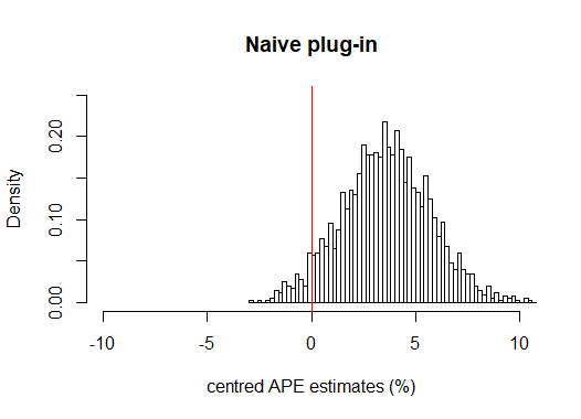
(a) APE estimates based on direct plug-in of lasso Logit coefficient estimates.

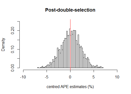
(b) APE estimates based on the proposed post-double-selection estimator.

Figure 1. Simulations for low-dimensional lasso Logit APE estimation based on $2,000$ iterations. Each iteration has sample size $n=200$. The dimensionality of covariates is set to be $p=10$. We set true parameter vector as $\beta^{0}=[.1,-1,1,0,...,0]$. Covariates $X$ are generated as i.i.d. zero-mean multivariate normal random vectors with Toeplitz covariance matrix $\Sigma$ with $\Sigma_{ij}=0.5^{|i-j|}$. Outcome variables are generated following $Y=\mathbbm{1}\{X^{\prime}\beta^{0}+U\}$ with i.i.d. $U$ following standard logistic distribution. The lasso estimations are implemented using R package glmnet with penalty selection algorithms discussed in Section 6.

To our knowledge, this is the first paper handling multiple testing and simultaneous confidence interval problems for more than a single APE under high-dimensional or big-data environments. In addition, cluster sampling with heterogeneous cluster sizes is allowed. Using the Neyman orthogonalization technique, we propose a new lasso-based post-double selection APE estimator. To accompany the main theoretical results, we propose valid nuisance parameter estimators as well as their practical tuning parameter selection algorithms that are compatible with our theory. To address the multiple-testing problem, we develop a new, simple-to-implement, multiplier cluster bootstrap. We provide simple algorithms for testing high-dimensional hypotheses and constructing simultaneously valid confidence intervals. Simulation studies suggest the proposed methods have favorable finite-sample performance. We illustrate the applicability of our theoretical results through examining a claim of Wu (2018) on the presence of genderally biased use of language following Wu’s text regression model using internet forum textual data from Economics Job Market Rumors (EJMR) forum - see the following section.

2. Motivation: Text Analysis and Gendered Language on the Internet

Text analysis using machine learning algorithms has become a useful alternative to the more traditional data analysis used in economics and other social sciences. Popular categories of text analysis models include text regression models, generative models, dictionary-based methods and word embeddings. The first two categories link attributes and word counts through conditional probabilities and, therefore, naturally relate to common econometric models. Notable examples of applications using text regression include stock prices prediction (e.g. Jegadeesh and Wu (2013)) and the Google Flu Trends, which is summarized in Ginsberg et al. (2009), among others. Gentzkow et al. (2019b) is a representative recent example for generative models applied to economics. For more details and applications, see Gentzkow et al. (2019a) for an up-to-date review.

Table 1. Top 10 most predictive words for female/male from Wu (2018)

Female		Male
Word	APE	Word	APE
Pregnancy	$0.292$	Knocking	$-0.329$
Hotter	$0.289$	Testosterone	$-0.204$
Pregnant	$0.258$	Blog	$-0.183$
Hp	$0.238$	Hateukbro	$-0.176$
Vagina	$0.228$	Adviser	$-0.175$
Breast	$0.220$	Hero	$-0.174$
Plow	$0.219$	Cuny	$-0.173$
Shopping	$0.207$	Handsome	$-0.166$
Marry	$0.207$	Mod	$-0.166$
Gorgeous	$0.201$	Homo	$-0.160$

(pronoun sample; a replication of Table 2 in Wu (2018))

Using a text regression model, Wu (2018) examines how women and men are discussed and depicted in the anonymous Economics Job Market Rumors forum. The author first extracted a list of female/male classifier vocabularies. According to Wu, a post is considered to be female if it contains any female classifier and male if it contains any male classifier. Let $Female_{i}$ be an indicator of whether post $i$ is female. $X_{i}$ denotes a vector of counts for each of the top 10,000 most common words (excluding all gender classifiers) that are present in gendered post $i$. Wu considers the text regression model with the logistic specification,

$${\mathrm{P}}(Female_{i}|X_{i})=\Lambda(X_{i}^{\prime}\beta)$$

where $\Lambda$ is the logistic function, using a lasso Logit procedure. The $Male$ counterpart is estimated analogously. For interpretability, Wu computes estimates for the APE for each of the $9,540$ words, where the APE for the word count of the $k$-th word is defined as

$$\text{APE}_{k}={\mathrm{E}}[\beta_{k}\Lambda^{\prime}(X_{i}^{\prime}\beta)].$$

Some top estimates of Wu’s are listed in Table 1. Based on these results, Wu concludes that the words that predict a post about a woman are typically about physical appearance or personal information, whereas those most predictive of a post about a man tend to focus on academic or professional characteristics.

Wu (2018) focuses on estimation. To further examine the magnitude and statistical significance of these estimates, the researcher may be interested in conducting hypotheses testing or constructing confidence intervals. To do so, several issues need to be carefully accounted for. First, as posts in EJMR data of Wu (2018) are sampled from different threads of various discussion topics, it is likely that posts coming from the same thread are highly correlated. Therefore, statistical testing should be conducted using a cluster robust inference method. Secondly, Wu (2018) highlights that females are often described with words about appearance or personal information. To formally quantify such statements, one may want to conduct multiple testing for APEs of a (potentially large) set of vocabularies related to appearance or personal information. Furthermore, in many cases, words with the same or close meaning are double-counted in this dataset, e.g. “attractive” and “attractiveness” or “homo”, “homosexual,” and “gay.” Thus, the researcher may want to consider a joint test that controls family-wise error rates for APEs of these words. This results in a multiple testing problem. Therefore, the testing procedure needs to be able to control the family-wise error rate while testing potentially many variables. To our best knowledge, no method in the literature is capable of addressing all these issues simultaneously. This paper attempts to provide a useful and easy-to-implement method that can be applied to such problems.

3. Background and Literature Review

3.1. Contributions

Our main contribution is to provide a theory for high-dimensional multiple-testing and simultaneous confidence intervals for APEs of binomial and fractional response regression models under clustered data. To our best knowledge, no results were previously available for this purpose. As a by-product, this paper also complements existing papers by proposing a practical method for studying low-dimensional APEs of interest under high-dimensional settings. Furthermore, cluster sizes are allowed to be heterogeneous - this is essential to our application as number of posts varies from thread to thread. Inference and construction of confidence intervals for such models are practically challenging; despite that methods are proposed in the literature, no simulation evidence for inference of even a single APE under lasso-regularization with these methods is available. In addition, we present practical and theoretically justified penalty choices for all the lasso estimators. Furthermore, easy-to-implement bootstrap procedures are also provided for inference/confidence intervals that hold valid, regardless of whether the researcher is interested in one or multiple APEs.

3.2. Relations to the Literature

The past decade has seen an explosive development in the literature of post-selection inference for lasso-based high-dimensional methods. This includes Belloni et al. (2012) for instrumental variable models, Belloni et al. (2014), Javanmard and Montanari (2014), Zhang and Zhang (2014), Farrell (2015), Caner and Kock (2018) and Athey et al. (2018) for linear regression/treatment effects models. Post-selection inference for generalized linear models such as Logit has been studied by van de Geer et al. (2014), Belloni et al. (2015), Belloni et al. (2016b), Belloni et al. (2017) and Belloni et al. (2018), to list a few. This line of research predominately focuses on regression coefficients of the generalized linear models rather than nonlinear functionals such as an APE. Recently, Chernozhukov et al. (2018b) study $L_{2}$-continuous functionals using lasso and Dantzig selector. While focusing on affine-functionals, they provide an extension of their method to nonlinear functionals. Their method makes use of a linear Riesz representer to approximate the linearization of a nonlinear functional, which differs from our approach. In addition, all of the aforementioned papers are based on i.i.d. or independent sampling assumptions. On the other hand, there are some results available for high-dimensional linear panel data. This includes Belloni et al. (2016a), Kock (2016) and Kock and Tang (2015).

Cluster-robust inference under various fixed-dimensional parametric settings has been well-studied and widely applied in the literature. See Wooldridge (2010) and Cameron and Miller (2015) for textbook treatment and comprehensive reviews. There has been recent literary focus on cluster-robust bootstrap inference. This includes Kline and Santos (2012), Hagemann (2017), MacKinnon and Webb (2017) and Djogbenou et al. (2019), among others. These results cannot be generalized in a straightforward manner to high-dimensional settings as the delta-method does not, in general, hold in an asymptotic framework with increasing dimensionality, see Caner (2017) for more details.

APE for binomial/fractional regression models has been discussed extensively in the literature (cf Chamberlain (1984), Wooldridge (2005) and Wooldridge (2019), etc). Inference for APEs of lasso-based binomial regression models are first studied by Wooldridge and Zhu (2017) under a short (balanced) panel data setting. They make use of a single-selection step with a lasso Probit estimator and propose a de-biased estimator for a single APE and obtain asymptotic normality. More recently, Hirshberg and Wager (2018) highlight the estimator of Wooldridge and Zhu (2017) for its requirement of a “soft” beta-min assumption that rules out regularization bias asymptotically. For i.i.d. data, Hirshberg and Wager (2018) provide an alternative augmented minimax estimator based on the novel framework for linear functionals developed in Hirshberg and Wager (2017). However, no variance estimator for this approach is proposed. Also, the aforementioned results are available only for a single APE; multiple testing and simultaneous confidence intervals for more than one APE remain unavailable. In addition, implementing inference for even a single APE under such settings presents practical challenges; to our best knowledge, there has been no simulation evidence presented for the proposed estimators in the aforementioned papers.

This paper aims to address all the aforementioned issues simultaneously. To do so, we extend the general framework for i.i.d. data developed in the important works of Belloni et al. (2015) and Belloni et al. (2018) to allow for cluster sampling and adapt it to the studies of APEs. The pointwise/simultaneous inference and confidence intervals are based on a multiplier cluster bootstrap which is built upon the high-dimensional central limit theorem of Chernozhukov et al. (2013).

3.3. Notations

Denote $(\Omega,\mathcal{A})$ the underlying measurable space and for each $G\in\mathbb{N}$, $\mathcal{P}_{G}$ is a set of probability measures ${\mathrm{P}}\in\mathcal{P}_{G}$ defined on $\mathcal{A}$. Consider triangular array data $\{W^{G}_{g}:g=1,...,G,G=1,2,3,...\}$ defined on probability space $(\Omega,\mathcal{A},{\mathrm{P}})$, where ${\mathrm{P}}$ depends on $G$ through $\mathcal{P}_{G}$. Each $W^{G}_{g}=\{W^{G}_{ig}:1\leq i\leq n_{g}\}$, is a random vector that is independent across $g$, but not necessarily identically distributed. All parameters that characterize the distribution of $\{W^{G}_{g};g=1,...,G\}$ are implicitly indexed by ${\mathrm{P}}_{G}$ and thus by $G$. This dependence is henceforth omitted for simplicity. $W_{ig}=(Y_{ig},X_{ig}^{\prime})^{\prime}$ takes values in $\mathbb{R}^{p+1}$. For each $g\leq G$, $G\in\mathds{N}$, the deterministic size of cluster $n_{g}$ satisfies $1\leq n_{g}\leq\bar{n}$ for a constant $\bar{n}$ independent of $G$. Therefore, for $i$ such that $n_{g}<i\leq\bar{n}$, we can set $W_{ig}=0$ and thus each $W_{g}$ can be represented as a $\bar{n}(p+1)$-dimensional random vector. Let ${\mathrm{E}}_{\mathrm{P}}$ be the expectation with respect to law ${\mathrm{P}}$.

For a vector $\beta$, the $k$-th component is denoted as $\beta_{k}$. For vectors, denote the $\ell_{1}$-norm as $\|\cdot\|_{1}$, ${l}_{2}$-norm as $\|\cdot\|$, $\ell_{\infty}$-norm as $\|\cdot\|_{\infty}$, and the “$\ell_{0}$-norm” as $\|\cdot\|_{0}$ to denote the number of non-zero components. For a matrix $A$, let $A^{\prime}$ be the transpose of $A$. For $1\leq q<\infty$, $\|A\|_{q}$ denotes the induced ${l}_{q}$-norm and $\|A\|_{\infty}=\max_{1\leq j,k\leq p}|A_{j,k}|$. For a vector $\delta\in{\mathbb{R}}^{p}$ and given data, $\|X_{ig}^{\prime}\delta\|_{G}=\sqrt{\frac{1}{G}\sum_{g=1}^{G}\sum_{i=1}^{n_{g}}(X_{ig}^{\prime}\delta)^{2}}$ denotes the prediction norm of $\delta$. Let $e_{j}$ be the $j$-th vector of the standard basis for $\mathbb{R}^{p}$. Given a vector $\delta\in{\mathbb{R}}^{p}$, and a set of indices $T\subseteq\{1,\ldots,p\}$, denote $\delta_{T}\in{\mathbb{R}}^{p}$ the vector such that $(\delta_{T})_{j}=\delta_{j}$ if $j\in T$ and $(\delta_{T})_{j}=0$ if $j\notin T$. The support of $\delta$ is defined as ${\rm support}(\delta)=\{j\in\{1,...,p\}:\delta_{j}\neq 0\}$. We denote $a\vee b=\max\{a,b\}$, and $a\wedge b=\min\{a,b\}$. The notaion $[k]=\{1,...,k\}$ is used for $k\in\mathbbm{N}$. We use $c$, $C$ to denote strictly positive constants that is independent of $G$ and ${\mathrm{P}}\in\mathcal{P}_{G}$. Their values may change at each presence. The notation $a_{G}\lesssim b_{G}$ denotes $a_{G}\leq Cb_{G}$ for all $G$ and some $C>0$ that does not depend on $G$. $a_{G}=o(1)$ means that there exists a sequence $(b_{G})_{G\geq 1}$ of positive numbers that do not depend on ${\mathrm{P}}\in\mathcal{P}_{G}$ for all $G$ such that $|a_{G}|\leq b_{G}$ for all $G$ and $b_{G}=o(1)$ as $G$ converges to zero. $a_{G}\lesssim_{P}b_{G}$ means that for any $\epsilon>0$, there exists $C$ such that ${\mathrm{P}}_{\mathrm{P}}(a_{G}>Cb_{G})\leq\epsilon$ for all $G$. Throughout the paper we assume $G\geq 3$.

3.4. Outline

The rest of the paper is structured as follows. In Section 4, an overview of the method and algorithms are given. Section 5 contains the main asymptotic results. Section 6 covers algorithms for penalty choices and the auxiliary results for theoretical performance of nuisance parameters. Results of simulation studies are demonstrated in Section 7. In Section 8, we apply the proposed method to conduct simultaneous testing to verify a statement about gendered language in Wu (2018). We concludes in Section 9. All the mathematical proofs and additional details are delegated to the appendix.

4. An Overview

Recall that $W_{ig}=(Y_{ig},X^{\prime}_{ig})^{\prime}$. Suppose that the researcher observes data sampled from $G$ clusters, $\{W_{ig}:i=1,...,n_{g},\>g=1,...,G\}$. Each cluster size $n_{g}$ is considered non-random, and $1\leq n_{g}\leq\bar{n}<\infty$ for a constant $\bar{n}$ that does not depend on $G$. Denote $n=\sum_{g=1}^{G}n_{g}$. Throughout the paper, we assume that the conditional expectation of $Y$ given $X$ follows the following single-index structure

$${\mathrm{E}}_{\mathrm{P}}(Y_{ig}|X_{ig})=\Lambda(X^{\prime}_{ig}\beta^{0}).$$

for each cluster $g$. Any $W_{i_{1}g},W_{i_{2}g}$ can be arbitrarily correlated while any $W_{i_{1}g_{1}},W_{i_{2}g_{2}}$ are independent if $g_{1}\neq g_{2}$. The dimensionality of $\beta^{0}$ is allowed to increase with $G$. This is the population-averaged approach as $\beta^{0}$ represents an averaged parameter after integrating out heterogeneity. The target parameter is the APE with respect to the $k$-th continuous covariate of interest,

$$\text{APE}_{k}={\mathrm{E}}_{\mathrm{P}}\left[\frac{1}{n}\sum_{g=1}^{G}\sum_{i=1}^{n_{g}}\beta^{0}_{k}\Lambda^{\prime}(X^{\prime}_{ig}\beta^{0})\right]$$

where $\Lambda^{\prime}$ stands for the derivative of $\Lambda$. As $n_{g}\leq\bar{n}$, it suffices to consider $\alpha_{k}$, the rescaled APE defined as

$$\alpha_{k}= {\mathrm{E}}_{\mathrm{P}}\left[\frac{1}{G}\sum_{g=1}^{G}\sum_{i=1}^{n_{g}}\beta^{0}_{k}\Lambda^{\prime}(X^{\prime}_{ig}\beta^{0})\right].$$

4.1. Estimation and Inference Procedures

We now summarize the estimation, inference and construction of simultaneous confidence intervals procedures based on the theoretical results to be presented in Section 5 and 6 ahead. First, we describe the procedures for computing the proposed APE estimators. Set $\alpha_{k}$ as the parameter of interest. The post-double-selection estimator for $\alpha_{k}$ is defined as

$$\widetilde{\alpha}_{k}=\frac{1}{G}\sum_{g=1}^{G}\sum_{i=1}^{n_{g}}\check{\beta}^{k}_{k}\Lambda^{\prime}(X_{ig}^{\prime}\check{\beta}^{k})$$ (4.1)

where $\check{\beta}^{k}$ is the pooled Logit estimate with its support restricted to the set of covariates

$$\widetilde{T}_{k}=\{k\}\cup{\rm support}(\widehat{\beta})\cup{\rm support}(\widehat{\zeta}^{k})\cup{\rm support}(\widehat{\gamma}^{k}),$$ (4.2)

and $\widehat{\beta}$, $\widehat{\zeta}^{k}$ and $\widehat{\gamma}^{k}$ are nuisance parameter estimators to be defined below. Therefore, once $\widetilde{T}_{k}$ is obtained, estimation of $\widetilde{\alpha}_{k}$ becomes a standard pooled Logit problem.

Suppose that we have some generic penalty tuning parameters $\lambda$, $\lambda^{\gamma}_{k}$ and $\lambda_{k}^{\zeta}$ and, in addition, $\widehat{\Psi}$, $\widehat{\Psi}^{\gamma}_{k}$, $\widehat{\Psi}_{k}^{\zeta}$, diagonal normalization matrices of dimensions $p$, $p-1$ and $p$, respectively. Formal and theoretically justified choices of these objects are delayed to Section 6.

First, $\widehat{\beta}$ and its two post-lasso counterparts are defined as

$$\widehat{\beta}\in\underset{\beta\in\mathbb{R}^{p}}{\text{argmin}}\>\frac{1}{G}\sum_{g=1}^{G}\sum_{i=1}^{n_{g}}\{-Y_{ig}X_{ig}^{\prime}\beta+\log(1+\exp(X^{\prime}_{ig}\beta)\,)\}+\frac{\lambda}{G}\|\widehat{\Psi}\beta\|_{1},$$ (4.3)

$$\widetilde{\beta}\in\underset{\beta\in\mathbb{R}^{p}:{\rm support}(\beta)\subset{\rm support}(\widehat{\beta})}{\text{argmin}}\>\frac{1}{G}\sum_{g=1}^{G}\sum_{i=1}^{n_{g}}\{-Y_{ig}X_{ig}^{\prime}\beta+\log(1+\exp(X^{\prime}_{ig}\beta)\,)\},$$ (4.4)

$$\widetilde{\beta}^{k}\in\underset{\beta\in\mathbb{R}^{p}:{\rm support}(\beta)\subset{\rm support}(\widehat{\beta}_{-k})}{\text{argmin}}\>\frac{1}{G}\sum_{g=1}^{G}\sum_{i=1}^{n_{g}}\{-Y_{ig}X_{ig}^{\prime}\beta+\log(1+\exp(X^{\prime}_{ig}\beta)\,)\}.$$ (4.5)

Using the above post-lasso estimates, we compute $\widehat{f}^{2}_{ig}=\Lambda^{\prime}(X_{ig}^{\prime}\widetilde{\beta})$ and $\widehat{S}_{ig}^{k}=\widetilde{\beta}^{k}_{k}\cdot\{1-2\Lambda(X_{ig}^{\prime}\widetilde{\beta})\}$. Throughout the rest of this paper, denote $D^{j}_{ig}=X_{ig,j}$, the $j$-th component of $X_{ig}$, and $X^{j}_{ig}=X_{ig,-j}^{\prime}$, the remaining $p-1$ variables. Using these quantities, the remaining two nuisance parameter estimates can be obtained as

$$\widehat{\gamma}^{k}=\>\underset{\gamma\in{\mathbb{R}}^{p-1}}{\rm argmin}\>\frac{1}{G}\sum_{g=1}^{G}\sum_{i=1}^{n_{g}}\widehat{f}^{2}_{ig}(D^{k}_{ig}-X^{k\prime}_{ig}\gamma)^{2}+2\frac{\lambda_{k}^{\gamma}}{G}\|\widehat{\Psi}_{k}^{\gamma}\gamma\|_{1},$$ (4.6)

$$\widehat{\zeta}^{k}=\>\underset{\zeta\in{\mathbb{R}}^{p}}{\rm argmin}\>\frac{1}{G}\sum_{g=1}^{G}\sum_{i=1}^{n_{g}}\widehat{f}^{2}_{ig}(\widehat{S}^{k}_{ig}-X^{\prime}_{ig}\zeta)^{2}+2\frac{\lambda_{k}^{\zeta}}{G}\|\widehat{\Psi}^{\zeta}_{k}\zeta\|_{1}.$$ (4.7)

Now $\widetilde{T}_{k}$ can be calculated following (4.2) and thus

$$\check{\beta}^{k}= \underset{\beta\in\mathbb{R}^{p}:\beta_{j}=0\text{ for all }j\in\widetilde{T}^{c}_{k}}{\rm argmin}\;\frac{1}{G}\sum_{g=1}^{G}\sum_{i=1}^{n_{g}}\{-Y_{ig}X_{ig}^{\prime}\beta+\log(1+\exp(X^{\prime}_{ig}\beta)\,)\},$$ (4.8)

and $\widetilde{\alpha}_{k}$ can be obtained following equation (4.1).

Suppose that the researcher is interested in $\alpha_{k}$ for a set of continuous covariates with $k\in A$ for an index set $A\subset[p]$. We present a concrete estimation procedure as the following algorithm.

Algorithm 4.1 (Post-double-selection estimator).

For each $k\in A$,

1. Run lasso and post-lasso Logit to compute $\widetilde{\beta}$ following (4.3) and (4.4).

2. Define generated weights $\widehat{f}^{2}_{ig}=\Lambda^{\prime}(X_{ig}^{\prime}\widetilde{\beta})$.

3. Run lasso to compute $\widehat{\gamma}^{k}$ following (4.6).

4. Run lasso to compute $\widehat{\zeta}^{k}$ following (4.7).

5. Let $\widetilde{T}_{k}=\{k\}\cup{\rm support}(\widehat{\beta})\cup{\rm support}(\widehat{\zeta}^{k})\cup{\rm support}(\widehat{\gamma}^{k})$ and compute $\check{\beta}^{k}$ following (4.8).

6. Compute plug-in estimator $\widetilde{\alpha}_{k}$ following (4.1).

Remark 4.1.

The post-double-selection estimator is theoretically related to the post-double-selection estimators for linear models in Belloni et al. (2014) and for Logit regression coefficients in Belloni et al. (2016b) and Belloni et al. (2018). However, because our target parameters of interest are APEs, the nonlinear transformations of high-dimensional nuisance parameters, rather than regression coefficients themselves, the structure of our nuisance parameters are fundamentally different. Estimation of these nuisance parameters requires different strategies and therefore presents extra challenges. We discuss the theory of nuisance parameters estimation in Section 6.

For inference, let us define the post-lasso counterparts of $\widehat{\gamma}^{k}$ and $\widehat{\zeta}^{k}$

$$\widetilde{\gamma}^{k}= \underset{{\rm support}(\gamma)\subset{\rm support}(\widehat{\gamma}^{k})}{\rm argmin}\frac{1}{G}\sum_{g=1}^{G}\sum_{i=1}^{n_{g}}\widehat{f}^{2}_{ig}(D^{k}_{ig}-X^{k}_{ig}\gamma)^{2},$$ (4.9)

$$\widetilde{\zeta}^{k}= \underset{{\rm support}(\zeta)\subset{\rm support}(\widehat{\zeta}^{k})}{\rm argmin}\frac{1}{G}\sum_{g=1}^{G}\sum_{i=1}^{n_{g}}\widehat{f}^{2}_{ig}(\widehat{S}^{k}_{ig}-X^{\prime}_{ig}\zeta)^{2},$$ (4.10)

and the nuisance parameter estimate

$$\widetilde{\theta}^{k}=[-\widetilde{\gamma}^{k}_{1},...,-\widetilde{\gamma}^{k}_{k-1},1,-\widetilde{\gamma}^{k}_{k},...,-\widetilde{\gamma}^{k}_{p-1}]^{\prime}\cdot\left\{\frac{1}{G\widehat{\tau}_{k}^{2}}\sum_{g=1}^{G}\sum_{i=1}^{n_{g}}\widehat{f}_{ig}^{2}\right\},$$ (4.11)

where each $\widehat{\tau}^{2}_{k}$ is calculated using

$$\widehat{\tau}_{k}^{2}:=\frac{1}{G}\sum_{g=1}^{G}\sum_{i=1}^{n_{g}}\widehat{f}_{ig}^{2}(D^{k}_{ig}-X^{k}_{ig}\widetilde{\gamma}^{k})^{2}.$$ (4.12)

Define the additional nuisance parameter estimate

$$\widetilde{\mu}^{k}=\widetilde{\zeta}^{k}+\widetilde{\theta}^{k}.$$ (4.13)

Finally, define the variance estimate as

$$\widetilde{\sigma}^{2}_{k}= \frac{1}{G}\sum_{g=1}^{G}\left\{\sum_{i=1}^{n_{g}}\left(\widetilde{\alpha}_{k}\left(\frac{G}{n}\right)-\widetilde{\beta}_{k}\Lambda^{\prime}(X_{ig}^{\prime}\widetilde{\beta})+\widetilde{\mu}^{k\prime}X_{ig}\{Y_{ig}-\Lambda(X_{ig}^{\prime}\widetilde{\beta})\}\right)\right\}^{2}.$$ (4.14)

We are now ready to introduce a procedure for simultaneous inference. Suppose that the null hypothesis of interest is

$$\text{H}_{0}:\alpha_{k}=\alpha_{k}^{0}\text{ for all $k\in A$}$$

for some values $(\alpha^{0}_{k})_{k\in A}$. We present a concrete simultaneous inference procedure as the following algorithm.

Algorithm 4.2 (Simultaneous inference via nultiplier cluster bootstrap).

For each $k\in A$,

1. Compute $\widetilde{\sigma}_{k}$ for $k\in A$ following (4.14).

2. Compute the test statistic $T=\max_{k\in[p]}\sqrt{G}\widetilde{\sigma}_{k}^{-1}|\widetilde{\alpha}_{k}-\alpha_{k}^{0}|.$

3. For each $k\in A$, compute $\widetilde{\mu}^{k}$ following (4.13).

4. Set the number of bootstrap iterations to $B$. For each $b\in[B]$, generate i.i.d. standard normal random variables $\{\xi^{b}_{g}\}_{g=1}^{G}$ independently from data.

5. For each $k\in A$ and $b\in[B]$, compute

   $$W^{b}=\max_{k\in A}\Big{|}\frac{1}{\sqrt{G}\widetilde{\sigma}_{k}}\sum_{g=1}^{G}\xi_{g}^{b}\sum_{i=1}^{n_{g}}\left(\widetilde{\alpha}_{k}\left(\frac{G}{n}\right)-\widetilde{\beta}^{k}_{k}\Lambda^{\prime}(X_{ig}^{\prime}\widetilde{\beta})+\widetilde{\mu}^{k\prime}X_{ig}\{Y_{ig}-\Lambda(X_{ig}^{\prime}\widetilde{\beta})\}\right)\Big{|}$$ (4.15)

   and $c_{a}$, the $(1-a)$-th quantile of $\{W^{b}\}_{b=1}^{B}$.

6. If $T>c_{a}$, reject $\text{H}_{0}$. Otherwise do not reject $\text{H}_{0}$.

Finally, we illustrate the procedure for constructing simultaneously valid confidence intervals with $(1-a)$ coverage probability for $\alpha_{k}$, $k\in A$.

Algorithm 4.3 (Simultaneous confidence intervals via multiplier cluster bootstrap).

For each $k\in A$,

1. Compute $\widetilde{\sigma}^{2}_{k}$ for $k\in A$ following (4.14).

2. Set the number of bootstrap iterations to $B$. For each $b\in[B]$, generate i.i.d. standard normal random variables $\{\xi^{b}_{g}\}_{g=1}^{G}$ independently from data.

3. For each $k\in A$ and $b\in[B]$, compute $W^{b}$ following (4.15) and $c_{a}$, the $(1-a)$-th quantile of $\{W^{b}\}_{b=1}^{B}$.

4. Compute simultaneous confidence intervals $I=\times_{k\in A}I_{k}$, where $I_{k}=\widetilde{\alpha}_{k}\pm\widetilde{\sigma}_{k}\cdot c_{a}/\sqrt{G}$.

Remark 4.2.

Note that it is also possible to conduct multiple testing and simultaneous confidence intervals without normalization (studentization). To do so, one simply follows every step in Algorithms 4.2 and 4.3 with $1$ in place of $\widehat{\sigma}_{k}$ for all $k$.

5. Main Theoretical Results

In this section, we present our main theoretical results for simultaneous inference and construction of confidence intervals. These results justify the validity of the algorithms proposed in Section 4. First, we introduce some notations. Recall

$${\mathrm{E}}_{\mathrm{P}}(Y_{ig}|X_{g})={\mathrm{E}}_{\mathrm{P}}(Y_{ig}|X_{ig})=\Lambda(X^{\prime}_{ig}\beta^{0}).$$

Define the Neyman orthogonal score for $\alpha_{k}$ by

$$\bar{\psi}_{k}(W_{ig},\alpha,\eta)= \alpha\cdot\frac{G}{n}-\beta_{k}\Lambda^{\prime}(X_{ig}^{\prime}\beta)+\mu^{\prime}X_{ig}\{Y_{ig}-\Lambda(X_{ig}^{\prime}\beta)\}$$ (5.16)

$$= \alpha\cdot\frac{G}{n}-\psi_{k}(W_{ig},\eta),$$

where $\psi_{k}(W_{ig},\eta)=\beta_{k}\Lambda^{\prime}(X_{ig}^{\prime}\beta)-\mu^{\prime}X_{ig}\{Y_{ig}-\Lambda(X_{ig}^{\prime}\beta)\}$. In addition, let the “ideal” population nuisance parameters for $\alpha_{k}$ be $\eta^{k}=(\beta^{0\prime},\mu^{k\prime})^{\prime}\in\mathbb{R}^{2p}$ with

$$\mu^{k}= \zeta^{k}+\theta^{k},$$ (5.17)

$$\zeta^{k}= \left\{{\mathrm{E}}_{\mathrm{P}}\left[\frac{1}{G}\sum_{g=1}^{G}\sum_{i=1}^{n_{g}}f^{2}_{ig}X_{ig}X_{ig}^{\prime}\right]\right\}^{-1}{\mathrm{E}}_{\mathrm{P}}\left[\frac{1}{G}\sum_{g=1}^{G}\sum_{i=1}^{n_{g}}f^{2}_{ig}X_{ig}S_{ig}^{k}\right],$$ (5.18)

$$\theta^{k}= \left\{{\mathrm{E}}_{\mathrm{P}}\left[\frac{1}{G}\sum_{g=1}^{G}\sum_{i=1}^{n_{g}}f^{2}_{ig}X_{ig}X_{ig}^{\prime}\right]\right\}^{-1}{\mathrm{E}}_{\mathrm{P}}\left[\frac{1}{G}\sum_{g=1}^{G}\sum_{i=1}^{n_{g}}f^{2}_{ig}e_{k}\right],$$ (5.19)

where $S^{k}_{ig}=\beta_{k}^{0}(1-2\Lambda(X_{ig}^{\prime}\beta^{0}))$ is an auxiliary regressor and $f^{2}_{ig}=\Lambda^{\prime}(X_{ig}^{\prime}\beta^{0})$ is a regression weight. Also denote the population nodewise regression coefficients for the $j$-th covariate as $\gamma^{j}$. We can also rewrite the population nuisance parameter regression coefficients $\zeta^{j}$ as a weighted projection of $S^{j}_{ig}$ on $X_{ig}$. Thus, we have the following

$$\gamma^{j}=\underset{\gamma\in\mathbb{R}^{p-1}}{\rm argmin}{\mathrm{E}}_{\mathrm{P}}\left[\frac{1}{G}\sum_{g=1}^{G}\sum_{i=1}^{n_{g}}f^{2}_{ig}(D^{j}_{ig}-X^{j}_{ig}\gamma)^{2}\right],$$ (5.20)

$$\zeta^{j}=\underset{\gamma\in\mathbb{R}^{p}}{\rm argmin}{\mathrm{E}}_{\mathrm{P}}\left[\frac{1}{G}\sum_{g=1}^{G}\sum_{i=1}^{n_{g}}f^{2}_{ig}(S^{j}_{ig}-X_{ig}\zeta)^{2}\right].$$ (5.21)

Denote the projection errors by $Z^{j}_{ig}=D^{j}_{ig}-X^{j}_{ig}\gamma^{j}$ and $\varepsilon^{j}_{ig}=S^{j}_{ig}-X_{ig}\zeta^{j}$. Let $q>4$ be a constant independent of $G$. Let $c_{1}$ and $C_{1}$ be some strictly positive constants independent of $G$. Furthermore, let $a_{G}=p\vee G$ and $\check{\delta}_{G}$ be a sequence of positive constants that converge to zero. $M_{G,1}\geq 1$ and $M_{G,2}\geq 1$ be some sequence of positive constants possibly diverging to infinity. $s=s_{G}$ is a non-decreasing sequence of constants. We make the follow assumptions.

Assumption 5.1 (Parameters).

The true parameters satisfy that

$$\|\beta^{0}\|_{2}+\max_{j\in[p]}\|\gamma^{j}\|_{2}+\max_{k\in[p]}\|\zeta^{k}\|_{2}\leq C_{1}.$$

Assumption 5.2 (Sparsity).

There exist vectors $\bar{\gamma}^{j}\in\mathbb{R}^{p-1}$ and $\bar{\zeta}^{k}\in\mathbb{R}^{p}$ for all $j,k\in[p]$ such that

$$\|\beta^{0}\|_{0}+\max_{j\in[p]}\|\bar{\gamma}^{j}\|_{0}+\max_{k\in[p]}\|\bar{\zeta}^{k}\|_{0}\leq s$$

and

$$\max_{j,k\in[p]}(\|\bar{\gamma}^{j}-\gamma^{j}\|_{2}\vee\|\bar{\theta}^{k}-\theta^{k}\|_{2}+s^{-1/2}\|\bar{\gamma}^{j}-\gamma^{j}\|_{1}\vee\|\bar{\zeta}^{k}-\zeta^{k}\|_{1})\leq C_{1}(s\log a_{G}/G)^{1/2}.$$

Remark 5.1.

Assumption 5.1 requires bounded $\ell_{2}$ norm of nuisance parameters, which is mild and standard in the lasso literature. The $\ell_{1}$ norm of the nuisance parameters are allowed to be growing with $G$. Note that we do not require exact sparsity of $\gamma^{j}$ and $\zeta^{k}$ in Assumption 5.2 since the exact sparsity of nodewise lasso coefficients could be more difficult to justify in many applications. Also, note that for each $j\in[p]$, we can without loss of generality assume $\bar{\gamma}^{j}=\gamma_{T}^{j}$, where $T={\rm support}(\gamma^{j})$. The same applies to $\bar{\zeta}^{k}$ and $\zeta^{k}$.

For the following assumption, define $U_{gk}=\bar{n}\cdot\max_{i\in[n_{g}]}|X_{ig,k}|$, $U_{g}=[U_{gk}]_{k\in[p]}$ and $V^{j}_{g}=\max_{i\in[n_{g}]}(|Z^{j}_{ig}|\vee|\varepsilon^{j}_{ig}|)$.

Assumption 5.3 (Covariates).

Suppose that there exist finite positive constants $c_{1}$, $C_{1}$ and $\check{\delta}_{G}=o(1)$ such that the following moment conditions hold for all $G$,

1. $\inf_{\|\xi\|_{2}=1}\left({\mathrm{E}}_{\mathrm{P}}[G^{-1}\sum_{g=1}^{G}\sum_{i=1}^{n_{g}}(f_{ig}X_{ig}^{\prime}\xi)^{2}]\bigwedge{\mathrm{E}}_{\mathrm{P}}[G^{-1}\sum_{g=1}^{G}(\sum_{i=1}^{n_{g}}\{Y_{ig}-\Lambda(X_{ig}^{\prime}\beta^{0})\}X_{ig}^{\prime}\xi)^{2}]\right)\geq c_{1}$.

2. $\min_{j,k}\left({\mathrm{E}}_{\mathrm{P}}[G^{-1}\sum_{g=1}^{G}(\sum_{i=1}^{n_{g}}f_{ig}^{2}Z^{j}_{ig}X_{ig,k})^{2}]\bigwedge{\mathrm{E}}_{\mathrm{P}}[G^{-1}\sum_{g=1}^{G}(\sum_{i=1}^{n_{g}}f_{ig}^{2}X_{ig,j}X_{ig,k})^{2}]\right)\geq c_{1}$.

3. $\max_{j,k}\{{\mathrm{E}}_{\mathrm{P}}[G^{-1}\sum_{g=1}^{G}|V^{j}_{g}U_{gk}|^{3}]\}^{1/3}\log^{1/2}a_{G}\leq\check{\delta}_{G}G^{1/6}$.

4. $\sup_{\|\xi\|_{2}=1}{\mathrm{E}}_{\mathrm{P}}[G^{-1}\sum_{g=1}^{G}(U_{g}^{\prime}\xi)^{4}]+\max_{j\in[p]}{\mathrm{E}}_{\mathrm{P}}[G^{-1}\sum_{g=1}^{G}(V^{j}_{g})^{4}]\leq C_{1}$.

5. $M_{G,1}\geq\{{\mathrm{E}}_{\mathrm{P}}[G^{-1}\sum_{g=1}^{G}\max_{j\in[p]}|V^{j}_{g}|^{2q}]\}^{1/2q}$.

6. $M_{G,1}^{4}s\log a_{G}\leq\check{\delta}_{G}G^{1/2-1/q}$.

7. $M_{G,2}\geq\{{\mathrm{E}}_{\mathrm{P}}[G^{-1}\sum_{g=1}^{G}\|U_{g}\|_{\infty}^{2q}]\}^{1/2q}$.

8. $M_{G,2}^{4}s\log a_{G}\leq\check{\delta}_{G}G^{1/2-1/q}$.

9. $(M_{G,1}^{2}\vee s\log^{2}a_{G})M_{G,2}^{4}s\leq\check{\delta}_{G}G^{1-3/q}$.

Assumption 5.4 (Sparse eigenvalues).

Let $\Delta(m)=\{\delta\in\mathbb{R}^{p}:\|\delta\|_{0}\leq m,\|\delta\|_{2}=1\}$. With probability at least $1-C(\log G)^{-1}$, we have

$$1\lesssim\min_{j\in[p]}\min_{\delta\in\Delta(Cs)}\frac{1}{G}\sum_{g=1}^{G}\sum_{i=1}^{n_{g}}(Z^{j}_{ig}X_{ig}^{\prime}\delta)^{2}\leq\max_{j\in[p]}\max_{\delta\in\Delta(Cs)}\frac{1}{G}\sum_{g=1}^{G}\sum_{i=1}^{n_{g}}(Z^{j}_{ig}X_{ig}^{\prime}\delta)^{2}\lesssim 1,$$

$$1\lesssim\min_{\delta\in\Delta(Cs)}\frac{1}{G}\sum_{g=1}^{G}\sum_{i=1}^{n_{g}}(X_{ig}^{\prime}\delta)^{2}\leq\max_{\delta\in\Delta(Cs)}\frac{1}{G}\sum_{g=1}^{G}\sum_{i=1}^{n_{g}}(X_{ig}^{\prime}\delta)^{2}\lesssim 1.$$

Remark 5.2.

Assumptions 5.1, 5.2, 5.3 are the cluster sampling counterpart of the Assumptions 3.1, 3.2, 3.4 and 3.5 of Belloni et al. (2018). To deal with APEs, however, we do need extra conditions on the growth of some moments that are listed below in the statement of Theorem 5.1. These growth conditions are satisfied when, for example, the covariates are sub-gaussian and/or uniformly bounded. When regressors are uniformly bounded, which is assumed in both Wooldridge and Zhu (2017) and Hirshberg and Wager (2018), the rate requirement would be $s\log p/G^{1/2}=o(1)$ ($s^{3/2}\log p/G^{1/2}=o(1)$ is required by Wooldridge and Zhu (2017)). Assumption 5.4 is analogous to condition SE in Belloni et al. (2016a) for the linear panel data model.

Theorem 5.1 (Main result).

Suppose that Assumptions 5.1, 5.2, 5.3, 5.4 hold, then

1. The following uniform Bahadur representation holds with probability at least $1-C(\log G)^{-1}$

   $$\sup_{{\mathrm{P}}\in\mathcal{P}_{G}}\max_{1\leq k\leq p}\Bigg{|}\sqrt{G}\sigma_{k}^{-1}(\widehat{\alpha}_{k}-\alpha_{k})-\frac{1}{\sqrt{G}}\sum_{g=1}^{G}\sum_{i=1}^{n_{g}}\varphi_{k}(W_{ig},\alpha_{k},\eta^{k})\Bigg{|}\lesssim\delta_{G},$$

   where $\varphi_{k}(W_{ig},\alpha,\eta)=-\bar{\psi}_{k}(W_{ig},\alpha,\eta)/\sigma_{k}$ and $\eta^{k}=(\beta^{0\prime},\mu^{k\prime})^{\prime}$.

2. Let $c_{W}(a)$ be the $a$-th quantile of $W$, we have, with probability at least $1-C(\log G)^{-1}$,

   $$\sup_{{\mathrm{P}}\in\mathcal{P}_{G}}\sup_{\alpha\in(0,1)}\Big{|}{\mathrm{P}}_{\mathrm{P}}\left(\max_{1\leq k\leq p}|\sqrt{G}\sigma_{k}^{-1}(\widehat{\alpha}_{k}-\alpha_{k})|\leq c_{W}(a)\right)-a\Big{|}=o(1).$$

   That is to say, the algorithms in Section 4 provide valid simultaneous inference and confidence intervals asymptotically.

A proof can be found in Section E.1 in the Appendix. Now, it remains to find a valid variance estimator. Recall the variance estimator $\widetilde{\sigma}_{k}^{2}$ defined in (4.14). Denote $\widetilde{\sigma}_{k}=\{\widetilde{\sigma}_{k}^{2}\}^{1/2}$.

Lemma 5.1 (Variance estimator).

Suppose that the conditions for Theorem 5.1 hold. Then

$$\max_{k\in[p]}|\widetilde{\sigma}_{k}-\sigma_{k}|\lesssim(\log a_{G})^{-1}$$

with probability at least $1-C(\log G)^{-1}$.

A proof can be found in Section E.2 in the Appendix.

6. Nuisance Parameters

Recall that the “ideal” nuisance parameter vector $\eta^{k}=(\beta^{0\prime},\mu^{k\prime})^{\prime}$, where

$$\mu^{k}= \left\{{\mathrm{E}}_{\mathrm{P}}\left[\frac{1}{G}\sum_{g=1}^{G}\sum_{i=1}^{n_{g}}f_{ig}^{2}X_{ig}X_{ig}^{\prime}\right]\right\}^{-1}\cdot{\mathrm{E}}_{\mathrm{P}}\left[\frac{1}{G}\sum_{g=1}^{G}\sum_{i=1}^{n_{g}}\left(\beta^{0}_{k}\Lambda^{\prime\prime}(X_{ig}^{\prime}\beta^{0})X_{ig}+\Lambda^{\prime}(X_{ig}^{\prime}\beta^{0})e_{k}\right)\right]=\zeta^{k}+\theta^{k}.$$

In this section, we propose estimators for these nuisance parameters as well as some theoretically justified choices of penalty tuning parameters. The choices here are based on the moderate deviation theory of self-normalized sums, which is first adapted for penalty selection of lasso by Belloni et al. (2012). Throughout this section, we fix a positive integer $\bar{m}\geq 1$ as the number of iterations used in the algorithms for choosing penalty tuning parameters.

6.1. Post-Lasso Logit and Estimation of $\beta^{0}$

We now establish an asymptotic theory for estimation of $\beta^{0}$, which plays a central role in estimation of APE. The identification of $\beta^{0}$ follows from quasi-maximum likelihood and the assumption of population-averaged approach ${\mathrm{E}}[Y_{ig}|X_{ig}]=\Lambda(X_{ig}^{\prime}\beta^{0})$. Define the negative partial log-likelihood function by

$$M(Y_{ig},X_{ig},\beta)=-\{Y_{ig}X_{ig}^{\prime}\beta-\log(1+\exp(X^{\prime}_{ig}\beta))\}.$$ (6.22)

Then, one has

$$\beta^{0}=\underset{\beta\in\mathbb{R}^{p}}{\text{argmin}}\>{\mathrm{E}}_{\mathrm{P}}\left[\frac{1}{G}\sum_{g=1}^{G}\sum_{i=1}^{n_{g}}M(Y_{ig},X_{ig},\beta)\right].$$

We propose the following algorithm for the choice of $\widehat{\Psi}$.

Algorithm 6.1 (Penalty choice: clustered Lasso logit $\beta^{0}$).

Define $\lambda=c\sqrt{G}\Phi^{-1}(1-\gamma/2p)$ and set $c=1.1$ and $\gamma=0.1/\log G$. For $m=0$, let

$$\widehat{l}_{j,0}=\frac{1}{2}\left\{\frac{1}{G}\sum_{g=1}^{G}\left(\sum_{i=1}^{n_{g}}n_{g}X^{2}_{ig,j}\right)\right\}^{1/2}$$

and for $1\leq m\leq\bar{m}$,

$$\widehat{l}_{j,m}=\left\{\frac{1}{G}\sum_{g=1}^{G}\left(\sum_{i=1}^{n_{g}}\{Y_{ig}-\Lambda(X_{ig}\widetilde{\beta})\}X_{ig,j}\right)^{2}\right\}^{1/2}$$

with $\widetilde{\beta}$ coming from iteration $m-1$. Let $\widehat{\Psi}={\rm diag}\{\widehat{l}_{j,m}:j\in[p]\}$.

The following result provides convergence rates of $\widetilde{\beta}$ and $\widetilde{\beta}^{k}$.

Theorem 6.1.

Suppose that the Assumption 5.1, 5.2, 5.3 and 5.4 are satisfied. If $\check{\delta}_{G}^{2}\log a_{G}=o(1)$, then with penalty chosen according to Algorithm (6.1), with probability $1-\gamma$, $\gamma=O(1/\log G)$,

$$\|\widetilde{\beta}-\beta^{0}\|_{1}\vee\max_{k\in[p]}\|\widetilde{\beta}^{k}-\beta^{0}\|_{1}\lesssim\sqrt{\frac{s^{2}\log a_{G}}{G}}\text{ and }\|\widetilde{\beta}-\beta^{0}\|_{2}\vee\max_{k\in[p]}\|\widetilde{\beta}^{k}-\beta^{0}\|_{2}\lesssim\sqrt{\frac{s\log a_{G}}{G}}.$$

A proof can be found in Section F.1 in the Appendix.

6.2. Weighted Post-Lasso with Estimated Weights

We now establish asymptotic theory for weighted post-lasso with estimated weights that will be essential for Sections 6.3 and 6.4. We propose the following algorithm for the choices of penalty tuning parameters.

Algorithm 6.2 (Penalty choice: weighted clustered Lasso $\gamma^{j}$).

Define $\lambda^{\gamma}=c\sqrt{G}\Phi^{-1}(1-\gamma/2p(p-1))$ and set $c=1.1$ and $\gamma=0.1/\log G$. For each $j\in[p]$, for $m=0$, set

$$\widehat{l}_{jk,0}= 2\max_{g\in[G]}\max_{i\in[n_{g}]}|\widehat{f}_{ig}X_{ig,k}|\left\{\frac{1}{G}\sum_{g=1}^{G}\left(\sum_{i=1}^{n_{g}}\widehat{f}_{ig}D^{j}_{ig}\right)^{2}\right\}^{1/2}$$

and $1\leq m\leq\bar{m}$,

$$\widehat{l}_{jk,m}= 2\left\{\frac{1}{G}\sum_{g=1}^{G}\left(\sum_{i=1}^{n_{g}}\widehat{f}_{ig}^{2}(D^{j}_{ig}-X^{j}_{ig}\widetilde{\gamma}^{j})X^{j}_{ig,k}\right)^{2}\right\}^{1/2}$$

and $\widehat{\Psi}^{\gamma}_{j}={\rm diag}\{\widehat{l}_{jk,m}:k\in[p-1]\}$.

The following result provides convergence rates of $\widetilde{\gamma}^{j}$, which plays an important role in Section 6.3.

Theorem 6.2.

Suppose that Assumption 5.1, 5.2, 5.3, 5.4 are satisfied and if $\check{\delta}_{G}^{2}\log a_{G}=o(1)$, then with penalty chosen according to Algorithm (6.2), with probability $1-\gamma$, $\gamma=O(1/\log G)$

$$\max_{j\in[p]}\|\widetilde{\gamma}^{j}-\gamma^{j}\|_{1}\lesssim\sqrt{\frac{s^{2}\log a_{G}}{G}}\>\text{ and }\>\max_{j\in[p]}\|\widetilde{\gamma}^{j}-\gamma^{j}\|_{2}\lesssim\sqrt{\frac{s\log a_{G}}{G}}.$$

A proof can be found in Section F.2 in the Appendix.

6.3. Nodewise Post-Lasso and Estimation of $\theta^{k}$

Now we provide estimators for $\theta^{k}$ that are built upon the method of cluster nodewise post-lasso estimator for approximately inverting a singular matrix. The theory developed here is based on applying the weighted post-lasso with estimated weights from Belloni et al. (2018) to the panel nodewise regressions of Kock (2016). Recall that each nuisance parameter vector $\theta^{k}$ contains the matrix

$$\Theta:=\left\{{\mathrm{E}}_{\mathrm{P}}\left[\frac{1}{G}\sum_{g=1}^{G}\sum_{i=1}^{n_{g}}f^{2}_{ig}X_{ig}X^{\prime}_{ig}\right]\right\}^{-1}.$$

Its sample counterpart is not invertible if $p>n$ and could be very unstable if $p$ is only moderately larger than $n$. Here, we take advantage of Assumption 5.2 to construct a high quality approximate inverse estimate. Denote $\Theta_{j}$ for the $j$-th row written as a column vector. If we can find some reasonable estimator $\widehat{\Theta}_{k}$ for $\Theta_{k}$, then intuitively an estimator for $\theta^{k}$ can be defined as

$$\widetilde{\theta}^{k}=\widehat{\Theta}_{k}\cdot\frac{1}{G}\sum_{g=1}^{G}\sum_{i=1}^{n_{g}}\widehat{f}_{ig}^{2}.$$

We propose a cluster nodewise post-lasso procedure to estimate $\Theta$. Recall that the error $Z^{j}_{ig}=D^{j}_{ig}-X^{j}_{ig}\gamma^{j}$ which satisfies ${\mathrm{E}}_{\mathrm{P}}[\frac{1}{G}\sum_{g=1}^{G}\sum_{i=1}^{n_{g}}f^{2}_{ig}X^{j}_{ig}Z^{j}_{ig}]=0$. Define the error variance $\tau^{2}_{j}={\mathrm{E}}_{\mathrm{P}}[\frac{1}{G}\sum_{g=1}^{G}\sum_{i=1}^{n_{g}}f^{2}_{ig}(Z_{ig}^{j})^{2}]$. Some properties of $\tau_{j}^{2}$ can be found in Section G.1. Note that $\gamma^{j}$ has a sparse approximation $\bar{\gamma}^{j}$ under Assumption 5.1. Then, we can use post-lasso estimate $\widetilde{\gamma}^{j}$ for $\gamma^{j}$ from Section 6.2 and construct a $p\times p$ matrix $\widehat{C}$ by

$$\widehat{C}=\begin{bmatrix}1&-\widetilde{\gamma}^{1}_{1}&\dots&-\widetilde{\gamma}^{1}_{p-1}\\ -\widetilde{\gamma}^{2}_{1}&1&\dots&-\widetilde{\gamma}^{2}_{p-1}\\ \vdots&\vdots&\ddots&\vdots\\ -\widetilde{\gamma}^{p}_{1}&-\widetilde{\gamma}^{p}_{2}&\dots&1\end{bmatrix}.$$

That is, the off-diagonal spots of the $j$-th row of $\widehat{C}$ consist of components of $-\widetilde{\gamma}^{j}$ and the diagonal entries are set to $1$. Also, denote

$$\widehat{T}^{2}=\text{diag}\{\widehat{\tau}_{1}^{2},...,\widehat{\tau}_{p}^{2}\},$$

where $\widehat{\tau}_{j}^{2}$ is defined in (4.12). Now, the cluster nodewise post-lasso estimator for $\Theta$ is defined as

$$\widehat{\Theta}=\widehat{T}^{-2}\widehat{C},$$

which in turn gives the expression of (4.11). The following results provide validity of $\widehat{\Theta}$ and $\widetilde{\theta}^{k}$.

Lemma 6.1.

Suppose that the Assumption 5.1, 5.2, 5.3, 5.4 are satisfied. If $\check{\delta}_{G}^{2}\log a_{G}=o(1)$, then with penalty chosen according to Algorithm 6.2, with probability $1-\gamma$, $\gamma=O(1/\log G)$,

$$\max_{j\in[p]}\|\widehat{\Theta}_{j}-\Theta_{j}\|_{1}\lesssim\sqrt{\frac{s^{2}\log a_{G}}{G}}\text{ and }\max_{j\in[p]}\|\widehat{\Theta}_{j}-\Theta_{j}\|_{2}\lesssim\sqrt{\frac{s\log a_{G}}{G}}.$$

Theorem 6.3.

Suppose that all assumptions required by Lemma 6.1 are satisfied. Then, with probability $1-\gamma$, $\gamma=O(1/\log G)$, we have

$$\max_{k\in[p]}\|\widetilde{\theta}^{k}-\theta^{k}\|_{1}\lesssim\sqrt{\frac{s^{2}\log a_{G}}{G}}\text{ and }\max_{k\in[p]}\|\widetilde{\theta}^{k}-\theta^{k}\|_{2}\lesssim\sqrt{\frac{s\log a_{G}}{G}}.$$

Proofs for the above two results can be found in Sections F.4 and F.5 in the Appendix.

6.4. Weighted Post-Lasso and Estimation of $\zeta^{k}$

Recall that the nuisance parameters $\zeta^{k}$ is identified by

$$\zeta^{k}=\underset{\zeta\in\mathbb{R}^{p}}{\text{argmin}}\>{\mathrm{E}}_{\mathrm{P}}\left[\frac{1}{G}\sum_{g=1}^{G}\sum_{i=1}^{n_{g}}f_{ig}^{2}(S_{ig}^{k}-X^{\prime}_{ig}\zeta)^{2}\right].$$

We propose the following algorithm for choice of the penalty tuning parameters.

Algorithm 6.3 (Penalty Choice: Weighted Clustered Lasso $\zeta^{k}$).

Define $\lambda^{\zeta}_{j}=c\sqrt{G}\Phi^{-1}(1-\gamma/2p^{2})$ and set $c=1.1$ and $\gamma=0.1/\log G$. For each $k\in[p]$, for $m=0$, set

$$\widehat{l}_{kj,0}= 2\max_{g\in[G]}\max_{i\in[n_{g}]}|\widehat{f}_{ig}X_{ig,j}|\left\{\frac{1}{G}\sum_{g=1}^{G}\left(\sum_{i=1}^{n_{g}}\widehat{f}_{ig}\widehat{S}^{k}_{ig}\right)^{2}\right\}^{1/2}$$

and $1\leq m\leq\bar{m}$,

$$\widehat{l}_{kj,m}= 2\left\{\frac{1}{G}\sum_{g=1}^{G}\left(\sum_{i=1}^{n_{g}}\widehat{f}_{ig}^{2}(\widehat{S}^{k}_{ig}-X_{ig}^{\prime}\widetilde{\zeta}^{k})X_{ig,j}\right)^{2}\right\}^{1/2}$$

and $\widehat{\Psi}^{\zeta}_{k}={\rm diag}\{\widehat{l}_{kj,m}:j\in[p]\}$.

The following result provides convergence rates of $\widetilde{\zeta}^{k}$.

Corollary 6.1.

Suppose that Assumptions 5.1, 5.2, 5.3, 5.4 hold. If $\check{\delta}_{G}^{2}\log a_{G}=o(1)$, then with penalty chosen according to Algorithm 6.3, with probability $1-\gamma$, $\gamma=O(1/\log G)$,

$$\max_{k\in[p]}\|\widetilde{\zeta}^{k}-\zeta^{k}\|_{1}\lesssim\sqrt{\frac{s^{2}\log a_{G}}{G}}\text{ and }\max_{k\in[p]}\|\widetilde{\zeta}^{k}-\zeta^{k}\|_{2}\lesssim\sqrt{\frac{s\log a_{G}}{G}}.$$

A proof can be found in Section F.3 in the Appendix.

7. Simulation Studies

In this section, we conduct simulation studies to investigate the finite-sample performance of the proposed procedures. Set the number of total observations to $n$, and each observation is then randomly assigned into $G_{0}$ clusters. The empty clusters, if they exist, are then discarded and thus $G\leq G_{0}$. For DGP1, let the number of covariates for each observation be $p=1.5\cdot G_{0}$ and

$$\beta^{0}=[1,\beta_{2},1/3,1/4,1/5,..,1/19,1/20,0,...,0]^{\prime}\in\mathbb{R}^{p}.$$

The first component of each covariate vector is set to $1$ and the rest of the subvector, $X_{ig,-1}$, can be decomposed into an idiosyncratic part $X^{1}_{ig}$ and a cluster-wise component $X^{2}_{g}$ as

$$X_{ig,-1}=X^{1}_{ig}+X^{2}_{g}$$

and both $X^{1}_{ig}$ and $X^{2}_{g}$ are i.i.d. following a multivariate normal distribution with mean $0$ and a Toeplitz covariance matrix:

$$\Sigma_{ij}(\rho):=\rho^{|i-j|},\;\rho=0.1,\,0.3,\,0.5,\,0.7,\,0.9,\;i,j,\in[p-1].$$

So the larger $\rho$ is, the more correlated the covariates are. The outcome variable is generated by

$$\qquad Y_{ig}=\mathbbm{1}\left\{X_{ig}^{\prime}\beta^{0}+U_{ig}>0\right\},$$

where the error term can also be decomposed into an idiosyncratic term and a cluster-wise term as

$$U_{ig}=\Lambda\left(\Phi^{-1}(U^{1}_{ig}+U^{2}_{g})\right),$$

where both $U^{1}_{ig}$ and $U^{2}_{g}$ are i.i.d. following the normal $N(0,1/2)$ distribution. Thus, $U_{ig}$ is a standard logistic distribution. Thus both covariates and errors are correlated within each cluster. To consider “outliers” and substantial skew and kurtosis in marginal distribution of independent variables, we also consider alternative DGPs inspired by Kline and Santos (2012) by setting $X^{1}_{ig}$ and $X^{2}_{g}$ to follow a mixture between two distributions, $N(0,\Sigma(\rho))$ with probability 0.9 and a $N(0,\Sigma(\rho))-1.5\times N(1,\Sigma(\rho))$ with probability $0.1$.

Table 2. List of DGPs in Simulation Studies.

DGP	Descriptions
M1	$X^{1}_{ig},\,X^{2}_{g}\sim N(0,\Sigma(\rho))$ with $\rho=0.1$
M2	Same as M1 except $\rho=0.3$
M3	Same as M1 except $\rho=0.5$
M4	Same as M1 except $\rho=0.7$
M5	Same as M1 except $\rho=0.9$
M6	$X^{1}_{ig},\,X^{2}_{g}\sim\left(N(0,\Sigma(\rho))-1.5*B(1,0.1)*N(1,\Sigma(\rho))\right)$ with $\rho=0.1$
M7	Same as M6 except $\rho=0.3$
M8	Same as M6 except $\rho=0.5$
M9	Same as M6 except $\rho=0.7$
M10	Same as M6 except $\rho=0.9$

Note that for the DGPs with high $\rho$ values, such as M4, M5, M9 and M10, the approximate sparsity conditions in Assumption 5.1 are violated. We conduct three sets of simulations. First we examine one-dimensional confidence interval coverage for $\alpha_{2}$ with true underlying $\beta_{2}\in\{0,0.25,0.5,0.75,1\}$. Our second goal is to construct simultaneous confidence intervals that control the family-wise error rate for $\alpha_{k}$ for $k\in A$, $A$ is set to be

$$A_{1}=\{2\},\,A_{2}=\{2,3\},\,A_{3}=\{2,3,4\},\,A_{5}=\{2,3,...,6\},\,A_{10}=\{2,3,...,10\},\,A_{20}=\{2,3,...,20\},$$

$$A_{30}=\{2,3,...,31\},\,A_{40}=\{2,3,...,41\},\,A_{50}=\{2,3,...,51\},\,A_{100}=\{2,3,...,101\},$$

where the APE with respect to the intercept is always omitted. In this group of simulations, we set $\beta_{2}=0.5$. Finally, we examine the asymptotic behaviors of coverage probabilities of simultaneous intervals for $A_{10}$.

The estimation of all lasso and lasso Logit are conducted using R package glmnet and the penalty choices follow Algorithms 6.1, 6.2 and 6.3 in Section 6 with $\bar{m}=1$. For each iteration of the simulation, we set the number of bootstrap iterations to $B=600$. We then simulate $1,000$ times for each DGP. The simultaneous confidence intervals are constructed following Algorithm 4.3 and without normalization by $\widetilde{\sigma}_{k}$ for simplicity. The true $\alpha_{k}$ are computed using $3,000,000$ additional observations generated independently from data following the same marginal distribution as $X_{ig}$. The nominal coverage probability is set to be $0.95$. The results for one-dimensional confidence intervals are presented in Table 3.   

Table 3. Coverage probability for one-dimensional $95$% confidence intervals for $\alpha_{2}$ under each DGP with $G_{0}=200$, $n=500$ and $p=300$:

DGP	$\beta_{2}=0$	$\beta_{2}=.25$	$\beta_{2}=.5$	$\beta_{2}=.75$	$\beta_{2}=1$
M1	$0.953$	$0.935$	$0.943$	$0.959$	$0.972$
M2	$0.949$	$0.944$	$0.937$	$0.956$	$0.969$
M3	$0.939$	$0.938$	$0.941$	$0.951$	$0.968$
M4	$0.938$	$0.944$	$0.937$	$0.944$	$0.954$
M5	$0.928$	$0.931$	$0.928$	$0.940$	$0.923$
M6	$0.928$	$0.919$	$0.920$	$0.946$	$0.970$
M7	$0.921$	$0.920$	$0.912$	$0.926$	$0.957$
M8	$0.934$	$0.925$	$0.929$	$0.954$	$0.956$
M9	$0.926$	$0.929$	$0.933$	$0.941$	$0.958$
M10	$0.938$	$0.935$	$0.944$	$0.938$	$0.947$

We now illustrate the necessity of cluster robust method under many-small-cluster asymptotics. Consider DGP M1-M5. Suppose we implement observation-wise multiplier bootstrap (i.e. in each iternation, i.i.d. standard normal r.v.’s $\xi_{i}^{b}$ are generated for each observation) in place of the proposed multiplier cluster bootstrap. The results are presented in Table 4. One can see that in most cases, the non-cluster robust method is severely oversized while the multiplier cluster bootstrap has close to nominal coverage rates consistently.   

Table 4. Comparison of cluster robust and non-cluster robust methods’ coverage probability for one-dimensional $95$% confidence intervals for $\alpha_{2}$ under DGP M1-M5 with $G_{0}=200$, $n=500$ and $p=300$:

Cluster robust	$\beta_{2}=0$	$\beta_{2}=.25$	$\beta_{2}=.5$	$\beta_{2}=.75$	$\beta_{2}=1$
		DGP:	M1
Yes	$0.953$	$0.935$	$0.943$	$0.959$	$0.972$
No	$0.907$	$0.910$	$0.900$	$0.934$	$0.962$
		DGP:	M2
Yes	$0.949$	$0.944$	$0.937$	$0.956$	$0.969$
No	$0.913$	$0.899$	$0.898$	$0.933$	$0.943$
		DGP:	M3
Yes	$0.939$	$0.938$	$0.941$	$0.951$	$0.968$
No	$0.884$	$0.914$	$0.921$	$0.941$	$0.962$
		DGP:	M4
Yes	$0.938$	$0.944$	$0.937$	$0.944$	$0.954$
No	$0.885$	$0.924$	$0.901$	$0.929$	$0.936$
		DGP:	M5
Yes	$0.928$	$0.931$	$0.928$	$0.940$	$0.923$
No	$0.922$	$0.897$	$0.906$	$0.933$	$0.923$

We now present the coverage probabilities for simultaneous confidence intervals for different sets of covariates. For this part of experiments, we focus on models M1 to M5 with $\beta_{2}=0.5$. The results are shown in Table 5.

Table 5. Coverage probability for $95$% simultaneous confidence intervals for $\alpha_{k}$, $k\in A$ under each DGP with $G_{0}=200$, $n=500$ and $p=300$:

DGP	$A_{1}$	$A_{2}$	$A_{3}$	$A_{5}$	$A_{10}$	$A_{20}$	$A_{30}$	$A_{40}$	$A_{50}$	$A_{100}$
M1	$0.943$	$0.941$	$0.933$	$0.926$	$0.920$	$0.940$	$0.951$	$0.959$	$0.957$	$0.943$
M2	$0.937$	$0.945$	$0.932$	$0.930$	$0.907$	$0.927$	$0.917$	$0.920$	$0.940$	$0.950$
M3	$0.941$	$0.943$	$0.956$	$0.914$	$0.882$	$0.900$	$0.901$	$0.914$	$0.920$	$0.930$
M4	$0.937$	$0.928$	$0.925$	$0.876$	$0.865$	$0.863$	$0.865$	$0.891$	$0.897$	$0.925$
M5	$0.928$	$0.926$	$0.930$	$0.891$	$0.865$	$0.861$	$0.874$	$0.898$	$0.894$	$0.904$

As before, we now illustrate the need of cluster robust method in simultaneous inference. As Table 6 shows, the oversize problem of non-cluster robust method is aggravated in simultaneous inference.

Table 6. Comparison of cluster robust and non-cluster robust methods’ coverage probability for $95$% simultaneous confidence intervals for $\alpha_{k}$, $k\in A$ under each DGP with $G_{0}=200$, $n=500$ and $p=300$:

Cluster robust	$A_{1}$	$A_{2}$	$A_{3}$	$A_{5}$	$A_{10}$	$A_{20}$	$A_{50}$	$A_{100}$
			DGP:	M1
Yes	$0.943$	$0.941$	$0.933$	$0.926$	$0.920$	$0.940$	$0.957$	$0.943$
No	$0.900$	$0.896$	$0.877$	$0.852$	$0.842$	$0.839$	$0.785$	$0.788$
			DGP:	M2
Yes	$0.937$	$0.945$	$0.932$	$0.930$	$0.907$	$0.927$	$0.940$	$0.950$
No	$0.898$	$0.894$	$0.890$	$0.847$	$0.819$	$0.810$	$0.773$	$0.774$
			DGP:	M3
Yes	$0.941$	$0.943$	$0.956$	$0.914$	$0.882$	$0.900$	$0.920$	$0.930$
No	$0.921$	$0.890$	$0.861$	$0.851$	$0.796$	$0.706$	$0.730$	$0.753$
			DGP:	M4
Yes	$0.937$	$0.928$	$0.925$	$0.876$	$0.865$	$0.863$	$0.897$	$0.925$
No	$0.901$	$0.903$	$0.854$	$0.856$	$0.765$	$0.720$	$0.732$	$0.760$
			DGP:	M5
Yes	$0.928$	$0.926$	$0.930$	$0.891$	$0.865$	$0.861$	$0.894$	$0.904$
No	$0.906$	$0.906$	$0.869$	$0.831$	$0.764$	$0.766$	$0.775$	$0.775$

Finally, we investigate the asymptotic behaviors of the case with $A_{10}$, one of the worst-performing cases in the above simulations for simultaneous confidence intervals, to examine whether the performance improves as sample size increases. In this set of simulations, set $\beta_{2}=0.5$ for number of nominal clusters $G_{0}=200$, $400$, $600$ and $800$, $p=1.5\cdot G_{0}$, and $n=2.5\cdot G_{0}$. The results are presented in Table 7.

Table 7. Asymptotic behaviors of coverage probability for $95$% simultaneous confidence intervals for $\alpha_{k}$, $k\in A_{10}$ under each DGP:

DGP	$G_{0}=200$	$G_{0}=400$	$G_{0}=600$	$G_{0}=800$
M1	$0.920$	$0.914$	$0.930$	$0.945$
M2	$0.907$	$0.917$	$0.920$	$0.921$
M3	$0.882$	$0.894$	$0.898$	$0.903$
M4	$0.865$	$0.856$	$0.864$	$0.876$
M5	$0.865$	$0.859$	$0.847$	$0.857$

In all of the simulation experiments, the coverage probabilities are mostly reasonably close to the nominal coverage rate when $\rho$ is not close to one. When $\rho$ is high, the approximate sparsity of nuisance parameters in Assumption 5.1 is potentially violated. Thus some of the coverage probabilities deviate away from the nominal rate. In addition, the coverage probabilities improve as sample size increases. In summary, the outcomes of these experiments are consistent with our theoretical results.

8. Application: Testing Gendered Language on the Internet

In this section, we apply our method of simultaneous inference for APEs in the text regression model of Wu (2018) introduced in Section 2. We make use of the pronoun sample (gendered posts including either female or male pronouns) from Wu (2018). Following Wu, using the EJMR dataset, we exclude the same list of words from the 10,000, including all gender classifiers, plus names of non-economist celebrities. We conduct our analysis based on the subset of non-duplicate posts that are used as the test sample for selecting optimal probability threshold in the original paper (the posts with index labelled as test0) for classification of posts that contains both female and male classifiers. We consider only pronoun sample. This leaves 46,502 posts sampled from 31,739 threads and 9541 covariates that consists of an intercept and the word counts of 9,540 non-excluded vocabularies.

Wu (2018) highlights that posts about males include more academically and professionally oriented vocabularies, such as “adviser,” “supervisor,” and “Nobel.” To see the joint significance of these words’ APE in terms of predicting female, we test

$$\text{H}_{0}:\alpha_{\text{adviser }}=\alpha_{\text{supervisor}}=\alpha_{\text{nobel}}=0.$$

Following the penalty choices of Algorithms 6.1, 6.2 and 6.3, the estimates of APEs of these words calculated using Algorithm 4.1 are listed in Table 8. These estimates are qualitatively similar to the corresponding estimates in Wu (2018). Using multiplier cluster bootstrap with $10,000$ bootstrap iterations, we obtain the test results listed in Table 9. Note that under all three confidence levels, we reject the null hypothesis and the statistical evidence supports Wu’s statement .

Table 8. APE estimates for “adviser,” “supervisor,” and “Nobel.”

	adviser	supervisor	Nobel
APE estimate	$-0.1414$	$-0.1214$	$-0.1214$

Table 9. Multiple Testing Results under $1-\alpha\%$ Confidence level.

$\alpha$	MCB critical value	test statistic
$10\%$	$16.0889$	$25.1867$
$5\%$	$18.2870$	$25.1867$
$1\%$	$22.2930$	$25.1867$

9. Conclusion

In this paper, we study logistic average partial effects with lasso regularization when data is sampled under clustering. We proposed two valid estimators along with their theoretically justified lasso penalty choices. Based on these estimators, we provide easy-to-implement algorithms for simultaneous inference and confidence intervals and establish their asymptotic validity. Simulation studies demonstrate that the proposed procedures work as predicted by the theory in finite sample. We then apply the proposed method to conduct analysis of textual data to examine the presence of gendered language on the EJMR forum following the text regression model of Wu (2018). Our analysis provides further statistical evidence to support Wu’s finding.

Appendix A Review on Covering Numbers and Related Definitions

We shall first review some definitions on classes of functions that we will constantly refer to in this appendix. For more detail, see van der Vaart and Wellner (1996) or Giné and Nickl (2016). Let $S$ be a set and $\mathcal{C}$ be a nonempty class of subsets of $S$. Pick any finite set $\{x_{1},...,x_{n}\}$ of size $n$. We say that $\mathcal{C}$ picks out a subset $A\subset\{x_{1},...,x_{n}\}$ if there exists $C\in\mathcal{C}$ such that $A=\{x_{1},...,x_{n}\}\cap C$. Let $\Delta^{\mathcal{C}}(x_{1},...,x_{n})$ be the number of subsets of $\{x_{1},...,x_{n}\}$ picks out by $\mathcal{C}$, (i.e. $\Delta^{\mathcal{C}}(x_{1},...,x_{n})=\text{Card}(\{\{x_{1},...,x_{n}\}\cap C:C\in\mathcal{C}\}).$. We say the class $\mathcal{C}$ shatters $\{x_{1},...,x_{n}\}$ if $\mathcal{C}$ picks out all of its $2^{n}$ subsets ($\Delta^{\mathcal{C}}(x_{1},...,x_{n})=2^{n}$). The VC index $V(\mathcal{C})$ is defined by the smallest $n$ for which no set of size $n$ is shattered by $\mathcal{C}$, i.e., with $m^{\mathcal{C}}(n):=\max_{x_{1},...,x_{n}}\Delta^{\mathcal{C}}(x_{1},...,x_{n})$,

$$V(\mathcal{C})=\begin{cases}\inf\{n:m^{\mathcal{C}}(n)<2^{n}\},\text{ if such set is non-empty,}\\ +\infty,\text{ otherwise.}\end{cases}$$

The class $\mathcal{C}$ is called a VC( Vapnik–Chervonenkis) class if $V(\mathcal{C})<\infty$. For a real function $f$ on $S$, its subgraph is defined as $\text{sg}(f)=\{(x,t):t<f(x)\}$. A function class $\mathcal{F}$ on $S$ is a VC subgraph class if the collection of subgraphs of $f\in\mathcal{F}$, $\text{sg}(\mathcal{F})=\{\text{sg}(f):f\in\mathcal{F}\}$, is a VC class of sets in $S\times\mathbb{R}$. We can define the VC index of $\mathcal{F}$, $V(\mathcal{F})$, as the VC index of $\text{sg}(\mathcal{F})$. Let $(T,d)$ be pseudometric space (i.e. $d(x,y)=0$ doesn’t imply $x=y$). For $\varepsilon>0$, an $\varepsilon$-net of $T$ is a subset $T_{\varepsilon}$ of $T$ such that for every $t\in T$ there exists $t_{\varepsilon}\in T_{\varepsilon}$ with $d(t,t_{\varepsilon})\leq\varepsilon$. The $\varepsilon$-covering number $N(T,d,\varepsilon)$ of $T$ is defined by

$$N(T,d,\varepsilon)=\inf\{\text{Card}(T_{\varepsilon}):\,T_{\varepsilon}\text{ is an $\varepsilon$-net of $T$}\}.$$

For any $r\geq 1$, denote $\|f\|_{Q,r}=\left(\int|f|^{r}dQ\right)^{1/r}$ for $f\in L^{r}(S)$. Suppose $\mathcal{F}$ be a VC-subgraph class with envelope $F$, then Theorem 2.6.7 in van der Vaart and Wellner (1996) suggests that for any $r\in[1,\infty)$, we have

$$\sup_{Q}N(\mathcal{F},\|\cdot\|_{Q,r},\varepsilon\|F\|_{Q,r})\leq KV(\mathcal{F})(16e)^{V(\mathcal{F})}\left(\frac{2}{\varepsilon}\right)^{r(V(\mathcal{F})-1)}$$

for all $0<\varepsilon\leq 1$, where $K$ is universal and the supremum is taken over all finite discrete probability measures. Despite of this desirable property, sometimes VC subgraph is to stringent and therefore fail to be useful in more complex situations. Often times we work with the alternative definition of VC type class. We say $\mathcal{F}$ being a VC type class of functions with characteristics $(A,v)$ if for some positive constants $A,v$,

$$\sup_{Q}N(\mathcal{F},\|\cdot\|_{Q,2},\varepsilon\|F\|_{Q,2})\leq\left(\frac{A}{\varepsilon}\right)^{v}.$$ (A.23)

The notion of VC type class combined with Lemma I.2 in Appendix I cover many useful scenarios. Let $\mathcal{F}$ be a pointwise measurable class of measurable functions $\mathcal{S}\mapsto\mathbb{R}$ with measurable envelope $F$. For $0<\delta<\infty$, define the uniform entropy integral of $\mathcal{F}$ as $J(\mathcal{F},F,\delta):=\int_{0}^{\delta}\sup_{Q}\sqrt{\log 2N(\mathcal{F},\|\cdot\|_{Q,2},\varepsilon\|F\|_{Q,2})}d\varepsilon.$

Appendix B Orthogonalization of the Score

In this Section, we shall derive the Neyman orthogonal score for $\alpha_{k}$, as defined in (5.16), following the methodology in Section 2.2 of Belloni et al. (2018) (see also Section 2 of Chernozhukov et al. (2018a)). The first order condition of the population quasi-maximal likelihood and definition of the $k$-th APE give ${\mathrm{E}}_{\mathrm{P}}[G^{-1}\sum_{g=1}^{G}\sum_{i=1}^{n_{g}}m(W_{ig},\alpha_{k},\beta^{0})]=0$, where

$$m_{k}(W_{ig},\alpha,\beta)=\begin{bmatrix}\partial_{\alpha}\widetilde{\ell}(W_{ig},\alpha,\beta)\\ \partial_{\beta}\widetilde{\ell}(W_{ig},\alpha,\beta)\end{bmatrix}:=\begin{bmatrix}\alpha\cdot\frac{G}{n}-\beta_{k}\Lambda^{\prime}(X_{ig}^{\prime}\beta)\\ \ell^{\prime}(Y_{ig},X_{ig}^{\prime}\beta)X_{ig}\end{bmatrix},$$

where $\ell(a,b)=a\log\Lambda(b)+(1-a)\log(1-\Lambda(b))$, $\ell^{\prime}(a,b)=\frac{\partial}{\partial b}\ell(a,b)$, $\ell^{\prime\prime}(a,b)=\frac{\partial^{2}}{\partial b^{2}}\ell(a,b)$. Note that the order of integral and derivative are interchangeable in this case. Let us define

$$J= \partial_{(\alpha,\beta^{\prime})^{\prime}}{\mathrm{E}}_{\mathrm{P}}\left[\frac{1}{G}\sum_{g=1}^{G}\sum_{i=1}^{n_{g}}m_{k}(W_{ig},\alpha,\beta)\right]\big{|}_{\alpha=\alpha_{k},\beta=\beta^{0}}$$

$$= \begin{bmatrix}1&-{\mathrm{E}}_{\mathrm{P}}[\frac{1}{G}\sum_{g=1}^{G}\sum_{i=1}^{n_{g}}(\beta_{k}\Lambda^{\prime\prime}(X_{ig}^{\prime}\beta)X_{ig}^{\prime}+\Lambda^{\prime}(X_{ig}^{\prime}\beta)e_{k}^{\prime})]\\ 0&{\mathrm{E}}_{\mathrm{P}}[\frac{1}{G}\sum_{g=1}^{G}\sum_{i=1}^{n_{g}}\ell^{\prime\prime}(Y_{ig},X_{ig}^{\prime}\beta)X_{ig}X_{ig}^{\prime}]\end{bmatrix}_{\alpha=\alpha_{k},\beta=\beta^{0}}=\begin{bmatrix}J_{\alpha\alpha}&J_{\alpha\beta}\\ J_{\beta\alpha}&J_{\beta\beta}\end{bmatrix}.$$

Now define population nuisance parameter

$$\mu^{k}= -J_{\beta\beta}^{-1}J_{\alpha\beta}^{\prime}=\left\{{\mathrm{E}}_{\mathrm{P}}\left[\frac{1}{G}\sum_{g=1}^{G}\sum_{i=1}^{n_{g}}\ell^{\prime\prime}(Y_{ig},X_{ig}^{\prime}\beta^{0})X_{ig}X_{ig}^{\prime}\right]\right\}^{-1}{\mathrm{E}}_{\mathrm{P}}\left[\frac{1}{G}\sum_{g=1}^{G}\sum_{i=1}^{n_{g}}(\beta^{0}_{k}\Lambda^{\prime\prime}(X^{\prime}_{ig}\beta^{0})X_{ig}+\Lambda^{\prime}(X^{\prime}_{ig}\beta^{0})e_{k})\right]$$

$$= \left\{{\mathrm{E}}_{\mathrm{P}}\left[\frac{1}{G}\sum_{g=1}^{G}\sum_{i=1}^{n_{g}}f^{2}_{ig}X_{ig}X_{ig}^{\prime}\right]\right\}^{-1}{\mathrm{E}}_{\mathrm{P}}\left[\frac{1}{G}\sum_{g=1}^{G}\sum_{i=1}^{n_{g}}f^{2}_{ig}X_{ig}S_{ig}^{k}\right]+\left\{{\mathrm{E}}_{\mathrm{P}}\left[\frac{1}{G}\sum_{g=1}^{G}\sum_{i=1}^{n_{g}}f^{2}_{ig}X_{ig}X_{ig}^{\prime}\right]\right\}^{-1}{\mathrm{E}}_{\mathrm{P}}\left[\frac{1}{G}\sum_{g=1}^{G}\sum_{i=1}^{n_{g}}f^{2}_{ig}e_{k}\right]$$

$$= \zeta^{k}+\theta^{k},$$

where $S^{k}_{ig}=\beta_{k}(1-2\Lambda(X_{ig}^{\prime}\beta^{0}))$. Here we have used the property of the logistic function $\Lambda^{\prime\prime}(X_{ig}^{\prime}\beta^{0})=\Lambda(X_{ig}^{\prime}\beta^{0})(1-\Lambda(X_{ig}^{\prime}\beta^{0}))(1-2\Lambda(X_{ig}^{\prime}\beta^{0}))$ and thus $\beta^{0}_{k}\Lambda^{\prime\prime}(X^{\prime}_{ig}\beta^{0})=f_{ig}^{2}\beta_{k}^{0}(1-2\Lambda(X_{ig}^{\prime}\beta^{0}))=f_{ig}^{2}S^{k}_{ig}.$ Define Neyman orthogonal score for $\alpha_{k}$ as

$$\bar{\psi}_{k}(W_{ig},\alpha,\eta)= \partial_{\alpha}\widetilde{\ell}(W_{ig},\alpha,\beta)-\mu^{\prime}\partial_{\beta}\widetilde{\ell}(W_{ig},\alpha,\beta)$$

$$= \alpha\cdot\frac{G}{n}-\beta_{k}\Lambda^{\prime}(X_{ig}^{\prime}\beta)+\mu^{\prime}X_{ig}\{Y_{ig}-\Lambda(X_{ig}^{\prime}\beta)\},$$

where $\beta_{k}$ is the $k$-th coordinate of $\beta$ and $\eta=(\beta^{\prime},\mu^{\prime})\in\mathbb{R}^{2p}$. It is straightforward to verify the followings,

$${\mathrm{E}}_{\mathrm{P}}\left[\frac{1}{G}\sum_{g=1}^{G}\sum_{i=1}^{n_{g}}\bar{\psi}_{k}(W_{ig},\alpha_{k},\eta^{k})\right]=0,\qquad\text{(existance condition)}$$

$$\partial_{\eta}{\mathrm{E}}_{\mathrm{P}}\left[\frac{1}{G}\sum_{g=1}^{G}\sum_{i=1}^{n_{g}}\bar{\psi}_{k}(W_{ig},\alpha_{k},\eta^{k})\right]=0,\quad\text{ (Neyman orthogonality condition)}$$

$$\partial_{\alpha}{\mathrm{E}}_{\mathrm{P}}\left[\frac{1}{G}\sum_{g=1}^{G}\sum_{i=1}^{n_{g}}\bar{\psi}_{k}(W_{ig},\alpha_{k},\eta^{k})\right]=1\neq 0.\>\text{ (uniqueness condition)}$$

Appendix C Main Results under High-level Assumptions

In this section we shall introduce a version of our asymptotic results under high-level conditions. It serves as a building block for results in Section 5. Suppose that we have some generic nuisance parameter estimators $\widehat{\eta}^{k}$ such that $\eta^{k}\in\mathcal{H}_{k}$ for $G$ large enough. Denote $A_{k}$, a bounded interval of $\alpha_{k}$ shrinking with $G$, and $\mathcal{H}_{k}\subset H_{k}$, a sparse neighborhood of $\eta^{k}$ shrinking with $G$, where $H_{k}\subset\mathbb{R}^{p}$ a compact and convex set that contains $\eta^{k}$. Let $v_{G}\geq 1$, $D_{G}$, $K_{G}$ and $B_{G}$ be some positive sequences of constants that can possibly grow to infinity. Let $q\geq 2$ be some constant. Further, let $\tau_{G}$, $\delta_{G}$ and $\Delta_{G}$ be some positive sequences of constants that converge to zero and $\Delta_{G}<1$.

Assumption C.1.

For each $G\in\mathbbm{N}$, $G\geq 3$, ${\mathrm{P}}\in\mathcal{P}_{G}$ and $k\in[p]$, the following conditions are satisfied:

1. $\eta\mapsto{\mathrm{E}}_{\mathrm{P}}[G^{-1}\sum_{g=1}^{G}\sum_{i=1}^{n_{g}}\psi_{k}(W_{ig},\eta)]$ is twice continuously differentiable.

2. It holds that

   1. $\sup_{\eta\in\mathcal{H}_{k}}{\mathrm{E}}_{\mathrm{P}}[G^{-1}\sum_{g=1}^{G}(\sum_{i=1}^{n_{g}}\{\psi_{k}(W_{ig},\eta)-\psi_{k}(W_{ig},\eta^{k})\;\})^{2}]\leq C_{0}\|\eta-\widehat{\eta}^{k}\|^{2}_{2},$

   2. $\sup_{\eta\in\mathcal{H}_{k}}\|\partial_{\eta^{\prime}}\partial_{\eta}{\mathrm{E}}_{\mathrm{P}}[G^{-1}\sum_{g=1}^{G}\sum_{i=1}^{n_{g}}\psi_{k}(W_{ig},\eta)]\|_{2}\leq D_{G}.$

Assumption C.2.

For each $G\in\mathbbm{N}$, $G\geq 3$, ${\mathrm{P}}\in\mathcal{P}_{G}$ and $k\in[p]$, the following conditions are satisfied:

1. $\widehat{\eta}^{k}\in\mathcal{H}_{k}$ with probability at least $1-\Delta_{G}$ and $\sup_{\eta\in\mathcal{H}_{k}}\|\eta-\eta^{k}\|_{2}\leq\tau_{G}$ .

2. The collection of functions

   $$\mathcal{F}_{0}=\{\psi_{k}(\cdot,\eta):k\in[p],\>\eta\in\mathcal{H}_{k}\}\cup\{0\}$$

   is pointwise measurable and satisfies that for all $0<\varepsilon\leq 1$,

   $$\sup_{Q}\log N(\mathcal{F}_{0},\|\cdot\|_{Q,2},\varepsilon\|F_{0}\|_{Q,2})\leq v_{G}\log(a_{G}/\varepsilon)$$

   where the supremum is taken over the set of all finite measures and $F_{0}$ is a measurable envelope of $\mathcal{F}_{0}$ such that $\{{\mathrm{E}}_{\mathrm{P}}[G^{-1}\sum_{g=1}^{G}|\sum_{i=1}^{n_{g}}F_{0}(W_{ig})|^{q}]\}^{1/q}\leq K_{G}$.

3. For all $f\in\mathcal{F}_{0}$, we have $c_{0}\leq\{{\mathrm{E}}_{\mathrm{P}}[G^{-1}\sum_{g=1}^{G}(\sum_{i=1}^{n_{g}}f(W_{ig}))^{2}]\}^{1/2}\leq C_{0}$.

4. $\sqrt{G}D_{G}\tau_{G}^{2}\bigvee\tau_{G}(v_{G}\log a_{G})^{1/2}\bigvee\{G^{-1/2+1/q}K_{G}v_{G}\log a_{G}\}\lesssim\delta_{G}$.

Remark C.1.

While been adapted to our cluster sampling setting, Assumptions C.1, C.2 are similar to Condition 2, 3 of Belloni et al. (2015) and Assumption 2.1, 2.2 of Belloni et al. (2018). However, due to the additive separability of $\widehat{\alpha}_{k}$, we do not need to assume Assumption 2.1(b) of Belloni et al. (2018). Also, differentiability of the orthogonal score comes directly from smoothness of logistic function.

The following result builds upon the ideas of the main results in Belloni et al. (2015) and Belloni et al. (2018) while allowing for cluster sampling. Given some generic nuisance parameters estimate $\widehat{\eta}^{k}$, we define the generic APE estimator for the $k$-th continuous covariate as

$$\widehat{\alpha}_{k}=\frac{1}{G}\sum_{g=1}^{G}\sum_{i=1}^{n_{g}}\psi_{k}(W_{ig},\widehat{\eta}^{k}).$$ (C.24)

It is easy to verify the fact that the post-double-section estimator $\widetilde{\alpha}_{k}$, as defined in (4.1), satisfies (C.24) for $\widehat{\eta}^{k}=(\widetilde{\beta}^{k\prime},\widetilde{\mu}^{k\prime})^{\prime}$ following the first order condition of (4.8), the definition of $\widetilde{T}_{k}$ and the definition of $\psi_{k}$.

Theorem C.1 (Uniform Bahadur representation).

Suppose that we have nuisance parameter estimates $(\widehat{\eta}^{k})_{k\in[p]}$ such that Assumptions C.1 and C.2 are satisfied. For the generic $(\widehat{\alpha}_{k})_{k\in[p]}$ defined based on $(\widehat{\eta}^{k})_{k\in[p]}$ following (C.24), with probability at least $1-\Delta_{G}-(\log G)^{-1}$,

$$\sup_{{\mathrm{P}}\in\mathcal{P}_{G}}\max_{1\leq k\leq p}\Bigg{|}\sqrt{G}\sigma_{k}^{-1}(\widehat{\alpha}_{k}-\alpha_{k})-\frac{1}{\sqrt{G}}\sum_{g=1}^{G}\sum_{i=1}^{n_{g}}\varphi_{k}(W_{ig},\alpha_{k},\eta^{k})\Bigg{|}\lesssim\delta_{G},$$

where $\varphi_{k}(W_{ig},\alpha,\eta)=-\bar{\psi}_{k}(W_{ig},\alpha,\eta)/\sigma_{k}$ and $\eta^{k}=(\beta^{0\prime},\mu^{k\prime})^{\prime}$.

A proof can be found in Appendix D.1.

Let $\{\xi_{g}\}_{g=1}^{G}$ be independent standard normal random variables generated independently from data. Define the shorthand notation $\widehat{\varphi}_{gk}=\sum_{i=1}^{n_{g}}\widehat{\varphi}_{j}(W_{ig},\widehat{\alpha}_{k},\widehat{\eta}^{k})$ and $\varphi_{gk}=\sum_{i=1}^{n_{g}}\varphi_{j}(W_{ig},\alpha_{k},\eta^{k})$ and let

$$W:= \max_{1\leq k\leq p}\frac{1}{\sqrt{G}}\sum_{g=1}^{G}\xi_{g}\widehat{\varphi}_{gk}\text{ and }W_{0}:=\max_{1\leq k\leq p}\frac{1}{\sqrt{G}}\sum_{g=1}^{G}\xi_{g}\varphi_{gk}$$

Assumption C.3.

For some $q\geq 4$ and all $G\geq 3$ and ${\mathrm{P}}\in\mathcal{P}_{G}$, the following holds.

1. There exists $B_{G}\geq 1$ such that for all $1\leq g\leq G$ and $k\in[p]$,

   $${\mathrm{E}}_{\mathrm{P}}\left[\frac{1}{G}\sum_{g=1}^{G}\varphi_{gk}^{2}\right]\geq c_{1},\quad{\mathrm{E}}_{\mathrm{P}}\left[\frac{1}{G}\sum_{g=1}^{G}|\varphi_{gk}|^{2+\kappa}\right]\leq B_{G}^{\kappa},\qquad\text{for }\kappa=1,2,$$

   $${\mathrm{E}}_{\mathrm{P}}\left[\max_{k\in[p]}\left|\varphi_{gk}\right|^{q}\right]\leq B_{G}^{q},$$

   and $G^{-1}B_{G}^{4}\log^{7}a_{G}\bigvee G^{-1+2/q}B_{G}^{2}\log^{3}a_{G}=o(1)$.

2. For each $k\in[p]$, with probability at least $1-\Delta_{G}$, it holds that $G^{-1}\sum_{g=1}^{G}(\widehat{\varphi}_{gk}-\varphi_{gk})^{2}\leq\bar{\sigma}_{G}^{2}$.

3. $\bar{\sigma}_{G}\log a_{G}=o(1)$, $\delta_{G}^{2}\log p=o(1)$.

Remark C.2.

Assumption C.3 (i) is required by the high-dimensional central limit theorem of Chernozhukov et al. (2013) (see their Corollary 2.1). Assumption C.3 (ii) is discussed in the next remark. Assumption C.3 (iii) is a technical assumption that turns out to be mild, as shown in the sufficient conditions in Section 5.

Remark C.3 (Double/debiased machine learning).

One could potentially employ sample splitting to eliminate the dependence between the orthogonal score and nuisance parameters. This procedure is known as ”double/debiased machine learning” (cf Chernozhukov et al. (2018a)). This would allow us to relax Assumption C.3 (ii). We did not make use of sample splitting due to the following considerations. First, we do not assume each cluster is identically distributed since it is not suitable for the sampling method used in the motivating example in Section 2. Second, even if identical distribution is assumed, when we have binary outcome variable $Y_{ig}$, sample-splitting may results in subsamples with high percentages of outcomes equal to $1$ or $0$. In such case, the estimate for $\widehat{\eta}^{k}$ could be very unreliable. Finally, relaxing Assumption C.3 (ii) does not appear to allow us to relax any sufficient conditions presented in Secion 5. Therefore, we do not consider sample splitting in this paper.

Corollary C.1 (Multiplier cluster bootstrap of maxima).

Suppose that Assumptions C.1, C.2 and C.3 are satisfied, then let $c_{W}(a)$ be the $a$-th quantile of $W$, we have

$$\sup_{{\mathrm{P}}\in\mathcal{P}_{G}}\sup_{\alpha\in(0,1)}\Big{|}{\mathrm{P}}_{\mathrm{P}}\left(\max_{1\leq k\leq p}|\sqrt{G}\sigma_{k}^{-1}(\widehat{\alpha}_{k}-\alpha_{k})|\leq c_{W}(a)\right)-a\Big{|}=o(1).$$

A proof can be found in Section D.2 in the Appendix.

Remark C.4 (Uniform in DGP).

Note that all the above results are valid uniformly over $\mathcal{P}_{G}$, the set of DGP’s such that Assumptions C.1, C.2, C.3 are satisfied. This is due to the fact that Lemma A.1 of Belloni et al. (2017) implies that it suffices to show that these results hold for any sequence ${\mathrm{P}}_{G}\in\mathcal{P}_{G}$, which is satisfied since all the bounds in this paper are established independently of DGP.

Appendix D Proofs for Results in Section C

D.1. Proof for Theorem C.1

Proof.

By (C.24), it holds that $\widehat{\alpha}_{k}=G^{-1}\sum_{g=1}^{G}\sum_{i=1}^{n_{g}}\psi_{k}(W_{ig},\widehat{\eta}^{k})$ for an $\widehat{\eta}^{k}$ from Assumption C.2. The fact that $\alpha_{k}={\mathrm{E}}_{\mathrm{P}}\left[G^{-1}\sum_{g=1}^{G}\sum_{i=1}^{n_{g}}\psi_{k}(W_{ig},\eta^{k})\right]$ implies

$$\widehat{\alpha}_{k}-\alpha_{k}= \frac{1}{G}\sum_{g=1}^{G}\sum_{i=1}^{n_{g}}\psi_{k}(W_{ig},\widehat{\eta}^{k})-\alpha_{k}$$

$$= \frac{1}{G}\sum_{g=1}^{G}\sum_{i=1}^{n_{g}}\psi_{k}(W_{ig},\eta^{k})-\alpha_{k}+\underbrace{\left({\mathrm{E}}_{\mathrm{P}}\left[\frac{1}{G}\sum_{g=1}^{G}\sum_{i=1}^{n_{g}}\psi_{k}(W_{ig},\widehat{\eta}^{k})\right]-\alpha_{k}\right)}_{I_{k}}$$

$$+\underbrace{\frac{1}{G}\sum_{g=1}^{G}\sum_{i=1}^{n_{g}}\Big{\{}\psi_{k}(W_{ig},\widehat{\eta}^{k})-\psi_{k}(W_{ig},\eta^{k})-{\mathrm{E}}_{\mathrm{P}}[\psi_{k}(W_{ig},\widehat{\eta}^{k})-\psi_{k}(W_{ig},\eta^{k})]\Big{\}}}_{II_{k}}.$$

It suffices to show that $|I_{k}|$ and $|II_{k}|$ are of order $o_{\mathrm{P}}(1/\sqrt{G})$ uniformly over $k\in[p]$ and uniformly in $\mathcal{P}_{G}$.

Step 1: Bound for $|I_{k}|$. By applying the mean-value expansion and under Assumption C.1 (i), there exists a vector $\ddot{\eta}^{k}\in\mathcal{H}_{k}$ with each of its coordinates lies between those of $\eta^{k}$ and $\widehat{\eta}^{k}$ such that

$$I_{k}= {\mathrm{E}}_{\mathrm{P}}\left[\frac{1}{G}\sum_{g=1}^{G}\sum_{i=1}^{n_{g}}\psi_{k}(W_{ig},\widehat{\eta}^{k})\right]-\alpha_{k}$$

$$= \left({\mathrm{E}}_{\mathrm{P}}\left[\frac{1}{G}\sum_{g=1}^{G}\sum_{i=1}^{n_{g}}\psi_{k}(W_{ig},\eta^{k})\right]-\alpha_{k}\right)+\partial_{\eta}{\mathrm{E}}_{\mathrm{P}}\left[\frac{1}{G}\sum_{g=1}^{G}\sum_{i=1}^{n_{g}}\psi_{k}(W_{ig},\eta^{k})^{\prime}\right](\widehat{\eta}^{k}-\eta^{k})$$

$$+(\widehat{\eta}^{k}-\eta^{k})^{\prime}\left\{\partial_{\eta^{\prime}}\partial_{\eta}{\mathrm{E}}_{\mathrm{P}}\left[\frac{1}{G}\sum_{g=1}^{G}\sum_{i=1}^{n_{g}}\psi_{k}(W_{ig},\eta)\right]\Bigg{|}_{\eta=\ddot{\eta}^{k}}\right\}(\widehat{\eta}^{k}-\eta^{k})$$

$$= 0+0+(\widehat{\eta}^{k}-\eta^{k})^{\prime}\left\{\partial_{\eta^{\prime}}\partial_{\eta}{\mathrm{E}}_{\mathrm{P}}\left[\frac{1}{G}\sum_{g=1}^{G}\sum_{i=1}^{n_{g}}\psi_{k}(W_{ig},\eta)\right]\Bigg{|}_{\eta=\ddot{\eta}^{k}}\right\}(\widehat{\eta}^{k}-\eta^{k}),$$

where the last equality follows from existence condition and Neyman orthogonality condition defined in the end of Section B of this Appendix. Hence by the definition of induced matrix $\ell_{2}$-norm and Assumptions C.1 (ii)(b) and C.2 (i), one has

$$|I_{k}|\leq\left\|\partial_{\eta^{\prime}}\partial_{\eta}{\mathrm{E}}_{\mathrm{P}}\left[\frac{1}{G}\sum_{g=1}^{G}\sum_{i=1}^{n_{g}}\psi_{k}(W_{ig},\eta)\right]\Bigg{|}_{\eta=\ddot{\eta}^{k}}\right\|_{2}\tau_{G}^{2}\leq D_{G}\tau_{G}^{2}$$

uniformly in $k$ with probability at least $1-\Delta_{G}$. This, together with Assumption C.2 (iv), implies $\sqrt{G}|I_{k}|\leq\sqrt{G}D_{G}\tau_{G}^{2}\lesssim\delta_{G}$ with the same probability.

Step 2: Bound for $|II_{k}|$. Recall that our modelling assumption suggest $n_{g}\leq\overline{n}$ for all $g\in[G]$. Hence for each $g\in[G]$, $W_{g}$ can be written as

$$W_{g}=\begin{cases}(W_{1g}^{\prime},\quad\>\>\;...\;\>\>\quad,W_{\bar{n}g}^{\prime})^{\prime}&\text{ if $n_{g}=\bar{n}$},\\ (W_{1g}^{\prime},...,W_{n_{g}g}^{\prime},0,...,0)^{\prime}&\text{ if $n_{g}<\bar{n}$}.\end{cases}$$

Our goal is to find a uniform entropy bound for the class

$$\mathcal{F}=\Big{\{}W_{g}\mapsto\sum_{i=1}^{\bar{n}}\psi_{k}(W_{ig},\eta)\cdot\mathbbm{1}\{W_{ig}\neq 0\}\;:k=1,...,p,\>\eta\in\mathcal{H}_{k}\Big{\}},$$

which then allows us to apply the maximal inequality of Lemma I.1. Let us define the one function class $\mathcal{G}_{j}=\{W_{g}\mapsto\mathbbm{1}\{W_{jg}\neq 0\}\}$. Thus each of them is a VC-subgraph class with VC index $1$ and themselves as their envelopes (denoted as $\mathfrak{g}_{j}$). Thus for any $0<\varepsilon\leq 1$, it holds that $\sup_{Q}\log N(\mathcal{G}_{j},\|\cdot\|_{Q,2},\varepsilon\|\mathfrak{g}_{j}\|_{Q,2})\lesssim 1+\log(1/\varepsilon).$ Now we define for each $j\in[\bar{n}]$

$$\mathcal{F}_{j}=\{W_{g}\mapsto\psi_{k}(W_{jg},\eta):k\in[p],\>\eta\in\mathcal{H}_{k}\},$$

with envelope $F_{0}$ coming from Assumption C.2 (ii). Observe that $\mathcal{F}\subset\bar{\mathcal{F}}:=(\mathcal{F}_{1}\cdot\mathcal{G}_{1}+...+\mathcal{F}_{\bar{n}}\cdot\mathcal{G}_{\bar{n}})$, where the addition and multiplication are component-wise. Apply Lemma I.2(2) under Assumption C.2 (ii), for each $1\leq j\leq\bar{n}$, for all $0<\varepsilon\leq 1$, it holds that

$$\sup_{Q}\log N(\mathcal{F}_{j}\cdot\mathcal{G}_{j},\|\cdot\|_{Q,2},\varepsilon\|F_{0}\cdot\mathfrak{g}_{j}\|_{Q,2})$$

$$\leq \sup_{Q}\log N(\mathcal{F}_{j},\|\cdot\|_{Q,2},\varepsilon/2\|F_{0}\|_{Q,2})+\sup_{Q}\log N(\mathcal{G}_{j},\|\cdot\|_{Q,2},\varepsilon/2\|\mathfrak{g}_{j}\|_{Q,2})$$

$$\lesssim v_{G}\log(a_{G}/\varepsilon)+\log(1/\varepsilon).$$

Define the transformation $\phi(f_{1},...,f_{\bar{n}})=\sum_{j=1}^{\bar{n}}f_{j}$. By the triangle inequality, one has $|\phi(f_{1},...,f_{\bar{n}})-\phi(g_{1},...,g_{\bar{n}})|\leq\sum_{j=1}^{\bar{n}}1\cdot|f_{j}-g_{j}|$. Applying Lemma I.2(4), for the envelope $F(W_{g})=\sum_{j=1}^{\bar{n}}F_{0}(W_{jg})\mathbbm{1}\{W_{jg}\neq 0\}$ for $\mathcal{F}$, we have

$$\sup_{Q}\log N(\mathcal{F},\|\cdot\|_{Q,2},\varepsilon\|F\|_{Q,2})$$

$$\lesssim \sum_{j=1}^{\bar{n}}\sup_{Q}\log N\left(\mathcal{F}_{j}\cdot\mathcal{G}_{j},\|\cdot\|_{Q,2},\frac{\varepsilon}{\bar{n}}\|F_{0}\cdot\mathfrak{g}_{j}\|_{Q,2}\right)$$

$$\lesssim \bar{n}v_{G}\log(a_{G}/\epsilon)+\bar{n}\log(1/\varepsilon).$$

By Assumption C.2(ii), $\left\{{\mathrm{E}}_{\mathrm{P}}\left[\max_{g\in[G]}F^{2}(W_{g})\right]\right\}^{1/2}\leq\left\{{\mathrm{E}}_{\mathrm{P}}\left[\sum_{g=1}^{G}F^{q}(W_{g})\right]\right\}^{1/q}\leq G^{1/q}K_{G}.$ Now let

$$\bar{\mathcal{F}}=\left\{W_{g}\mapsto\sum_{j=1}^{\bar{n}}\left(\psi_{k}(W_{jg},\eta)-\psi_{k}(W_{jg},\eta^{k})\,\right)\cdot\mathbbm{1}\{W_{jg}\neq 0\}\;:k=1,...,p,\>\eta\in\mathcal{H}_{k}\right\}.$$

Observe that since $\bar{\mathcal{F}}\subset\mathcal{F}-\mathcal{F}$, it holds that $\sup_{f\in\bar{\mathcal{F}}}|f|\leq 2\sup_{f\in\mathcal{F}}|f|\leq 2F$. Assumption C.2 (i),(ii) implies

$$\sup_{f\in\bar{\mathcal{F}}}{\mathrm{E}}_{\mathrm{P}}\left[\frac{1}{G}\sum_{g=1}^{G}f^{2}(W_{g})\right]\lesssim \sup_{\eta\in\mathcal{H}_{k}}{\mathrm{E}}_{\mathrm{P}}\left[\frac{1}{G}\sum_{g=1}^{G}\left(\sum_{i=1}^{n_{g}}\{\psi_{k}(W_{ig},\eta)-\psi_{k}(W_{ig},\eta^{k})\;\}\;\right)^{2}\right]$$

$$\leq C_{0}\|\eta-\widehat{\eta}^{k}\|^{2}_{2}\lesssim\tau_{G}^{2}.$$

Under Assumptions C.1 (ii)(a), C.2 (ii), apply Lemma I.2 (2) and Lemma I.1, we have

$$\sqrt{G}|II_{k}|\leq \sup_{f\in\bar{\mathcal{F}}}\Big{|}\frac{1}{\sqrt{G}}\sum_{g=1}^{G}\sum_{i=1}^{n_{g}}[\,f(W_{ig})-{\mathrm{E}}f(W_{ig})\,]\Big{|}$$

$$\lesssim \tau_{G}\sqrt{v_{G}\log a_{G}}+G^{-1/2+1/q}K_{G}v_{G}\log a_{G}\lesssim\delta_{G},$$

uniformly in $k$ with probability at least $1-C(\log G)^{-1}$, where the last inequality follows from Assumption C.2 (iv). Finally, the conclusion follows that $0<\sigma_{k}<\infty$ uniformly from Assumptions C.2 (i)(iii). $\blacksquare$

D.2. Proof for Corollary C.1

Proof.

Throughout this proof, denote

$$T= \max_{1\leq k\leq p}|\sqrt{G}\sigma^{-1}_{k}(\widehat{\alpha}_{k}-\alpha_{k})|,\quad T_{0}=\max_{1\leq k\leq p}\frac{1}{\sqrt{G}}\sum_{g=1}^{G}\varphi_{gk}.$$

Step 1: In this step, we bound

$$\rho:=\sup_{t\in\mathbb{R}}|{\mathrm{P}}_{\mathrm{P}}(T_{0}\leq t)-{\mathrm{P}}_{\mathrm{P}}(Z_{0}\leq t)|,$$

where $Z_{0}=\max_{1\leq k\leq p}G^{-1/2}\sum_{g=1}^{n}Y_{gk}$, $\{Y_{g}\}_{g=1}^{G}$ are independently distributed $p$-dimensional centered Gaussian random vector such that $G^{-1/2}\sum_{g=1}^{G}Y_{gk}$ has the same covariance matrix as $G^{-1/2}\sum_{g=1}^{G}\varphi_{gk}$. First, under Assumption C.3 (i), invoke Proposition 2.1 of Chernozhukov et al. (2017) under their Condition (E2), we obtain

$$\rho\lesssim\left(\frac{B_{G}^{2}\log^{7}a_{G}}{G}\right)^{1/6}+\left(\frac{B_{G}^{2}\log^{3}a_{G}}{G^{1-2/q}}\right)^{1/3}=o(1).$$

Step 2: In this step, we show

$${\mathrm{P}}_{\mathrm{P}}(|T-T_{0}|>\theta_{1})<\theta_{2}$$ (D.25)

$${\mathrm{P}}_{\mathrm{P}}({\mathrm{P}}_{\xi}(|W-W_{0}|>\theta_{1})>\theta_{2})<\theta_{2}.$$ (D.26)

for some appropriate $\theta_{1}$, $\theta_{2}=o(1)$, where ${\mathrm{P}}_{\xi}$ is the law of $\xi_{1}$. Set $\theta_{1}=\delta_{G}\vee C\bar{\sigma}_{G}\log^{1/2}a_{G}\geq\delta_{G}$ and $\theta_{2}=C(\Delta_{G}+(\log G)^{-1})$. By Theorem C.1 (recall $q\geq 2$ and $G\geq 3$), Equation (D.25) holds with such choice of $\theta_{1}$ and $\theta_{2}$. We now claim (D.26). We first show that

$$|W-W_{0}|\leq \max_{1\leq k\leq p}\left|\frac{1}{\sqrt{G}}\sum_{g=1}^{G}\xi_{g}(\widehat{\varphi}_{gk}-\varphi_{gk})\right|=O_{\mathrm{P}}\left(\bar{\sigma}_{G}\log^{1/2}p\right).$$ (D.27)

Denote $\Omega_{1}$ for the event that $\max_{k\in[p]}\{G^{-1}\sum_{g=1}^{G}(\varphi_{gk}-\widehat{\varphi}_{gk})^{2}\}^{1/2}\leq\bar{\sigma}_{G}$, which, following Assumption C.3 (ii), satisfies ${\mathrm{P}}_{\mathrm{P}}(\Omega_{1})\geq 1-\Delta_{G}$. Conditional on $(W_{g})_{g=1}^{G}$, $\{G^{-1/2}\sum_{g=1}^{G}\xi_{g}(\widehat{\varphi}_{gk}-\varphi_{gk})\}_{k\in[p]}$ is zero-mean Gaussian with variance $G^{-1}\sum_{g=1}^{G}(\widehat{\varphi}_{gk}-\varphi_{gk})^{2}\leq\bar{\sigma}_{G}^{2}$ for all $k\in[p]$ with probability at least $1-\Delta_{G}$ following Assumption C.3 (iii). By the Gaussian concentration inequality, for every $t>0$, we have

$${\mathrm{P}}_{\xi}\left(\max_{k\in[p]}\left|\frac{1}{\sqrt{G}}\sum_{g=1}^{G}\xi_{g}(\widehat{\varphi}_{gk}-\varphi_{gk})\right|\geq{\mathrm{E}}_{\mathrm{P}}\left[\max_{k\in[p]}\left|\frac{1}{\sqrt{G}}\sum_{g=1}^{G}\xi_{g}(\widehat{\varphi}_{gk}-\varphi_{gk})\right|\right]+C^{\prime}t\right)\lesssim e^{-t^{2}}.$$

Also by Gaussianity, conditional on $\Omega_{1}$, it holds that

$${\mathrm{E}}_{\xi}\left[\max_{1\leq k\leq p}\left|\frac{1}{\sqrt{G}}\sum_{g=1}^{G}\xi_{g}(\widehat{\varphi}_{gk}-\varphi_{gk})\right|\right]\lesssim\bar{\sigma}_{G}\log^{1/2}p.$$

Set $t=C^{\prime}\bar{\sigma}\log^{1/2}G$ for some constant $C^{\prime}$ large enough, conditional on $\Omega_{1}$, we have

$${\mathrm{P}}_{\xi}\left(\max_{k\in[p]}\left|\frac{1}{\sqrt{G}}\sum_{g=1}^{G}\xi_{g}(\widehat{\varphi}_{gk}-\varphi_{gk})\right|\geq C^{\prime}\bar{\sigma}_{G}\log^{1/2}(p\vee G)\right)\lesssim\frac{1}{G}\leq(\log G)^{-1}+\Delta_{G},$$

which implies the left hand side is greater than $(\log G)^{-1}+\Delta_{G}$ only if $\Omega_{1}^{c}$ is true. Recall that $\theta_{1}\geq C\bar{\sigma}_{G}\log^{1/2}a_{G}$ and $\theta_{2}=(\log G)^{-1}+\Delta_{G}$ and hence

$${\mathrm{P}}_{\mathrm{P}}\left({\mathrm{P}}_{\xi}\left(\max_{1\leq k\leq p}\left|\frac{1}{\sqrt{G}}\sum_{g=1}^{G}\xi_{g}(\widehat{\varphi}_{gk}-\varphi_{gk})\right|>\theta_{1}\right)>\theta_{2}\right)\leq{\mathrm{P}}_{\mathrm{P}}(\Omega_{1}^{c})\leq\Delta_{G}<\theta_{2}.$$

This verifies condition (D.26).

Step 3: Here we establish bootstrap validity based on the results from preceding steps. Under Assumptions C.1 (ii), C.2 (ii), one can apply Theorem 3.2 of Chernozhukov et al. (2013) and obtains that for every $\vartheta>0$,

$$\sup_{\alpha\in(0,1)}|{\mathrm{P}}_{\mathrm{P}}(T\leq c_{W}(\alpha))-\alpha|\lesssim\rho+\pi(\vartheta)+{\mathrm{P}}_{{\mathrm{P}}}(\Delta>\vartheta)+\theta_{1}\sqrt{1\vee\log(p/\theta_{1})}+\theta_{2},$$ (D.28)

with $\pi(\vartheta):=C_{2}\vartheta^{1/3}(1\vee\log(p/\vartheta))^{2/3}$ and $\Delta:=\max_{1\leq j,l\leq p}|\frac{1}{G}\sum_{g=1}^{G}([\varphi_{gj}\varphi_{gl}]-{\mathrm{E}}_{\mathrm{P}}[\varphi_{gj}\varphi_{gl}])|$. It then suffices to show that each component on the right hand side of Equation (D.28) goes to zero. We consider them one by one. First, $\rho=o(1)$ follows from the first step. Second, set $\vartheta=CB_{G}^{2}(\log p)^{3/2}/\sqrt{G}$ for some constant $C$. L’Hôpital’s rule implies that $\vartheta^{1/3}(\log\vartheta)^{2/3}=o(1)$ as $\vartheta=o(1)$. Then Assumption C.3(i) implies that

$$\pi(\vartheta)\lesssim\frac{B_{G}^{2/3}\log^{1/2}p}{G^{1/6}}\left(1\vee\log^{2/3}p\right)-\vartheta^{1/3}(\log\vartheta)^{2/3}\lesssim\left(\frac{B_{G}^{4}\log^{7}p}{G}\right)^{1/6}+o(1)=o(1),$$

Third, we verify ${\mathrm{P}}_{\mathrm{P}}(\Delta>\vartheta)=o(1)$. Under Assumption C.3 (i), a direct application of Lemma C.1. of Chernozhukov et al. (2013) gives

$${\mathrm{E}}_{\mathrm{P}}[\Delta]\lesssim\sqrt{\frac{B_{G}^{2}\log p}{G}}+\frac{B_{G}^{2}\log p}{\sqrt{G}}\lesssim\frac{B_{G}^{2}\log p}{\sqrt{G}}.$$

Markov’s inequality yields that

$${\mathrm{P}}_{\mathrm{P}}\left(|\Delta-{\mathrm{E}}_{\mathrm{P}}[\Delta]|>t\right)\leq\frac{{\mathrm{E}}_{\mathrm{P}}\left[\left|\Delta-{\mathrm{E}}_{\mathrm{P}}[\Delta]\right|\right]}{t}\leq\frac{{\mathrm{E}}_{\mathrm{P}}\left[\Delta\right]}{t}\lesssim\frac{B_{G}^{2}\log p}{t\sqrt{G}},$$

where we used the fact that $\Delta\geq 0$. Setting $t=C^{\prime}B_{G}^{2}(\log p)^{3/2}/\sqrt{G}$ for an appropriate positive constant $C^{\prime}$ yields ${\mathrm{P}}_{\mathrm{P}}(\Delta>\vartheta)\lesssim(\log G)^{-1/2}$. Next, under Assumption C.3 (iii), $\theta_{1}=\delta_{G}\vee\bar{\sigma}_{G}\log^{1/2}a_{G}=o(1)$ and $\theta_{1}\log^{1/2}p=o(1)$. L’Hôpital’s rule implies that $\theta_{1}\log^{1/2}\theta_{1}=o(1)$. Hence the term $\theta_{1}\sqrt{1\vee\log(p/\theta_{1})}=o(1)$. Finally, the last term of Equation (D.28) follows that $\theta_{2}=(\log G)^{-1}+\Delta_{G}=o(1)$. This concludes the proof. $\blacksquare$

Appendix E Proofs for Results in Section 5

E.1. Proof for Theorem 5.1

Proof.

The results are implied by Theorem C.1 and Corollary C.1. Thus we shall verify Assumptions C.1, C.2 and C.3. Set $\Delta_{G}=C(\log G)^{-1}$ and $\tau_{G}=C^{\prime}(s\log a_{G}/G)^{1/2}$ for some sufficiently large positive constants $C$ and $C^{\prime}$. For each $k\in[p]$, let us define $\mathcal{H}_{k}=\mathcal{H}_{k}^{G}$, the bounded and convex sparse subset in $\mathbb{R}^{p}$ shrinking with $G$, as follows

$$\mathcal{H}_{k}=\{\eta^{k}\}\cup\Bigg{\{}(\eta^{(1)},\eta^{(0)})\in\mathbb{R}^{2p}: \;\eta^{(0)}=\eta^{(2)}+\eta^{(3)},\;\|\eta^{(1)}\|_{0}\vee\|\eta^{(2)}\|_{0}\vee\|\eta^{(3)}\|_{0}\leq Cs,$$

$$\|\eta^{(1)}-\beta^{0}\|_{1}\vee\|\eta^{(2)}-\zeta^{k}\|_{1}\vee\|\eta^{(3)}-\theta^{k}\|_{1}\leq C\sqrt{s}\tau_{G},$$

$$\|\eta^{(1)}-\beta^{0}\|_{2}\vee\|\eta^{(2)}-\zeta^{k}\|_{2}\vee\|\eta^{(3)}-\theta^{k}\|_{2}\leq C\tau_{G}\qquad\Bigg{\}},$$

The rest of this proof is divided into three steps corresponding to the verification of the three assumptions.

Step 1. In this step, we examine Assumption C.1. Assumption C.1 (i) is clear since $\Lambda$ is infinitely continuously differentiable. To verify Assumption C.1 (ii)(a), since for all $\eta^{k}\in\mathcal{H}_{k}$, $\|\eta^{k}-\eta\|_{2}\lesssim 1$, a mean value expansion and the definition of the induced matrix $\ell_{2}$ norm yield that

$${\mathrm{E}}_{\mathrm{P}}\left[\frac{1}{G}\sum_{g=1}^{G}\left(\sum_{i=1}^{n_{g}}\psi_{k}(W_{ig},\eta)-\psi_{k}(W_{ig},\eta^{k})\right)^{2}\right]$$

$$= {\mathrm{E}}_{\mathrm{P}}\left[\frac{1}{G}\sum_{g=1}^{G}\left(\sum_{i=1}^{n_{g}}\partial_{\eta}\psi_{k}(W_{ig},\widetilde{\eta})^{\prime}(\eta-\eta^{k})\right)^{2}\right]$$

$$= (\eta-\eta^{k})^{\prime}{\mathrm{E}}_{\mathrm{P}}\left[\frac{1}{G}\sum_{g=1}^{G}\left(\sum_{i=1}^{n_{g}}\partial_{\eta}\psi_{k}(W_{ig},\widetilde{\eta}))\right)\left(\sum_{i=1}^{n_{g}}\partial_{\eta}\psi_{k}(W_{ig},\widetilde{\eta})\right)^{\prime}\right](\eta-\eta^{k})$$

$$\leq \|\eta-\eta^{k}\|_{2}^{2}\left\|{\mathrm{E}}_{\mathrm{P}}\left[\frac{1}{G}\sum_{g=1}^{G}\left(\sum_{i=1}^{n_{g}}\partial_{\eta}\psi_{k}(W_{ig},\widetilde{\eta}))\right)\left(\sum_{i=1}^{n_{g}}\partial_{\eta}\psi_{k}(W_{ig},\widetilde{\eta})\right)^{\prime}\right]\right\|_{2},$$

where each coordinate of $\widetilde{\eta}$ lies between the corresponding coordinate of $\eta$ and $\eta^{k}$. By Assumption 5.1 and the definition of $\tau_{G}$, we know $\|\widetilde{\eta}\|_{2}\lesssim 1$. Notice that

$$\sum_{i=1}^{n_{g}}\partial_{\eta}\psi_{k}(W_{ig},\widetilde{\eta})= \sum_{i=1}^{n_{g}}\begin{bmatrix}\partial_{\beta}\psi_{k}(W_{ig},\widetilde{\eta})\\ \partial_{\mu}\psi_{k}(W_{ig},\widetilde{\eta})\end{bmatrix}=\sum_{i=1}^{n_{g}}\begin{bmatrix}\widetilde{\beta}_{k}\Lambda^{\prime\prime}(X_{ig}^{\prime}\widetilde{\beta})X_{ig}+\Lambda^{\prime}(X_{ig}^{\prime}\widetilde{\beta})e_{k}+\widetilde{\mu}^{\prime}X_{ig}\Lambda^{\prime}(X_{ig}^{\prime}\widetilde{\beta})X_{ig}\\ -\{Y_{ig}-\Lambda(X_{ig}^{\prime}\widetilde{\beta})\}X_{ig}\end{bmatrix}$$

$$= \begin{bmatrix}A_{g}+B_{g}+C_{g}\\ D_{g}\end{bmatrix}.$$

Thus, the sum of cross products can be denoted by

$$\left\|{\mathrm{E}}_{\mathrm{P}}\left[\frac{1}{G}\sum_{g=1}^{G}\left(\sum_{i=1}^{n_{g}}\partial_{\eta}\psi_{k}(W_{ig},\widetilde{\eta})\right)\left(\sum_{i=1}^{n_{g}}\partial_{\eta}\psi_{k}(W_{ig},\widetilde{\eta})\right)^{\prime}\right]\right\|_{2}$$

$$= \Bigg{\|}{\mathrm{E}}_{\mathrm{P}}\frac{1}{G}\sum_{g=1}^{G}\begin{bmatrix}(A_{g}+B_{g}+C_{g})(A_{g}+B_{g}+C_{g})^{\prime}&(A_{g}+B_{g}+C_{g})D_{g}^{\prime}\\ (A_{g}+B_{g}+C_{g})^{\prime}D_{g}&D_{g}D_{g}^{\prime}\end{bmatrix}\Bigg{\|}_{2}.$$

To further bound the right-hand side, it suffices to bound the matrix $\ell_{2}$-norm for each of the product terms. Under Assumption 5.3 (4) and $\|\widetilde{\mu}\|_{2}\lesssim 1$, we have

$$\left\|{\mathrm{E}}_{\mathrm{P}}\left[\frac{1}{G}\sum_{g=1}^{G}C_{g}C_{g}^{\prime}\right]\right\|_{2}\leq\left\|{\mathrm{E}}_{\mathrm{P}}\left[\frac{1}{G}\sum_{g=1}^{G}(\widetilde{\mu}^{\prime}U_{g})^{2}U_{g}U_{g}^{\prime}\right]\right\|_{2}\lesssim\sup_{\|\xi\|_{2}=1}{\mathrm{E}}_{\mathrm{P}}\left[\frac{1}{G}\sum_{g=1}^{G}(\widetilde{\mu}^{\prime}U_{g})^{2}\xi^{\prime}U_{g}U_{g}^{\prime}\xi\right]$$

$$\leq \left\{{\mathrm{E}}_{\mathrm{P}}\left[\frac{1}{G}\sum_{g=1}^{G}(\widetilde{\mu}^{\prime}U_{g})^{4}\right]\right\}^{1/2}\max_{\|\xi\|_{2}=1}\left\{{\mathrm{E}}_{\mathrm{P}}\left[\frac{1}{G}\sum_{g=1}^{G}(\xi^{\prime}U_{g})^{4}\right]\right\}^{1/2}\leq C_{1},\text{ and }$$

$$\left\|{\mathrm{E}}_{\mathrm{P}}\left[\frac{1}{G}\sum_{g=1}^{G}A_{g}A_{g}^{\prime}\right]\right\|_{2}\bigvee\left\|{\mathrm{E}}_{\mathrm{P}}\left[\frac{1}{G}\sum_{g=1}^{G}B_{g}B_{g}^{\prime}\right]\right\|_{2}\bigvee\left\|{\mathrm{E}}_{\mathrm{P}}\left[\frac{1}{G}\sum_{g=1}^{G}D_{g}D_{g}^{\prime}\right]\right\|_{2}\lesssim\left\|\sup_{\|\xi\|_{2}=1}{\mathrm{E}}_{\mathrm{P}}\left[\frac{1}{G}\sum_{g=1}^{G}(U_{g}^{\prime}\xi)^{2}\right]\right\|_{2}\leq C_{1}.$$

This shows Assumption C.1 (ii)(a).

To verify Assumption C.1 (ii)(b), note that we can write the matrix

$$\sum_{i=1}^{n_{g}}\partial_{\mu^{\prime}}\partial_{\mu}\psi_{k}(W_{ig},\widetilde{\eta})=\begin{bmatrix}A_{g}&B_{g}\\ B_{g}&0\end{bmatrix}$$

$$= \sum_{i=1}^{n_{g}}\begin{bmatrix}\widetilde{\beta}_{k}\Lambda^{\prime\prime\prime}(X_{ig}^{\prime}\widetilde{\beta})X_{ig}X_{ig}^{\prime}+\Lambda^{\prime\prime}(X_{ig}^{\prime}\widetilde{\beta})e_{k}X^{\prime}_{ig}+\Lambda^{\prime\prime}(X_{ig}^{\prime}\widetilde{\beta})X_{ig}e_{k}^{\prime}+\widetilde{\mu}^{\prime}X_{ig}\Lambda^{\prime\prime}(X_{ig}^{\prime}\widetilde{\beta})X_{ig}X_{ig}^{\prime}&\Lambda^{\prime}(X_{ig}^{\prime}\widetilde{\beta})X_{ig}X_{ig}^{\prime}\\ \Lambda^{\prime}(X_{ig}^{\prime}\widetilde{\beta})X_{ig}X_{ig}^{\prime}&0\end{bmatrix}.$$

So for $\eta=[\beta^{\prime},\mu^{\prime}]^{\prime}$, we have

$$\left\|\partial_{\mu^{\prime}}{\mathrm{E}}_{\mathrm{P}}\left[\frac{1}{G}\sum_{g=1}^{G}\sum_{i=1}^{n_{g}}\partial_{\mu}\psi_{k}(W_{ig},\widetilde{\eta})\right]\right\|_{2}= \max_{0<\|\xi\|_{2}\leq 1}\xi^{\prime}{\mathrm{E}}_{\mathrm{P}}\left[\frac{1}{G}\sum_{g=1}^{G}\sum_{i=1}^{n_{g}}\partial_{\mu^{\prime}}\partial_{\mu}\psi_{k}(W_{ig},\widetilde{\eta})\right]\xi$$

$$\leq \max_{0<\|\xi\|_{2}\leq 1}\left(\beta^{\prime}{\mathrm{E}}_{\mathrm{P}}\left[\frac{1}{G}\sum_{g=1}^{G}A_{g}\right]\beta+2\beta^{\prime}{\mathrm{E}}_{\mathrm{P}}\left[\frac{1}{G}\sum_{g=1}^{G}B_{g}\right]\eta\right).$$

By Cauchy-Schwarz and the definition of matrix $\ell_{2}$-norm,

$$\beta^{\prime}{\mathrm{E}}_{\mathrm{P}}\left[\frac{1}{G}\sum_{g=1}^{G}B_{g}\right]\eta\leq\|\eta\|_{2}\left\|\beta^{\prime}{\mathrm{E}}_{\mathrm{P}}\left[\frac{1}{G}\sum_{g=1}^{G}B_{g}\right]\right\|_{2}\leq\|\beta\|_{2}\|\eta\|_{2}\left\|{\mathrm{E}}_{\mathrm{P}}\left[\frac{1}{G}\sum_{g=1}^{G}B_{g}\right]\right\|_{2}.$$

Thus a bound can be obtained similarly to C.1 (ii)(a).

Step 2. In this step, we check Assumption C.2. Assumption C.2 (i) is a direct implication of Theorems 6.1, 6.2 and Corollary 6.1. To verify Assumption C.2 (ii), note that set $\Delta_{G}=C(\log G)^{-1}$ and $\tau_{G}=(s\log a_{G}/G)^{1/2}$, it follows from the convergence rate results of Theorems 6.1, 6.3 and Corollary 6.1. To verify Assumption C.2 (ii), recall that

$$\bar{\psi}_{k}(W_{ig},\alpha_{k},\eta)= \alpha_{k}-\beta_{k}\Lambda^{\prime}(X_{ig}^{\prime}\beta)+\mu^{\prime}\{Y_{ig}-\Lambda(X_{ig}^{\prime}\beta)\}X_{ig}$$

Pointwise measurability follows from its continuity. Now, for some constant $C$ large enough, define classes of functions

$$\mathcal{G}_{1iT}= \Big{\{}W_{g}\mapsto Y_{ig}-\Lambda(X_{ig}^{\prime}\beta):\beta\in\mathbb{R}^{p},T={\rm support}(\beta),\,\|\beta-\beta^{0}\|_{2}\leq C\tau_{G}\Big{\}},$$

$$\mathcal{G}_{2iT}= \Big{\{}W_{g}\mapsto\Lambda^{\prime}(X_{ig}^{\prime}\beta):\beta\in\mathbb{R}^{p},T={\rm support}(\beta),\,\|\beta-\beta^{0}\|_{2}\leq C\tau_{G}\Big{\}},$$

$$\mathcal{G}_{3ikT}= \Big{\{}W_{g}\mapsto\mu^{\prime}X_{ig}:\mu\in\mathbb{R}^{p},T={\rm support}(\mu),\,\|\mu-\mu^{k}\|_{2}\leq C\tau_{G}\Big{\}},$$

$$\mathcal{G}_{4}= \Big{\{}W_{g}\mapsto b:|b|\leq C\Big{\}},$$

$$\mathcal{G}_{5i}= \Big{\{}W_{g}\mapsto\Lambda^{\prime}(X_{ig}^{\prime}\beta^{0})\Big{\}},$$

$$\mathcal{G}_{6ik}= \Big{\{}W_{g}\mapsto\mu^{k\prime}X_{ig}\Big{\}},$$

$$\mathcal{G}_{7i}= \Big{\{}W_{g}\mapsto Y_{ig}-\Lambda(X_{ig}^{\prime}\beta^{0})\Big{\}}.$$

Then we have $\mathcal{F}_{0}\subset\mathcal{F}_{0}^{\prime}\cup\mathcal{F}_{0}^{\prime\prime}\cup\{0\}$, where

$$\mathcal{F}_{0}^{\prime}:= -(\mathcal{G}_{4})\cdot\sum_{i=1}^{\bar{n}}\left(\cup_{T\subset[p],|T|\leq Cs}\mathcal{G}_{2iT}\right)+\sum_{i=1}^{\bar{n}}\left(\cup_{k\in[p]}\cup_{T\subset[p],|T|\leq Cs}\mathcal{G}_{3ikT}\right)\cdot\left(\cup_{T\subset[p],|T|\leq Cs}\mathcal{G}_{1iT}\right),$$

$$\mathcal{F}_{0}^{\prime\prime}:= -\left(\mathcal{G}_{4}\right)\cdot\sum_{i=1}^{\bar{n}}\mathcal{G}_{5i}+\sum_{i=1}^{\bar{n}}\left(\cup_{k\in[p]}\mathcal{G}_{6ik}\right)\cdot\mathcal{G}_{8i}.$$

Note that all these classes are uniformly bounded with the exceptions of $\mathcal{G}_{3ikT}$ and $\mathcal{G}_{6ik}$. To obtain envelopes for them, note that all classes are uniformly bounded except for $\mathcal{G}_{3ikT}$ and $\mathcal{G}_{6ik}$. To obtain an envelope for $\mathcal{G}_{3ikT}$, notice for any $ikT$, $\|\mu^{k}\|_{1}\leq\sqrt{s}C_{1}$ since $\|\mu^{k}\|_{2}\leq C_{1}$ following Assumption 5.1. Therefore, $\|\mu\|_{1}\leq\|\mu^{k}\|_{1}+\|\mu-\mu^{k}\|_{1}\leq\sqrt{s}C_{1}+\sqrt{s}C_{1}\tau_{G}\lesssim\sqrt{s}$. Set envelope $\mathfrak{g}$ to be such that

$$\mathfrak{g}(W_{g})=\max_{k\in[p]}\max_{i\in[\bar{n}]}\sup_{,\mu\in\mathbb{R}^{p}:\|\mu-\mu^{k}\|_{1}\leq C\sqrt{s}\tau_{G}}|\mu^{\prime}X_{ig}|,$$

then for any $\mu$ in the index set, one has

$$|\mu^{\prime}X_{ig}|\leq|(\mu-\mu^{k})^{\prime}X_{ig}|+|\mu^{k\prime}X_{ig}|\lesssim C\sqrt{s}\tau_{G}\|U_{g}\|_{\infty}+|\mu^{k\prime}X_{ig}|.$$

Since $\mu^{k}=\zeta^{k}+\theta^{k}$ and $\theta^{k}=[-\gamma^{k}_{1},...,-\gamma^{k}_{k-1},1,-\gamma^{k}_{k+1},...,-\gamma^{k}_{p-1}]/\tau^{2}_{k}$ and $\tau^{-2}_{k}=O(1)$ following from Assumption 5.3 (1), we have

$$|\mu^{k\prime}X_{ig}|\leq |\zeta^{k\prime}X_{ig}|+|\theta^{k\prime}X_{ig}|$$

$$\lesssim |S^{k}_{ig}|+|\varepsilon^{k}_{ig}|+|D^{k}_{ig}|+|\gamma^{k\prime}X^{k}_{ig}|$$

$$\lesssim 1+\|V_{g}\|_{\infty}+\|U_{g}\|_{\infty},$$

where the last inequality is due to $|\gamma^{k\prime}X^{k}_{ig}|\leq|D^{k}_{ig}|+|Z_{ig}^{k}|$ and the definition of $V_{g}$, $U_{g}$. Now, Assumption 5.3 (6) implies $\sqrt{s}\tau_{G}=o(1)$, thus the above implies

$$|\mu^{\prime}X_{ig}|\lesssim\|V_{g}\|_{\infty}+\|U_{g}\|_{\infty}\leq 2(\|V_{g}\|_{\infty}\vee\|U_{g}\|_{\infty}).$$

Under Assumption 5.3 (5)(7),

$$\left\{{\mathrm{E}}_{\mathrm{P}}\left[\frac{1}{G}\sum_{g=1}^{G}\mathfrak{g}^{q}(W_{g})\right]\right\}^{1/q}\lesssim \left\{{\mathrm{E}}_{\mathrm{P}}\left[\frac{1}{G}\sum_{g=1}^{G}(\|V_{g}\|_{\infty}\vee\|U_{g}\|_{\infty})^{q}\right]\right\}^{1/q}\leq\left\{{\mathrm{E}}_{\mathrm{P}}\left[\frac{1}{G}\sum_{g=1}^{G}(\|V_{g}\|_{\infty}\vee\|U_{g}\|_{\infty})^{2q}\right]\right\}^{1/2q}$$

$$\lesssim M_{G,1}\vee M_{G,2}.$$ (E.29)

Similar argument holds for $\mathcal{G}_{6ik}$ as well.

To obtain a bound for the uniform covering entropy number, first let us consider $\mathcal{G}_{3ikT}$ for some fixed $i,k\in[p]$ and $|T|\leq Cs$. Applying Lemma 21 of Kato (2017), we have that each $\mathcal{G}_{3ikT}$ is a VC-subgraph class of functions with VC-index $Cs+2=O(s)$. Thus the union of these $p\cdot{p\choose Cs}$ class of functions is a VC-type class and has uniform covering number satisfying that for any $0<\varepsilon\leq 1$, there is an $A\geq 1$ such that

$$\sup_{Q}N(\cup_{k\in[p]}\cup_{T\subset[p],|T|\leq Cs}\mathcal{G}_{3ikT},\|\cdot\|_{Q,2},\varepsilon\|\mathfrak{g}\|_{Q,2})\lesssim a_{G}^{Cs+2}\left(A/\varepsilon\right)^{Cs}.$$

Thus we have

$$\sup_{Q}\log N(\cup_{k\in[p]}\cup_{T\subset[p],|T|\leq Cs}\mathcal{G}_{3ikT},\|\cdot\|_{Q,2},\varepsilon\|\mathfrak{g}\|_{Q,2})\lesssim s\log(a_{G}/\varepsilon).$$

Similar entropy calculations hold for $\mathcal{G}_{1iT}$ and $\mathcal{G}_{2iT}$ as well since $\Lambda$ is monotone and $\Lambda^{\prime}=\Lambda\cdot(1-\Lambda)$ and thus Lemma 22 of Kato (2017) and Lemma I.2 can be applied. We therefore conclude that Assumption C.2 (ii) holds with $v_{G}=s$, $F_{0}=C\mathfrak{g}$ and $K_{G}=C^{\prime}(M_{G,1}\bigvee M_{G,2})$.

To verify Assumption C.2 (iii), note that the lower bound is implied by Assumption 5.3 (1). It then suffices to bound ${\mathrm{E}}_{\mathrm{P}}\left[G^{-1}\sum_{g=1}^{G}(\mu^{\prime}X_{ig})^{2}\right]\leq\left\{{\mathrm{E}}_{\mathrm{P}}\left[G^{-1}\sum_{g=1}^{G}(\mu^{\prime}X_{ig})^{4}\right]\right\}^{1/2}\lesssim 1$ for all $\|\mu\|_{2}\leq C$. This follows directly from Assumption 5.3 (4).

To verify Assumption C.2 (iv), recall that we set $v_{G}=s$, $\tau_{G}=(s\log a_{G}/G)^{1/2}$, $K_{G}=C^{\prime}(M_{G,1}\vee M_{G,2})$, then by Assumption 5.3 (6)(8), we have

$$\frac{s\log a_{G}}{G^{1/2}}\bigvee\frac{s(M_{G,1}\vee M_{G,2})\log a_{G}}{G^{1/2-1/q}}\lesssim\frac{s(M_{G,1}\vee M_{G,2})\log a_{G}}{G^{1/2-1/q}}\lesssim\check{\delta}_{G}.$$

Step 3. In this step, we examine Assumption C.3. To verify Assumption C.3 (i), we need to find $B_{G}$ such that $B_{G}^{4}(\log(pG))^{7}/G=o(1)$ and for all $1\leq g\leq G$, $k\in[p]$ $\kappa=1,2$,

$${\mathrm{E}}_{\mathrm{P}}\left[\frac{1}{G}\sum_{g=1}^{G}\left|\sum_{i=1}^{n_{g}}(-\beta^{0}_{k}\Lambda(X_{ig}^{\prime}\beta^{0})+\mu^{k\prime}X_{ig}\{Y_{ig}-\Lambda(X_{ig}^{\prime}\beta^{0})\})\right|^{2+\kappa}\right]\lesssim\sigma_{k}^{2+\kappa}B_{G}^{\kappa},$$

$${\mathrm{E}}_{\mathrm{P}}\left[\max_{1\leq k\leq p}\left|\sum_{i=1}^{n_{g}}(-\beta^{0}_{k}\Lambda(X_{ig}^{\prime}\beta^{0})+\mu^{k\prime}X_{ig}\{Y_{ig}-\Lambda(X_{ig}^{\prime}\beta^{0})\})\right|^{4}\right]\lesssim\sigma_{k}^{4}B_{G}^{4}.$$

Assumption C.2 (iii) implies that $1\lesssim\sigma_{k}\lesssim 1$. For the first term, note that it suffices to bound $\sup_{\|\mu\|_{2}=1}{\mathrm{E}}_{\mathrm{P}}\left[G^{-1}\sum_{g=1}^{G}(U_{g}^{\prime}\mu)^{2+b}\right]$, which is bounded under Assumption 5.3 (4). So the entire first term is bounded by a constant. Now, for the second term, note that using (E.29),

$$\max_{g\in[G]}{\mathrm{E}}_{\mathrm{P}}\left(\max_{1\leq k\leq p}\Big{|}\sum_{i=1}^{n_{g}}(\alpha_{k}-\beta^{0}_{k}\Lambda(X_{ig}^{\prime}\beta^{0})+\mu^{k\prime}X_{ig}\{Y_{ig}-\Lambda(X_{ig}^{\prime}\beta^{0})\})\Big{|}\right)^{4}$$

$$\lesssim {\mathrm{E}}_{\mathrm{P}}\left[\sum_{g=1}^{G}\mathfrak{g}^{4}(W_{g})\right]\lesssim G^{2/q}(M_{G,1}\vee M_{G,2})^{4}.$$

Take $B_{G}=CG^{1/2q}(M_{G,1}\vee M_{G,2})$ for some $C$ large enough, we have

$$\frac{B_{G}^{4}(\log(pG))^{7}}{G}\lesssim\frac{(M_{G,1}\vee M_{G,2})^{4}(\log a_{G})^{7}}{G^{1-2/q}}=o(1)$$

under the rate condition in Assumption 5.3 (6) and (8).

To verify Assumption C.3 (ii), observe that Assumption 5.3 (1) implies that $\sigma_{k}$ is bounded away from zero uniformly in $k$. Set $\Delta_{G}=C(\log G)^{-1}$, $\tau_{G}=(s\log a_{G}/G)^{1/2}$ and $\bar{\sigma}_{G}=(s\log^{2}a_{G}/G)^{1/2}$, by Assumption C.2 (i), with probability $1-C\Delta_{G}^{-1}$, we have $\widehat{\eta}^{k}\in\mathcal{H}_{k}$. Hence by Assumption C.1 (ii)(a), for any $k\in[p]$, ${\mathrm{E}}_{\mathrm{P}}[G^{-1}\sum_{g=1}^{G}(\varphi_{gk}-\widehat{\varphi}_{gk})^{2}]\leq\tau_{G}^{2}$. An application of Markov’s inequality shows that with probability at least $1-C\Delta_{G}^{-1}$, $G^{-1}\sum_{g=1}^{G}(\varphi_{gk}-\widehat{\varphi}_{gk})^{2}\lesssim\bar{\sigma}_{G}^{2}$. We have thus verified Assumption C.3 (ii).

Finally, Assumption C.3 (iii) is satisfied by setting $\tau_{G}=(s\log a_{G}/G)^{1/2}$, $\bar{\sigma}_{G}=(s\log^{2}a_{G}/G)^{1/2}$ and $\delta_{G}=(\log a_{G})^{-2}$ under Assumption 5.3 (8). $\blacksquare$

E.2. Proof for Lemma 5.1

Proof.

Notice that Assumption 5.3 (4) implies that $\sigma_{k}\lesssim 1$. By the continuous mapping theorem, it suffices to bound

$$|\widetilde{\sigma}^{2}_{k}-\sigma^{2}_{k}|\leq \left|\frac{1}{G}\sum_{g=1}^{G}\left(\sum_{i=1}^{n_{g}}\bar{\psi}_{k}(W_{ig},\widetilde{\alpha}_{k},\widetilde{\eta}^{k})\right)^{2}-{\mathrm{E}}_{\mathrm{P}}\left[\frac{1}{G}\sum_{g=1}^{G}\left(\sum_{i=1}^{n_{g}}\bar{\psi}_{k}(W_{ig},\alpha_{k},\eta^{k})\right)^{2}\right]\right|$$

$$\lesssim |\widetilde{\alpha}_{k}^{2}-\alpha_{k}^{2}|+\sup_{\eta\in\mathcal{H}_{k}}|\widetilde{\alpha}_{k}-\alpha_{k}|\left|\frac{1}{G}\sum_{g=1}^{G}\sum_{i=1}^{n_{g}}\psi_{k}(W_{ig},\eta)\right|$$

$$+\sup_{\eta\in\mathcal{H}_{k}}\left|\frac{1}{G}\sum_{g=1}^{G}\left(\sum_{i=1}^{n_{g}}\psi_{k}(W_{ig},\eta)\right)^{2}-{\mathrm{E}}_{\mathrm{P}}\left[\frac{1}{G}\sum_{g=1}^{G}\left(\sum_{i=1}^{n_{g}}\psi_{k}(W_{ig},\eta)\right)^{2}\right]\right|$$

$$+\sup_{\eta\in\mathcal{H}_{k}}\left|{\mathrm{E}}_{\mathrm{P}}\left[\frac{1}{G}\sum_{g=1}^{G}\left\{\left(\sum_{i=1}^{n_{g}}\psi_{k}(W_{ig},\eta)\right)^{2}-\left(\sum_{i=1}^{n_{g}}\psi_{k}(W_{ig},\eta^{k})\right)^{2}\right\}\right]\right|$$

$$= (I)+(II)+(III)+(IV)$$

uniformly over $k\in[p]$. First of all, $(IV)=o_{\mathrm{P}}(1)$ by the Lipschitzness of ${\mathrm{E}}_{\mathrm{P}}\left[G^{-1}\sum_{g=1}^{G}\left(\sum_{i=1}^{n_{g}}\psi_{k}(W_{ig},\cdot)\right)^{2}\right]$ and Assumption C.1, which is verified in Theorem 5.1. To bound $(III)$, let the collection of functions

$$\mathcal{F}=\left\{W_{g}\mapsto\sum_{i=1}^{\bar{n}}\sum_{j=1}^{\bar{n}}\psi_{k}(W_{ig},\eta)\psi_{k}(W_{jg},\eta)\mathbbm{1}\{\||W_{ig}|\|_{\infty}\wedge\||W_{jg}|\|_{\infty}>0\}:k\in[p],\eta\in\mathcal{H}_{k}\right\}.$$

Under Assumption 5.3 (1)(5)(6)(7), using a similar argument as in Theorem 5.1, we obtain

$$\sup_{Q}N(\varepsilon\|F\|_{Q,2},\mathcal{F},\|\cdot\|_{Q,2})\lesssim\left(\frac{A}{\varepsilon}\right)^{Cs}$$

with an envelope $F$ defined by

$$F(W_{g})=\max_{k\in[p]}\max_{i\in[\bar{n}]}\sup_{\mu\in\mathbb{R}^{p}:\|\mu-\mu^{k}\|_{1}\leq C\sqrt{s}\tau_{G}}\bar{n}^{2}|\mu^{\prime}X_{ig}|^{2}+C_{3}$$

for some constant $C_{3}$. Furthermore, under Assumption 5.3 (5)-(8), it holds that

$${\mathrm{E}}_{\mathrm{P}}\left[\max_{g\in[G]}F^{2}(W_{g})\right]\lesssim {\mathrm{E}}_{\mathrm{P}}\left[\max_{g\in[G]}\max_{k\in[p]}\sup_{\mu\in\mathbb{R}^{p}:\|\mu-\mu^{k}\|_{1}\leq C\sqrt{s}\tau_{G}}|(\mu-\mu^{k})^{\prime}U_{g}|^{4}\right]+{\mathrm{E}}_{\mathrm{P}}\left[\max_{g\in[G]}\max_{i\in[\bar{n}]}\max_{k\in[p]}(\mu^{k\prime}X_{ig})^{4}\right]$$

$$\lesssim G^{2/q}\left({\mathrm{E}}_{\mathrm{P}}\frac{1}{G}\sum_{g=1}^{G}s^{2}\tau_{G}^{4}\|U_{g}\|^{2q}_{\infty}+(M_{G,1}\vee M_{G,2})^{2q}\right)^{2/q}$$

$$\lesssim G^{2/q}\{s^{2}\tau_{G}^{4}M_{G,2}^{4}+(M_{G,1}\vee M_{G,2})^{4}\}\lesssim G^{2/q}(M_{G,1}\vee M_{G,2})^{4}.$$

Applying Lemma I.1 under Assumption 5.3 (4)(5)(6)(7)(8), with probability at least $1-C(\log G)^{-1}$, we have

$$\sup_{\eta\in\mathcal{H}_{k}}\left|\frac{1}{G}\sum_{g=1}^{G}\left(\sum_{i=1}^{n_{g}}\psi_{k}(W_{ig},\eta)\right)^{2}-{\mathrm{E}}_{\mathrm{P}}\left[\frac{1}{G}\sum_{g=1}^{G}\left(\sum_{i=1}^{n_{g}}\psi_{k}(W_{ig},\eta^{k})\right)^{2}\right]\right|$$

$$\lesssim \sqrt{\frac{s\log a_{G}}{G}}+\frac{(M_{G,1}\vee M_{G,2})^{2}s\log a_{G}}{G^{1-1/q}}=o(\log^{-1}a_{G}).$$

To bound $(I)$ and $(II)$, note that Theorem C.1 suggests

$$\widetilde{\alpha}_{k}-\alpha_{k}=\frac{1}{G}\sum_{g=1}^{G}\sum_{i=1}^{n_{g}}\psi_{k}(W_{ig},\eta^{k})+o_{\mathrm{P}}(G^{-1/2})$$

uniformly in $k\in[p]$. We may apply Lemma I.1 to

$$\mathcal{F}=(\mathcal{G}_{4})\cdot\sum_{i=1}^{\bar{n}}\mathcal{G}_{5i}+\sum_{i=1}^{\bar{n}}(\cup_{k\in[p]}\mathcal{G}_{6ik})\cdot(\mathcal{G}_{7i})$$

as the components $\mathcal{G}$’s are defined in the proof of Theorem 5.1. An envelope can be

$$F(W_{g})=\max_{k\in[p]}\max_{i\in[\bar{n}]}\sup_{\mu\in\mathbb{R}^{p}:\|\mu-\mu^{k}\|_{1}\leq C\sqrt{s}\tau_{G}}C(1+\mu^{\prime}X_{ig})$$

for some $C$ that does not depend on $G$. It is then implied by (E.29) that $\left\{{\mathrm{E}}_{\mathrm{P}}\left[G^{-1}\sum_{g=1}^{G}F^{q}\right]\right\}^{1/q}\lesssim M_{G,1}\vee M_{G,2}$ and thus $\sqrt{{\mathrm{E}}_{\mathrm{P}}\left[\max_{g\in[G]}F^{2}(W_{g})\right]}\lesssim G^{1/2q}(M_{G,1}\vee M_{G,2})$. We also have $\sup_{f\in\mathcal{F}}{\mathrm{E}}_{\mathrm{P}}\left[G^{-1}\sum_{g=1}^{G}f^{2}\right]\lesssim C+\sup_{\xi\in\mathbb{R}^{p}:\|\xi\|_{2}=1}{\mathrm{E}}_{\mathrm{P}}\left[G^{-1}\sum_{g=1}^{G}(U_{g}^{\prime}\xi)^{2}\right]\lesssim 1$.

Applying Lemma I.1 under Assumption 5.3 (4)(5)(6)(7)(8) leads to

$$\max_{k\in[p]}|\widetilde{\alpha}_{k}-\alpha_{k}|\lesssim\sqrt{\frac{\log a_{G}}{G}}+\frac{s(M_{G,1}\vee M_{G,2})\log a_{G}}{G^{1-1/2q}}=o(\log^{-1}a_{G})$$

with probability at least $1-C(\log G)^{-1}$. This implies $(I)+(II)=o_{\mathrm{P}}(1)$. $\blacksquare$

Appendix F Proofs for Results in Section 6

F.1. Proof for Theorem 6.1

The steps of this proof are analogous to the one of Theorem 4.1 in Belloni et al. (2018) with modifications to account for cluster sampling. The major difference lies in the verification of Assumption G.1 (2).

Proof.

We will apply Lemma G.1, G.2 and G.3 after verifying the required assumptions. Let $w_{ig}=f_{ig}^{2}$ and

$$M(Y_{ig},X_{ig},\beta)=\widehat{M}(Y_{ig},X_{ig},\beta)=-\{Y_{ig}X_{ig}^{\prime}\beta-\log(1+\exp(X^{\prime}_{ig}\beta))\}.$$

In order to apply Lemma G.4, we verify Assumption G.2. Since

$$S_{g}= \partial_{\beta}M(Y_{ig},X_{ig},\beta)|_{\beta=\beta^{0}}$$

$$= -\sum_{i=1}^{n_{g}}\{Y_{ig}-\Lambda(X_{ig}^{\prime}\beta^{0})\}X_{ig},$$

we have $|S_{gj}|\leq\bar{n}\max_{i\in[n_{g}]}|X_{ig,j}|=U_{gj}$. In addition, since $\gamma\geq 1/G$, using the fact that $1-\Phi(t)\leq(2\pi)^{-1/2}t^{-1}e^{t^{2}/2}$, we have $\Phi^{-1}(1-\gamma/2p)\lesssim\sqrt{\log(pG)}\lesssim\sqrt{\log a_{G}}$. Using Assumption 5.3 (2),(3),(4), it follows that $\log^{1/2}a_{G}\lesssim\check{\delta}_{G}G^{1/6}$ and $\left\{{\mathrm{E}}_{\mathrm{P}}\left[G^{-1}\sum_{g=1}^{G}|S_{gj}|^{3}\right]\right\}^{1/3}\lesssim 1$ uniformly over $j\in[p]$. Thus Assumption G.2 (1) is satisfied. Under Assumption 5.3 (1),(4), it holds uniformly over $j\in[p]$ that

$${\mathrm{E}}_{\mathrm{P}}\left[\frac{1}{G}\sum_{g=1}^{G}S_{gj}^{2}\right]\geq\inf_{\|\xi\|_{2}=1}{\mathrm{E}}_{\mathrm{P}}\left[\frac{1}{G}\sum_{g=1}^{G}\left(\sum_{i=1}^{n_{g}}\{Y_{ig}-\Lambda(X_{ig}^{\prime}\beta^{0})\}X_{ig}^{\prime}\xi\right)^{2}\right]\gtrsim 1\text{ and }$$

$${\mathrm{E}}_{\mathrm{P}}\left[\frac{1}{G}\sum_{g=1}^{G}S_{gj}^{2}\right]\leq{\mathrm{E}}_{\mathrm{P}}\left[\frac{1}{G}\sum_{g=1}^{G}U_{gj}^{2}\right]\lesssim 1.$$

So Assumption G.2 (2) is verified.

To apply Lemma G.1, we verify Assumption G.1. The convexity is trivial. To show Assumption G.1 (2) holds, note that $S_{gj}^{2}\leq U_{gj}^{2}$ and Assumption 5.3 (4)(7) implies that if we let

$$\mathcal{F}= \left\{W_{g}\mapsto\left(-\sum_{i=1}^{\bar{n}}\{Y_{ig}-\Lambda(X^{\prime}_{ig}\beta^{0})\}X_{ig,j}\right)^{2}:j\in[p]\right\},\>\mathcal{F}_{j}=\left\{W_{g}\mapsto\left(-\sum_{i=1}^{\bar{n}}\{Y_{ig}-\Lambda(X^{\prime}_{ig}\beta^{0})\}X_{ig,j}\right)^{2}\right\},$$

then each $\mathcal{F}_{j}$ is of VC-subgraph class since it consists of a single function, and $\mathcal{F}\subset\cup_{j\in[p]}\mathcal{F}_{j}$, and $\mathcal{F}$ has an envelope $F$ such that $F(W_{g})=\bar{n}^{2}\max_{j\in[p]}\max_{i\in[n_{g}]}|X_{ig,j}|^{2}$. Note that under Assumption 5.3 (4)(7)(8), one has $\max_{j\in[p]}{\mathrm{E}}_{\mathrm{P}}\left[G^{-1}\sum_{g=1}^{G}U_{gj}^{4}\right]\lesssim 1$, $\left({\mathrm{E}}_{\mathrm{P}}\left[G^{-1}\sum_{g=1}^{G}F^{2}(W_{g})\right]\right)^{1/2}=\left({\mathrm{E}}_{\mathrm{P}}\left[G^{-1}\sum_{g=1}^{G}\|U_{g}\|^{4}_{\infty}\right]\right)^{1/2}\leq M_{G,2}^{2}$, $M_{G,2}\leq\left({\mathrm{E}}_{\mathrm{P}}\left[G^{-1}\sum_{g=1}^{G}\|U_{g}\|^{2q}_{\infty}\right]\right)^{1/2q}\leq(\check{\delta}_{G}G^{1/2-1/q})^{1/2}$, and $\sqrt{{\mathrm{E}}_{\mathrm{P}}[(\max_{1\leq g\leq G}F(W_{g}))^{2}]}\leq G^{1/q}M_{G,2}^{2}$. Applying Corollary 2.1 of Chernozhukov et al. (2013), with probability at least $1-c(\log G)^{-1}$, it holds that

$$\Big{|}\frac{1}{G}\sum_{g=1}^{G}(S_{gj}^{2}-{\mathrm{E}}_{\mathrm{P}}[S_{gj}^{2}])\Big{|}\lesssim \ \sqrt{\frac{\log(a_{G})}{G}}+\frac{M_{G,2}^{2}}{G^{1-1/q}}\log(a_{G})=o(1),$$

where the last equality follows from Assumption 5.3 (9). This implies $G^{-1}\sum_{g=1}^{G}S^{2}_{gj}=(1-o(1)){\mathrm{E}}_{\mathrm{P}}[G^{-1}\sum_{g=1}^{G}S^{2}_{gj}]$ uniformly in $j\in[p]$. Similar arguments can be used to establish the statement that $G^{-1}\sum_{g=1}^{G}(n_{g}\sum_{i=1}^{n_{g}}X^{2}_{ig,j})=(1-o(1)){\mathrm{E}}_{\mathrm{P}}[G^{-1}\sum_{g=1}^{G}(n_{g}\sum_{i=1}^{n_{g}}X^{2}_{ig,j})]$ with probability at least $1-C(\log G)^{-1}$. Now it suffices to show that

$$(1-o(1)){\mathrm{E}}_{\mathrm{P}}\left[\frac{1}{G}\sum_{g=1}^{G}S_{gj}^{2}\right]\leq\widehat{\Psi}_{j}^{2}\lesssim 1$$ (F.30)

with probability $1-c(\log G)^{-1}$ uniformly over $j\in[p]$. The case of $\bar{m}=0$ follows from the calculations that

$$\widehat{l}^{2}_{j,0}=\frac{1}{4}\frac{1}{G}\sum_{g=1}^{G}\left(n_{g}\sum_{i=1}^{n_{g}}X^{2}_{ig,j}\right)\lesssim\frac{1-o(1)}{4}{\mathrm{E}}_{\mathrm{P}}\left[\frac{1}{G}\sum_{g=1}^{G}\sum_{i=1}^{n_{g}}X^{2}_{ig,j}\right]\leq\frac{1-o(1)}{4}{\mathrm{E}}_{\mathrm{P}}\left[\frac{1}{G}\sum_{g=1}^{G}U_{gj}^{2}\right]\lesssim 1$$

with probability $1-c(\log G)^{-1}$ under Assumption 5.3 (4) and

$$\frac{1}{4}{\mathrm{E}}_{\mathrm{P}}\left[\frac{1}{G}\sum_{g=1}^{G}\sum_{i=1}^{n_{g}}X^{2}_{ig,j}\right]\geq{\mathrm{E}}_{\mathrm{P}}\left[\frac{1}{G}\sum_{g=1}^{G}\sum_{i=1}^{n_{g}}f_{ig}^{2}X^{2}_{ig,j}\right]={\mathrm{E}}_{\mathrm{P}}\left[\frac{1}{G}\sum_{g=1}^{G}\sum_{i=1}^{n_{g}}\{Y_{ig}-\Lambda(X_{ig}^{\prime}\beta^{0})\}^{2}X_{ig,j}^{2}\right]$$

$$\gtrsim {\mathrm{E}}_{\mathrm{P}}\left[\frac{1}{G}\sum_{g=1}^{G}\left(\sum_{i=1}^{n_{g}}\{Y_{ig}-\Lambda(X_{ig}^{\prime}\beta^{0})\}X_{ig,j}\right)^{2}\right]={\mathrm{E}}_{\mathrm{P}}\left[\frac{1}{G}\sum_{g=1}^{G}S_{gj}^{2}\right],$$

where the Cauchy-Schwarz inequalty, the law of iterated expectations and the fact that $f_{ig}^{2}\leq\|\Lambda(1-\Lambda)\|_{\infty}\leq 1/4$ are used.

To show (F.30) with $m\geq 1$, suppose that (F.30) holds for $\bar{m}-1$, we can complete the proof and has $\|f_{ig}X_{ig}(\widehat{\beta}-\beta^{0})\|_{G}\lesssim(s\log a_{G}/G)^{1/2}$ with probability $1-C(\log G)^{-1}$. For $m=\bar{m}$, denote $\Lambda_{ig}=\Lambda(X_{ig}^{\prime}\beta^{0})$ and $\widetilde{\Lambda}_{ig}=\Lambda(X_{ig}^{\prime}\widetilde{\beta})$, use the fact that for positive $a,b$, $|\sqrt{a}-\sqrt{b}|\leq\sqrt{|a-b|}$, we have

$$|\widehat{l}_{j}-l_{j}|\leq \left(\Big{|}\frac{1}{G}\sum_{g=1}^{G}\widehat{S}_{gj}^{2}-\frac{1}{G}\sum_{g=1}^{G}S_{gj}^{2}\Big{|}\right)^{1/2}.$$

In addition, it holds uniformly over $j\in[p]$ that with probability at least $1-C(\log G)^{-1}$,

$$\Big{|}\frac{1}{G}\sum_{g=1}^{G}\widehat{S}_{gj}^{2}-\frac{1}{G}\sum_{g=1}^{G}S_{gj}^{2}\Big{|}$$

$$\leq \Big{|}\frac{1}{G}\sum_{g=1}^{G}\left(\sum_{i=1}^{n_{g}}\{\Lambda_{ig}-\widetilde{\Lambda}_{ig}\}X_{ig,j}\right)^{2}\Big{|}+2\Big{|}\frac{1}{G}\sum_{g=1}^{G}\left(\sum_{i=1}^{n_{g}}\{Y_{ig}-\Lambda_{ig}\}X_{ig,j}\right)\left(\sum_{i=1}^{n_{g}}\{\Lambda_{ig}-\widetilde{\Lambda}_{ig}\}X_{ig,j}\right)\Big{|}$$

$$\leq \Big{|}\frac{1}{G}\sum_{g=1}^{G}\left(\sum_{i=1}^{n_{g}}X_{ig,j}^{2}\right)\left(\sum_{i=1}^{n_{g}}\{\Lambda_{ig}-\widetilde{\Lambda}_{ig}\}^{2}\right)\Big{|}+2\Big{|}\frac{1}{G}\sum_{g=1}^{G}\left(\sum_{i=1}^{n_{g}}\{Y_{ig}-\Lambda_{ig}\}X_{ig,j}\right)\left(\sum_{i=1}^{n_{g}}\{\Lambda_{ig}-\widetilde{\Lambda}_{ig}\}X_{ig,j}\right)\Big{|}$$

$$\lesssim \max_{1\leq g\leq G}\|U_{g}\|_{\infty}^{2}\Big{|}\frac{1}{G}\sum_{g=1}^{G}\sum_{i=1}^{n_{g}}\{(f_{ig}X_{ig}^{\prime}(\beta^{0}-\widetilde{\beta})\}^{2}\Big{|}+\max_{1\leq g\leq G}\|U_{g}\|_{\infty}\Big{|}\frac{1}{G}\sum_{g=1}^{G}\sum_{i=1}^{n_{g}}\{(f_{ig}X_{ig}^{\prime}(\beta^{0}-\widetilde{\beta})\}^{2}\Big{|}^{1/2}$$

$$\lesssim \frac{M_{G,2}s\log a_{G}}{G^{1-1/q}}+\frac{M_{G,2}(s\log a_{G})^{1/2}}{G^{1/2-1/2q}}=o(1),$$

where the second inequality follows Cauchy-Schwarz inequality and the third follows Assumption 5.3 (7) and the last holds following $|\Lambda(t+\Delta t)-\Lambda(t)|\lesssim\Lambda^{\prime}(t)\Delta t$ for $|\Delta t|\leq 1$ as in inequality (I6) in Belloni et al. (2018), the rates from $m=1$, Assumption 5.3 (8), and the fact $\Lambda^{\prime}$ is Lipschitz. This verifies Assumption G.1 (2).

We now apply Lemma G.4 and obtain that with some $c^{\prime}>c$ and $\gamma=\gamma_{G}\in[1/G,1/\log G]$, one has

$${\mathrm{P}}_{\mathrm{P}}\left(\frac{\lambda}{G}\geq c\Big{\|}\widehat{\Psi}^{-1}\frac{1}{G}\sum_{g=1}^{G}S_{g}\Big{\|}_{\infty}\right)\geq 1-\gamma-o(\gamma).$$

Assumption G.1 (1) is trivial since we have $\widehat{M}(y,x,\beta)=M(y,x,\beta)$ in this case. Assumption G.1 (3) holds for any $A$ and $C_{G}\lesssim(s\log a_{G}/G)^{1/2}$ following Lemma I.3.

Now, let us define

$$\bar{q}_{A}=\inf_{\delta\in A}\frac{(\frac{1}{G}\sum_{g=1}^{G}\sum_{i=1}^{n_{g}}w_{ig}|X_{ig}^{\prime}\delta|^{2})^{3/2}}{\frac{1}{G}\sum_{g=1}^{G}\sum_{i=1}^{n_{g}}w_{ig}|X_{ig}^{\prime}\delta|^{3}}.$$

To apply Lemma G.1, we need to verify the condition

$$\bar{q}_{A}=\bar{q}_{A_{1}}\wedge\bar{q}_{A_{2}}\geq(L+\frac{1}{c})\|\widehat{\Psi}_{0}\|_{\infty}\frac{\lambda\sqrt{s}}{G\bar{\kappa}_{2\widetilde{c}}}+6\widetilde{c}C_{G}$$

for $A=\Delta_{2\widetilde{c}}\cup\{\delta\in\mathbb{R}^{p}:\|\delta\|_{1}\leq\frac{3G}{\lambda}\frac{c\|\widehat{\Psi}_{0}^{-1}\|_{\infty}}{\ell c-1}C_{G}\|\sqrt{w_{ig}}X_{ig}^{\prime}\delta\|_{G}\}=A_{1}\cup A_{2}$.

Note that under Assumptions 5.3 (6)(7)(8) and 5.4, we have

$$\bar{q}_{A_{1}}\geq \inf_{\delta\in A_{1}}\frac{(\frac{1}{G}\sum_{g=1}^{G}\sum_{i=1}^{n_{g}}w_{ig}|X_{ig}^{\prime}\delta|^{2})^{1/2}}{\max_{1\leq g\leq G}\|U_{g}\|_{\infty}\|\delta\|_{1}}\gtrsim_{\mathrm{P}}\inf_{\delta\in A_{1}}\frac{(\frac{1}{G}\sum_{g=1}^{G}\sum_{i=1}^{n_{g}}w_{ig}|X_{ig}^{\prime}\delta|^{2})^{1/2}}{G^{1/2q}M_{G,2}\|\delta\|_{1}}$$

$$\geq \inf_{\delta\in A_{1}}\frac{(\frac{1}{G}\sum_{g=1}^{G}\sum_{i=1}^{n_{g}}w_{ig}|X_{ig}^{\prime}\delta|^{2})^{1/2}}{G^{1/2q}M_{G,2}(1+2\widetilde{c})\sqrt{s}\|\delta_{T}\|_{2}}\gtrsim\frac{\bar{\kappa}_{2\widetilde{c}}}{G^{1/2q}M_{G,2}(1+2\widetilde{c})\sqrt{s}}$$

$$\gtrsim \frac{1}{\check{\delta}^{1/2}G^{1/4}}\gtrsim\sqrt{\frac{s\log a_{G}}{\check{\delta}G}}.$$

Next, using Assumptions 5.3 (7)(8), since $\lambda\lesssim\sqrt{G\log a_{G}}$ and $C_{G}\lesssim(s\log a_{G}/G)^{1/2}$, some calculations yield

$$\bar{q}_{A_{2}}\geq \inf_{\delta\in A_{2}}\frac{(\frac{1}{G}\sum_{g=1}^{G}\sum_{i=1}^{n_{g}}w_{ig}|X_{ig}^{\prime}\delta|^{2})^{1/2}}{\max_{1\leq g\leq G}\|U_{g}\|_{\infty}\|\delta\|_{1}}\gtrsim_{\mathrm{P}}\inf_{\delta\in A_{2}}\frac{(\frac{1}{G}\sum_{g=1}^{G}\sum_{i=1}^{n_{g}}w_{ig}|X_{ig}^{\prime}\delta|^{2})^{1/2}}{G^{1/2q}M_{G,2}\|\delta\|_{1}}$$

$$\geq \frac{\lambda}{3GC_{G}}\frac{\ell c-1}{c}\frac{\|\widehat{\Psi}_{0}^{-1}\|_{\infty}^{-1}}{G^{1/2q}M_{G,2}}\gtrsim_{\mathrm{P}}\frac{\lambda}{C_{G}G^{1+1/2q}M_{G,2}}$$

$$\gtrsim {}_{\mathrm{P}}\frac{1}{G^{1/2q}M_{G,2}\sqrt{s}}\geq\frac{1}{\check{\delta}^{1/2}G^{1/4}}\gtrsim\sqrt{\frac{s\log a_{G}}{\check{\delta}G}}.$$

Furthermore, we have

$$(L+\frac{1}{c})\|\widehat{\Psi}_{0}\|_{\infty}\frac{\lambda\sqrt{s}}{G\bar{\kappa}_{2\widetilde{c}}}+6\widetilde{c}C_{G}\lesssim\sqrt{\frac{s\log a_{G}}{G}}$$

since $\|\widehat{\Psi}_{0}\|_{\infty}\lesssim 1$ with probability $1-C(\log G)^{-1}$. So all conditions required by Lemma G.1 are satisfied. An application of the Lemma leads to

$$\|\sqrt{w_{ig}}X_{ig}^{\prime}(\widehat{\beta}-\beta^{0})\|_{G}\lesssim\sqrt{\frac{s\log a_{G}}{G}}\text{ and }\|\widehat{\beta}-\beta^{0}\|_{1}\lesssim\sqrt{\frac{s^{2}\log a_{G}}{G}}.$$

Now, to apply Lemma G.2, we need to verify condition (G.45). First, using Assumption 5.3 (7)(8), we have

$$\max_{1\leq g\leq G}\max_{i\in[n_{g}]}|X_{ig}^{\prime}(\widehat{\beta}-\beta^{0})|\lesssim {}_{\mathrm{P}}G^{1/2q}M_{G,2}\|\widehat{\beta}-\beta^{0}\|_{1}\lesssim\sqrt{\frac{M^{2}_{G,2}s^{2}\log a_{G}}{G^{1-1/q}}}\lesssim\check{\delta}_{G}=o(1).$$

Also, following equation (I.6) of Belloni et al. (2018), one has $|\Lambda(t+\Delta t)-\Lambda(t)|\lesssim\Lambda^{\prime}(t)|\Delta t|$ uniformly over $t$ and $\Delta t$ with $|\Delta t|\leq 1$. It holds uniformly over $ig$ that

$$[\partial_{\beta}\widehat{M}(Y_{ig},X_{ig},\widehat{\beta})-\partial_{\beta}\widehat{M}(Y_{ig},X_{ig},\beta^{0})]\}^{\prime}\delta\lesssim |\Lambda(X_{ig}^{\prime}\widehat{\beta})-\Lambda(X_{ig}^{\prime}\beta^{0})|\cdot|X_{ig}^{\prime}\delta|$$

$$\lesssim \Lambda^{\prime}(X^{\prime}_{ig}\beta^{0})\cdot|X_{ig}^{\prime}(\widehat{\beta}-\beta^{0})|\cdot|X_{ig}^{\prime}\delta|.$$

Since $|\Lambda^{\prime}(X_{ig}^{\prime}\beta^{0})|\lesssim w_{ig}\leq\sqrt{w_{ig}}$, with probability at least $1-C(\log G)^{-1}$, we have

$$\Big{|}\frac{1}{G}\sum_{g=1}^{G}\sum_{i=1}^{n_{g}}[\partial_{\beta}\widehat{M}(Y_{ig},X_{ig},\widehat{\beta})-\partial_{\beta}\widehat{M}(Y_{ig},X_{ig},\beta^{0})]\}^{\prime}\delta\Big{|}$$

$$\leq C\|\sqrt{w_{ig}}X^{\prime}_{ig}(\widehat{\beta}-\beta^{0})\|_{G}\|X_{ig}^{\prime}\delta\|_{G}\leq L_{G}\|X_{ig}^{\prime}\delta\|_{G}$$

for some $L_{G}\lesssim(s\log a_{G}/G)^{1/2}$. Thus condition (G.45) is satisfied. In addition, Lemma G.2 implies $\|\widehat{\beta}\|_{0}\lesssim s$.

Finally, to establish the convergence rates for $\widetilde{\beta}$, we apply Lemma G.3. We verify condition (G.46) on $\bar{q}_{A}$ for $A=\{\delta\in\mathbb{R}^{p}:\|\delta\|_{0}\leq Cs\}$ for a constant $\widehat{s}+s\leq Cs$ with probability $1-o(1)$. Note it holds that

$$\bar{q}_{A}= \inf_{\delta\in A}\frac{(\frac{1}{G}\sum_{g=1}^{G}\sum_{i=1}^{n_{g}}w_{ig}|X_{ig}^{\prime}\delta|^{2})^{1/2}}{\max_{1\leq g\leq G}\|U_{g}\|_{\infty}\|\delta\|_{1}}$$

$$\geq \inf_{\|\delta\|_{0}\leq Cs}\frac{(\frac{1}{G}\sum_{g=1}^{G}\sum_{i=1}^{n_{g}}w_{ig}|U_{g}^{\prime}\delta|^{2})^{1/2}}{\max_{1\leq g\leq G}\|U_{g}\|_{\infty}\sqrt{Cs}\|\delta\|_{2}}\gtrsim_{\mathrm{P}}\inf_{\|\delta\|_{0}\leq Cs}\frac{\sqrt{\phi_{{\rm max}}(Cs)}}{\sqrt{s}G^{1/2q}M_{G,2}}\gtrsim\frac{\log^{1/4}a_{G}}{\check{\delta}_{G}G^{1/4}}$$

under Assumptions 5.3 (7)(8) and 5.4. On the other hand, it follows from (G.47) that with probability $1-C(\log G)^{-1}$,

$$\frac{1}{G}\sum_{g=1}^{G}\sum_{i=1}^{n_{g}}\partial_{\beta}\widehat{M}(Y_{ig},X_{ig},\widetilde{\beta})-\frac{1}{G}\sum_{g=1}^{G}\sum_{i=1}^{n_{g}}\partial_{\beta}\widehat{M}(Y_{ig},X_{ig},\beta^{0})\lesssim\frac{s\log a_{G}}{G}$$

since $\lambda/G\lesssim(\log a_{G}/G)^{1/2}$, $\|\widehat{\beta}-\beta^{0}\|_{1}\lesssim(s\log a_{G}/G)^{1/2}$ and $\|\widehat{\Psi}_{0}\|_{\infty}\lesssim 1$ with probability $1-C(\log G)^{-1}$. Also $C_{G}\lesssim(s^{2}\log a_{G}/G)^{1/2}$,

$$\Big{\|}\frac{1}{G}\sum_{g=1}^{G}S_{g}\Big{\|}_{\infty}\leq\Big{\|}\widehat{\Psi}_{0}\Big{\|}_{\infty}\Big{\|}\widehat{\Psi}_{0}^{-1}\frac{1}{G}\sum_{g=1}^{G}S_{g}\Big{\|}_{\infty}\lesssim\frac{\lambda}{G}$$

with probability $1-C(\log G)^{-1}$. So right-hand side of (G.46) is bounded by $(s\log a_{G}/G)^{1/2}$. So by Lemma G.3, we have the desired results.

Finally, since $s\geq 1$, we can without loss of generality assume the $k$-th coordinate is always in the support of $\widehat{\beta}$ and this does not affect the rate of convergence in post-lasso (see Comment D.1. of Belloni et al. (2015)). Also, since all $k\in[p]$ share the same regularized event, the convergence rate holds uniformly for all $k\in[p]$. $\blacksquare$

F.2. Proof for Theorem 6.2

The proof follows analogously of the Proof of Theorem 4.2 in Belloni et al. (2018) with modifications to account for cluster sampling. The major difference lies in the verification of our Assumption G.1 (2).

Proof.

Let $\bar{r}^{j}_{ig}=X^{j}_{ig}(\gamma^{j}-\bar{\gamma}^{j})$, $w_{ig}=\widehat{f}_{ig}^{2}$ and

$$M(D^{j}_{ig},X^{j}_{ig},\gamma)= f_{ig}^{2}(D_{ig}^{j}-X^{j}_{ig}\gamma-\bar{r}^{j}_{ig})^{2},$$

$$\widehat{M}(D^{j}_{ig},X^{j}_{ig},\gamma)= \widehat{f}_{ig}^{2}(D_{ig}^{j}-X^{j}_{ig}\gamma)^{2}.$$ (F.31)

Then, the sparse approximation $\bar{\gamma}^{j}$ can be identified by

$$\bar{\gamma}^{j}=\underset{\gamma\in\mathbb{R}^{p-1}}{\text{argmin}}\>{\mathrm{E}}_{\mathrm{P}}\left[\frac{1}{G}\sum_{g=1}^{G}\sum_{i=1}^{n_{g}}M(D^{j}_{ig},X^{j}_{ig},\gamma)\right].$$

We will first show that the regularized events (G.44) holds uniformly over $j\in[p]$. Subsequently, we apply Lemmas G.1, G.2 and G.3 to bound different norms of $(\widetilde{\gamma}^{j}-\bar{\gamma}^{j})$. Then bounds for $(\widehat{\gamma}^{j}-\gamma^{j})$ follow from Assumption 5.2.

First, we verify Assumption G.2. For Assumption G.2 (1), note that

$$S_{g}^{j}= \sum_{i=1}^{n_{g}}\partial_{\gamma}M(D^{j}_{ig},X^{j}_{ig},\bar{\gamma}^{j})=2\sum_{i=1}^{n_{g}}f^{2}_{ig}(D^{j}_{ig}-X^{j}_{ig}\bar{\gamma}^{j}-\bar{r}^{j}_{ig})(X^{j}_{ig})^{\prime}=2\sum_{i=1}^{n_{g}}f^{2}_{ig}Z_{ig}^{j}(X^{j}_{ig})^{\prime}.$$

where $a^{j}=\beta^{0}$. Since $\Phi^{-1}(1-\gamma/2p)\leq\sqrt{\log(1/t)}$ for all $t\in(0,1/2)$, along with Assumption 5.3 (3), we have

$$\left\{{\mathrm{E}}_{\mathrm{P}}\left[\frac{1}{G}\sum_{g=1}^{G}|S^{j}_{gk}|^{3}\right]\right\}^{1/3}\Phi^{-1}(1-\gamma/2p)\lesssim\left\{{\mathrm{E}}_{\mathrm{P}}\left[\frac{1}{G}\sum_{g=1}^{G}|V^{j}_{g}U_{gk}|^{3}\right]\right\}^{1/3}\log^{1/2}a_{G}\leq\check{\delta}_{G}G^{1/6}$$

uniformly in $j\in[p]$ and $k\in[p]\setminus\{j\}$. This shows Assumption G.2 (1).

To show Assumption G.2 (2), notice that Assumption 5.3 (2) implies ${\mathrm{E}}_{\mathrm{P}}\left[G^{-1}\sum_{g=1}^{G}|S^{j}_{gk}|^{2}\right]\gtrsim 1$ and

$${\mathrm{E}}_{\mathrm{P}}\left[\frac{1}{G}\sum_{g=1}^{G}(S^{j}_{gk})^{2}\right]\leq{\mathrm{E}}_{\mathrm{P}}\left[\frac{1}{G}\sum_{g=1}^{G}(V^{j}_{g}U_{gk})^{2}\right]\leq{\mathrm{E}}_{\mathrm{P}}\left[\frac{1}{G}\sum_{g=1}^{G}(|V^{j}_{g}|^{4}+|U_{gk}|^{4})\right]\lesssim 1$$

uniformly over $j\in[p]$ and $k\in[p]\setminus\{j\}$ by Assumption 5.3 (4).

The convexity requirement is trivially satisfied. To show Assumptions G.1 (1), we first claim that with probability $1-C(\log G)^{-1}$,

$$\max_{j\in[p]}\|(\widehat{f}^{2}_{ig}-f^{2}_{ig})Z^{j}_{ig}/\widehat{f}_{ig}\|_{G}\lesssim(s\log a_{G}/G)^{1/2}.$$ (F.32)

Now, since by Theorem 6.1 and Assumption 5.3 (7)(8), one has

$$\max_{i,g}|X^{\prime}_{ig}(\widehat{\beta}-\beta^{0})|\leq\max_{i,g}\|X_{ig}\|_{\infty}\|\widehat{\beta}-\beta^{0}\|_{1}\lesssim_{\mathrm{P}}G^{1/2q}M_{G,2}(s^{2}\log a_{G}/G)^{1/2}\leq\check{\delta}_{G}=o(1)$$

with probability $1-C(\log G)^{-1}$, we then have with probability $1-C(\log G)^{-1}$

$$|\widehat{f}_{ig}^{2}-f^{2}_{ig}|\leq|\Lambda(X_{ig}^{\prime}\widetilde{\beta})-\Lambda(X_{ig}^{\prime}\beta^{0})|\lesssim\Lambda^{\prime}(X_{ig}^{\prime}\beta^{0})|X^{\prime}_{ig}(\widehat{\beta}-\beta^{0})|\leq f_{ig}^{2}/2\leq 1$$ (F.33)

uniformly over all $i,g$. Note we have used the fact that for $|\widetilde{t}-t|\leq 1$, $|\Lambda(t)-\Lambda(\widetilde{t})|\lesssim\Lambda^{\prime}(t)|t-\widetilde{t}|$. Also, some calculations give that for $G$ large enough, let $\widetilde{t}_{ig}=X_{ig}\widetilde{\beta}$, $t_{ig}=X_{ig}\beta^{0}$, then it holds that

$$|\widehat{f}^{2}_{ig}-f^{2}_{ig}|= |\Lambda(\widetilde{t}_{ig})-\Lambda^{2}(\widetilde{t}_{ig})-\Lambda(t_{ig})+\Lambda^{2}(t_{ig})|$$

$$\leq |\Lambda(\widetilde{t}_{ig})-\Lambda(t_{ig})|+|\Lambda^{2}(\widetilde{t}_{ig})-\Lambda^{2}(t_{ig})|$$

$$\leq |\Lambda(\widetilde{t}_{ig})-\Lambda(t_{ig})|+\Lambda(\widetilde{t}_{ig})|\Lambda(\widetilde{t}_{ig})-\Lambda(t_{ig})|+\Lambda(t_{ig})|\Lambda(\widetilde{t}_{ig})-\Lambda(t_{ig})|$$

$$\lesssim |\Lambda(\widetilde{t}_{ig})-\Lambda(t_{ig})|\lesssim\Lambda^{\prime}(\widetilde{t}_{ig})|\widetilde{t}_{ig}-t_{ig}|=f^{2}_{ig}|\widetilde{t}_{ig}-t_{ig}|.$$

Thus, with probability at least $1-C(\log G)^{-1}$, one has

$$\max_{j\in[p]}\frac{1}{G}\sum_{g=1}^{G}\sum_{i=1}^{n_{g}}(\widehat{f}^{2}_{ig}-f^{2}_{ig})^{2}(Z^{j}_{ig}/\widehat{f}_{ig})^{2}\lesssim \max_{j\in[p]}\frac{1}{G}\sum_{g=1}^{G}\sum_{i=1}^{n_{g}}(\Lambda^{\prime}(X_{ig}^{\prime}\widetilde{\beta}))^{2}|X^{\prime}_{ig}(\beta^{0}-\widetilde{\beta})|^{2}(Z^{j}_{ig}/\widehat{f}_{ig})^{2}$$

$$\lesssim \max_{j\in[p]}\frac{1}{G}\sum_{g=1}^{G}\sum_{i=1}^{n_{g}}|X^{\prime}_{ig}(\beta^{0}-\widetilde{\beta})|^{2}(Z^{j}_{ig})^{2}$$

$$\leq \max_{j\in[p]}\sup_{\|\delta\|_{0}\leq Cs,\|\delta\|_{2}=1}\frac{s\log a_{G}}{G}\frac{1}{G}\sum_{g=1}^{G}\sum_{i=1}^{n_{g}}(X_{ig}^{\prime}\delta)^{2}(Z^{j}_{ig})^{2}$$

$$\leq \frac{s\log a_{G}}{G}O(1),$$

where the last inequality follows from Assumption 5.4. Therefore, with probability $1-C(\log G)^{-1}$, we have

$$\max_{j\in[p]}\|(\widehat{f}^{2}_{ig}-f^{2}_{ig})Z^{j}_{ig}/\widehat{f}_{ig}\|_{G}\lesssim\max_{j\in[p]}\|(\widehat{f}^{2}_{ig}-f^{2}_{ig})Z^{j}_{ig}/f_{ig}\|_{G}.$$

Recall that $\bar{r}^{j}_{ig}=X^{j}_{ig}(\gamma^{j}-\bar{\gamma}^{j})$. Assumption G.1 (1) can be examined by noting that it holds uniformly in $j\in[p]$ that

$$\left|\left[\frac{1}{G}\sum_{g=1}^{G}\sum_{i=1}^{n_{g}}\left(\partial_{\gamma}\widehat{M}(Y_{ig},X_{ig},\bar{\gamma}^{j})-\partial_{\gamma}M(Y_{ig},X_{ig},\bar{\gamma}^{j})\right)\right]^{\prime}\delta\right|$$

$$\leq \Big{|}\frac{2}{G}\sum_{g=1}^{G}\sum_{i=1}^{n_{g}}(\widehat{f}_{ig}^{2}\bar{r}_{ig}^{j}+(\widehat{f}^{2}_{ig}-f^{2}_{ig})Z_{ig}^{j})X^{j}_{ig}\delta\Big{|}$$

$$\leq 2\left(\|\widehat{f}_{ig}\bar{r}^{j}_{ig}\|_{G}+\|(\widehat{f}_{ig}^{2}-f_{ig}^{2})Z^{j}_{ig}/\widehat{f}_{ig}\|_{G}\right)\|\sqrt{w_{ig}}X^{j}_{ig}\delta\|_{G}$$

$$\leq C_{G}\|\sqrt{w_{ig}}X_{ig}^{\prime}\delta\|_{G}.$$

We now verify the condition $C_{G}\lesssim(s\log a_{G}/G)^{1/2}$ in Assumption G.1 (1). Notice that one has

$$\|\widehat{f}_{ig}\bar{r}^{j}_{ig}\|_{G}\leq\|\bar{r}^{j}_{ig}\|_{G}\lesssim(s\log a_{G}/G)^{1/2}$$ (F.34)

with probability at least $1-C(\log G)^{-1}$ following the same arguments as in Lemma J1 of Belloni et al. (2018) under Assumption 5.1, 5.2, 5.3, 5.4. To see this, let

$$\mathcal{G}=\{W_{g}\mapsto\sum_{i=1}^{\bar{n}}X^{j}_{ig}(\gamma^{j}-\bar{\gamma}^{j}):j\in[p]\},$$

$$\mathcal{G}_{ijT}=\{W_{g}\mapsto X^{j}_{ig}(\gamma^{j}-\gamma^{j}_{T}):j\in[p]\}.$$

Note $\bar{\gamma}^{j}=\gamma^{j}_{T}$ for some $T$ by Assumption 5.1. Thus one has $\mathcal{G}\subset\cup_{j\in[p],T\leq s}\sum_{i=1}^{\bar{n}}\mathcal{G}_{ijT}$. So for $\mathcal{G}^{2}$, we have an envelope $\mathfrak{g}(\textbf{w})=\|u(\textbf{w})\|_{\infty}\max_{j\in[p]}\|\bar{\gamma}^{j}-\gamma^{j}\|_{1}^{2}$ with

$$\left\{{\mathrm{E}}_{\mathrm{P}}\left[\frac{1}{G}\sum_{g=1}^{G}\max_{1\leq g\leq G}\mathfrak{g}^{2}(W_{g})\right]\right\}^{1/2}\lesssim\frac{s^{2}M_{G,2}\log a_{G}}{G^{1-1/q}}.$$

In addition, for all finite discrete measures $Q$ and $0<\epsilon\leq 1$, it holds that

$$\sup_{Q}\log N(\epsilon\|G\|_{Q,2},\mathcal{G}^{2},\|\cdot\|_{Q,2})\lesssim s\log(a_{G}/\epsilon).$$

Thus by applying Lemma I.1, one has with probability at least $1-C(\log G)^{-1}$,

$$\max_{j\in[p]}\left|\frac{1}{G}\sum_{g=1}^{G}\sum_{i=1}^{n_{g}}(\bar{r}^{2}_{ig}-{\mathrm{E}}_{\mathrm{P}}[\bar{r}^{2}_{ig}])\right|\lesssim\frac{s\log a_{G}}{G}.$$

Finally, ${\mathrm{E}}_{\mathrm{P}}\left[G^{-1}\sum_{g=1}^{G}\sum_{i=1}^{n_{g}}\bar{r}^{2}_{ig}\right]\lesssim\sup_{\|\xi\|_{2}=1}{\mathrm{E}}_{\mathrm{P}}\left[\frac{1}{G}\sum_{g=1}^{G}(U_{g}^{\prime}\xi)^{2}\|\gamma^{j}-\bar{\gamma}^{j}\|_{2}^{2}\right]\lesssim s\log a_{G}/G$ by Assumption 5.1. This shows (F.34) and thus Assumption G.1 (1).

Note that Assumption G.1 (3) holds with $\check{\Delta}_{G}=0$ and $\bar{q}_{A}=\infty$ for any $A$ since

$$\frac{1}{G}\sum_{g=1}^{G}\sum_{i=1}^{n_{g}}\widehat{M}_{j}(D^{j}_{ig},X^{j}_{ig},\bar{\gamma}^{j}+\delta)-\frac{1}{G}\sum_{g=1}^{G}\sum_{i=1}^{n_{g}}\widehat{M}(Y_{ig},X_{ig},\bar{\gamma}^{j})$$

$$-2\frac{1}{G}\sum_{g=1}^{G}\sum_{i=1}^{n_{g}}\widehat{f}_{ig}^{2}(D^{j}_{ig}-X^{j}\bar{\gamma}^{j})X^{j}_{ig}\delta=\frac{1}{G}\sum_{g=1}^{G}\sum_{i=1}^{n_{g}}(\widehat{f}_{ig}X^{j}_{ig}\delta)^{2}$$

and $\frac{1}{G}\sum_{g=1}^{G}\sum_{i=1}^{n_{g}}(\widehat{f}_{ig}X^{j}_{ig}\delta)^{2}=\|\sqrt{w_{ig}}X_{ig}^{j}\delta\|^{2}_{G}$.

To check Assumption G.1 (2), note that under Assumption 5.3 (5)(6)(7)(8), one has

$${\mathrm{E}}_{\mathrm{P}}\left[\max_{1\leq g\leq G}\max_{j\in[p]}\Big{\|}\sum_{i=1}^{n_{g}}f^{2}_{ig}Z^{j}_{ig}X^{j}_{ig}\Big{\|}_{\infty}^{2}\right]$$

$$\leq {\mathrm{E}}_{\mathrm{P}}\left[\max_{1\leq g\leq G}\max_{j\in[p]}|V^{j}_{g}|^{2}\|U_{g}\|_{\infty}^{2}\right]$$

$$\lesssim G^{2/q}(M_{G,1}+M_{G,2}).$$

Thus, an application of Lemma I.1 gives

$$\max_{k\in[p]}\max_{j\in[p]\setminus\{k\}}\left|\frac{1}{G}\sum_{g=1}^{G}\left[\left(\sum_{i=1}^{n_{g}}S_{gk}^{j}\right)^{2}-{\mathrm{E}}_{\mathrm{P}}\left(\sum_{i=1}^{n_{g}}S_{gk}^{j}\right)^{2}\right]\right|\lesssim {}_{\mathrm{P}}\>G^{-(1/2-1/q)}(M_{G,1}^{2}+M_{G,2}^{2})\log a_{G}$$

$$\leq \>\check{\delta}_{G}\log a_{G}=o(1).$$

where the last equality follows the rate assumption in statement of the Theorem. Therefore, since $l_{j0k}=\{\frac{1}{G}\sum_{g=1}^{G}(\sum_{i=1}^{n_{g}}S^{j}_{gk})^{2}\}^{1/2}$, we have $1\lesssim\widehat{\Psi}^{\gamma}_{j0k}\lesssim 1$ with probability at least $1-C(\log G)^{-1}$ uniformly over $j\in[p]$ and $k\in[p]\setminus\{j\}$.

For $m=0$, with probability $1-C(\log G)^{-1}$, we have

$$\widehat{l}_{jk,0}\gtrsim 2\left\{\frac{1}{G}\sum_{g=1}^{G}\left(\sum_{i=1}^{n_{g}}\widehat{f}_{ig}^{2}Z^{j}_{ig}X^{j}_{ig,k}\right)^{2}\right\}^{1/2}\gtrsim 2\left\{\frac{1}{G}\sum_{g=1}^{G}\left(\sum_{i=1}^{n_{g}}f_{ig}^{2}Z^{j}_{ig}X^{j}_{ig,k}\right)^{2}\right\}^{1/2}\gtrsim 1$$

uniformly over $j\in[p]$ and $k\in[p]\setminus\{j\}$. This follows from the fact that $|\widehat{f}_{ig}^{2}-f_{ig}^{2}|\leq f_{ig}^{2}$ with probability $1-C(\log G)^{-1}$. To obtain an upperbound, note under Assumption 5.3 (4)(7) and the fact that $\widehat{f}_{ig}\leq 1$, one has

$$\widehat{l}_{jk,0}\lesssim 2\max_{g\in[G]}\max_{i\in[n_{g}]}|\widehat{f}_{ig}X_{ig,k}|\left\{\frac{1}{G}\sum_{g=1}^{G}\left(\sum_{i=1}^{n_{g}}\widehat{f}_{ig}D^{j}_{ig}\right)^{2}\right\}^{1/2}\lesssim_{\mathrm{P}}G^{1/2q}M_{G,2}.$$

Thus for $m=0$, Assumption G.1 (2) holds with $L\lesssim G^{1/2q}M_{G,2}\log^{1/2}a_{G}$ and $\ell\gtrsim 1$. For $m\geq 1$, suppose that the statement holds for $m=\bar{m}-1$, we can complete the proof and obtain the bound

$$\max_{j\in[p]}\|\widehat{f}_{ig}(\widetilde{\gamma}^{j}-\bar{\gamma}^{j})\|_{G}\lesssim(L+1)(s^{2}\log a_{G}/G)^{1/2}$$

for $L\lesssim G^{1/2q}M_{G,2}\log^{1/2}a_{G}$. In addition, under Assumption 5.2 and 5.3 (7), it holds uniformly over $j\in[p]$ that

$$\|\widehat{f}_{ig}X^{j}_{ig}(\bar{\gamma}^{j}-\gamma^{j})\|_{G}\leq \max_{1\leq g\leq G}\|U_{g}\|_{\infty}\cdot\|\bar{\gamma}^{j}-\gamma^{j}\|_{1}$$

$$\lesssim {}_{\mathrm{P}}G^{1/2q}M_{G,2}(s^{2}\log a_{G}/G)^{1/2}.$$

Thus by the triangle inequality, we have

$$\max_{j\in[p]}\|\widehat{f}_{ig}X^{j}_{ig}(\widetilde{\gamma}^{j}-\gamma^{j})\|_{G}\lesssim(L+1)(s^{2}\log a_{G}/G)^{1/2}$$

for $L\lesssim G^{1/2q}M_{G,2}\log^{1/2}a_{G}$. Using the fact that for positive $a,b$, $|\sqrt{a}-\sqrt{b}|\leq\sqrt{|a-b|}$, we have, for $m=\bar{m}$, it holds uniformly over $j\in[p]$, $k\in[p-1]$ that

$$|\widehat{l}_{jk,m}-l_{j0k}|= 2\left|\left\{\frac{1}{G}\sum_{g=1}^{G}\left(\sum_{i=1}^{n_{g}}\widehat{f}^{2}_{ig}(D^{j}_{ig}-X^{j}_{ig}\widetilde{\gamma}^{j})X^{j}_{ig,k}\right)^{2}\right\}^{1/2}-\left\{\frac{1}{G}\sum_{g=1}^{G}\left(\sum_{i=1}^{n_{g}}f^{2}_{ig}(D^{j}_{ig}-X^{j}_{ig}\gamma^{j})X^{j}_{ig,k}\right)^{2}\right\}^{1/2}\right|$$

$$\leq 2\left\{\left|\frac{1}{G}\sum_{g=1}^{G}\left(\sum_{i=1}^{n_{g}}\widehat{f}^{2}_{ig}(D^{j}_{ig}-X^{j}_{ig}\widetilde{\gamma}^{j})X^{j}_{ig,k}\right)^{2}-\frac{1}{G}\sum_{g=1}^{G}\left(\sum_{i=1}^{n_{g}}f^{2}_{ig}(D^{j}_{ig}-X^{j}_{ig}\gamma^{j})X^{j}_{ig,k}\right)^{2}\right|\right\}^{1/2}$$

$$= 2\left\{\left|\frac{1}{G}\sum_{g=1}^{G}\left(\sum_{i=1}^{n_{g}}\widehat{f}^{2}_{ig}X^{j}_{ig,k}\widehat{Z}^{j}_{ig}\right)^{2}-\frac{1}{G}\sum_{g=1}^{G}\left(\sum_{i=1}^{n_{g}}f^{2}_{ig}X^{j}_{ig,k}Z_{ig}^{j}\right)^{2}\right|\right\}^{1/2},$$

where $\widehat{Z}^{j}_{ig}=D^{j}_{ig}-X^{j}_{ig}\widetilde{\gamma}^{j}$. To bound the right-hand side, note by adding and subtracting terms and the triangle inequality,

$$\Big{|}\frac{1}{G}\sum_{g=1}^{G}\left(\sum_{i=1}^{n_{g}}\widehat{f}^{2}_{ig}X^{j}_{ig,k}\widehat{Z}^{j}_{ig}\right)^{2}-\frac{1}{G}\sum_{g=1}^{G}\left(\sum_{i=1}^{n_{g}}f^{2}_{ig}X^{j}_{ig,k}Z_{ig}^{j}\right)^{2}\Big{|}$$

$$\leq \Big{|}\frac{1}{G}\sum_{g=1}^{G}\left(\sum_{i=1}^{n_{g}}\widehat{f}^{2}_{ig}X^{j}_{ig,k}X^{j}_{ig}(\gamma^{j}-\widetilde{\gamma}^{j})\right)^{2}\Big{|}+2\Big{|}\frac{1}{G}\sum_{g=1}^{G}\left(\sum_{i=1}^{n_{g}}\widehat{f}^{2}_{ig}X^{j}_{ig,k}X^{j}_{ig}(\gamma^{j}-\widetilde{\gamma}^{j})\right)\left(\sum_{i=1}^{n_{g}}\widehat{f}^{2}_{ig}X^{j}_{ig,k}Z^{j}_{ig}\right)\Big{|}$$

$$+\Big{|}\frac{1}{G}\sum_{g=1}^{G}\left(\sum_{i=1}^{n_{g}}(\widehat{f}^{2}_{ig}-f^{2}_{ig})X^{j}_{ig,k}Z^{j}_{ig}\right)^{2}\Big{|}+2\Big{|}\frac{1}{G}\sum_{g=1}^{G}\left(\sum_{i=1}^{n_{g}}(\widehat{f}^{2}_{ig}-f^{2}_{ig})X^{j}_{ig,k}Z^{j}_{ig}\right)\left(\sum_{i=1}^{n_{g}}f^{2}_{ig}X^{j}_{ig,k}Z^{j}_{ig}\right)\Big{|}=o(1)$$

uniformly over $j\in[p]$, $k\in[p-1]$ with probability at least $1-C(\log G)^{-1}$. The inequality holds following the Cauchy-Schwarz inequality. Then under Assumption 5.3 (7)(8), with probability at least $1-C(\log G)^{-1}$, one has

$$\frac{1}{G}\sum_{g=1}^{G}\left(\sum_{i=1}^{n_{g}}(\widehat{f}^{2}_{ig}-f^{2}_{ig})X^{j}_{ig,k}Z^{j}_{ig}\right)^{2}\leq \frac{1}{G}\sum_{g=1}^{G}\left(\sum_{i=1}^{n_{g}}(\widehat{f}^{2}_{ig}-f^{2}_{ig})^{2}(Z^{j}_{ig})^{2}/\widehat{f}^{2}_{ig}\right)\left(\sum_{i=1}^{n_{g}}\widehat{f}^{2}_{ig}(X^{j}_{ig,k})^{2}\right)$$

$$\leq \max_{1\leq g\leq G}\|U_{gk}\|_{\infty}^{2}\|(\widehat{f}^{2}_{ig}-f^{2}_{ig})Z^{j}_{ig}/\widehat{f}_{ig}\|_{G}^{2}\leq\frac{M^{2}_{G,2}s\log a_{G}}{G^{1-1/q}}=o(1)$$

uniformly over $j\in[p]$, $k\in[p-1]$. Here, we have used $\|(\widehat{f}^{2}_{ig}-f^{2}_{ig})Z^{j}_{ig}/\widehat{f}_{ig}\|_{G}\lesssim(s\log a_{G}/G)^{1/2}$ with probability at least $1-C(\log G)^{-1}$ by equation (F.32). Similar arguments show that by Assumption 5.3 (8), with probability at least $1-C(\log G)^{-1}$, we have

$$\frac{1}{G}\sum_{g=1}^{G}\left(\sum_{i=1}^{n_{g}}\widehat{f}^{2}_{ig}X^{j}_{ig,k}X^{j}_{ig}(\gamma^{j}-\widetilde{\gamma}^{j})\right)^{2}\leq \frac{1}{G}\sum_{g=1}^{G}\left(\sum_{i=1}^{n_{g}}(\gamma^{j}-\widetilde{\gamma}^{j})^{\prime}\widehat{f}^{2}_{ig}(X^{j}_{ig})^{\prime}X^{j}_{ig}(\gamma^{j}-\widetilde{\gamma}^{j})\right)\left(\sum_{i=1}^{n_{g}}\widehat{f}^{2}_{ig}(X^{j}_{ig,k})^{2}\right)$$

$$\leq \max_{1\leq g\leq G}\|U_{gk}\|_{\infty}^{2}\|\widehat{f}_{ig}X_{ig}^{j}(\widetilde{\gamma}^{j}-\gamma^{j})\|_{G}^{2}$$

$$\leq L\frac{M_{G,2}s\log a_{G}}{G^{1-1/q}}\leq\frac{M_{G,2}^{3}s\log^{3/2}a_{G}}{G^{1-3/2q}}=o(1)$$

uniformly over $j\in[p]$, $k\in[p-1]$. Furthermore, by the Cauchy-Schwarz inequality, we have

$$\frac{1}{G}\sum_{g=1}^{G}\left(\sum_{i=1}^{n_{g}}(\widehat{f}^{2}_{ig}-f^{2}_{ig})X^{j}_{ig,k}Z^{j}_{ig}\right)\left(\sum_{i=1}^{n_{g}}f^{2}_{ig}X^{j}_{ig,k}Z^{j}_{ig}\right)$$

$$\leq \left\{\frac{1}{G}\sum_{g=1}^{G}\left(\sum_{i=1}^{n_{g}}(\widehat{f}^{2}_{ig}-f^{2}_{ig})X^{j}_{ig,k}Z^{j}_{ig}\right)^{2}\frac{1}{G}\sum_{g=1}^{G}\left(\sum_{i=1}^{n_{g}}f^{2}_{ig}X^{j}_{ig,k}Z^{j}_{ig}\right)^{2}\right\}^{1/2}$$

as well as

$$\frac{1}{G}\sum_{g=1}^{G}\left(\sum_{i=1}^{n_{g}}\widehat{f}^{2}_{ig}X^{j}_{ig,k}X^{j}_{ig}(\gamma^{j}-\widetilde{\gamma}^{j})\right)\left(\sum_{i=1}^{n_{g}}\widehat{f}^{2}_{ig}X^{j}_{ig,k}Z^{j}_{ig}\right)$$

$$\leq \left\{\frac{1}{G}\sum_{g=1}^{G}\left(\sum_{i=1}^{n_{g}}\widehat{f}^{2}_{ig}X^{j}_{ig,k}X^{j}_{ig}(\gamma^{j}-\widetilde{\gamma}^{j})\right)^{2}\frac{1}{G}\sum_{g=1}^{G}\left(\sum_{i=1}^{n_{g}}\widehat{f}^{2}_{ig}X^{j}_{ig,k}Z^{j}_{ig}\right)^{2}\right\}^{1/2}.$$

From the preceding results, it suffices to show the claim uniformly over $j\in[p]$ and $k\in[p-1]$,

$$\frac{M_{G,2}^{3}s\log^{3/2}a_{G}}{G^{1-3/2q}}\frac{1}{G}\sum_{g=1}^{G}\left(\sum_{i=1}^{n_{g}}\widehat{f}^{2}_{ig}X^{j}_{ig,k}Z^{j}_{ig}\right)^{2}=o_{p}(1).$$

Under Assumption 5.3 (4)(7), since $\widehat{f}_{ig}^{2}\leq 1$, the Cauchy-Schwarz inequality gives

$$\max_{j\in[p]}\max_{k\in[p]\setminus\{j\}}\frac{1}{G}\sum_{g=1}^{G}\left(\sum_{i=1}^{n_{g}}\widehat{f}^{2}_{ig}X^{j}_{ig,k}Z^{j}_{ig}\right)^{2}\lesssim \max_{k\in[p]}\frac{1}{G}\sum_{g=1}^{G}U_{gk}^{4}+\max_{k\in[p]}\frac{1}{G}\sum_{g=1}^{G}(V^{j}_{g})^{4}\lesssim_{\mathrm{P}}1$$

by Assumption 5.3 (4). The same bound holds even if $\widehat{f}_{ig}$ is used in place of $f_{ig}$. The claim then follows from Assumption 5.3 (9). Thus for $m=\bar{m}$, the result holds for some $L,\ell,\check{\Delta}_{G}$ with $L\lesssim 1$, $\ell\gtrsim 1$ and $\check{\Delta}_{G}=o(1)$. This verifies Assumption G.1 (2).

Note that $\|\widehat{\Psi}_{0}\|_{\infty}\lesssim 1$ and $\|\widehat{\Psi}_{0}^{-1}\|_{\infty}\lesssim 1$ with probability $1-C(\log G)^{-1}$ following the preceding arguments. By Lemma G.4, (G.44) holds with probability $1-C(\log G)^{-1}$. Furthermore, following Assumption 5.4 and the fact $|\widehat{f}_{ig}^{2}-f^{2}_{ig}|\leq f_{ig}^{2}/2$ with probability $1-C(\log G)^{-1}$, we have, for some $\ell_{G}\to\infty$, it holds that

$$1\lesssim\min_{\|\delta\|_{0}\leq\ell_{G}s}\frac{\|f_{ig}X_{ig}^{\prime}\delta\|_{G}^{2}}{\|\delta\|^{2}_{2}}\leq\max_{\|\delta\|_{0}\leq\ell_{G}s}\frac{\|X_{ig}^{\prime}\delta\|_{G}^{2}}{\|\delta\|^{2}_{2}}\lesssim 1.$$

Thus, by Lemma G.1, one has

$$\|\widehat{f}_{ig}X^{j}_{ig}(\widehat{\gamma}^{j}-\bar{\gamma}^{j})\|_{G}\lesssim(s\log a_{G}/G)^{1/2}\text{ and }\|\widehat{\gamma}^{j}-\bar{\gamma}^{j}\|_{1}\lesssim(s^{2}\log a_{G}/G)^{1/2}$$

with probability $1-C(\log G)^{-1}$ uniformly over $j\in[p]$.

By the Cauchy-Schwarz inequality and the fact that $\widehat{f}_{ig}\leq 1$, we have

$$\Big{|}\Big{\{}\frac{1}{G}\sum_{g=1}^{G}\sum_{i=1}^{n_{g}}[\partial_{\gamma}\widehat{M}(Y_{ig},X_{ig},\widehat{\gamma}^{j})-\partial_{\gamma}\widehat{M}(Y_{ig},X_{ig},\bar{\gamma}^{j})]\Big{\}}^{\prime}\delta\Big{|}\leq\|\widehat{f}_{ig}X^{j}_{ig}(\widehat{\gamma}^{j}-\bar{\gamma}^{j})\|_{G}\|\widehat{f}_{ig}X^{j}_{ig}\delta\|_{G}\leq L_{G}\|X^{\prime}_{ig}\delta\|_{G}$$

with probability $1-C(\log G)^{-1}$ uniformly over $j\in[p]$ for some $L_{G}\lesssim(s\log a_{G}/G)^{1/2}$. Since Assumption 5.4 implies that there is a $\ell_{G}\to\infty$ such that $\phi_{{\rm max}}(\ell_{G}s)\lesssim 1$ with probability $1-C(\log G)^{-1}$, it follows Lemma G.2 that $\|\widehat{\gamma}^{j}\|_{0}\lesssim s$ with probability $1-C(\log G)^{-1}$ uniformly over $j\in[p]$.

Note that condition (G.46) holds with $\bar{q}_{A}=\infty$. Also, with probability $1-C(\log G)^{-1}$, it holds that

$$\frac{1}{G}\sum_{g=1}^{G}\sum_{i=1}^{n_{g}}\widehat{M}(Y_{ig},X_{ig},\widehat{\gamma}^{j})-\frac{1}{G}\sum_{g=1}^{G}\sum_{i=1}^{n_{g}}\widehat{M}(Y_{ig},X_{ig},\bar{\gamma}^{j})\lesssim s\log a_{G}/G$$

since $\lambda/G\lesssim(s\log a_{G}/G)^{1/2}$, $\max_{j\in[p]}\|\widehat{\gamma}^{j}-\bar{\gamma}^{j}\|_{1}\lesssim(s^{2}\log a_{G})^{1/2}$ and $\max_{j\in[p]}\|\widehat{\Psi}_{j0}\|_{\infty}\lesssim 1$ with probability $1-C(\log G)^{-1}$. Finally, one has $C_{G}\lesssim(s^{2}\log a_{G}/G)^{1/2}$,

$$\Big{\|}\frac{1}{G}\sum_{g=1}^{G}S^{j}_{g}\Big{\|}_{\infty}\leq\|\widehat{\Psi}_{0}\|_{\infty}\Big{\|}\widehat{\Psi}_{0}^{-1}\frac{1}{G}\sum_{g=1}^{G}S^{j}_{g}\Big{\|}_{\infty}\lesssim\frac{\lambda}{G}$$

with probability $1-C(\log G)^{-1}$. This concludes the proof. $\blacksquare$

F.3. Proof for Corollary 6.1

Proof.

Define $\ddot{r}_{ig}^{k}=X_{ig}^{\prime}(\bar{\zeta}^{k}-\zeta^{k})$ and the lost functions be

$$M(S^{k}_{ig},X_{ig},\zeta)= f_{ig}^{2}(S_{ig}^{k}-X^{\prime}_{ig}\zeta-\ddot{r}^{k}_{ig})^{2},$$

$$\widehat{M}(S^{k}_{ig},X^{\prime}_{ig},\zeta)= \widehat{f}_{ig}^{2}(\widehat{S}_{ig}^{k}-X_{ig}\zeta)^{2}.$$

The sparse approximation $\bar{\zeta}^{k}$ is identified by

$$\bar{\zeta}^{k}=\underset{\zeta\in\mathbb{R}^{p}}{\rm argmin}{\mathrm{E}}_{\mathrm{P}}\left[\frac{1}{G}\sum_{g=1}^{G}\sum_{i=1}^{n_{g}}M(S^{k}_{ig},X_{ig},\zeta)\right].$$

Then the proof follows the same steps in the proof for Theorem 6.2 as long as one can verify that Assumption G.42 (1) is still satisfied with $\widehat{S}^{k}_{ig}$ in place of $S^{k}_{ig}$. Thus, it suffices to show

$$\left|\left[\frac{1}{G}\sum_{g=1}^{G}\sum_{i=1}^{n_{g}}\{\widehat{f}_{ig}^{2}(\widehat{S}^{k}_{ig}-S^{k}_{ig})X_{ig}\}\right]^{\prime}\delta\right|= \left|\left[\frac{1}{G}\sum_{g=1}^{G}\sum_{i=1}^{n_{g}}\{\widehat{f}_{ig}^{2}(\widehat{S}^{k}_{ig}-X_{ig}^{\prime}{\zeta^{k}})X_{ig}-\widehat{f}_{ig}^{2}(S^{k}_{ig}-X_{ig}^{\prime}{\zeta^{k}})X_{ig}\}\right]^{\prime}\delta\right|$$

$$\lesssim \|\widetilde{\beta}-\beta^{0}\|_{2}\left\{\frac{1}{G}\sum_{g=1}^{G}\sum_{i=1}^{n_{g}}(\widehat{f}_{ig}X_{ig}^{\prime}\delta)^{2}\right\}^{1/2}.$$

Observe that the left-hand side equals

$$\left[\frac{1}{G}\sum_{g=1}^{G}\sum_{i=1}^{n_{g}}\{\widehat{f}_{ig}^{2}(\widehat{S}^{k}_{ig}-\widetilde{S}^{k}_{ig})X_{ig}+\widehat{f}^{2}_{ig}(\widetilde{S}^{k}_{ig}-S^{k}_{ig})X_{ig}\}\right]^{\prime}\delta=(i)+(ii).$$

Notice that

$$|(ii)|\leq 2\|\Lambda\|_{\infty}|\widetilde{\beta}^{k}_{k}-\beta^{0}|\Big{|}\left[\frac{1}{G}\sum_{g=1}^{G}\sum_{i=1}^{n_{g}}\widehat{f}_{ig}^{2}X_{ig}\right]^{\prime}\delta\Big{|}\lesssim|\widetilde{\beta}^{k}_{k}-\beta^{0}_{k}|\max_{i,g}|f_{ig}|\left\{\frac{1}{G}\sum_{g=1}^{G}\sum_{i=1}^{n_{g}}(\widehat{f}_{ig}X_{ig}^{\prime}\delta)^{2}\right\}^{1/2}.$$

A mean value expansion and an application of Hölder’s inequality give that with probability at least $1-C(\log G)^{-1}$,

$$|(i)|\leq 2|\widetilde{\beta}_{k}^{k}|\|\Lambda^{\prime}\|_{\infty}\frac{1}{G}\sum_{g=1}^{G}\left[\sum_{i=1}^{n_{g}}\{\widehat{f}_{ig}^{2}X_{ig}^{\prime}(\widetilde{\beta}-\beta^{0})X_{ig}\right]^{\prime}\delta$$

$$\lesssim \left\{\frac{1}{G}\sum_{g=1}^{G}\sum_{i=1}^{n_{g}}\left(\widehat{f}_{ig}X_{ig}^{\prime}(\widetilde{\beta}-\beta^{0})\right)^{2}\right\}^{1/2}\left\{\frac{1}{G}\sum_{g=1}^{G}\sum_{i=1}^{n_{g}}\left(\widehat{f}_{ig}X_{ig}^{\prime}\delta\right)^{2}\right\}^{1/2}$$

$$\leq (s\log a_{G}/G)^{1/2}\|\sqrt{w_{ig}}X_{ig}^{\prime}\delta\|_{G}$$

$$\leq C_{G}\|\sqrt{w_{ig}}X_{ig}^{\prime}\delta\|_{G}.$$

This concludes the proof. $\blacksquare$

F.4. Proof for Lemma 6.1

Proof.

Throughout the proof, we denote $\|v\|^{2}_{G}=v^{\prime}v/G$ and $(u,v)_{G}=u^{\prime}v/G$ for $u,v\in\mathbb{R}^{n}$. For each $j=1,...,p$, denote $D^{j}=\{D^{j}_{ig}:1\leq i\leq n_{g},1\leq g\leq G\}$, an $n\times 1$ vector, $\textbf{X}^{j}=\{X^{j}_{ig}:1\leq i\leq n_{g},1\leq g\leq G\}$, a $n\times(p-1)$ matrix. We also make use of the notations $\widehat{F}={\rm diag}\{\widehat{f}_{ig}:i\in[n_{g}],g\in[G]\}$ and $F={\rm diag}\{f_{ig}:i\in[n_{g}],g\in[G]\}$.

Step 1. We first derive the identity

$$\widehat{\tau}^{2}_{j}=D^{j\prime}\widehat{F}^{2}(D^{j}-\textbf{X}^{j}\widetilde{\gamma}^{j})/G.$$ (F.35)

The first order condition of nodewise post-lasso gives

$$-\textbf{X}^{j\prime}_{\widehat{T}^{j}}\widehat{F}^{2}(D^{j}-\textbf{X}^{j}\widetilde{\gamma}^{j})/G=0$$ (F.36)

where $\widehat{T}^{j}={\rm support}(\widetilde{\gamma}^{j})$.

Multiplying both sides by $\widetilde{\gamma}^{\prime}_{j}$, we have

$$-\widetilde{\gamma}^{j\prime}\textbf{X}^{j\prime}\widehat{F}^{2}D^{j}/G+\widetilde{\gamma}^{j\prime}\textbf{X}^{j\prime}\widehat{F}^{2}\textbf{X}^{j}\widetilde{\gamma}^{j}/G=0.$$ (F.37)

Using its definition, some calculations yield that

$$\widehat{\tau}^{2}_{j}=D^{j\prime}\widehat{F}^{2}D^{j}/G-2\widehat{\gamma}^{j\prime}\textbf{X}^{j\prime}\widehat{F}^{2}D^{j}/G+\widehat{\gamma}^{j\prime}\textbf{X}^{j\prime}\widehat{F}^{2}\textbf{X}^{j}\widehat{\gamma}^{j}/G.$$

Subtracting (F.37) from this gives (F.36).

Step 2. Applying Theorem 6.2, we have the convergence rates

$$\|\widetilde{\gamma}^{j}-\gamma^{j}\|_{1}\lesssim s\sqrt{\frac{\log a_{G}}{G}}\qquad\text{ and }\qquad\|\widehat{f}_{ig}X^{j\prime}_{ig}(\widetilde{\gamma}^{j}-\gamma^{j})\|_{G}\vee\|\widetilde{\gamma}^{j}-\gamma^{j}\|_{2}\lesssim\sqrt{\frac{s\log a_{G}}{G}}$$

uniformly in $j$ with probability $1-C(\log G)^{-1}$.

Step 3. Since $FD^{j}=F\textbf{X}^{j}\gamma^{j}+FZ^{j},$ by Step 1, one has

$$\widehat{\tau}_{j}^{2}= D^{j\prime}\widehat{F}^{2}(D^{j}-\textbf{X}^{j}\widetilde{\gamma}^{j})/G$$

$$= D^{j\prime}(\widehat{F}^{2}-F^{2})(D^{j}-\textbf{X}^{j}\widetilde{\gamma}^{j})/G+D^{j\prime}F^{2}(D^{j}-\textbf{X}^{j}\widetilde{\gamma}^{j})/G.$$

Note we only need to consider bounding $D^{j\prime}F^{2}(D^{j}-\textbf{X}^{j}\widetilde{\gamma}^{j})/G$ term since the first term is of smaller order following the fact that $|\widehat{f}_{ig}-f_{ig}|\lesssim f_{ig}$ holds with probability at least $1-C(\log G)^{-1}$ by (F.33) in the proof of Theorem 6.2. Now, decompose it into

$$D^{j\prime}F^{2}(D^{j}-\textbf{X}^{j}\widetilde{\gamma}^{j})/G= D^{j\prime}F^{2}\textbf{X}^{j}(\gamma^{j}-\widetilde{\gamma}^{j})/G+\gamma^{j}\textbf{X}^{j}F^{2}Z^{j}/G+Z^{j\prime}F^{2}Z^{j}/G$$

$$= (I)_{j}+(II)_{j}+(III)_{j}.$$

First, we bound $(I)_{j}$. Under Assumption 5.2, 5.3 (4) and Cauchy-Schwarz inequality, it holds uniformly that

$$\max_{j\in[p]}|(I)_{j}|\leq \max_{j\in[p]}(D^{j\prime}F,F\textbf{X}^{j}(\widetilde{\gamma}^{j}-\gamma^{j}))_{G}$$

$$\leq \max_{k\in[p]}\left\{\frac{1}{G}\sum_{g=1}^{G}\sum_{i=1}^{n_{g}}X_{ig,k}^{2}\right\}^{1/2}\max_{j\in[p]}\|f_{ig}X^{j\prime}_{ig}(\widetilde{\gamma}^{j}-\gamma^{j})\|_{G}$$

$$\lesssim {}_{\mathrm{P}}\>O_{\mathrm{P}}(1)\cdot\sqrt{\frac{s\log a_{G}}{G}}$$

with probability $1-C(\log G)^{-1}$.

We now bound $(II)_{j}$. The property of projection implies ${\mathrm{E}}_{\mathrm{P}}\frac{1}{G}\sum_{g=1}^{G}\sum_{i=1}^{n_{g}}f_{ig}^{2}X^{j}_{ig}Z^{j}_{ig}=0$,

$$\max_{j\in[p]}|(II)_{j}|\leq \max_{j\in[p]}\|\gamma^{j}\|_{1}\|\textbf{X}^{j}F^{2}Z^{j}/G\|_{\infty}$$

$$\leq \max_{j\in[p]}\|\gamma^{j}\|_{1}\max_{j,k}\left|\frac{1}{G}\sum_{g=1}^{G}\sum_{i=1}^{n_{g}}f^{2}_{ig}X_{ig,k}^{j}Z_{ig}^{j}\right|$$

$$\leq C_{1}\sqrt{s}\max_{j,k}\left|\frac{1}{G}\sum_{g=1}^{G}\sum_{i=1}^{n_{g}}\left(f_{ig}^{2}X_{ig,k}^{j}Z_{ig}^{j}-{\mathrm{E}}_{\mathrm{P}}f_{ig}^{2}X_{ig,k}^{j}Z_{ig}^{j}\right)\right|.$$

For each $j,k\in[p]$, denote the classes of functions

$$\mathcal{G}=\Big{\{}W_{g}\mapsto\sum^{\bar{n}}_{i=1}\Lambda^{\prime}(X_{ig}^{\prime}\beta^{0})X^{j}_{ig,k}Z^{j}_{ig}\mathbbm{1}\{W_{ig}\neq 0\}:j,k\in[p]\Big{\}},$$

$$\mathcal{G}_{j,k}=\Big{\{}W_{g}\mapsto\sum^{\bar{n}}_{i=1}\Lambda^{\prime}(X_{ig}^{\prime}\beta^{0})X^{j}_{ig,k}Z^{j}_{ig}\mathbbm{1}\{W_{ig}\neq 0\}\Big{\}}.$$

Then each $\mathcal{G}_{j,k}$ contains only one function and thus is a VC-subgraph class with VC index equals unity with itself as an envelope. Also $\mathcal{G}\subset\cup_{j,k\in[p]}\mathcal{G}_{j,k}$. Since $|f_{ig}|\leq 1$, a measurable envelope for $\mathcal{G}$ is $H(W_{g})=\max_{j,k}|U_{gk}V^{j}_{g}|$.

Some calculations and Assumption 5.3 (5)(6)(7)(8) give

$${\mathrm{E}}_{\mathrm{P}}\left[\max_{g}|H(W_{g})|^{2}\right]\lesssim {\mathrm{E}}_{\mathrm{P}}\left[\max_{g}\|U_{g}\|_{\infty}^{4}\right]+{\mathrm{E}}_{\mathrm{P}}\left[\max_{g}\max_{j\in[p]}|V_{g}^{j}|^{4}\right]\lesssim G^{2/q}(M^{4}_{G,1}+M^{4}_{G,2}).$$

The fact that $\sqrt{a+b}\leq\sqrt{a}+\sqrt{b}$ for $a$, $b>0$ suggests $\left\{{\mathrm{E}}_{\mathrm{P}}\left[\max_{g}|H(W_{g})|^{2}\right]\right\}^{1/2}\lesssim G^{1/q}(M^{2}_{G,1}+M^{2}_{G,2})$. Similarly, under Assumption 5.3 (4), we have $\sup_{g\in\mathcal{G}}{\mathrm{E}}_{\mathrm{P}}\left[G^{-1}\sum_{g=1}^{G}g^{2}(W_{g})\right]\lesssim 1$. Applying Lemma I.2 (1) and (2), we have for any $0<\epsilon\leq 1$,

$$N\left(\epsilon\|H\|_{Q,2},\mathcal{G},\|\cdot\|_{Q,2}\right)\lesssim p^{2}\max_{j,k}N(\epsilon\|G_{j,k}\|_{Q,2},\mathcal{G}_{j,k},\|\cdot\|_{Q,2})\lesssim p^{2}\left(\frac{1}{\epsilon}\right).$$

Thus one has $\sup_{Q}\log N\left(\epsilon\|H\|_{Q,2},\mathcal{G},\|\cdot\|_{Q,2}\right)\lesssim\log p\lesssim\log a_{G}.$ Applying Lemma I.1, we have with probability at least $1-C(\log G)^{-1}$,

$$\max_{j,k\in[p]}\left|\frac{1}{G}\sum_{g=1}^{G}\sum_{i=1}^{n_{g}}\left(f_{ig}^{2}X_{ig,k}^{j}Z_{ig}^{j}-{\mathrm{E}}_{\mathrm{P}}f_{ig}^{2}X_{ig,k}^{j}Z_{ig}^{j}\right)\right|\lesssim\sqrt{\frac{\log a_{G}}{G}}+\frac{(M_{G,1}^{2}\vee M_{G,2}^{2})\log a_{G}}{G^{1-1/q}}.$$

Therefore, under Assumption 5.3 (6)(8),

$$\max_{j\in[p]}|(II)_{j}|\lesssim\sqrt{\frac{s\log a_{G}}{G}}+\frac{\sqrt{s}\log a_{G}(M_{G,1}^{2}\vee M_{G,2}^{2})}{G^{1-1/q}}\lesssim\sqrt{\frac{s\log a_{G}}{G}}.$$

Now, we show $|(III)_{j}-\tau_{j}^{2}|=o_{\mathrm{P}}(1)$. Under Assumption 5.3 (4)(5)(6), using Lemma I.2 (1) and (2), a similar argument leads to that with probability at least $1-C(\log G)^{-1}$,

$$\max_{j\in[p]}|Z^{j\prime}F^{2}Z^{j}/G-\tau^{2}_{j}|\lesssim\sqrt{\frac{\log a_{G}}{G}}+\frac{M^{2}_{G,1}\log a_{G}}{G^{1-1/q}}\lesssim\sqrt{\frac{s\log a_{G}}{G}}.$$

Therefore, we conclude that with probability at least $1-C(\log G)^{-1}$, one has

$$\max_{j\in[p]}|\widehat{\tau}_{j}^{2}-\tau_{j}^{2}|\lesssim\sqrt{\frac{s\log a_{G}}{G}}.$$

Step 4. By invoking Assumption 5.3 (1), we have for any $G$, one has $\tau^{2}_{j}=1/\Theta_{j,j}\geq 1/\Lambda_{\max}(\Theta)=\Lambda_{\min}(\Sigma)=\min_{\|\xi\|_{2}=1}{\mathrm{E}}_{\mathrm{P}}[G^{-1}\sum_{g=1}^{G}\sum_{i=1}^{n_{g}}(f_{ig}X_{ig}^{\prime}\xi)^{2}]=c_{1}>0$. This implies that with probability at least $1-C(\log G)^{-1}$, one has

$$\max_{j\in[p]}|1/\widehat{\tau}^{2}_{j}-1/\tau^{2}_{j}|\lesssim\sqrt{\frac{s\log a_{G}}{G}}.$$

Step 5. We now conclude the proof by deriving a bound for $\max_{j\in[p]}\|\widehat{\Theta}_{j}-\Theta_{j}\|_{2}$. By (G.40), Assumption 5.2 and use preceding steps, we have

$$\max_{j\in[p]}\|\widehat{\Theta}_{j}-\Theta_{j}\|_{2}= \max_{j\in[p]}\|\widehat{C}_{j}/\widehat{\tau}^{2}_{j}-C_{j}/\tau^{2}_{j}\|_{2}$$

$$\leq \max_{j\in[p]}\|\widetilde{\gamma}^{j}-\gamma^{j}\|_{2}/\widehat{\tau}^{2}_{j}+\max_{j\in[p]}(\|\bar{\gamma}^{j}\|_{2}+\|\gamma^{j}-\bar{\gamma}^{j}\|_{2})|1/\widehat{\tau}^{2}_{j}-1/\tau^{2}_{j}|$$

$$\lesssim \sqrt{\frac{s\log a_{G}}{G}}\cdot O_{\mathrm{P}}(1)+O_{\mathrm{P}}(1)\cdot\sqrt{\frac{s\log a_{G}}{G}}\lesssim\sqrt{\frac{s\log a_{G}}{G}}$$

with probability at least $1-C(\log G)^{-1}$. Similar arguments give $\max_{j\in[p]}\|\widehat{\Theta}_{j}-\Theta_{j}\|_{1}\lesssim(s^{2}\log a_{G}/G)^{1/2}$ with probability at least $1-C(\log G)^{-1}$. $\blacksquare$

F.5. Proof for Theorem 6.3

Proof.

Since $\|\Lambda^{\prime\prime}\|_{\infty}\lesssim 1$, one has

$$\max_{k\in[p]}\|\widehat{\theta}^{k}-\theta^{k}\|_{2}\leq \max_{k\in[p]}\|\widehat{\Theta}_{k}-\Theta_{k}\|_{2}\left|\frac{1}{G}\sum_{g=1}^{G}\sum_{i=1}^{n_{g}}\Lambda^{\prime}(X_{ig}^{\prime}\widetilde{\beta})\right|+\max_{k\in[p]}\|\Theta_{k}\|_{2}\left|\frac{1}{G}\sum_{g=1}^{G}\sum_{i=1}^{n_{g}}\left(\Lambda^{\prime}(X_{ig}^{\prime}\widetilde{\beta})-\Lambda^{\prime}(X_{ig}^{\prime}\beta^{0})\right)\right|.$$

Assumptions 5.1 and 5.3 (2) imply $\max_{k\in[p]}\|\Theta_{k}\|_{2}\leq C_{1}$. Furthermore, using equation (I.6) of Belloni et al. (2018) and the fact $\Lambda^{\prime}=\Lambda\cdot(1-\Lambda)$, suppose that $|X^{\prime}_{ig}(\widetilde{\beta}-\beta^{0})|\leq 1$, it holds that

$$\left|\frac{1}{G}\sum_{g=1}^{G}\sum_{i=1}^{n_{g}}\left(\Lambda^{\prime}(X_{ig}^{\prime}\widetilde{\beta})-\Lambda^{\prime}(X_{ig}^{\prime}\beta^{0})\right)\right|= \left|\frac{1}{G}\sum_{g=1}^{G}\sum_{i=1}^{n_{g}}\left(\widetilde{\Lambda}_{ig}(1-\widetilde{\Lambda}_{ig})-\Lambda_{ig}(1-\widetilde{\Lambda}_{ig})+\Lambda_{ig}(1-\widetilde{\Lambda}_{ig})-\Lambda_{ig}(1-\Lambda_{ig})\right)\right|$$

$$\lesssim (\|\Lambda\|_{\infty}+\|1-\Lambda\|_{\infty})\max_{i,g}|f_{ig}|\left|\frac{1}{G}\sum_{g=1}^{G}\sum_{i=1}^{n_{g}}f_{ig}X_{ig}^{\prime}(\widetilde{\beta}-\beta^{0})\right|$$

$$\lesssim O(1)\cdot\|f_{ig}X_{ig}^{\prime}(\widetilde{\beta}-\beta^{0})\|_{G}$$

$$\lesssim \sqrt{\frac{s\log a_{G}}{G}}$$

with probability $1-C(\log G)^{-1/2}$, where $\Lambda_{ig}=\Lambda^{\prime}(X_{ig}^{\prime}\beta)$, $\widetilde{\Lambda}_{ig}=\Lambda^{\prime}(X_{ig}^{\prime}\widetilde{\beta})$ and the second inequality is due to an application of Cauchy-Schwarz inequality. The condition $|X^{\prime}_{ig}(\widetilde{\beta}-\beta^{0})|\leq 1$ holds asymptotically with probability $1-o(1)$ since

$$\max_{i,g}\|X_{ig}\|_{\infty}\|\widetilde{\beta}-\beta^{0}\|_{1}\lesssim {}_{\mathrm{P}}\frac{M_{G,2}s(\log a_{G})^{1/2}}{G^{1/2-1/2q}}=o(1)$$

with probability $1-C(\log G)^{-1}$ under Assumption 5.3 (7)(8) and Theorem 6.1. Furthermore,

$$\max_{k\in[p]}\|\widehat{\Theta}_{k}-\Theta_{k}\|_{2}\lesssim_{\mathrm{P}}\sqrt{\frac{s\log a_{G}}{G}}$$

following Theorem 6.2 and $\widehat{\tau}^{-2}=O(\tau^{-2})=O(1)$. So

$$\max_{k\in[p]}\|\widetilde{\theta}^{k}-\theta^{k}\|_{2}\leq\sqrt{\frac{s\log a_{G}}{G}}.$$

The bound $\max_{k\in[p]}\|\widetilde{\theta}^{k}-\theta^{k}\|_{1}\leq s\sqrt{\frac{\log a_{G}}{G}}$ with probability at least $1-C(\log G)^{-1}$ can be established following similar arguments and the fact that $\max_{k\in[p]}\|\Theta_{k}\|_{1}\leq\sqrt{s}C_{1}$. $\blacksquare$

Appendix G Additional Theoretical Results

G.1. Properties of $\tau^{2}_{j}$

In this Section, we derives some important properties of $\tau^{2}_{j}$, which is based on the work of Kock (2016), a panel data generalization of the nodewise lasso in van de Geer et al. (2014). Denote $\Sigma={\mathrm{E}}_{\mathrm{P}}\left[\frac{1}{G}\sum_{g=1}^{G}\sum_{i=1}^{n_{g}}f^{2}_{ig}X_{ig}X^{\prime}_{ig}\right]$. Let $\Sigma_{-j,-j}$ be the $(p-1)\times(p-1)$ submatrix of $\Sigma$ with the $j$-th column and row removed. $\Sigma_{j,-j}$ represents the $j$-th row of $\Sigma$ with its $j$-th element removed and $\Sigma_{-j,j}$ is defined analogously. From the inverse formula of a partitioned matrix, we have

$$\Theta_{j,j} =(\Sigma_{j,j}-\Sigma_{j,-j}\Sigma_{-j,-j}^{-1}\Sigma_{-j,j})^{-1},$$

$$\Theta_{j,-j} =(\Sigma_{j,j}-\Sigma_{j,-j}\Sigma_{-j,-j}^{-1}\Sigma_{j,-j})\Sigma_{j,-j}\Sigma_{-j,-j}^{-1}=-\Theta_{j,j}\Sigma_{j,-j}\Sigma_{-j,-j}^{-1}.$$

Now, by solving (5.20), we have

$$\gamma^{j}= \left\{{\mathrm{E}}_{\mathrm{P}}\left[\frac{1}{G}\sum_{g=1}^{G}\sum_{i=1}^{n_{g}}f^{2}_{ig}X_{ig}^{j\prime}X^{j}_{ig}\right]\right\}^{-1}\cdot{\mathrm{E}}_{\mathrm{P}}\left[\frac{1}{G}\sum_{g=1}^{G}\sum_{i=1}^{n_{g}}f^{2}_{ig}X^{j\prime}_{ig}D^{j}_{ig}\right]$$

$$= \Sigma_{-j,-j}^{-1}\Sigma_{j,-j}^{\prime}$$

Combining with above, we have

$$\Theta_{j,-j}=-\Theta_{j,j}\gamma^{j\prime}.$$ (G.38)

Furthermore, using $D^{j}=\textbf{X}^{j}\gamma^{j}+Z^{j}$ and ${\mathrm{E}}_{\mathrm{P}}[Z^{j\prime}F^{2}X^{j}]=0$, we have

$$\Sigma_{j,j}= {\mathrm{E}}_{\mathrm{P}}[D^{j\prime}F^{2}D^{j}]$$

$$= \gamma^{j\prime}{\mathrm{E}}_{\mathrm{P}}[\textbf{X}^{j\prime}F^{2}\textbf{X}^{j}]\gamma^{j}+{\mathrm{E}}_{\mathrm{P}}[Z^{j\prime}F^{2}Z^{j}]+2{\mathrm{E}}_{\mathrm{P}}[Z^{j\prime}F^{2}\textbf{X}^{j}]\gamma^{j}$$

$$= \Sigma_{j,-j}\Sigma_{-j,-j}^{-1}\Sigma_{-j,j}^{\prime}+\tau^{2}_{j}+0.$$

Therefore we have

$$\tau^{2}_{j}=\Sigma_{j,j}-\Sigma_{j,-j}\Sigma_{-j,-j}^{-1}\Sigma_{-j,j}^{\prime}=1/\Theta_{j,j}.$$ (G.39)

Now define

$$C=\begin{bmatrix}1&-\gamma^{1}_{1}&\dots&-\gamma^{1}_{p-1}\\ -\gamma^{2}_{1}&1&\dots&-\gamma^{2}_{p-1}\\ \vdots&\vdots&\ddots&\vdots\\ -\gamma^{p}_{1}&-\gamma^{p}_{2}&\dots&1\end{bmatrix}$$

and $T^{2}=\text{diag}\{\tau^{2}_{1},...,\tau^{2}_{p}\}$, using (G.38) and (G.39), we have

$$\Theta=T^{-2}C.$$ (G.40)

G.2. Results for Nuisance Parameters Estimation

The following results adapt lemmas in Appendix L of Belloni et al. (2018) to cluster sampling. Their proofs follow closely those of Lemma L1-L4 of Belloni et al. (2018) while we only consider an increasing finite index set for simplicity.

G.2.1. $\ell$-1 Penalized M-Estimation with Clustered Data

Consider a data generating process with an outcome variable $Y^{k}_{ig}$ and $p$-dimensional covariates $X^{k}_{ig}$, both indexed by $k\in\mathcal{U}_{G}$ for some $\mathcal{U}_{G}\subset[p]$. We maintain the cluster sampling setting as before. The parameter of interest

$$\mu^{k}\in\underset{\mu\in\mathbb{R}^{p}}{\rm argmin}{\mathrm{E}}_{\mathrm{P}}\left[\frac{1}{G}\sum_{g=1}^{G}\sum_{i=1}^{n_{g}}M_{k}(Y^{k}_{ig},X^{k}_{ig},\mu)\right].$$ (G.41)

Define the lasso and post-lasso estimators

$$\widehat{\mu}^{k}\in\underset{\mu\in\mathbb{R}^{p}}{\rm argmin}\frac{1}{G}\sum_{g=1}^{G}\sum_{i=1}^{n_{g}}\widehat{M}(Y^{k}_{ig},X^{k}_{ig},\mu)+\frac{\lambda}{G}\|\widehat{\Psi}_{k}\mu\|_{1},$$ (G.42)

$$\widetilde{\mu}^{k}\in\underset{\mu\in{\rm support}(\widehat{\mu}_{k})}{\rm argmin}\frac{1}{G}\sum_{g=1}^{G}\sum_{i=1}^{n_{g}}\widehat{M}_{k}(Y^{k}_{ig},X^{k}_{ig},\mu).$$ (G.43)

For each $k\in\mathcal{U}_{G}$, denote the ideal penalty loadings $\widehat{\Psi}_{k0}={\rm diag}(\{l_{k0j}:j\in[p]\})$, where

$$l_{k0j}=\left\{\frac{1}{G}\sum_{g=1}^{G}\left(\sum_{i=1}^{n_{g}}\partial_{\mu_{j}}M_{k}(Y^{k}_{ig},X^{k}_{ig},\mu^{k})\right)^{2}\right\}^{1/2}=\left\{\frac{1}{G}\sum_{g=1}^{G}(S^{k}_{gj})^{2}\right\}^{1/2},$$

where $S^{k}_{gj}=\sum_{i=1}^{n_{g}}\partial_{\mu_{j}}M_{k}(Y^{k}_{ig},X^{k}_{ig},\mu^{k})$. We also denote the feasible penalty loadings by $\widehat{\Psi}_{k}={\rm diag}(\{l_{kj}:j\in[p]\})$ for some $l_{kj}$

$$l_{kj}=\left\{\frac{1}{G}\sum_{g=1}^{G}\left(\sum_{i=1}^{n_{g}}\partial_{\mu_{j}}\widehat{M}_{k}(Y^{k}_{ig},X^{k}_{ig},\widehat{\mu}^{k})\right)^{2}\right\}^{1/2}=\left\{\frac{1}{G}\sum_{g=1}^{G}(\widehat{S}^{k}_{gj})^{2}\right\}^{1/2},$$

where $\widehat{S}^{k}_{gj}=\sum_{i=1}^{n_{g}}\partial_{\mu_{j}}\widehat{M}_{k}(Y^{k}_{ig},X^{k}_{ig},\widehat{\mu}^{k})$. Also write $S^{k}_{g}=(\{S^{k}_{gj}:j\in[p]\})$ and $\widehat{S}^{k}_{g}=(\{\widehat{S}^{k}_{gj}:j\in[p]\})$. Denote $T_{k}={\rm support}(\mu^{k})$ and $\widehat{T}_{k}={\rm support}(\widehat{\mu}^{k})$. We assume $\lambda$ is chosen such that with high probability,

$$\frac{\lambda}{G}\geq c\max_{k\in\mathcal{U}_{G}}\left\|\widehat{\Psi}_{0}^{-1}\sum_{i=1}^{n_{g}}\partial_{\mu}M(Y^{k}_{ig},X^{k}_{ig},\mu^{k})\right\|_{\infty},$$ (G.44)

for a fixed constant $c>1$. This will be shown to happen under some sufficient conditions in Section G.2.2. Let $L\geq\ell>1/c$ be some fixed constants and let

$$\widetilde{c}=\frac{Lc+1}{\ell c-1}\max_{k\in\mathcal{U}_{G}}\|\widehat{\Psi}_{k0}\|_{\infty}\|\widehat{\Psi}^{-1}_{k0}\|_{\infty}.$$

Denote $s_{k}=\|\mu^{k}\|_{0}$ and let $\widetilde{\Delta}_{G}$ be a sequence of positive constants converging to zero, let $\widetilde{C}_{G}$ be a sequence of random variables and $w_{ig}=w(X_{ig})$ be some weights such that $0\leq w_{ig}\leq 1$ almost surely. Finally, let $A_{k}$ be a random subset of $\mathbb{R}^{p}$ and $\bar{q}_{A_{k}}$ a random variable depends possibly on $A_{k}$.

Assumption G.1.

Suppose that $\max_{k\in\mathcal{U}_{G}}\|\mu^{k}\|_{0}=s$ and for each $k\in[p]$ $\mu\mapsto\widehat{M}_{k}(y,x,\mu)$ is convex almost surely and with probability at least $1-\widetilde{\Delta}_{G}$ for all $\delta\in\mathbb{R}^{p}$, it holds that for all $k\in\mathcal{U}_{G}$,

1. $\Big{|}\Big{\{}\frac{1}{G}\sum_{g=1}^{G}\sum_{i=1}^{n_{g}}[\partial_{\mu}\widehat{M}_{k}(Y^{k}_{ig},X^{k}_{ig},\mu^{k})-\partial_{\mu}M_{k}(Y^{k}_{ig},X^{k}_{ig},\mu^{k})]\Big{\}}^{\prime}\delta\Big{|}\leq C_{G}\|\sqrt{w_{ig}}X^{k\prime}_{ig}\delta\|_{G}$ for all $\delta\in\mathbb{R}^{p}$;

2. $\ell\widehat{\Psi}_{k0}\leq\widehat{\Psi}_{k}\leq L\widehat{\Psi}_{k0}$;

3. for all $\delta\in A_{k}$,

   $$\frac{1}{G}\sum_{g=1}^{G}\sum_{i=1}^{n_{g}}\widehat{M}_{k}(Y^{k}_{ig},X^{k}_{ig},\mu^{k}+\delta)-\frac{1}{G}\sum_{g=1}^{G}\sum_{i=1}^{n_{g}}\widehat{M}_{k}(Y^{k}_{ig},X^{k}_{ig},\mu^{k})-\frac{1}{G}\sum_{g=1}^{G}\sum_{i=1}^{n_{g}}[\partial_{\mu}\widehat{M}_{k}(Y^{k}_{ig},X^{k}_{ig},\mu^{k}+\delta)]^{\prime}\delta$$

   $$+ 2C_{G}\|\sqrt{w_{ig}}X^{k\prime}_{ig}\delta\|_{G}\geq\{\|\sqrt{w_{ig}}X^{k\prime}_{ig}\delta\|_{G}^{2}\}\wedge\{\bar{q}_{A_{k}}\|\sqrt{w_{ig}}X^{k\prime}_{ig}\delta\|_{G}\}.$$

Define the restricted eigenvalue

$$\bar{\kappa}_{2\widetilde{c}}=\min_{k\in\mathcal{U}_{G}}\inf_{\delta\in\Delta_{2\widetilde{c},k}}\frac{\|\sqrt{w_{ig}}X^{\prime}_{ig}\delta\|_{G}}{\|\delta_{T_{k}}\|_{2}},$$

where $\Delta_{2\widetilde{c},k}=\{\delta\in\mathbb{R}^{p}:\|\delta_{T^{c}_{k}}\|_{1}\leq 2\widetilde{c}\|\delta_{T_{k}}\|_{1}\}$. In addition, define the minimum and maximum sparse eigenvalues

$$\phi_{{\rm min}}(m,k)=\min_{1\leq\|\delta\|_{0}\leq m}\frac{\|\sqrt{w_{ig}}X^{k\prime}_{ig}\delta\|^{2}_{G}}{\|\delta\|_{2}^{2}}\>\text{ and }\>\phi_{{\rm max}}(m,k)=\max_{1\leq\|\delta\|_{0}\leq m}\frac{\|\sqrt{w_{ig}}X^{k\prime}_{ig}\delta\|_{G}^{2}}{\|\delta\|^{2}_{2}}.$$

Boundedness of minimum and maximum sparse eigenvalues with probability goes to $1$ implies that restricted eigenvalue is bounded away from $0$ with probability goes to $1$. For its proof, see Lemma 4.1 of Bickel et al. (2009).

Lemma G.1.

Suppose that Assumption G.1 holds with

$$A_{k}=\Delta_{2\widetilde{c},k}\cup\{\delta\in\mathbb{R}^{p}:\|\delta\|_{1}\leq\frac{3G}{\lambda}\frac{c\|\widehat{\Psi}_{k0}^{-1}\|_{\infty}}{\ell c-1}C_{G}\|\sqrt{w_{ig}}X_{ig}^{k\prime}\delta\|_{G}\},$$

and $\bar{q}_{A_{k}}\geq(L+\frac{1}{c})\|\widehat{\Psi}_{k0}\|_{\infty}\frac{\lambda\sqrt{s}}{G\bar{\kappa}_{2\widetilde{c}}}+6\widetilde{c}C_{G}$. In addition, suppose that $\lambda$ satisfies condition G.44 with probability at least $1-\widetilde{\Delta}_{G}$. Then, with probability at least $1-2\widetilde{\Delta}_{G}$, we have

$$\|\sqrt{w_{ig}}X_{ig}^{k\prime}(\widehat{\mu}^{k}-\mu^{k})\|_{G}\leq \left(L+\frac{1}{c}\right)\|\widehat{\Psi}_{k0}\|_{\infty}\frac{\lambda\sqrt{s}}{G\bar{\kappa}_{2\widetilde{c}}}+6\widetilde{c}C_{G},$$

$$\|\widehat{\mu}^{k}-\mu^{k}\|_{1}\leq \left(\frac{(1+2\widetilde{c})\sqrt{s}}{\bar{\kappa}_{2\widetilde{c}}}+\frac{3G}{\lambda}\frac{c\|\widehat{\Psi}_{k0}^{-1}\|_{\infty}}{\ell c-1}C_{G}\right)\left(\left(L+\frac{1}{c}\right)\|\widehat{\Psi}_{k0}^{-1}\|_{\infty}\frac{\lambda\sqrt{s}}{G\bar{\kappa}_{2\widetilde{c}}}+6\widetilde{c}C_{G}\right)$$

uniform for $k\in\mathcal{U}_{G}$.

Lemma G.2.

In addition to conditions of Lemma G.1, suppose that with probability $1-\widetilde{\Delta}_{G}$, for some random variable $L_{G}$ such that for all $\delta\in\mathbb{R}^{p}$, it holds that

$$\Big{|}\Big{\{}\frac{1}{G}\sum_{g=1}^{G}\sum_{i=1}^{n_{g}}[\partial_{\mu}\widehat{M}_{k}(Y_{ig}^{k},X_{ig}^{k},\widehat{\mu}^{k})-\partial_{\mu}\widehat{M}_{k}(Y_{ig}^{k},X_{ig}^{k},\mu^{k})]\Big{\}}^{\prime}\delta\Big{|}\leq L_{G}\|X_{ig}^{k\prime}\delta\|_{G}.$$ (G.45)

Then with probability $1-3\widetilde{\Delta}_{G}$, we have for all $k\in\mathcal{U}_{G}$,

$$\widehat{s}_{k}\leq\min_{m\in\mathcal{M}_{k}}\phi_{{\rm max}}(m,k)L^{2}_{k},$$

where $\mathcal{M}_{k}=\{m\in\mathbbm{N}:m\geq 2\phi_{{\rm max}}(m,k)L^{2}_{k}\}$ and $L_{k}=\frac{c\|\widehat{\Psi}_{k0}^{-1}\|_{\infty}}{c\ell-1}\frac{G}{\lambda}\{C_{G}+L_{G}\}$.

Lemma G.3.

Suppose that Assumption G.1 holds with $A_{k}=\{\delta\in\mathbb{R}^{p}:\|\delta\|_{0}\leq\widehat{s}_{k}+s_{k}\}$ and

$$\bar{q}_{A_{k}}>2\max\Bigg{\{} \left(\frac{1}{G}\sum_{g=1}^{G}\sum_{i=1}^{n_{g}}[\widehat{M}_{k}(Y_{ig}^{k},X_{ig}^{k},\widetilde{\mu}^{k})-\widehat{M}_{k}(Y_{ig}^{k},X_{ig}^{k},\mu^{k})]\right)^{1/2}_{+},$$

$$\left(\frac{\sqrt{\widehat{s}_{k}+s_{k}}\|\frac{1}{G}\sum_{g=1}^{G}\sum_{i=1}^{n_{g}}\partial_{\mu}M_{k}(Y_{ig}^{k},X_{ig}^{k},\mu^{k})\|_{\infty}}{\sqrt{\phi_{{\rm min}}(\widehat{s}_{k}+s_{k})}}+3C_{G}\right)\Bigg{\}}.$$ (G.46)

Then with probability at least $1-\widetilde{\Delta}_{G}$,

$$\|\sqrt{w_{ig}}X_{ig}^{k\prime}(\widetilde{\mu}^{k}-\mu^{k})\|_{G}\leq \Big{\{}\frac{1}{G}\sum_{g=1}^{G}\sum_{i=1}^{n_{g}}[\widehat{M}_{k}(Y_{ig}^{k},X_{ig}^{k},\widetilde{\mu}^{k})-\widehat{M}_{k}(Y_{ig}^{k},X_{ig}^{k},\mu^{k})]\Big{\}}^{1/2}_{+}$$

$$+\frac{\sqrt{\widehat{s}_{k}+s_{k}}\|\frac{1}{G}\sum_{g=1}^{G}\sum_{i=1}^{n_{g}}\partial_{\mu}M_{k}(Y_{ig}^{k},X_{ig}^{k},\mu^{k})\|_{\infty}}{\sqrt{\phi_{{\rm min}}(\widehat{s}_{k}+s_{k})}}+3C_{G}$$

uniform for $k\in\mathcal{U}_{G}$. In addition, with probability at least $1-\widetilde{\Delta}_{G}$, one has

$$\frac{1}{G}\sum_{g=1}^{G}\sum_{i=1}^{n_{g}}\partial_{\mu}\widehat{M}_{k}(Y_{ig}^{k},X_{ig}^{k},\widetilde{\mu}^{k})-\frac{1}{G}\sum_{g=1}^{G}\sum_{i=1}^{n_{g}}\partial_{\mu}\widehat{M}_{k}(Y_{ig}^{k},X_{ig}^{k},\mu^{k})\leq L\frac{\lambda}{G}\|\widehat{\mu}^{k}-\mu^{k}\|_{1}\|\widehat{\Psi}_{k0}\|_{\infty}.$$ (G.47)

Therefore, with probability at least $1-\widetilde{\Delta}_{G}$, we have

$$\|\widetilde{\mu}^{k}-\mu^{k}\|_{1}\leq\frac{\sqrt{\widehat{s}_{k}+s_{k}}}{\sqrt{\phi_{{\rm max}}(\widehat{s}_{k}+s_{k})}\min_{i,g}w_{ig}^{2}}\left(L\frac{\lambda}{G}\|\widehat{\mu}^{k}-\mu^{k}\|_{1}\|\widehat{\Psi}_{k0}\|_{\infty}+\frac{\lambda\sqrt{\widehat{s}_{k}+s_{k}}}{cG\sqrt{\phi_{{\rm min}}(\widehat{s}_{k}+s_{k})}}+3C_{G}\right)$$

uniform for $k\in\mathcal{U}_{G}$.

G.2.2. Concentration for Regularized Events

We now provide sufficient conditions for G.44. Denote $|\mathcal{U}_{G}|=\widetilde{p}$.

Assumption G.2.

Suppose that the following holds for each $G$,

1. $\max_{k\in\mathcal{U}_{G}}\max_{j\in[p]}({\mathrm{E}}_{\mathrm{P}}\frac{1}{G}\sum_{g=1}^{G}|S^{k}_{gj}|^{3})^{1/3}\Phi^{-1}(1-\gamma/2p)\leq\widetilde{\varphi}_{G}G^{1/6}$ for $j\in[\widetilde{p}]$.

2. $\underline{C}\leq({\mathrm{E}}_{\mathrm{P}}\frac{1}{G}\sum_{g=1}^{G}|S^{k}_{gj}|^{2})^{1/2}\leq\overline{C}$ for all $k\in\mathcal{U}_{G}$ for $j\in[\widetilde{p}]$.

Let

$$\lambda=c^{\prime}\sqrt{G}\Phi^{-1}(1-\gamma/2p\widetilde{p}),$$ (G.48)

where $\gamma=\gamma_{G}=o(1)$.

Lemma G.4.

Suppose that G.2 holds and $\lambda$ satisfies (G.48) with some $c^{\prime}>c$ and $\gamma=\gamma_{G}\in[1/G,1/\log G]$. Then

$${\mathrm{P}}_{\mathrm{P}}\left(\frac{\lambda}{G}\geq c\max_{k\in\mathcal{U}_{G}}\left\|\widehat{\Psi}^{-1}_{k}\frac{1}{G}\sum_{g=1}^{G}S_{g}^{k}\right\|_{\infty}\right)\geq 1-\gamma-o(\gamma).$$

Appendix H Proof for Additional Technical Results

H.1. Proof for Lemma G.1

Proof.

Denote $\delta^{k}=\widehat{\mu}^{k}-\mu^{k}$. Assume the events of Assumption G.1 and (G.44) holds. This happens with probability at least $1-2\widetilde{\Delta}_{G}$. By definition of $\widehat{\mu}$,

$$\frac{1}{G}\sum_{g=1}^{G}\sum_{i=1}^{n_{g}}\widehat{M}_{k}(Y_{ig}^{k},X_{ig}^{k},\widehat{\mu}^{k})-\frac{1}{G}\sum_{g=1}^{G}\sum_{i=1}^{n_{g}}\widehat{M}_{k}(Y_{ig}^{k},X_{ig}^{k},\mu^{k})\leq \frac{\lambda}{G}\|\widehat{\Psi}\mu^{k}\|_{1}-\frac{\lambda}{G}\|\widehat{\Psi}\widehat{\mu}^{k}\|_{1}$$

$$\leq L\frac{\lambda}{G}\|\widehat{\Psi}_{k0}\delta_{k,T_{k}}\|_{1}-\ell\frac{\lambda}{G}\|\widehat{\Psi}_{k0}\delta_{k,T^{c}_{k}}\|_{1}.$$ (H.49)

Furthermore, Assumption G.1 (a) and the convexity of $M$ in $\mu$ as well as condition (G.44) suggest

$$\frac{1}{G}\sum_{g=1}^{G}\sum_{i=1}^{n_{g}}\widehat{M}_{k}(Y_{ig}^{k},X_{ig}^{k},\widehat{\mu}^{k})-\frac{1}{G}\sum_{g=1}^{G}\sum_{i=1}^{n_{g}}\widehat{M}_{k}(Y_{ig}^{k},X_{ig}^{k},\mu^{k})$$

$$\geq\frac{1}{G}\sum_{g=1}^{G}\sum_{i=1}^{n_{g}}[\partial_{\mu}\widehat{M}_{k}(Y_{ig}^{k},X_{ig}^{k},\mu^{k})]^{\prime}\delta_{k}\geq-\frac{\lambda}{G}\frac{1}{c}-C_{G}\|\sqrt{w_{ig}}X_{ig}^{k\prime}\delta_{k}\|_{G}.$$ (H.50)

Combining (H.49) and (H.50) gives

$$\frac{\lambda}{G}\frac{\ell c-1}{c}\|\widehat{\Psi}_{k0}\delta_{k,T^{c}_{k}}\|_{1}\leq\frac{\lambda}{G}\frac{Lc+1}{c}\|\widehat{\Psi}_{k0}\delta_{k,T_{k}}\|_{1}+C_{G}\|\sqrt{w_{ig}}X_{ig}^{k\prime}\delta_{k}\|_{G}.$$ (H.51)

Thus

$$\|\delta_{k,T^{c}_{k}}\|_{1}\leq\widetilde{c}\|\delta_{k,T_{k}}\|_{1}+\frac{G}{\lambda}\frac{c\|\widehat{\Psi}_{k0}^{-1}\|_{\infty}}{\ell c-1}C_{G}\|\sqrt{w_{ig}}X_{ig}^{k\prime}\delta_{k}\|_{G}.$$

Consider the case that $\delta\not\in\Delta_{2\widetilde{c},k}$, then since $\widetilde{c}\geq 1$,

$$\|\delta_{k,T_{k}}\|_{1}\leq\frac{G}{\lambda}\frac{c\|\widehat{\Psi}_{k0}^{-1}\|_{\infty}}{\ell c-1}C_{G}\|\sqrt{w_{ig}}X_{ig}^{k\prime}\delta_{k}\|_{G}.$$

Also from above,

$$\|\delta_{k,T^{c}_{k}}\|_{1}\leq\frac{1}{2}\|\delta_{k,T^{c}_{k}}\|_{1}+\frac{G}{\lambda}\frac{c\|\widehat{\Psi}_{k0}^{-1}\|_{\infty}}{\ell c-1}C_{G}\|\sqrt{w_{ig}}X_{ig}^{k\prime}\delta_{k}\|_{G},$$

and thus

$$\|\delta_{k,T^{c}_{k}}\|_{1}\leq\frac{2G}{\lambda}\frac{c\|\widehat{\Psi}_{k0}^{-1}\|_{\infty}}{\ell c-1}C_{G}\|\sqrt{w_{ig}}X_{ig}^{k\prime}\delta_{k}\|_{G}.$$

Adding them up, one has

$$\|\delta_{k}\|_{1}\leq\frac{3G}{\lambda}\frac{c\|\widehat{\Psi}_{k0}^{-1}\|_{\infty}}{\ell c-1}C_{G}\|\sqrt{w_{ig}}X_{ig}^{k\prime}\delta_{k}\|_{G}:=I_{k}.$$

Now suppose that $\delta\in\Delta_{2\widetilde{c},k}$, the definition of $\bar{\kappa}_{2\widetilde{c}}$ gives

$$\|\delta_{k,T_{k}}\|_{1}\leq\sqrt{s}\|\delta_{k,T_{k}}\|_{2}\leq\frac{\sqrt{s}}{\bar{\kappa}_{2\widetilde{c}}}\|\sqrt{w_{ig}}X_{ig}^{k\prime}\delta_{k}\|_{G}=II_{k}.$$

So by combining two cases, we have

$$\|\delta_{k,T_{k}}\|_{1}\leq I_{k}+II_{k}.$$ (H.52)

Recall that

$$A_{k}=\left\{\delta\in\mathbb{R}^{p}:\|\delta\|_{1}\leq\frac{3G}{\lambda}\frac{c\|\widehat{\Psi}_{k0}^{-1}\|_{\infty}}{\ell c-1}C_{G}\|\sqrt{w_{ig}}X_{ig}^{k\prime}\delta\|_{G}\right\}.$$

By invoking Assumption G.1 (3), we have

$$\{\|\sqrt{w_{ig}}X_{ig}^{k\prime}\delta_{k}\|_{G}^{2}\}\wedge\{\bar{q}_{A_{k}}\|\sqrt{w_{ig}}X_{ig}^{k\prime}\delta_{k}\|_{G}\}\}$$

$$\leq \frac{1}{G}\sum_{g=1}^{G}\sum_{i=1}^{n_{g}}\widehat{M}_{k}(Y_{ig}^{k},X_{ig}^{k},\mu^{k}+\delta_{k})-\frac{1}{G}\sum_{g=1}^{G}\sum_{i=1}^{n_{g}}\widehat{M}_{k}(Y_{ig}^{k},X_{ig}^{k},\mu^{k})-\frac{1}{G}\sum_{g=1}^{G}\sum_{i=1}^{n_{g}}[\partial_{\mu}\widehat{M}_{k}(Y_{ig}^{k},X_{ig}^{k},\mu^{k}+\delta_{k})]^{\prime}\delta_{k}$$

$$+2C_{G}\|\sqrt{w_{ig}}X_{ig}^{k\prime}\delta_{k}\|_{G}$$

$$\leq \left(L+\frac{1}{c}\right)\frac{\lambda}{G}\|\widehat{\Psi}_{k0}\delta_{k,T_{k}}\|_{1}+3C_{G}\|\sqrt{w_{ig}}X_{ig}^{k\prime}\delta_{k}\|_{G}$$

$$\leq \left(L+\frac{1}{c}\right)\frac{\lambda}{G}\|\widehat{\Psi}_{k0}\|_{\infty}(I_{k}+II_{k})+3C_{G}\|\sqrt{w_{ig}}X_{ig}^{k\prime}\delta_{k}\|_{G}$$

$$\leq \left\{\left(L+\frac{1}{c}\right)\|\widehat{\Psi}_{k0}\|_{\infty}\frac{\lambda\sqrt{s}}{G\bar{\kappa}_{2\widetilde{c}}}+6\widetilde{c}C_{G}\right\}\|\sqrt{w_{ig}}X_{ig}^{k\prime}\delta_{k}\|_{G}.$$

The definition of $A$ implies that the minimum on the left-hand side must be achieved by the quadratic term and thus

$$\|\sqrt{w_{ig}}X_{ig}^{k\prime}\delta_{k}\|_{G}\leq\left\{\left(L+\frac{1}{c}\right)\|\widehat{\Psi}_{k0}\|_{\infty}\frac{\lambda\sqrt{s}}{G\bar{\kappa}_{2\widetilde{c}}}+6\widetilde{c}C_{G}\right\}.$$

Finally,

$$\|\delta_{k}\|_{1}\leq(1+2\widetilde{c})II_{k}+I_{k}\leq\left(\frac{(1+2\widetilde{c})\sqrt{s}}{\bar{\kappa}_{2\widetilde{c}}}+\frac{3G}{\lambda}\frac{c\|\widehat{\Psi}_{k0}^{-1}\|_{\infty}}{\ell c-1}C_{G}\right)$$

uniform for $k\in\mathcal{U}_{G}$. $\blacksquare$

H.2. Proof for Lemma G.2

Proof.

Let $S_{G}^{k}=\frac{1}{G}\sum_{g=1}^{G}\sum_{i=1}^{n_{g}}M_{k}(Y_{ig}^{k},X_{ig}^{k},\mu^{k})$. Assume the events of Assumption G.1, conditions (G.44) and (G.45) holds. This happens with probability at least $1-3\widetilde{\Delta}_{G}$.

By definition of $\widehat{\mu}^{k}$, for all $j\in\widehat{T}_{k}$,

$$\left|\widehat{\Psi}^{-1}_{k}\frac{1}{G}\sum_{g=1}^{G}\sum_{i=1}^{n_{g}}\partial_{\mu_{j}}\widehat{M}_{k}(Y_{ig}^{k},X_{ig}^{k},\widehat{\mu}^{k})\right|=\frac{\lambda}{G}.$$

Therefore, using Assumption G.1 (1),(2), and inequalities (G.44),(G.45),

$$\frac{\lambda}{G}\sqrt{s_{k}}=\left\|\left(\widehat{\Psi}^{-1}_{k}\frac{1}{G}\sum_{g=1}^{G}\sum_{i=1}^{n_{g}}\partial_{\mu}\widehat{M}_{k}(Y_{ig}^{k},X_{ig}^{k},\widehat{\mu}^{k})\right)_{\widehat{T}_{k}}\right\|_{2}$$

$$\leq \|\left(\widehat{\Psi}^{-1}_{k}S_{G}^{k}\right)_{\widehat{T}_{k}}\|_{2}+\left\|\left(\widehat{\Psi}^{-1}_{k}\{\frac{1}{G}\sum_{g=1}^{G}\sum_{i=1}^{n_{g}}\partial_{\mu}\widehat{M}_{k}(Y_{ig}^{k},X_{ig}^{k},\mu^{k})-S_{G}^{k}\}\right)_{\widehat{T}_{k}}\right\|_{2}$$

$$+\left\|\left(\widehat{\Psi}^{-1}_{k}\frac{1}{G}\sum_{g=1}^{G}\sum_{i=1}^{n_{g}}\{\partial_{\mu}\widehat{M}_{k}(Y_{ig}^{k},X_{ig}^{k},\widehat{\mu}^{k})-\partial_{\mu}\widehat{M}_{k}(Y_{ig}^{k},X_{ig}^{k},\mu^{k})\}\right)_{\widehat{T}_{k}}\right\|_{2}$$

$$\leq \sqrt{s}\|\widehat{\Psi}^{-1}_{k}\widehat{\Psi}_{k0}\|_{\infty}\|S_{G}^{k}\|_{\infty}+\|\widehat{\Psi}^{-1}_{k}\|_{\infty}C_{G}\sup_{\|\delta\|_{2}=1,\|\delta\|_{0}\leq\widehat{s}_{k}}\|\sqrt{w_{ig}}X_{ig}^{k\prime}\delta\|_{G}$$

$$+\|\widehat{\Psi}^{-1}_{k}\|_{\infty}\sup_{\|\delta\|_{2}=1,\|\delta\|_{0}\leq\widehat{s}_{k}}\Big{|}\frac{1}{G}\sum_{g=1}^{G}\sum_{i=1}^{n_{g}}[\partial_{\mu}\widehat{M}_{k}(Y_{ig}^{k},X_{ig}^{k},\widehat{\mu}^{k})-\partial_{\mu}\widehat{M}_{k}(Y_{ig}^{k},X_{ig}^{k},\mu^{k})]^{\prime}\delta\Big{|}$$

$$\leq \frac{\lambda}{c\ell G}\sqrt{s_{k}}+\frac{\|\widehat{\Psi}_{k0}^{-1}\|_{\infty}}{\ell}\{C_{G}+L_{G}\}\sup_{\|\delta\|_{2}=1,\|\delta\|_{0}\leq\widehat{s}_{k}}\|X_{ig}^{k\prime}\delta\|_{G}.$$

Note that $\sup_{\|\delta\|_{2}=1,\|\delta\|_{0}\leq\widehat{s}_{k}}\|X_{ig}^{k\prime}\delta\|_{G}=\phi_{{\rm max}}(\widehat{s}_{k},k)$,

$$\widehat{s}_{k}\leq\phi_{{\rm max}}(\widehat{s}_{k})L^{2}_{k}.$$

The rest follows from the sublinearity of maximum sparse eigenvalue and minimizing over $M\in\mathcal{M}_{k}$. $\blacksquare$

H.3. Proof for Lemma G.3

Proof.

First, note that by definition of $\widetilde{\mu}^{k}$ and $\widehat{\mu}^{k}$

$$\frac{1}{G}\sum_{g=1}^{G}\sum_{i=1}^{n_{g}}\partial_{\mu}\widehat{M}_{k}(Y_{ig}^{k},X_{ig}^{k},\widetilde{\mu}^{k})-\frac{1}{G}\sum_{g=1}^{G}\sum_{i=1}^{n_{g}}\partial_{\mu}\widehat{M}_{k}(Y_{ig}^{k},X_{ig}^{k},\mu^{k})$$

$$\leq \frac{1}{G}\sum_{g=1}^{G}\sum_{i=1}^{n_{g}}\partial_{\mu}\widehat{M}_{k}(Y_{ig}^{k},X_{ig}^{k},\widehat{\mu}^{k})-\frac{1}{G}\sum_{g=1}^{G}\sum_{i=1}^{n_{g}}\partial_{\mu}\widehat{M}_{k}(Y_{ig}^{k},X_{ig}^{k},\mu^{k})$$

$$\leq L\frac{\lambda}{G}\|\widehat{\mu}^{k}-\mu^{k}\|_{1}\|\widehat{\Psi}_{k0}\|_{\infty}$$

with probability at least $1-\widetilde{\Delta}_{G}$.

To show the first claim, let us suppose the events of Assumption G.1 holds with probability $1-\widetilde{\Delta}_{G}$. Denote $\delta_{k}=\widetilde{\mu}^{k}-\mu^{k}$ and $S_{G}^{k}=\frac{1}{G}\sum_{g=1}^{G}\sum_{i=1}^{n_{g}}M_{k}(Y_{ig}^{k},X_{ig}^{k},\mu^{k})$ and $t_{k}=\|\sqrt{w_{ig}}X_{ig}^{k\prime}\delta_{k}\|_{G}$. Assumption G.1 (3) gives

$$t^{2}_{k}\wedge\{\bar{q}_{A_{k}}t_{k}\}\leq \frac{1}{G}\sum_{g=1}^{G}\sum_{i=1}^{n_{g}}\widehat{M}_{k}(Y_{ig}^{k},X_{ig}^{k},\widetilde{\mu}^{k})-\frac{1}{G}\sum_{g=1}^{G}\sum_{i=1}^{n_{g}}\widehat{M}_{k}(Y_{ig}^{k},X_{ig}^{k},\mu^{k})$$

$$-\frac{1}{G}\sum_{g=1}^{G}\sum_{i=1}^{n_{g}}[\partial_{\mu}\widehat{M}_{k}(Y_{ig}^{k},X_{ig}^{k},\mu^{k})]^{\prime}\delta_{k}+2C_{G}t_{k}$$

$$\leq \frac{1}{G}\sum_{g=1}^{G}\sum_{i=1}^{n_{g}}\widehat{M}_{k}(Y_{ig}^{k},X_{ig}^{k},\widetilde{\mu}^{k})-\frac{1}{G}\sum_{g=1}^{G}\sum_{i=1}^{n_{g}}\widehat{M}_{k}(Y_{ig}^{k},X_{ig}^{k},\mu^{k})$$

$$+\|S_{G}^{k}\|_{\infty}\|\delta_{k}\|_{1}+3C_{G}t_{k}$$

$$\leq \frac{1}{G}\sum_{g=1}^{G}\sum_{i=1}^{n_{g}}\widehat{M}_{k}(Y_{ig}^{k},X_{ig}^{k},\widetilde{\mu}^{k})-\frac{1}{G}\sum_{g=1}^{G}\sum_{i=1}^{n_{g}}\widehat{M}_{k}(Y_{ig}^{k},X_{ig}^{k},\mu^{k})$$

$$+\left(\frac{\sqrt{\widehat{s}_{k}+s_{k}}\|S_{G}^{k}\|_{\infty}}{\sqrt{\phi_{{\rm min}}(\widehat{s}_{k}+s_{k},k)}}+3C_{G}\right)t_{k}.$$

where the last inequality follows from

$$\|\delta_{k}\|_{1}\leq\sqrt{\widehat{s}_{k}+s_{k}}\|\delta_{k}\|_{2}\leq\frac{\sqrt{\widehat{s}_{k}+s_{k}}}{\sqrt{\phi_{{\rm min}}(\widehat{s}_{k}+s_{k},k)}}\|\sqrt{w_{ig}}X_{ig}^{k\prime}\delta_{k}\|_{G}.$$

We then consider two cases. First, suppose $t^{2}_{k}>\bar{q}_{A_{k}}t_{k}$, by definition of $\bar{q}_{A_{k}}$

$$\bar{q}_{A_{k}}t_{k}\leq\frac{\bar{q}_{A_{k}}}{2}\Big{\{}\frac{1}{G}\sum_{g=1}^{G}\sum_{i=1}^{n_{g}}\widehat{M}_{k}(Y_{ig}^{k},X_{ig}^{k},\widetilde{\mu}^{k})-\frac{1}{G}\sum_{g=1}^{G}\sum_{i=1}^{n_{g}}\widehat{M}_{k}(Y_{ig}^{k},X_{ig}^{k},\mu^{k})\Big{\}}^{1/2}_{+}+\frac{\bar{q}_{A_{k}}}{2}t_{k},$$

and thus $t_{k}\leq\{\frac{1}{G}\sum_{g=1}^{G}\sum_{i=1}^{n_{g}}\widehat{M}_{k}(Y_{ig}^{k},X_{ig}^{k},\widetilde{\mu}^{k})-\frac{1}{G}\sum_{g=1}^{G}\sum_{i=1}^{n_{g}}\widehat{M}_{k}(Y_{ig}^{k},X_{ig}^{k},\mu^{k})\}^{1/2}_{+}$. Now suppose $t^{2}_{k}\leq\bar{q}_{A_{k}}t_{k}$, then

$$t^{2}_{k}\leq \Big{\{}\frac{1}{G}\sum_{g=1}^{G}\sum_{i=1}^{n_{g}}\widehat{M}_{k}(Y_{ig}^{k},X_{ig}^{k},\widetilde{\mu}^{k})-\frac{1}{G}\sum_{g=1}^{G}\sum_{i=1}^{n_{g}}\widehat{M}_{k}(Y_{ig}^{k},X_{ig}^{k},\mu^{k})\Big{\}}+\left(\frac{\sqrt{\widehat{s}_{k}+s_{k}}\|S_{G}^{k}\|_{\infty}}{\sqrt{\phi_{{\rm min}}(\widehat{s}_{k}+s_{k},k)}}+3C_{G}\right)t_{k}.$$

Since for any positive numbers $a,b,c$, $a^{2}\leq b+ac$ implies $a\leq\sqrt{b}+c$, one has

$$t_{k}\leq\Big{\{}\frac{1}{G}\sum_{g=1}^{G}\sum_{i=1}^{n_{g}}\widehat{M}_{k}(Y_{ig}^{k},X_{ig}^{k},\widetilde{\mu}^{k})-\frac{1}{G}\sum_{g=1}^{G}\sum_{i=1}^{n_{g}}\widehat{M}_{k}(Y_{ig}^{k},X_{ig}^{k},\mu^{k})\Big{\}}^{1/2}_{+}+\left(\frac{\sqrt{\widehat{s}_{k}+s_{k}}\|S_{G}^{k}\|_{\infty}}{\sqrt{\phi_{{\rm min}}(\widehat{s}_{k}+s_{k},k)}}+3C_{G}\right).$$

$\blacksquare$

H.4. Proof for Lemma G.2

Proof.

By Assumption G.2, we have for $\ell_{G}=c^{\prime\prime}/\widetilde{\varphi}_{G}$, $c^{\prime\prime}$ a constant depends only on $\underline{C}$, $\overline{C}$,

$$0\leq\Phi^{-1}(1-\gamma/2p)\leq\frac{G^{1/6}({\mathrm{E}}_{\mathrm{P}}\frac{1}{G}\sum_{g=1}^{G}|S^{k}_{g}|^{2})^{1/2}/({\mathrm{E}}_{\mathrm{P}}\frac{1}{G}\sum_{g=1}^{G}|S^{k}_{g}|^{3})^{1/3}}{\ell_{G}}-1.$$

for all $k\in\mathcal{U}_{G}$. Applying inequalty for self-normalized sums (Lemma 5 in Belloni et al. (2012)), we have

$${\mathrm{P}}_{\mathrm{P}}\left(\frac{\lambda}{G}\geq c\max_{k\in\mathcal{U}_{G}}\left\|\widehat{\Psi}^{-1}_{k}\frac{1}{G}\sum_{g=1}^{G}S_{g}^{k}\right\|_{\infty}\right)\geq {\mathrm{P}}_{\mathrm{P}}\left(\Phi^{-1}\left(1-\frac{\gamma}{2p\widetilde{p}}\right)\geq\max_{k\in\mathcal{U}_{G}}\max_{j\in[p]}{\small\frac{\left|\sqrt{G}\frac{1}{G}\sum_{g=1}^{G}S^{k}_{gj}\right|}{\sqrt{\frac{1}{G}\sum_{g=1}^{G}(S^{k}_{gj})^{2}}}}\right)$$

$$\geq 1-\gamma-o(\gamma).$$

$\blacksquare$

Appendix I Technical Lemmas

For completeness, we collect some of the technical results used in our proofs in this Section. They are either direct restated from other papers or their straightforward modifications.

I.1. A Maximal Inequality

Define $\|F\|_{P_{n},2}=\left(n^{-1}\sum_{i=1}^{n}f^{2}(X_{i})\right)^{1/2}$.

Lemma I.1 (Maximal inequality).

Given $X_{1},...,X_{n}$ independent (but not necessarily identically distributed) $\mathcal{S}$-valued random variables. Suppose $0<{\mathrm{E}}_{\mathrm{P}}\left[n^{-1}\sum_{i=1}^{n}F^{2}(X_{i})\right]<\infty$, and let $\sigma^{2}>0$ be any positive constant such that $\sup_{f\in\mathcal{F}}{\mathrm{E}}_{\mathrm{P}}\left[n^{-1}\sum_{i=1}^{n}f^{2}(X_{i})\right]\leq\sigma^{2}\leq{\mathrm{E}}_{\mathrm{P}}\left[n^{-1}\sum_{i=1}^{n}F^{2}(X_{i})\right]$. Let $\delta=\sigma/\left({\mathrm{E}}_{\mathrm{P}}\left[n^{-1}\sum_{i=1}^{n}F^{2}(X_{i})\right]\right)^{1/2}$. Define $B=\sqrt{{\mathrm{E}}_{\mathrm{P}}[\max_{1\leq i\leq n}F^{2}(X_{i})]}$. Then we have

$${\mathrm{E}}_{\mathrm{P}}\left[\left\|\frac{1}{\sqrt{n}}\sum_{i=1}^{n}(f(X_{i})-{\mathrm{E}}_{\mathrm{P}}[f(X_{i})])\right\|_{\mathcal{F}}\right]\leq C\left\{J(\delta,\mathcal{F},F)\left({\mathrm{E}}_{\mathrm{P}}\left[\frac{1}{n}\sum_{i=1}^{n}F^{2}(X_{i})\right]\right)^{1/2}+\frac{BJ^{2}(\delta,\mathcal{F},F)}{\delta^{2}\sqrt{n}}\right\},$$

where $C>0$ is a universal constant. In addition, suppose that $\mathcal{F}$ is a VC type class with characteristics $(A,v)$, $A\geq e$ and $v\geq 1$, then we have

$${\mathrm{E}}_{\mathrm{P}}\left[\left\|\frac{1}{\sqrt{n}}\sum_{i=1}^{n}(f(X_{i})-{\mathrm{E}}_{\mathrm{P}}[f(X_{i})])\right\|_{\mathcal{F}}\right]\leq C\left\{\sigma\sqrt{v\log(A\vee n)}+\frac{B}{\sqrt{n}}v\log(A\vee n)\right\}.$$

Proof.

The first result follows directly from Lemma B.1 in Cattaneo et al. (2022). For the second result, notice that Lemma B.2 in Cattaneo et al. (2022) implies that

$${\mathrm{E}}_{\mathrm{P}}\left[\left\|\frac{1}{\sqrt{n}}\sum_{i=1}^{n}(f(X_{i})-{\mathrm{E}}_{\mathrm{P}}[f(X_{i})])\right\|_{\mathcal{F}}\right]\leq C\left\{\sigma\sqrt{v\log\overline{A}}+\frac{B}{\sqrt{n}}v\log\overline{A})\right\},$$

where $\overline{A}:=\left\{A\cdot\left({\mathrm{E}}_{\mathrm{P}}\left[n^{-1}\sum_{i}F^{2}(X_{i})\right]\right)^{1/2}/\sigma\right\}$. The result follows from replacing the $\sigma$ on the right hand side by $\sigma^{\prime}=\sigma\vee\left\{n^{-1/2}\left({\mathrm{E}}_{\mathrm{P}}\left[n^{-1}\sum_{i}F^{2}(X_{i})\right]\right)^{1/2}\right\}$. Note that $\sigma^{\prime}$ also satisfies the requirements for $\sigma$. $\blacksquare$

I.2. Additional Technical Lemmas

The following is a restate of Lemma K.1 in Belloni et al. (2017).

Lemma I.2.

Let $\mathcal{F}$ denote a class of measurable functions $f:\mathcal{W}\to\mathbb{R}$ with a measurable envelope $F$.
(1) Let $\mathcal{F}$ be a VC subgraph class with a finite VC index $k$ or any other class whose entropy is bounded above by that of such a VC subgraph class, then the uniform entropy numbers of $\mathcal{F}$ obey

$$\sup_{Q}\log N(\epsilon\|F\|_{Q,2},\mathcal{F},\|\cdot\|_{Q,2})\lesssim 1+k\log(1/\epsilon)\vee 0\newline$$

(2) For any measurable classes of functions $\mathcal{F}$ and $\mathcal{F}^{\prime}$ mapping $\mathcal{W}$ to $\mathbb{R}$,

$$\log N(\epsilon\|F+F^{\prime}\|_{Q,2},\mathcal{F}+\mathcal{F}^{\prime},\|\cdot\|_{Q,2})$$

$$\qquad\leq\log N\left(\mbox{$\frac{\epsilon}{2}$}\|F\|_{Q,2},\mathcal{F},\|\cdot\|_{Q,2}\right)+\log N\left(\mbox{$\frac{\epsilon}{2}$}\|F^{\prime}\|_{Q,2},\mathcal{F}^{\prime},\|\cdot\|_{Q,2}\right),$$

$$\log N(\epsilon\|F\cdot F^{\prime}\|_{Q,2},\mathcal{F}\cdot\mathcal{F}^{\prime},\|\cdot\|_{Q,2})$$

$$\qquad\leq\log N\left(\mbox{$\frac{\epsilon}{2}$}\|F\|_{Q,2},\mathcal{F},\|\cdot\|_{Q,2}\right)+\log N\left(\mbox{$\frac{\epsilon}{2}$}\|F^{\prime}\|_{Q,2},\mathcal{F}^{\prime},\|\cdot\|_{Q,2}\right),$$

$$N(\epsilon\|F\vee F^{\prime}\|_{Q,2},\mathcal{F}\cup\mathcal{F}^{\prime},\|\cdot\|_{Q,2})$$

$$\qquad\leq N\left(\epsilon\|F\|_{Q,2},\mathcal{F},\|\cdot\|_{Q,2}\right)+N\left(\epsilon\|F^{\prime}\|_{Q,2},\mathcal{F}^{\prime},\|\cdot\|_{Q,2}\right).$$

(3) For any measurable class of functions $\mathcal{F}$ and a fixed function $f$ mapping $\mathcal{W}$ to $\mathbb{R}$,

$$\log\sup_{Q}N(\epsilon\||f|\cdot F\|_{Q,2},f\cdot\mathcal{F},\|\cdot\|_{Q,2})\leq\log\sup_{Q}N\left(\epsilon/2\|F\|_{Q,2},\mathcal{F},\|\cdot\|_{Q,2}\right)$$

(4) Given measurable classes $\mathcal{F}_{j}$ and envelopes $F_{j}$, $j=1,\ldots,k$, mapping $\mathcal{W}$ to $\mathbb{R}$, a mapping $\phi\colon\mathbb{R}^{k}\to\mathbb{R}$ such that for $f_{j},g_{j}\in\mathcal{F}_{j}$, the following Lipschitz condition holds: $|\phi(f_{1},\ldots,f_{k})-\phi(g_{1},\ldots,g_{k})|\leq\sum_{j=1}^{k}L_{j}(x)|f_{j}(x)-g_{j}(x)|$ for $L_{j}(x)\geq 0$, and some fixed functions $\bar{f}_{j}\in\mathcal{F}_{j}$, the class of functions $\mathcal{L}=\{\phi(f_{1},\ldots,f_{k})-\phi(\bar{f}_{1},\ldots,\bar{f}_{k})\colon f_{j}\in\mathcal{F}_{j},j=1,\ldots,k\}$ satisfies

$$\log\sup_{Q}N\left(\epsilon\Big{\|}\sum_{j=1}^{k}L_{j}F_{j}\Big{\|}_{Q,2},\mathcal{L},\|\cdot\|_{Q,2}\right)$$

$$\qquad\leq\sum_{j=1}^{k}\log\sup_{Q}N\left(\mbox{$\frac{\epsilon}{k}$}\|F_{j}\|_{Q,2},\mathcal{F}_{j},\|\cdot\|_{Q,2}\right).$$

The following generalizes Lemma 9 of Belloni et al. (2016b) to allow for cluster sampling. The proof follows closely to the orginal. Denote $M=\frac{1}{G}\sum_{g=1}^{G}\sum_{i=1}^{n_{g}}f_{ig}^{2}X_{ig}X_{ig}^{\prime}$.

Lemma I.3 (Minoration Lemma).

Suppose that for each $G$, $L(\beta)=-\frac{1}{G}\sum_{g=1}^{G}\sum_{i=1}^{n_{g}}\{Y_{ig}X_{ig}^{\prime}\beta-\log(1+\exp(X_{ig}^{\prime}\beta))\}$. For any $\delta\in A\subset\mathbb{R}^{p}$,

$$L(\beta^{0}+\delta)-L(\beta^{0})-\nabla L(\beta^{0})^{\prime}\delta\geq\frac{1}{3G}\delta^{\prime}M\delta\wedge\frac{1}{3G}\bar{q}_{A}\sqrt{\delta^{\prime}M\delta}$$

Proof.

The proof is divided into two steps.

Step 1. (Minoration) Write $F(\delta)=L(\beta^{0}+\delta)-L(\beta^{0})-\nabla L(\beta^{0})^{\prime}\delta$. Define

$$r_{A}=:\sup\Big{\{}r\in\mathbb{R}:F(\delta)\geq\frac{1}{3G}\delta^{\prime}M\delta\text{ for all }\delta\in A,\sqrt{\delta^{\prime}M\delta}\leq r\Big{\}}$$

So for any $\delta\in A$, if $\sqrt{\delta^{\prime}M\delta}\leq r_{A}$, then by construction of $r_{A}$,

$$F(\delta)\geq\frac{1}{3G}\delta^{\prime}M\delta.$$

Otherwise if $\sqrt{\delta^{\prime}M\delta}>r_{A}$, by convexity of $t\mapsto F(t\delta)$ and the fact that $\frac{r_{A}}{\sqrt{\delta^{\prime}M\delta}}<1$,

$$F(\delta)\geq\frac{\sqrt{\delta^{\prime}M\delta}}{r_{A}}F\left(\frac{r_{A}}{\sqrt{\delta^{\prime}M\delta}}\delta\right)$$

Now, let $\bar{\delta}=\frac{r_{A}}{\sqrt{\delta^{\prime}M\delta}}\delta$, then $\sqrt{\bar{\delta}^{\prime}M\bar{\delta}}\leq r_{A}$ and thus

$$F(\delta)\geq\frac{\sqrt{\delta^{\prime}M\delta}}{r_{A}}F(\bar{\delta})\geq\frac{\sqrt{\delta^{\prime}M\delta}}{r_{A}}\frac{1}{3G}r_{A}^{2}\geq\frac{1}{3G}\bar{q}_{A}\sqrt{\delta^{\prime}M\delta}.$$

where the last inequality follows from $r_{A}\geq\bar{q}_{A}$ that is shown in the next step. Combining these two cases, we have

$$F(\delta)\geq\frac{1}{3G}\delta^{\prime}M\delta\wedge\frac{1}{3G}\bar{q}_{A}\sqrt{\delta^{\prime}M\delta}.$$

Step 2. We now prove $r_{A}\geq\bar{q}_{A}$. Define $f_{ig}(t)=\log\{1+\exp(X_{ig}^{\prime}\beta^{0})\}$, then

$$F(\delta)=\frac{1}{G}\sum_{g=1}^{G}\sum_{i=1}^{n_{g}}[f_{ig}(1)-f_{ig}(0)-1\cdot f^{\prime}_{ig}(0)].$$

By Lemma 7 and 8 of Belloni et al. (2016b), we have

$$f_{ig}(1)-f_{ig}(0)-1\cdot f^{\prime}_{ig}(0)\geq f_{ig}^{2}\Big{\{}\frac{|X_{ig}^{\prime}\delta|^{2}}{2}-\frac{|X_{ig}^{\prime}\delta|^{3}}{6}\Big{\}}.$$

Summing over $i$, we have

$$F(\delta)\geq\frac{1}{2}\frac{1}{G}\sum_{g=1}^{G}\sum_{i=1}^{n_{g}}f_{ig}^{2}|X_{ig}^{\prime}\delta|^{2}-\frac{1}{6}\frac{1}{G}\sum_{g=1}^{G}\sum_{i=1}^{n_{g}}f_{ig}^{2}|X_{ig}^{\prime}\delta|^{3}.$$

Now, for any $\delta\in A$ such that $\sqrt{\delta^{\prime}M\delta}\leq\bar{q}_{A}$, the definition of $\bar{q}_{A}$ gives

$$\sqrt{\delta^{\prime}M\delta}\leq\bar{q}_{A}\leq\frac{(\delta^{\prime}M\delta)^{3/2}}{\frac{1}{G}\sum_{g=1}^{G}\sum_{i=1}^{n_{g}}f_{ig}^{2}|X_{ig}^{\prime}\delta|^{3}}$$

This implies $\frac{1}{G}\sum_{g=1}^{G}\sum_{i=1}^{n_{g}}f_{ig}^{2}|X_{ig}^{\prime}\delta|^{3}\leq\frac{1}{G}\sum_{g=1}^{G}\sum_{i=1}^{n_{g}}f_{ig}^{2}|X_{ig}^{\prime}\delta|^{2}$ and thus

$$F(\delta)\geq\frac{1}{2}\frac{1}{G}\sum_{g=1}^{G}\sum_{i=1}^{n_{g}}f_{ig}^{2}|X_{ig}^{\prime}\delta|^{2}-\frac{1}{6}\frac{1}{G}\sum_{g=1}^{G}\sum_{i=1}^{n_{g}}f_{ig}^{2}|X_{ig}^{\prime}\delta|^{3}\geq\frac{1}{3}\frac{1}{G}\sum_{g=1}^{G}\sum_{i=1}^{n_{g}}f_{ig}^{2}|X_{ig}^{\prime}\delta|^{2}=\frac{1}{3G}\delta^{\prime}M\delta.$$

The definition of $r_{A}$ then suggests $r_{A}\geq\bar{q}_{A}$. $\blacksquare$

References

- Athey et al. (2018) Athey, S., G. W. Imbens, and S. Wager (2018): “Approximate residual balancing: debiased inference of average treatment effects in high dimensions,” Journal of the Royal Statistical Society.
- Belloni et al. (2012) Belloni, A., D. Chen, V. Chernozhukov, and C. Hansen (2012): “Sparse models and methods for optimal instruments with an application to eminent domain,” Econometrica, 80, 2369–2429.
- Belloni et al. (2018) Belloni, A., V. Chernozhukov, D. Chetverikov, and Y. Wei (2018): “Uniformly valid post-regularization confidence regions for many functional parameters in Z-estimation framework,” Annals of Statistics, 46, 3643–3675.
- Belloni et al. (2017) Belloni, A., V. Chernozhukov, I. Fernández-Val, and C. Hansen (2017): “Program evaluation and causal inference with high-dimensional data,” Econometrica, 85, 233–298.
- Belloni et al. (2014) Belloni, A., V. Chernozhukov, and C. Hansen (2014): “Inference on treatment effects after selection among high-dimensional controls,” The Review of Economic Studies, 81, 608–650.
- Belloni et al. (2016a) Belloni, A., V. Chernozhukov, C. Hansen, and D. Kozbur (2016a): “Inference in high-dimensional panel models with an application to gun control,” Journal of Business & Economic Statistics, 34, 590–605.
- Belloni et al. (2015) Belloni, A., V. Chernozhukov, and K. Kato (2015): “Uniform post-selection inference for least absolute deviation regression and other Z-estimation problems,” Biometrika, 102, 77–94.
- Belloni et al. (2016b) Belloni, A., V. Chernozhukov, and Y. Wei (2016b): “Post-selection inference for generalized linear models with many controls,” Journal of Business & Economic Statistics, 34, 606–619.
- Bickel et al. (2009) Bickel, P. J., Y. Ritov, A. B. Tsybakov, et al. (2009): “Simultaneous analysis of Lasso and Dantzig selector,” The Annals of statistics, 37, 1705–1732.
- Cameron and Miller (2015) Cameron, C. A. and D. L. Miller (2015): “A practitioner’s guide to cluster-robust inference,” Journal of Human Resources, 50, 317–372.
- Caner (2017) Caner, M. (2017): “Delta Theorem in the Age of High Dimensions,” arXiv preprint arXiv:1701.05911.
- Caner and Kock (2018) Caner, M. and A. B. Kock (2018): “Asymptotically honest confidence regions for high dimensional parameters by the desparsified conservative lasso,” Journal of Econometrics, 203, 143–168.
- Cattaneo et al. (2022) Cattaneo, M., Y. Feng, and W. Underwood (2022): “Uniform Inference for Kernel Density Estimators with Dyadic Data,” preprint.
- Chamberlain (1984) Chamberlain, G. (1984): “Panel data,” Handbook of econometrics, 2, 1247–1318.
- Chernozhukov et al. (2018a) Chernozhukov, V., D. Chetverikov, M. Demirer, E. Duflo, C. Hansen, W. Newey, and J. Robins (2018a): “Double/debiased machine learning for treatment and structural parameters,” The Econometrics Journal, 21, C1–C68.
- Chernozhukov et al. (2013) Chernozhukov, V., D. Chetverikov, and K. Kato (2013): “Gaussian approximations and multiplier bootstrap for maxima of sums of high-dimensional random vectors,” Annals of Statistics, 41, 2786–2819.
- Chernozhukov et al. (2017) ——— (2017): “Central limit theorems and bootstrap in high dimensions,” Annals of Probability, 45, 2309–2352.
- Chernozhukov et al. (2018b) Chernozhukov, V., W. Newey, and R. Singh (2018b): “Learning L2 Continuous Regression Functionals via Regularized Riesz Representers. arXiv e-prints, page,” arXiv preprint arXiv:1809.05224.
- Djogbenou et al. (2019) Djogbenou, A. A., J. G. MacKinnon, and M. Ø. Nielsen (2019): “Asymptotic theory and wild bootstrap inference with clustered errors,” Journal of Econometrics, 212, 393–412.
- Farrell (2015) Farrell, M. H. (2015): “Robust inference on average treatment effects with possibly more covariates than observations,” Journal of Econometrics, 189, 1–23.
- Gentzkow et al. (2019a) Gentzkow, M., B. Kelly, and M. Taddy (2019a): “Text as data,” Journal of Economic Literature, 57, 535–74.
- Gentzkow et al. (2019b) Gentzkow, M., J. M. Shapiro, and M. Taddy (2019b): “Measuring group differences in high-dimensional choices: method and application to congressional speech,” Econometrica, 87, 1307–1340.
- Giné and Nickl (2016) Giné, E. and R. Nickl (2016): Mathematical foundations of infinite-dimensional statistical models, vol. 40, Cambridge University Press.
- Ginsberg et al. (2009) Ginsberg, J., M. H. Mohebbi, R. S. Patel, L. Brammer, M. S. Smolinski, and L. Brilliant (2009): “Detecting influenza epidemics using search engine query data,” Nature, 457, 1012–1014.
- Hagemann (2017) Hagemann, A. (2017): “Cluster-robust bootstrap inference in quantile regression models,” Journal of the American Statistical Association, 112, 446–456.
- Hirshberg and Wager (2017) Hirshberg, D. A. and S. Wager (2017): “Balancing out regression error: efficient treatment effect estimation without smooth propensities,” arXiv preprint arXiv:1712.00038.
- Hirshberg and Wager (2018) ——— (2018): “Debiased inference of average partial effects in single-index models,” arXiv preprint arXiv:1811.02547.
- Javanmard and Montanari (2014) Javanmard, A. and A. Montanari (2014): “Confidence intervals and hypothesis testing for high-dimensional regression,” The Journal of Machine Learning Research, 15, 2869–2909.
- Jegadeesh and Wu (2013) Jegadeesh, N. and D. Wu (2013): “Word power: A new approach for content analysis,” Journal of financial economics, 110, 712–729.
- Kato (2017) Kato, K. (2017): “Lecture notes on empirical process theory,” Tech. rep., technical report.
- Kline and Santos (2012) Kline, P. and A. Santos (2012): “A score based approach to wild bootstrap inference,” Journal of Econometric Methods, 1, 23–41.
- Kock (2016) Kock, A. B. (2016): “Oracle inequalities, variable selection and uniform inference in high-dimensional correlated random effects panel data models,” Journal of Econometrics, 195, 71–85.
- Kock and Tang (2015) Kock, A. B. and H. Tang (2015): “Uniform inference in high-dimensional dynamic panel data models,” arXiv preprint arXiv:1501.00478.
- MacKinnon and Webb (2017) MacKinnon, J. G. and M. D. Webb (2017): “Wild bootstrap inference for wildly different cluster sizes,” Journal of Applied Econometrics, 32, 233–254.
- Pötscher and Leeb (2009) Pötscher, B. M. and H. Leeb (2009): “On the distribution of penalized maximum likelihood estimators: The LASSO, SCAD, and thresholding,” Journal of Multivariate Analysis, 100, 2065–2082.
- van de Geer et al. (2014) van de Geer, S., P. Bühlmann, Y. Ritov, and R. Dezeure (2014): “On asymptotically optimal confidence regions and tests for high-dimensional models,” The Annals of Statistics, 42, 1166–1202.
- van der Vaart and Wellner (1996) van der Vaart, A. W. and J. A. Wellner (1996): Weak Convergence and Empirical Processes, Springer.
- Wooldridge and Zhu (2017) Wooldridge, J. and Y. Zhu (2017): “Inference in approximately sparse correlated random effects probit models,” Journal of Business and Economic Statistics, Forthcoming.
- Wooldridge (2005) Wooldridge, J. M. (2005): “Unobserved heterogeneity and estimation of average partial effects,” Identification and inference for econometric models: Essays in honor of Thomas Rothenberg, 27–55.
- Wooldridge (2010) ——— (2010): Econometric analysis of cross section and panel data, MIT press.
- Wooldridge (2019) ——— (2019): “Correlated random effects models with unbalanced panels,” Journal of Econometrics, 211, 137–150.
- Wu (2018) Wu, A. H. (2018): “Gendered language on the economics job market rumors forum,” in AEA Papers and Proceedings, vol. 108, 175–79.
- Zhang and Zhang (2014) Zhang, C.-H. and S. S. Zhang (2014): “Confidence intervals for low dimensional parameters in high dimensional linear models,” Journal of the Royal Statistical Society: Series B: Statistical Methodology, 217–242.