Guaranteed Performance of Nonlinear Attitude Filters on the Special Orthogonal Group SO(3)

Abstract

This paper proposes two novel nonlinear attitude filters evolved directly on the Special Orthogonal Group $\mathbb{SO}\left(3\right)$ able to ensure prescribed measures of transient and steady-state performance. The tracking performance of the normalized Euclidean distance of attitude error is trapped to initially start within a large set and converge systematically and asymptotically to the origin from almost any initial condition. The convergence rate is guaranteed to be less than the prescribed value and the steady-state error does not exceed a predefined small value. The first filter uses a set of vectorial measurements with the need for attitude reconstruction. The second filter does not require attitude reconstruction and instead uses only a rate gyroscope measurement and two or more vectorial measurements. These filters provide good attitude estimates with superior convergence properties and can be applied to measurements obtained from low cost inertial measurement units (IMUs). Simulation results illustrate the robustness and effectiveness of the proposed attitude filters with guaranteed performance considering high level of uncertainty in angular velocity along with body-frame vector measurements.

I Introduction

Attitude estimation of rigid-body systems plays an essential role in many engineering applications such as robotics, aerial and underwater vehicles and satellites. The orientation of the rigid-body can be reconstructed algebraically given that two or more known inertial vectors as well as their body-frame vectors are available at each time instant for measurement, for example using TRIAD or QUEST algorithms [1, 2] and singular value decomposition (SVD) [3]. Nonetheless, body-frame measurements are corrupted with unknown constant bias and random noise components and the static estimation in [1, 2, 3] provides unsatisfactory results, in particular, if the moving body is equipped with low-cost inertial measurement units (IMUs) [4, 5].

During the last few decades, a remarkable effort has been done to achieve higher filtering performance with noise reduction through Gaussian filters. One of the earliest detailed derivations of a Gaussian filter is the extended Kalman filter (EKF) in [6]. A novel Kalman filter was proposed later in [7] and showed better results in comparison with the EKF in [6]. Also, other Gaussian filters have been proposed, such as multiplicative EKF (MEKF) [8, 9], invariant EKF [10], and geometric approximate minimum-energy filter [11]. A good survey of Gaussian attitude filters can be found in [4, 15]. However, nonlinear deterministic attitude filters have better tracking performance, and require less computational power when compared to Gaussian filters [4, 5, 15]. Accordingly, nonlinear deterministic attitude filters received considerable attention [4, 5, 15].

The need for attitude filters robust against uncertainty in measurement sensors, especially with the development of low-cost IMUs, played a significant role in the development of nonlinear attitude filters, for example [5, 12, 13, 14, 15, 16, 17]. These filters can be easily fitted knowing a rate gyroscope measurement and two or more vectorial measurements taken, for instance, by low-cost IMUs. In general, the nonlinear attitude filter is achieved via careful selection of the error function. The selected error function in [18] underwent slight modifications in [5, 12, 14], overall performance, however, was not significantly changed. The main problem of the error function in [18, 5, 12, 14] consists in the slow convergence, especially with large initial attitude error. A new form of the error function presented in [13, 19] offered faster error convergence to the equilibrium point. In addition, recently proposed robust nonlinear stochastic attitude filters offer fast convergence of the attitude error to small neighborhood of the equilibrium point [15, 16]. However, no systematic convergence is observed in [13, 19, 15, 16] in other words, the transient performance does not follow a predefined trajectory and the steady-state error can not be controlled. Thus, the prediction of transient and steady-state error performance is almost impossible.

Prescribed performance signifies trapping the error to initiate arbitrarily within a given large set and reduce systematically and smoothly to a given small residual set [20]. The convergence of the error is constrained by a specified range during the transient as well as the steady-state performance. The aim of prescribed performance is to relax the constrained error and transform it to a new unconstrained form. Accordingly, the new form allows one to keep the error below the predefined value which could be useful in the estimation and control process. Prescribed performance has been implemented successfully in many control applications such as two degree of freedom planar robot [20, 21], nonlinear control with input saturation [22], and uncertain multi-agent system [23, 24]. Attitude error function is an essential step for the construction of any nonlinear attitude filter, as it is directly related to the convergence behavior of the error trajectory.

Accordingly, two robust nonlinear attitude filters on the Special Orthogonal Group $\mathbb{SO}\left(3\right)$ with predefined transient as well as steady-state characteristics are proposed in this paper. An alternate attitude error function is selected such that the error is defined in terms of normalized Euclidean distance. The error function is forced to be contained and start within a predefined large set and reduce systematically and smoothly to a known small set. Therefore, the aforementioned error is constrained and as it approaches zero the transformed error, which is a new form of unconstrained error, approaches the origin and vice versa. These filters ensure boundedness of the closed loop error signals with attitude error being regulated asymptotically to the origin. The attitude estimators ensure faster convergence properties and satisfy prescribed performance better than similar estimators considered in the literature. The fast convergence is mainly attributed to the behavior of the estimator gains, which are dynamic. The first filter needs a rate gyroscope measurement and a set of two or more vectorial measurements to obtain online algebraic reconstruction of the attitude. The second filter uses the rate gyroscope measurement combined with the aforementioned vectorial measurements directly avoiding the need for attitude reconstruction.

The remainder of the paper is organized as follows: Section II gives a brief review of the mathematical notation, $\mathbb{SO}\left(3\right)$ parameterization, and a number of selected relevant identities. Section III formulates the attitude problem, presents the estimator structure and error criteria, and formulates the attitude error in terms of prescribed performance. The two proposed filters and the associated stability analysis are demonstrated in Section IV. Section V illustrates through simulation the effectiveness and robustness of the proposed filters. Finally, Section VI summarizes the work with concluded remarks.

II Math Notation

In this paper, $\mathbb{R}_{+}$ refers to the set of non-negative real numbers. $\mathbb{R}^{n}$ is the real space with $n$ dimensions while $\mathbb{R}^{n\times m}$ stands for the real space of dimensions $n\times m$. The Euclidean norm of $x\in\mathbb{R}^{n}$ is expressed as $||x||=\sqrt{x^{\top}x}$, with ^⊤ denoting the transpose of the associated component. $\lambda\left(\cdot\right)$ represents a group of eigenvalues of a matrix while $\underline{\lambda}\left(\cdot\right)$ is the minimum eigenvalue. $\mathbf{I}_{n}$ denotes an $n$-by-$n$ identity matrix, and zero vector $\underline{\boldsymbol{0}}_{n}$ has $n$-rows and one column. Let $\mathbb{SO}\left(3\right)$ represent the Special Orthogonal Group. The rigid-body attitude is expressed as a rotational matrix $R$:

$$\mathbb{SO}\left(3\right):=\left\{\left.R\in\mathbb{R}^{3\times 3}\right|R^{\top}R=\mathbf{I}_{3}\text{, }{\rm det}\left(R\right)=1\right\}$$

where $\mathbf{I}_{n}$ is an $n$-by-$n$ identity matrix, and ${\rm det\left(\cdot\right)}$ denotes the determinant of the matrix. $\mathfrak{so}\left(3\right)$ is the Lie-algebra associated with $\mathbb{SO}\left(3\right)$ and can be defined by

$$\mathfrak{so}\left(3\right):=\left\{\left.\mathcal{A}\in\mathbb{R}^{3\times 3}\right|\mathcal{A}^{\top}=-\mathcal{A}\right\}$$

where $\mathcal{A}$ is the space of skew-symmetric matrices. Define the map $\left[\cdot\right]_{\times}:\mathbb{R}^{3}\rightarrow\mathfrak{so}\left(3\right)$ such that

$$\mathcal{A}=\left[\alpha\right]_{\times}=\left[\begin{array}[]{ccc}0&-\alpha_{3}&\alpha_{2}\\ \alpha_{3}&0&-\alpha_{1}\\ -\alpha_{2}&\alpha_{1}&0\end{array}\right],\hskip 10.00002pt\alpha=\left[\begin{array}[]{c}\alpha_{1}\\ \alpha_{2}\\ \alpha_{3}\end{array}\right]\in\mathbb{R}^{3}$$

For all $\alpha,\beta\in\mathbb{R}^{3}$, we have $\left[\alpha\right]_{\times}\beta=\alpha\times\beta$ such that the cross product of two vectors is denoted by $\times$. Consider that the vex operator is the inverse of $\left[\cdot\right]_{\times}$, represented by $\mathbf{vex}:\mathfrak{so}\left(3\right)\rightarrow\mathbb{R}^{3}$ where $\mathbf{vex}\left(\mathcal{A}\right)=\alpha$ for all $\alpha\in\mathbb{R}^{3}$ and $\mathcal{A}\in\mathfrak{so}\left(3\right)$. Let $\boldsymbol{\mathcal{P}}_{a}$ stand for the anti-symmetric projection component on the Lie-algebra $\mathfrak{so}\left(3\right)$ [25], expressed as $\boldsymbol{\mathcal{P}}_{a}:\mathbb{R}^{3\times 3}\rightarrow\mathfrak{so}\left(3\right)$, thus

$$\boldsymbol{\mathcal{P}}_{a}\left(\mathcal{B}\right)=\frac{1}{2}\left(\mathcal{B}-\mathcal{B}^{\top}\right)\in\mathfrak{so}\left(3\right)$$

for all $\mathcal{B}\in\mathbb{R}^{3\times 3}$. The normalized Euclidean distance of a rotation matrix on $\mathbb{SO}\left(3\right)$ can be represented as follows

$$||R||_{I}:=\frac{1}{4}{\rm Tr}\left\{\mathbf{I}_{3}-R\right\}$$ (1)

with ${\rm Tr}\left\{\cdot\right\}$ being the trace of the associated matrix and $||R||_{I}\in\left[0,1\right]$. Knowledge of axis parameterization $u\in\mathbb{R}^{3}$ and angle of rotation $\alpha\in\mathbb{R}$ is sufficient for the reconstruction of the rigid-body attitude. This attitude reconstruction method is referred to as angle-axis parameterization [26]. One can define the mapping of angle-axis parameterization to $\mathbb{SO}\left(3\right)$ by $\mathcal{R}_{\alpha}:\mathbb{R}\times\mathbb{R}^{3}\rightarrow\mathbb{SO}\left(3\right)$ and obtain

$$\mathcal{R}_{\alpha}\left(\alpha,u\right) =\exp\left(-\alpha\left[u\right]_{\times}\right)$$

$$=\mathbf{I}_{3}+\sin\left(\alpha\right)\left[u\right]_{\times}+\left(1-\cos\left(\alpha\right)\right)\left[u\right]_{\times}^{2}$$ (2)

The identities below will be used in the filter derivation

$$\left[\alpha\times\beta\right]_{\times}= \beta\alpha^{\top}-\alpha\beta^{\top},\quad\alpha,\beta\in{\rm\mathbb{R}}^{3}$$ (3)

$$\left[R\alpha\right]_{\times}= R\left[\alpha\right]_{\times}R^{\top},\quad R\in\mathbb{SO}\left(3\right),\alpha\in\mathbb{R}^{3}$$ (4)

$$\left[\alpha\right]_{\times}^{2}= -\alpha^{\top}\alpha\mathbf{I}_{3}+\alpha\alpha^{\top},\quad\alpha\in\mathbb{R}^{3}$$ (5)

$$B\left[\alpha\right]_{\times}+\left[\alpha\right]_{\times}B= {\rm Tr}\left\{B\right\}\left[\alpha\right]_{\times}-\left[B\alpha\right]_{\times},$$

$$\qquad B=B^{\top}\in\mathbb{R}^{3\times 3},\alpha\in\mathbb{R}^{3}$$ (6)

$${\rm Tr}\left\{\left[A,B\right]\right\}= {\rm Tr}\left\{AB-BA\right\}=0,\quad A,B\in\mathbb{R}^{3\times 3}$$ (7)

$${\rm Tr}\left\{B\left[\alpha\right]_{\times}\right\}= 0,\quad B=B^{\top}\in\mathbb{R}^{3\times 3},\alpha\in\mathbb{R}^{3}$$ (8)

$${\rm Tr}\left\{A\left[\alpha\right]_{\times}\right\}= {\rm Tr}\left\{\boldsymbol{\mathcal{P}}_{a}\left(A\right)\left[\alpha\right]_{\times}\right\}=-2\mathbf{vex}\left(\boldsymbol{\mathcal{P}}_{a}\left(A\right)\right)^{\top}\alpha,$$

$$\qquad A\in\mathbb{R}^{3\times 3},\alpha\in\mathbb{R}^{3}$$ (9)

III Problem Formulation with Prescribed Performance

Attitude estimator relies on a collection of inertial-frame and body-frame vectorial measurements. In this section, the attitude problem is defined, and body-frame and gyroscope measurements are presented. Next, the attitude error is defined and reformulated to satisfy a desired measure of transient and steady-state performance.

III-A Attitude Kinematics and Measurements

$R\in\mathbb{SO}\left(3\right)$ stands for the rotational matrix, and therefore the orientation of the object in the body-frame $\left\{\mathcal{B}\right\}$ relative to the inertial-frame $\left\{\mathcal{I}\right\}$ can be represented by the attitude matrix $R\in\left\{\mathcal{B}\right\}$ as illustrated in Figure 1.

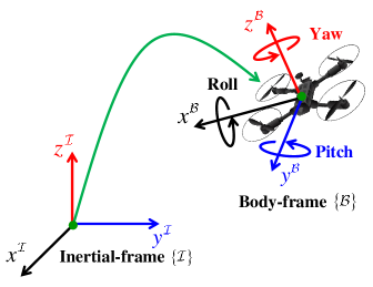
Figure 1: The relative orientation between body-frame and inertial-frame of a rigid-body in 3D space.

Let the superscripts $\mathcal{I}$ and $\mathcal{B}$ denote a vector associated with the inertial-frame and body-frame, respectively. Consider ${\rm v}_{i}^{\mathcal{I}}\in\mathbb{R}^{3}$ to be a known vector in the inertial-frame and to be measured in the coordinate system fixed to the rigid-body such that

$${\rm v}_{i}^{\mathcal{B}}=R^{\top}{\rm v}_{i}^{\mathcal{I}}+{\rm b}_{i}^{\mathcal{B}}+\omega_{i}^{\mathcal{B}}$$ (10)

where ${\rm v}_{i}^{\mathcal{B}}\in\mathbb{R}^{3}$ is the $i$th body-frame measurement associated with ${\rm v}_{i}^{\mathcal{I}}$. ${\rm b}_{i}^{\mathcal{B}}\in\mathbb{R}^{3}$ stands for the bias component, and $\omega_{i}^{\mathcal{B}}\in\mathbb{R}^{3}$ denotes the noise component attached to the $i$th body-frame measurement for $i=1,2,\ldots,n$. Suppose that the instantaneous set of size $n\geq 2$ consisting of known inertial-frame and measured body-frame vectors is non-collinear. Therefore, the attitude can be established. Moreover, two non-collinear vectors $\left(n=2\right)$ are generally sufficient for attitude reconstruction, e.g., [2, 15, 4, 16, 5, 27]. In case when $n=2$, the third inertial-frame and body-frame vectors can be obtained by the cross product such that ${\rm v}_{3}^{\mathcal{I}}={\rm v}_{1}^{\mathcal{I}}\times{\rm v}_{2}^{\mathcal{I}}$ and ${\rm v}_{3}^{\mathcal{B}}={\rm v}_{1}^{\mathcal{B}}\times{\rm v}_{2}^{\mathcal{B}}$, respectively. The inertial-frame and body-frame vectors can be normalized and their normalized values can be implemented in the estimation of the attitude in the following manner

$$\upsilon_{i}^{\mathcal{I}}=\frac{{\rm v}_{i}^{\mathcal{I}}}{||{\rm v}_{i}^{\mathcal{I}}||},\hskip 10.00002pt\upsilon_{i}^{\mathcal{B}}=\frac{{\rm v}_{i}^{\mathcal{B}}}{||{\rm v}_{i}^{\mathcal{B}}||}$$ (11)

Hence, the attitude can be obtained knowing $\upsilon_{i}^{\mathcal{I}}$ and $\upsilon_{i}^{\mathcal{B}}$. For simplicity, it is considered that the body frame vector (${\rm v}_{i}^{\mathcal{B}}$) is noise and bias free in the stability analysis. The Simulation Section, on the other hand, takes noise and bias associated with the measurements into account. The angular velocity of the moving body relative to the inertial-frame is measured by the rate gyros as

$$\Omega_{m}=\Omega+b+\omega$$ (12)

where $\Omega\in\mathbb{R}^{3}$ is the true value of angular velocity and $b$ and $\omega$ denote the bias and noise components, respectively, attached to the measurement of angular velocity for all $b,\omega\in\mathbb{R}^{3}$. The kinematics of the true attitude are described by

$$\dot{R}=R\left[\Omega\right]_{\times}$$ (13)

where $\Omega\in\left\{\mathcal{B}\right\}$. Considering the normalized Euclidean distance of $R$ in (1) and the identity in (9), the kinematics of the true attitude in (13) can be defined in terms of normalized Euclidean distance as

$$\frac{d}{dt}||R||_{I} =-\frac{1}{4}{\rm Tr}\left\{\dot{R}\right\}$$

$$=-\frac{1}{4}{\rm Tr}\left\{\boldsymbol{\mathcal{P}}_{a}\left(R\right)\left[\Omega\right]_{\times}\right\}$$

$$=\frac{1}{2}\mathbf{vex}\left(\boldsymbol{\mathcal{P}}_{a}\left(R\right)\right)^{\top}\Omega$$ (14)

For the sake of simplicity, let us neglect the noise attached to angular velocity measurements such that the kinematics of the normalized Euclidean distance in (14) become

$$\frac{d}{dt}||R||_{I}=\frac{1}{2}\mathbf{vex}\left(\boldsymbol{\mathcal{P}}_{a}\left(R\right)\right)^{\top}\left(\Omega_{m}-b\right)$$ (15)

Now, we introduce Lemma 1 which is going to be applicable in the subsequent filter derivation.

Lemma 1.

Let $R\in\mathbb{SO}\left(3\right)$, $M^{\mathcal{B}}=\left(M^{\mathcal{B}}\right)^{\top}\in\mathbb{R}^{3\times 3}$, $M^{\mathcal{B}}$ be nonsingular, ${\rm Tr}\left\{M^{\mathcal{B}}\right\}=3$, and $\bar{\mathbf{M}}^{\mathcal{B}}={\rm Tr}\left\{M^{\mathcal{B}}\right\}\mathbf{I}_{3}-M^{\mathcal{B}}$, while the minimum singular value of $\bar{\mathbf{M}}^{\mathcal{B}}$ is $\underline{\lambda}:=\underline{\lambda}\left(\bar{\mathbf{M}}^{\mathcal{B}}\right)$. Then, the following holds:

$$||\mathbf{vex}\left(\boldsymbol{\mathcal{P}}_{a}\left(R\right)\right)||^{2}=4\left(1-||R||_{I}\right)||R||_{I}$$ (16)

$$\frac{2}{\underline{\lambda}}\frac{||\mathbf{vex}\left(\boldsymbol{\mathcal{P}}_{a}\left(M^{\mathcal{B}}R\right)\right)||^{2}}{1+{\rm Tr}\left\{\left(M^{\mathcal{B}}\right)^{-1}M^{\mathcal{B}}R\right\}} \geq\left\|M^{\mathcal{B}}R\right\|_{I}$$ (17)

Proof. See Appendix A.

III-B Estimator Structure and Error Criteria

The goal of attitude estimator in this work is to achieve accurate estimate of the true attitude satisfying transient as well as steady-state characteristics. In this subsection general framework of the nonlinear attitude filter on $\mathbb{SO}\left(3\right)$ is introduced. Next, the error dynamics are expressed with respect to normalized Euclidean distance. Let $\hat{R}$ denote the estimate of the true attitude $R$ and $\tilde{R}=R^{\top}\hat{R}$ denote the attitude error between body-frame and estimator-frame. Consider the following nonlinear attitude filter on $\mathbb{SO}\left(3\right)$

$$\dot{\hat{R}} =\hat{R}\left[\Omega_{m}-\hat{b}-W\right]_{\times},\quad\hat{R}\left(0\right)=\hat{R}_{0}$$ (18)

$$\dot{\hat{b}} =\frac{1}{2}\mathbf{K}_{b}\mathbf{vex}\left(\boldsymbol{\mathcal{P}}_{a}\left(\boldsymbol{\Phi}\right)\right),\quad\hat{b}\left(0\right)=\hat{b}_{0}$$ (19)

$$W =2\mathbf{K}_{W}\mathbf{vex}\left(\boldsymbol{\mathcal{P}}_{a}\left(\boldsymbol{\Phi}\right)\right)$$ (20)

with $\hat{b}$ being the estimate of the true rate-gyro bias $b$, $\mathbf{K}_{b}$ being a time-variant gain associated with $\hat{b}$, $\mathbf{K}_{W}$ being a time-variant gain associated with the correction factor $W$, and $\boldsymbol{\Phi}$ being a matrix associated with attitude error $\tilde{R}$. Define the unstable set $\mathcal{U}\subseteq\mathbb{SO}\left(3\right)$ by $\mathcal{U}:=\left\{\left.\tilde{R}_{0}\right|{\rm Tr}\left\{\tilde{R}_{0}\right\}=-1\right\}$ with $\tilde{R}_{0}=\tilde{R}\left(0\right)$. $\mathbf{K}_{b}$, $\mathbf{K}_{W}$, and $\boldsymbol{\Phi}$ will be defined subsequently. In particular, the dynamic gains $\mathbf{K}_{b}$ and $\mathbf{K}_{W}$ will be selected such that their values become increasingly aggressive as $\tilde{R}$ approaches the unstable equilibria ${\rm Tr}\left\{\tilde{R}_{0}\right\}\rightarrow-1$, and reduce significantly as $\tilde{R}$ approaches $\mathbf{I}_{3}$.

Remark 1.

In the conventional design of nonlinear attitude filters, for example [4, 5, 12, 14], $\mathbf{K}_{b}$ and $\mathbf{K}_{W}$ are selected as positive constant gains. However, the weakness of the conventional design of nonlinear attitude filters is that smaller values of $\mathbf{K}_{b}$ and $\mathbf{K}_{W}$ result in slower transient performance with less oscillatory behavior in the steady-state. In contrast, higher values of $\mathbf{K}_{b}$ and $\mathbf{K}_{W}$ generate faster transient performance with higher oscillation in the steady-state.

Consider the error between body-frame and estimator-frame being defined as

$$\tilde{R}=R^{\top}\hat{R}$$ (21)

Also, define the error in bias estimation by

$$\tilde{b} =b-\hat{b}$$ (22)

From (13) and (18) the error dynamics can be found to be

$$\dot{\tilde{R}} =R^{\top}\hat{R}\left[\Omega_{m}-\hat{b}-W\right]_{\times}-\left[\Omega\right]_{\times}R^{\top}\hat{R}$$

$$=\tilde{R}\left[\tilde{b}-W\right]_{\times}+\tilde{R}\left[\Omega\right]_{\times}-\left[\Omega\right]_{\times}\tilde{R}$$ (23)

Considering (13) and (14), the error dynamics in (23) are represented with regards to normalized Euclidean distance

$$\frac{d}{dt}||\tilde{R}||_{I} =\frac{d}{dt}\frac{1}{4}{\rm Tr}\left\{\mathbf{I}_{3}-\tilde{R}\right\}$$

$$=-\frac{1}{4}{\rm Tr}\left\{\tilde{R}\left[\tilde{b}-W\right]_{\times}\right\}-\frac{1}{4}{\rm Tr}\left\{\left[\tilde{R},\left[\Omega\right]_{\times}\right]\right\}$$

$$=\frac{1}{2}\mathbf{vex}\left(\boldsymbol{\mathcal{P}}_{a}\left(\tilde{R}\right)\right)^{\top}\left(\tilde{b}-W\right)$$ (24)

where ${\rm Tr}\left\{\tilde{R}\left[\tilde{b}\right]_{\times}\right\}=-2\mathbf{vex}\left(\boldsymbol{\mathcal{P}}_{a}\left(\tilde{R}\right)\right)^{\top}\tilde{b}$ as given in (9) and ${\rm Tr}\left\{\left[\tilde{R},\left[\Omega\right]_{\times}\right]\right\}=0$ as defined in (7).

III-C Prescribed Performance

This subsection aims to reformulate the problem such that the normalized Euclidean distance of the attitude error $||\tilde{R}\left(t\right)||_{I}$ satisfies the predefined transient as well as steady-state measures set by the user. Initially, the error $||\tilde{R}\left(t\right)||_{I}$ is contained within a predefined large set and decreases systematically and smoothly to a predefined narrow set through a prescribed performance function (PPF) [20]. This is accomplished by first defining a configuration error function [20, 23, 24]. Let $\xi\left(t\right)$ be a positive smooth and time-decreasing performance function such that $\xi:\mathbb{R}_{+}\to\mathbb{R}_{+}$ and $\lim\limits_{t\to\infty}\xi\left(t\right)=\xi_{\infty}>0$. The general expression of the PPF is as follows

$$\xi\left(t\right)=\left(\xi_{0}-\xi_{\infty}\right)\exp\left(-\ell t\right)+\xi_{\infty}$$ (25)

where $\xi_{0}=\xi\left(0\right)$ is the upper bound of the predefined large set, also known to be the initial value of the PPF, $\xi_{\infty}$ is the upper bound of the small set such that the steady-state error is confined by $\pm\xi_{\infty}$, while $\ell$ is a positive constant controlling the convergence rate of the set boundaries $\xi\left(t\right)$ with respect to time from $\xi_{0}$ to $\xi_{\infty}$. It is sufficient to force $||\tilde{R}\left(t\right)||_{I}$ to obey a predefined transient and steady-state characteristics, if the following conditions are met:

$$-\delta\xi\left(t\right)<||\tilde{R}\left(t\right)||_{I}<\xi\left(t\right), \text{ if }||\tilde{R}\left(0\right)||_{I}\geq 0,\forall t\geq 0$$ (26)

$$-\xi\left(t\right)<||\tilde{R}\left(t\right)||_{I}<\delta\xi\left(t\right), \text{ if }||\tilde{R}\left(0\right)||_{I}<0,\forall t\geq 0$$ (27)

where $\delta$ is selected such that $1\geq\delta\geq 0$. The tracking error $||\tilde{R}\left(t\right)||_{I}$, with PPF decreasing systematically from a known large set to a known small set in accordance with (26) and (27) is illustrated in Figure 2.

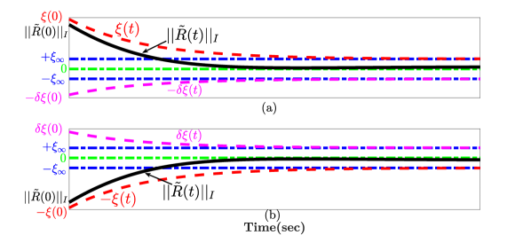
Figure 2: A detailed representation of tracking normalized Euclidean distance error $||\tilde{R}\left(t\right)||_{I}$ with PPF satisfying (a) Eq. (26); (b) Eq. (27).

Remark 2.

As explained in [20, 23], knowing the sign of $||\tilde{R}\left(0\right)||_{I}$ is sufficient to satisfy the performance constraints and maintain the error convergence within the predefined dynamically decreasing boundaries for all $t>0$. Since $||\tilde{R}\left(0\right)||_{I}\in\left[0,1\right]$, $||\tilde{R}\left(0\right)||_{I}$ is guaranteed to be greater than or equal to 0 for any attitude initialization, and therefore the only possible condition is (26). If the condition in (26) is met, the maximum steady-state error will be less than $\xi_{\infty}$, the maximum overshoot will be less than $-\delta\xi\left(0\right)$, and $||\tilde{R}\left(t\right)||_{I}$ will be confined between $\xi\left(t\right)$ and $\delta\xi\left(t\right)$ as given in the upper portion of Figure 2.

Let us define

$$||\tilde{R}\left(t\right)||_{I}=\xi\left(t\right)\mathcal{Z}\left(\mathcal{E}\right)$$ (28)

with $\xi\left(t\right)\in\mathbb{R}$ being given in (25), $\mathcal{E}\in\mathbb{R}$ being a transformed error, and $\mathcal{Z}\left(\mathcal{E}\right)$ being a smooth function which satisfies Assumption 1:

Assumption 1.

The smooth function $\mathcal{Z}\left(\mathcal{E}\right)$ must satisfy [20]:

1. $\mathcal{Z}\left(\mathcal{E}\right)$ is smooth and strictly increasing.

2. $\mathcal{Z}\left(\mathcal{E}\right)$ is bounded between two predefined bounds
   $-\underline{\delta}<\mathcal{Z}\left(\mathcal{E}\right)<\bar{\delta},{\rm\text{for}}||\tilde{R}\left(0\right)||_{I}\geq 0$
   with $\bar{\delta}$ and $\underline{\delta}$ being positive constants and $\underline{\delta}\leq\bar{\delta}$.

3. $\underset{\mathcal{E}\rightarrow-\infty}{\lim}\mathcal{Z}\left(\mathcal{E}\right)=-\underline{\delta}$ and $\underset{\mathcal{E}\rightarrow+\infty}{\lim}\mathcal{Z}\left(\mathcal{E}\right)=\bar{\delta}$ where

   $$\mathcal{Z}\left(\mathcal{E}\right)=\frac{\bar{\delta}\exp\left(\mathcal{E}\right)-\underline{\delta}\exp\left(-\mathcal{E}\right)}{\exp\left(\mathcal{E}\right)+\exp\left(-\mathcal{E}\right)}$$ (29)

One could find the transformed error to be

$$\mathcal{E}\left(||\tilde{R}\left(t\right)||_{I},\xi\left(t\right)\right)=\mathcal{Z}^{-1}\left(\frac{||\tilde{R}\left(t\right)||_{I}}{\xi\left(t\right)}\right)$$ (30)

where $\mathcal{E}\in\mathbb{R}$, $\mathcal{Z}\in\mathbb{R}$ and $\mathcal{Z}^{-1}\in\mathbb{R}$ are smooth functions. For clarity, let $\xi:=\xi\left(t\right)$, $||\tilde{R}||_{I}:=||\tilde{R}\left(t\right)||_{I}$ and $\mathcal{E}:=\mathcal{E}\left(\cdot,\cdot\right)$. The transformed error $\mathcal{E}$ plays a prominent role driving the error dynamics from constrained form in either (26) or (27) to that in (30) which is unconstrained. One can find from (29) that the transformed error is

$$\mathcal{E}= \frac{1}{2}\text{ln}\frac{\underline{\delta}+||\tilde{R}||_{I}/\xi}{\bar{\delta}-||\tilde{R}||_{I}/\xi}$$ (31)

Remark 3.

[20, 23] Consider the transformed error in (31). If $\mathcal{E}\left(t\right)$ is guaranteed to be bounded for all $t\geq 0$, the performance function $\xi\left(t\right)$ can be used to bound the transient and steady-state of the tracking error ($||\tilde{R}||_{I}$) allowing it to achieve the prescribed performance.

Proposition 1.

Consider the normalized Euclidean distance error $||\tilde{R}||_{I}$ being defined by (1) and from (28), (29), (30) let the transformed error be given as in (31) with $\underline{\delta}=\bar{\delta}$. Then the following statements hold.

1. The transformed error $\mathcal{E}>0\forall||\tilde{R}||_{I}\neq 0$ and $\mathcal{E}=0$ only at $||\tilde{R}||_{I}=0$.

2. The critical point of $\mathcal{E}$ satisfies $||\tilde{R}||_{I}=0$.

3. The only critical point of $\mathcal{E}$ is $\tilde{R}=\mathbf{I}_{3}$.

Proof. Letting $\underline{\delta}=\bar{\delta}$ with the prescribed performance constraints $||\tilde{R}||_{I}\leq\xi$, the expression $\left(\underline{\delta}+||\tilde{R}||_{I}/\xi\right)/\left(\bar{\delta}-||\tilde{R}||_{I}/\xi\right)$ in (31) is always greater than or equal to 1. Accordingly, $\mathcal{E}>0\forall||\tilde{R}||_{I}\neq 0$ and $\mathcal{E}=0$ at $||\tilde{R}||_{I}=0$ which proves (i). For (ii) and (iii), from (1), $||\tilde{R}||_{I}=0$ if and only if $\tilde{R}=\mathbf{I}_{3}$. Thus, the critical point of $\mathcal{E}$ satisfies $\tilde{R}=\mathbf{I}_{3}$ and, consequently, also satisfies $||\tilde{R}||_{I}=0$ which proves (ii) and (iii). Let us define a new variable $\mu:=\mu\left(||\tilde{R}||_{I},\xi\right)$ such that

$$\begin{split}\mu&=\frac{1}{2\xi}\frac{\partial\mathcal{Z}^{-1}\left(||\tilde{R}||_{I}/\xi\right)}{\partial\left(||\tilde{R}||_{I}/\xi\right)}\\ &=\frac{1}{2\xi}\left(\frac{1}{\underline{\delta}+||\tilde{R}||_{I}/\xi}+\frac{1}{\bar{\delta}-||\tilde{R}||_{I}/\xi}\right)\end{split}$$ (32)

Consequently, the derivative of the transformed error is governed by

$$\dot{\mathcal{E}} =\frac{1}{2\xi}\left(\frac{1}{\underline{\delta}+||\tilde{R}||_{I}/\xi}+\frac{1}{\bar{\delta}-||\tilde{R}||_{I}/\xi}\right)\left(\frac{d}{dt}||\tilde{R}||_{I}-\frac{\dot{\xi}}{\xi}||\tilde{R}||_{I}\right)$$

$$=\mu\left(\frac{1}{2}\mathbf{vex}\left(\boldsymbol{\mathcal{P}}_{a}\left(\tilde{R}\right)\right)^{\top}\left(\tilde{b}-W\right)-\frac{\dot{\xi}}{\xi}||\tilde{R}||_{I}\right)$$ (33)

with direct substitution of (24) in (33). Next section presents two nonlinear attitude filters on $\mathbb{SO}\left(3\right)$ with prescribed performance which guarantees $\mathcal{E}\in\mathcal{L}_{\infty},\forall t\geq 0$ and, thus, satisfies (26) provided that $0\leq||\tilde{R}\left(0\right)||_{I}<\xi\left(0\right)$.

IV Nonlinear Complementary Filters On $\mathbb{SO}\left(3\right)$ with Prescribed Performance

The primary objective of this section is to propose two nonlinear attitude estimators on $\mathbb{SO}\left(3\right)$ with normalized Euclidean distance error satisfying a predefined transient as well as steady-state performance given by the user. The constrained error $||\tilde{R}||_{I}$ is relaxed to unconstrained $\mathcal{E}$. The first filter is termed a semi-direct attitude filter with prescribed performance because it requires the attitude to be reconstructed via the set of vectorial measurements as defined in (11), in addition to the measurement of the angular velocity in (12). The second filter is called a direct attitude filter with prescribed performance because it uses the vectorial measurements in (11) and the angular velocity measurement in (12) directly without the need for attitude reconstruction.

IV-A Semi-direct Attitude Filter with Prescribed Performance

Let $R_{y}$ denote the reconstructed attitude of $R$. There are many methods to reconstruct $R_{y}$, for instance, TRIAD [1], QUEST [2], or SVD [3]. Consider the following filter kinematics

$$\dot{\hat{R}} =\hat{R}\left[\Omega_{m}-\hat{b}-W\right]_{\times},\quad\hat{R}\left(0\right)=\hat{R}_{0}$$ (34)

$$\dot{\hat{b}} =\frac{1}{2}\gamma\mu\mathcal{E}\mathbf{vex}\left(\boldsymbol{\mathcal{P}}_{a}\left(\tilde{R}\right)\right),\quad\hat{b}\left(0\right)=\hat{b}_{0},\tilde{R}=R_{y}^{\top}\hat{R}$$ (35)

$$W =2\frac{k_{w}\mu\mathcal{E}-\dot{\xi}/4\xi}{1-||\tilde{R}||_{I}}\mathbf{vex}\left(\boldsymbol{\mathcal{P}}_{a}\left(\tilde{R}\right)\right),\hskip 10.00002pt\tilde{R}=R_{y}^{\top}\hat{R}$$ (36)

with $\mathcal{E}$ and $\mu$ being defined in (31) and (32), respectively, $k_{w}$ and $\gamma$ being positive constants, $||\tilde{R}||_{I}=\frac{1}{4}{\rm Tr}\left\{\mathbf{I}_{3}-\tilde{R}\right\}$ being defined in (1), $\xi$ being PPF defined in (25), and $\hat{b}$ being the estimate of $b$.

Theorem 1.

Consider the rotation kinematics in (13), measurements of angular velocity in (12) with no noise associated with the measurement $\Omega_{m}=\Omega+b$, in addition to other vector measurements given in (10) coupled with the filter in (34), (35) and (36). Suppose that measurements can be made on two or more body-frame non-collinear vectors. Define $\mathcal{U}\subseteq\mathbb{SO}\left(3\right)\times\mathbb{R}^{3}$ by $\mathcal{U}:=\left\{\left.\left(\tilde{R}_{0},\tilde{b}_{0}\right)\right|{\rm Tr}\left\{\tilde{R}_{0}\right\}=-1,\tilde{b}_{0}=\underline{\boldsymbol{0}}_{3}\right\}$ with $\tilde{R}_{0}=\tilde{R}\left(0\right)$ and $\tilde{b}_{0}=\tilde{b}\left(0\right)$. For almost any initial condition such that $\tilde{R}_{0}\notin\mathcal{U}$ and $\mathcal{E}\left(0\right)\in\mathcal{L}_{\infty}$, then, all signals in the closed loop are bounded, $\lim_{t\rightarrow\infty}\mathcal{E}\left(t\right)=0$ and $\tilde{R}$ asymptotically approaches $\mathbf{I}_{3}$.

Theorem 1 guarantees that the observer dynamics in (34), (35) and (36) are stable with $\mathcal{E}\left(t\right)$ approaching asymptotically the origin. Since, $\mathcal{E}\left(t\right)$ is bounded, $||\tilde{R}||_{I}$ obeys the prescribed transient and steady-state performance introduced in (25).

Proof. Let the error in attitude and bias be defined by $\tilde{R}=R^{\top}\hat{R}$ and $\tilde{b}=b-\hat{b}$ similar to (21) and (22), respectively. From (13) and (34), the error dynamics can be obtained as in (23). Also, in view of (13) and (14), the error dynamics are analogous to (24) in terms of normalized Euclidean distance. Therefore, considering (14) and (33), the derivative of the transformed error can be found to be

$$\dot{\mathcal{E}}= \mu\left(\frac{1}{2}\mathbf{vex}\left(\boldsymbol{\mathcal{P}}_{a}\left(\tilde{R}\right)\right)^{\top}\left(\tilde{b}-W\right)-\frac{\dot{\xi}}{\xi}||\tilde{R}||_{I}\right)$$ (37)

Consider the following candidate Lyapunov function

$$V\left(\mathcal{E},\tilde{b}\right) =\frac{1}{2}\mathcal{E}^{2}+\frac{1}{2\gamma}||\tilde{b}||^{2}$$ (38)

Differentiating $V$ in (38) and substituting for $\dot{\hat{b}}$ and $W$ in (35), and (36), respectively, one obtains

$$\dot{V}= \mathcal{E}\dot{\mathcal{E}}-\frac{1}{\gamma}\tilde{b}^{\top}\dot{\hat{b}}$$

$$= \mu\mathcal{E}\left(\frac{1}{2}\mathbf{vex}\left(\boldsymbol{\mathcal{P}}_{a}\left(\tilde{R}\right)\right)^{\top}\left(\tilde{b}-W\right)-\frac{\dot{\xi}}{\xi}||\tilde{R}||_{I}\right)-\frac{1}{\gamma}\tilde{b}^{\top}\dot{\hat{b}}$$

$$= -\mathcal{E}\mu\left(\frac{k_{w}\mu\mathcal{E}-\dot{\xi}/4\xi}{1-||\tilde{R}||_{I}}\left\|\mathbf{vex}\left(\boldsymbol{\mathcal{P}}_{a}\left(\tilde{R}\right)\right)\right\|^{2}+\frac{\dot{\xi}}{\xi}||\tilde{R}||_{I}\right)$$ (39)

Substituting for $\left\|\mathbf{vex}\left(\boldsymbol{\mathcal{P}}_{a}\left(\tilde{R}\right)\right)\right\|^{2}=4\left(1-||\tilde{R}||_{I}\right)||\tilde{R}||_{I}$ as defined in (16), the expression in (39) becomes

$$\dot{V}= -4k_{w}||\tilde{R}||_{I}\mu^{2}\mathcal{E}^{2}$$ (40)

This implies that $V\left(t\right)\leq V\left(0\right),\forall t\geq 0$. Given $\tilde{R}_{0}\notin\mathcal{U}$ implies that $\tilde{b}$ remains bounded for all $t\geq 0$, and, therefore, $\mathcal{E}$ is bounded and well defined for all $t\geq 0$. It can be shown that

$$\ddot{V}= -4k_{w}\left(2\left(\mathcal{E}\dot{\mathcal{E}}\mu^{2}+\mathcal{E}^{2}\mu\dot{\mu}\right)||\tilde{R}||_{I}+\mathcal{E}^{2}\mu^{2}||\dot{\tilde{R}}||_{I}\right)$$ (41)

From (32), it can be found that

$$\dot{\mu}=-\frac{1}{2}\frac{\underline{\delta}\dot{\xi}+||\dot{\tilde{R}}||_{I}}{\left(\underline{\delta}\xi+||\tilde{R}||_{I}\right)^{2}}-\frac{1}{2}\frac{\bar{\delta}\dot{\xi}-||\dot{\tilde{R}}||_{I}}{\left(\bar{\delta}\xi-||\tilde{R}||_{I}\right)^{2}}$$ (42)

where $\dot{\xi}=-\ell\left(\xi^{0}-\xi^{\infty}\right)\exp\left(-\ell t\right)$. Since $||\dot{\tilde{R}}||_{I}$ is bounded, $\dot{\mu}$ is bounded which shows that $\ddot{V}$ is bounded for all $t\geq 0$. Consequently, $\dot{V}$ is uniformly continuous, and according to Barbalat Lemma, $\dot{V}\rightarrow 0$ indicates that one or more of the following conditions are true

1. $||\mathcal{E}||\rightarrow 0$.

2. $||\tilde{R}||_{I}\rightarrow 0$.

3. $||\mathcal{E}||\rightarrow 0$ and $||\tilde{R}||_{I}\rightarrow 0$.

as $t\rightarrow\infty$. According to property (i) and (ii) of Proposition 1, $||\mathcal{E}||\rightarrow 0$ means $||\tilde{R}||_{I}\rightarrow 0$ and vice versa. Therefore, $\dot{V}\rightarrow 0$ as $t\rightarrow\infty$ strictly indicates that $||\mathcal{E}||\rightarrow 0$ and $||\tilde{R}||_{I}\rightarrow 0$. As stated by property (iii) of Proposition 1, $||\mathcal{E}||\rightarrow 0$ implies that $\tilde{R}$ asymptotically approaches $\mathbf{I}_{3}$. Hence, $\dot{V}\rightarrow 0$ means that $\tilde{R}$ asymptotically approaches $\mathbf{I}_{3}$, which completes the proof.

IV-B Direct Attitude Filter with Prescribed Performance

Let $R_{y}$ denote the reconstructed attitude of $R$ obtained through a set of vectorial measurements in (11). Although there are many methods to reconstruct $R_{y}$, this may add computational cost. The filter proposed in the previous Subsection IV-A requires $R_{y}$ to obtain the attitude error $\tilde{R}=R_{y}^{\top}\hat{R}$, for example (the Appendix in [15, 27]). In this Subsection the aforementioned weakness is eliminated by proposing a nonlinear filter with prescribed performance in terms of direct measurements from the inertial and body-frame units. Let us recall $\upsilon_{i}^{\mathcal{I}}\in\left\{\mathcal{I}\right\}$ and $\upsilon_{i}^{\mathcal{B}}\in\left\{\mathcal{B}\right\}$ from (10) and (11) for $i=1,\ldots,n$. Let us define

$$M^{\mathcal{I}} =\left(M^{\mathcal{I}}\right)^{\top}=\sum_{i=1}^{n}s_{i}\upsilon_{i}^{\mathcal{I}}\left(\upsilon_{i}^{\mathcal{I}}\right)^{\top}$$

$$M^{\mathcal{B}} =\left(M^{\mathcal{B}}\right)^{\top}=\sum_{i=1}^{n}s_{i}\upsilon_{i}^{\mathcal{B}}\left(\upsilon_{i}^{\mathcal{B}}\right)^{\top}$$

$$=R^{\top}M^{\mathcal{I}}R$$ (43)

where $s_{i}>0$ refers to confidence level of the $i$th sensor measurements, and in this work $s_{i}$ is selected such that $\sum_{i=1}^{n}s_{i}=3$. According to (43), $M^{\mathcal{I}}$ and $M^{\mathcal{B}}$ are symmetric matrices. Assume that at least two non-collinear inertial-frame and measured body-frame vectors are available. If two typical vectors are available for measurements, $n=2$, the third vector is obtained by the cross product as mentioned in Subsection III-A. Thereby, the set of vectors is non-collinear and $M^{\mathcal{B}}$ is nonsingular with ${\rm rank}\left(M^{\mathcal{B}}\right)=3$. Hence, the three eigenvalues of $M^{\mathcal{B}}$ are greater than zero. Let $\bar{\mathbf{M}}^{\mathcal{B}}={\rm Tr}\left\{M^{\mathcal{B}}\right\}\mathbf{I}_{3}-M^{\mathcal{B}}\in\mathbb{R}^{3\times 3}$, provided that ${\rm rank}\left(M^{\mathcal{B}}\right)=3$, then, the following three statements hold ([28] page. 553):

1. $\bar{\mathbf{M}}^{\mathcal{B}}$ is a symmetric and positive-definite matrix.

2. The eigenvectors of $M^{\mathcal{B}}$ coincide with the eigenvectors of $\bar{\mathbf{M}}^{\mathcal{B}}$.

3. Define the three eigenvalues of $M^{\mathcal{B}}$ by $\lambda\left(M^{\mathcal{B}}\right)=\left\{\lambda_{1},\lambda_{2},\lambda_{3}\right\}$, then $\lambda\left(\bar{\mathbf{M}}^{\mathcal{B}}\right)=\{\lambda_{3}+\lambda_{2},\lambda_{3}+\lambda_{1},\lambda_{2}+\lambda_{1}\}$ such that the minimum singular value $\underline{\lambda}\left(\bar{\mathbf{M}}^{\mathcal{B}}\right)>0$.

In the remainder of this section, we assume that ${\rm rank}\left(M^{\mathcal{B}}\right)=3$, and accordingly the three above-mentioned statements are true. Define

$$\hat{\upsilon}_{i}^{\mathcal{B}}=\hat{R}^{\top}\upsilon_{i}^{\mathcal{I}}$$ (44)

Define the error in attitude and bias by $\tilde{R}=R^{\top}\hat{R}$ and $\tilde{b}=b-\hat{b}$ which is similar to (21) and (22), respectively. In order to derive the explicit filter, it is necessary to present the following equations expressed in terms of vector measurements. From identity (3), one can find

$$\left[\sum_{i=1}^{n}\frac{s_{i}}{2}\hat{\upsilon}_{i}^{\mathcal{B}}\times\upsilon_{i}^{\mathcal{B}}\right]_{\times} =\sum_{i=1}^{n}\frac{s_{i}}{2}\left(\upsilon_{i}^{\mathcal{B}}\left(\hat{\upsilon}_{i}^{\mathcal{B}}\right)^{\top}-\hat{\upsilon}_{i}^{\mathcal{B}}\left(\upsilon_{i}^{\mathcal{B}}\right)^{\top}\right)$$

$$=\frac{1}{2}R^{\top}M^{\mathcal{I}}R\tilde{R}-\frac{1}{2}\tilde{R}^{\top}R^{\top}M^{\mathcal{I}}R$$

$$=\boldsymbol{\mathcal{P}}_{a}\left(M^{\mathcal{B}}\tilde{R}\right)$$

such that

$$\mathbf{vex}\left(\boldsymbol{\mathcal{P}}_{a}\left(M^{\mathcal{B}}\tilde{R}\right)\right)=\sum_{i=1}^{n}\frac{s_{i}}{2}\hat{\upsilon}_{i}^{\mathcal{B}}\times\upsilon_{i}^{\mathcal{B}}$$ (45)

The normalized Euclidean distance of $M^{\mathcal{B}}\tilde{R}$ can be found to be

$$||M^{\mathcal{B}}\tilde{R}||_{I} =\frac{1}{4}{\rm Tr}\left\{\mathbf{I}_{3}-M^{\mathcal{B}}\tilde{R}\right\}$$

$$=\frac{1}{4}{\rm Tr}\left\{\mathbf{I}_{3}-\sum_{i=1}^{n}s_{i}\upsilon_{i}^{\mathcal{B}}\left(\hat{\upsilon}_{i}^{\mathcal{B}}\right)^{\top}\right\}$$

$$=\frac{1}{4}\sum_{i=1}^{n}s_{i}\left(1-\left(\hat{\upsilon}_{i}^{\mathcal{B}}\right)^{\top}\upsilon_{i}^{\mathcal{B}}\right)$$ (46)

Let us introduce the following variable

$$\boldsymbol{\Upsilon}\left(M^{\mathcal{B}},\tilde{R}\right)$$

$$\hskip 20.00003pt={\rm Tr}\left\{\left(M^{\mathcal{B}}\right)^{-1}M^{\mathcal{B}}\tilde{R}\right\}$$

$$\hskip 20.00003pt={\rm Tr}\left\{\left(\sum_{i=1}^{n}s_{i}\upsilon_{i}^{\mathcal{B}}\left(\upsilon_{i}^{\mathcal{B}}\right)^{\top}\right)^{-1}\sum_{i=1}^{n}s_{i}\upsilon_{i}^{\mathcal{B}}\left(\hat{\upsilon}_{i}^{\mathcal{B}}\right)^{\top}\right\}$$ (47)

Consequently, any $\mathbf{vex}\left(\boldsymbol{\mathcal{P}}_{a}\left(M^{\mathcal{B}}\tilde{R}\right)\right)$, $||M^{\mathcal{B}}\tilde{R}||_{I}$ and $\boldsymbol{\Upsilon}\left(M^{\mathcal{B}},\tilde{R}\right)$ will be obtained via a set of vectorial measurements as given in (45), (46), and (47), respectively, in all the subsequent calculations and derivations. Let us define the minimum singular value of $\bar{\mathbf{M}}^{\mathcal{B}}$ as $\underline{\lambda}:=\underline{\lambda}\left(\bar{\mathbf{M}}^{\mathcal{B}}\right)$, $\mathcal{E}:=\mathcal{E}\left(||M^{\mathcal{B}}\tilde{R}||_{I},\xi\right)$, and $\mu:=\mu\left(||M^{\mathcal{B}}\tilde{R}||_{I},\xi\right)$, and consider the following filter kinematics

$$\dot{\hat{R}}= \hat{R}\left[\Omega_{m}-\hat{b}-W\right]_{\times},\quad\hat{R}\left(0\right)=\hat{R}_{0}$$ (48)

$$\dot{\hat{b}}= \frac{1}{2}\gamma\mu\mathcal{E}\mathbf{vex}\left(\boldsymbol{\mathcal{P}}_{a}\left(M^{\mathcal{B}}\tilde{R}\right)\right),\quad\hat{b}\left(0\right)=\hat{b}_{0}$$ (49)

$$W= \frac{4}{\underline{\lambda}}\frac{k_{w}\mu\mathcal{E}-\dot{\xi}/\xi}{1+\boldsymbol{\Upsilon}\left(M^{\mathcal{B}},\tilde{R}\right)}\mathbf{vex}\left(\boldsymbol{\mathcal{P}}_{a}\left(M^{\mathcal{B}}\tilde{R}\right)\right)$$ (50)

where $\boldsymbol{\Upsilon}\left(M^{\mathcal{B}},\tilde{R}\right)$ and $\mathbf{vex}\left(\boldsymbol{\mathcal{P}}_{a}\left(M^{\mathcal{B}}\tilde{R}\right)\right)$ are defined in terms of vectorial measurements in (47) and (45), respectively, $\xi$ is a PPF defined in (25), $\mathcal{E}$ and $\mu$ are defined in (31) and (32), respectively, with every $||\tilde{R}||_{I}$ being replaced by $||M^{\mathcal{B}}\tilde{R}||_{I}$, $k_{w}$ and $\gamma$ are positive constants, and $\hat{b}$ is the estimate of $b$.

Theorem 2.

Consider the filter in (48), (49) and (50) to be coupled with the normalized vector measurements in (11) and angular velocity measurements in (12) with the assumption that no noise is associated with the measurement $\Omega_{m}=\Omega+b$. Let two or more body-frame non-collinear vectors be available for measurements such that $M^{\mathcal{B}}$ is nonsingular. Define $\mathcal{U}\subseteq\mathbb{SO}\left(3\right)\times\mathbb{R}^{3}$ by $\mathcal{U}:=\left\{\left.\left(\tilde{R}_{0},\tilde{b}_{0}\right)\right|{\rm Tr}\left\{\tilde{R}_{0}\right\}=-1,\tilde{b}_{0}=\underline{\boldsymbol{0}}_{3}\right\}$ with $\tilde{R}_{0}=\tilde{R}\left(0\right)$ and $\tilde{b}_{0}=\tilde{b}\left(0\right)$. If $\tilde{R}_{0}\notin\mathcal{U}$ and $\mathcal{E}\left(0\right)\in\mathcal{L}_{\infty}$, then, all error signals are bounded, while $\mathcal{E}\left(t\right)$ asymptotically approaches $0$ and $\tilde{R}$ asymptotically approaches $\mathbf{I}_{3}$.

The observer dynamics in (48), (49) and (50) are guaranteed by Theorem 2 to be stable as $\mathcal{E}\left(t\right)$ approaches the origin asymptotically. It follows that $\mathcal{E}\left(t\right)$ is bounded, which in turn causes $||\tilde{R}||_{I}$ to obey the prescribed transient and steady-state performance as described in (25) in consistence with Remark 3.

Proof. Consider the error in attitude and bias being defined similar to (21) and (22), respectively. From (13) and (34), the error dynamics can be found to be analogous to (23). From (43), one can find the derivative of $M^{\mathcal{B}}$ to be

$$\dot{M}^{\mathcal{B}} =\dot{R}^{\top}M^{\mathcal{I}}R+R^{\top}M^{\mathcal{I}}\dot{R}$$

$$=-\left[\Omega\right]_{\times}R^{\top}M^{\mathcal{I}}R+R^{\top}M^{\mathcal{I}}R\left[\Omega\right]_{\times}$$

$$=-\left[\Omega\right]_{\times}M^{\mathcal{B}}+M^{\mathcal{B}}\left[\Omega\right]_{\times}$$ (51)

Therefore, from (23) and (51), the derivative of $||M^{\mathcal{B}}\tilde{R}||_{I}$ can be expressed as

$$\frac{d}{dt}||M^{\mathcal{B}}\tilde{R}||_{I}= -\frac{1}{4}{\rm Tr}\left\{M^{\mathcal{B}}\dot{\tilde{R}}+\dot{M}^{\mathcal{B}}\tilde{R}\right\}$$

$$= -\frac{1}{4}{\rm Tr}\left\{M^{\mathcal{B}}\left(\left[\tilde{R},\left[\Omega\right]_{\times}\right]+\tilde{R}\left[\tilde{b}-W\right]_{\times}\right)\right\}$$

$$-\frac{1}{4}{\rm Tr}\left\{\left(-\left[\Omega\right]_{\times}M^{\mathcal{B}}+M^{\mathcal{B}}\left[\Omega\right]_{\times}\right)\tilde{R}\right\}$$

$$= -\frac{1}{4}{\rm Tr}\left\{M^{\mathcal{B}}\tilde{R}\left[\tilde{b}-W\right]_{\times}\right\}$$

$$-\frac{1}{4}{\rm Tr}\left\{\left[M^{\mathcal{B}}\tilde{R},\left[\Omega\right]_{\times}\right]\right\}$$

$$= \frac{1}{2}\mathbf{vex}\left(\boldsymbol{\mathcal{P}}_{a}\left(M^{\mathcal{B}}\tilde{R}\right)\right)^{\top}\left(\tilde{b}-W\right)$$ (52)

where ${\rm Tr}\left\{M^{\mathcal{B}}\tilde{R}\left[\tilde{b}\right]_{\times}\right\}=-2\mathbf{vex}\left(\boldsymbol{\mathcal{P}}_{a}\left(M^{\mathcal{B}}\tilde{R}\right)\right)^{\top}\tilde{b}$ as given in (9), and ${\rm Tr}\left\{\left[M^{\mathcal{B}}\tilde{R},\left[\Omega\right]_{\times}\right]\right\}=0$ as defined in (7). Thus, in view of (14) and (33), the derivative of the transformed error in the sense of (24) can be found to be

$$\dot{\mathcal{E}}= \frac{\mu}{2}\mathbf{vex}\left(\boldsymbol{\mathcal{P}}_{a}\left(M^{\mathcal{B}}\tilde{R}\right)\right)^{\top}\left(\tilde{b}-W\right)-\mu\frac{\dot{\xi}}{\xi}||M^{\mathcal{B}}\tilde{R}||_{I}$$ (53)

Define the following candidate Lyapunov function as

$$V\left(\mathcal{E},\tilde{b}\right) =\frac{1}{2}\mathcal{E}^{2}+\frac{1}{2\gamma}||\tilde{b}||^{2}$$ (54)

The derivative of $V:=V\left(\mathcal{E},\tilde{b}\right)$ in (54) can be expressed as

$$\dot{V}= \mathcal{E}\dot{\mathcal{E}}-\frac{1}{\gamma}\tilde{b}^{\top}\dot{\hat{b}}$$

$$= \mathcal{E}\mu\left(\frac{1}{2}\mathbf{vex}\left(\boldsymbol{\mathcal{P}}_{a}\left(M^{\mathcal{B}}\tilde{R}\right)\right)^{\top}\left(\tilde{b}-W\right)-\frac{\dot{\xi}}{\xi}||M^{\mathcal{B}}\tilde{R}||_{I}\right)$$

$$-\frac{1}{\gamma}\tilde{b}^{\top}\dot{\hat{b}}$$ (55)

Directly substituting for $\dot{\hat{b}}$ and $W$ in (49), and (50), respectively, one obtains

$$\dot{V}\leq \frac{\dot{\xi}}{\xi}\left(\frac{2}{\underline{\lambda}}\frac{\left\|\mathbf{vex}\left(\boldsymbol{\mathcal{P}}_{a}\left(M^{\mathcal{B}}\tilde{R}\right)\right)\right\|^{2}}{1+\boldsymbol{\Upsilon}\left(M^{\mathcal{B}},\tilde{R}\right)}-\left\|M^{\mathcal{B}}\tilde{R}\right\|_{I}\right)\mu\mathcal{E}$$

$$-\frac{2}{\underline{\lambda}}\frac{k_{w}\mu^{2}\mathcal{E}^{2}}{1+\boldsymbol{\Upsilon}\left(M^{\mathcal{B}},\tilde{R}\right)}\left\|\mathbf{vex}\left(\boldsymbol{\mathcal{P}}_{a}\left(M^{\mathcal{B}}\tilde{R}\right)\right)\right\|^{2}$$ (56)

One can also easily find

$$\frac{\dot{\xi}}{\xi}\left(\frac{2}{\underline{\lambda}}\frac{\left\|\mathbf{vex}\left(\boldsymbol{\mathcal{P}}_{a}\left(M^{\mathcal{B}}\tilde{R}\right)\right)\right\|^{2}}{1+\boldsymbol{\Upsilon}\left(M^{\mathcal{B}},\tilde{R}\right)}-\left\|M^{\mathcal{B}}\tilde{R}\right\|_{I}\right)\mu\mathcal{E}\leq 0$$ (57)

where $\mathcal{E}>0\forall||M^{\mathcal{B}}\tilde{R}||_{I}\neq 0$ and $\mathcal{E}=0$ at $||M^{\mathcal{B}}\tilde{R}||_{I}=0$ as given in (i) Proposition 1, and $\mu>0\forall t\geq 0$ as given in (32). Also, $\dot{\xi}$ is a negative strictly increasing component which satisfies $\dot{\xi}\rightarrow 0$ as $t\rightarrow\infty$, and $\xi:\mathbb{R}_{+}\to\mathbb{R}_{+}$ such that $\xi\rightarrow\xi_{\infty}$ as $t\rightarrow\infty$. Thus, $\dot{\xi}/\xi\leq 0$. In addition, consider (17) in Lemma 1, the expression in (57) is negative semi-definite. Consequently, the inequality in (56) can be expressed as

$$\dot{V}\leq -k_{w}\mu^{2}\mathcal{E}^{2}\left\|M^{\mathcal{B}}\tilde{R}\right\|_{I}$$ (58)

This implies that $V\left(t\right)\leq V\left(0\right),\forall t\geq 0$. Given that $\tilde{R}_{0}\notin\mathcal{U}$, $\tilde{b}$ is bounded for $t\geq 0$, and $\mathcal{E}\in\mathcal{L}_{\infty},\forall t\geq 0$. As such, $\mathcal{E}$ remains bounded and well-defined for all $t\geq 0$. In order to prove asymptotic convergence of $\mathcal{E}$ to the origin and $\tilde{R}$ to the identity for all $\tilde{R}_{0}\notin\mathcal{U}$, one obtains the second derivative of (54) as

$$\ddot{V}\leq -2k_{w}\left(\mathcal{E}\dot{\mathcal{E}}\mu^{2}+\mathcal{E}^{2}\mu\dot{\mu}\right)||M^{\mathcal{B}}\tilde{R}||_{I}$$

$$-k_{w}\mathcal{E}^{2}\mu^{2}\frac{d}{dt}||M^{\mathcal{B}}\tilde{R}||_{I}$$ (59)

Consider the result in (32), as such, it can be shown that

$$\dot{\mu}=-\frac{1}{2}\frac{\underline{\delta}\dot{\xi}+\frac{d}{dt}||M^{\mathcal{B}}\tilde{R}||_{I}}{\left(\underline{\delta}\xi+||\tilde{R}||_{I}\right)^{2}}-\frac{1}{2}\frac{\bar{\delta}\dot{\xi}-\frac{d}{dt}||M^{\mathcal{B}}\tilde{R}||_{I}}{\left(\bar{\delta}\xi-||\tilde{R}||_{I}\right)^{2}}$$ (60)

with $\dot{\xi}=-\ell\left(\xi^{0}-\xi^{\infty}\right)\exp\left(-\ell t\right)$. Due to the fact that $||\dot{\tilde{R}}||_{I}$ is bounded, $\dot{\mu}$ is bounded and in turn $\ddot{V}$ is bounded for all $t\geq 0$. Thus, $\dot{V}$ is uniformly continuous and in accordance with Barbalat Lemma, $\dot{V}\rightarrow 0$ implies that either $||\mathcal{E}||\rightarrow 0$ or $||M^{\mathcal{B}}\tilde{R}||_{I}\rightarrow 0$ or both $||\mathcal{E}||\rightarrow 0$ and $||M^{\mathcal{B}}\tilde{R}||_{I}\rightarrow 0$ as $t\rightarrow\infty$. From property (i) and (ii) of Proposition 1, $||\mathcal{E}||\rightarrow 0$ indicates that $||M^{\mathcal{B}}\tilde{R}||_{I}\rightarrow 0$ and vice versa. Thus, $\dot{V}\rightarrow 0$ implies that $||\mathcal{E}||\rightarrow 0$ and $||M^{\mathcal{B}}\tilde{R}||_{I}\rightarrow 0$, which means that $\tilde{R}$ asymptotically approaches $\mathbf{I}_{3}$ consistent with property (iii) of Proposition 1, which completes the proof.

It is clear that the gains associated with the vex operator of $\dot{\hat{b}}$ and $W$ in (35), and (36), or in (49), and (50), respectively, are dynamic. Their values rely on $\mu$, $\mathcal{E}$ and $||\tilde{R}||_{I}$ or $||M^{\mathcal{B}}\tilde{R}||_{I}$. Their dynamic behavior has the essential role of forcing the proposed observer to comply with the prescribed performance constraints. Thus, the proposed filter has a remarkable advantage which is reflected in the dynamic gains becoming increasingly aggressive as $||\tilde{R}||_{I}$ approaches the unstable equilibria $+1$. On the other side, these gains reduce significantly as $\mathcal{E}\rightarrow 0$. These dynamic gains directly impact the proposed nonlinear filter forcing it to adhere to the predefined prescribed performance features imposed by the user and thereby satisfying the predefined measures of transient as well as steady-state measures.

Remark 4.

(Notes on filter design parameters) $\bar{\delta}$, $\underline{\delta}$, and $\xi_{0}$ define the dynamic boundaries of the transformed error $\mathcal{E}$. $\xi_{0}$ and $\xi_{\infty}$ refer to the boundaries of the large and small sets, respectively. $\ell$ controls the convergence rate of the dynamic boundaries from large to narrow set. The asymptotic convergence of $||\tilde{R}||_{I}$ or $||M^{\mathcal{B}}\tilde{R}||_{I}$ is guaranteed by selecting $\bar{\delta}=\underline{\delta}$. Also, increasing the value of $\ell$ would lead to faster rate of convergence of $||\tilde{R}||_{I}$ or $||M^{\mathcal{B}}\tilde{R}||_{I}$ to the origin. It should be noted that if the initial value of $||\tilde{R}\left(0\right)||_{I}$ or $||M^{\mathcal{B}}\tilde{R}\left(0\right)||_{I}$ are unknown, the user could select $\bar{\delta}$, $\underline{\delta}$, and $\xi_{0}$ based on the highest value of $||\tilde{R}\left(0\right)||_{I}$, therefore accounting for the worst possible scenario, since $||\tilde{R}\left(0\right)||_{I}\in\left[0,1\right]$, and thus the prescribed performance is guaranteed.

The filter design algorithm proposed in Subsection IV-B can be summarized briefly as

1. Select $\bar{\delta}=\underline{\delta}>||M^{\mathcal{B}}\tilde{R}\left(0\right)||_{I}$, the ultimate bound of the small set of the desired steady-state error $\xi_{\infty}$ and the desired convergence rate $\ell$.

2. Evaluate the vex operator $\mathbf{vex}\left(\boldsymbol{\mathcal{P}}_{a}\left(M^{\mathcal{B}}\tilde{R}\right)\right)$, the normalized Euclidean distance error $||M^{\mathcal{B}}\tilde{R}||_{I}$, and $\boldsymbol{\Upsilon}\left(M^{\mathcal{B}},\tilde{R}\right)$ from (45), (46), and (47), respectively, in the form of vector measurements.

3. Evaluate the prescribed performance function $\xi$ from equation (25).

4. Evaluate $\mu\left(||M^{\mathcal{B}}\tilde{R}||_{I},\xi\right)$ and $\mathcal{E}\left(||M^{\mathcal{B}}\tilde{R}||_{I},\xi\right)$ from equations (32) and (31), respectively.

5. Evaluate the filter design $\dot{\hat{R}}$, $\dot{\hat{b}}$ and $W$ from (48), (49), and (50), respectively.

6. Go to A.2.

The same steps can be applied for the filter design in Subsection IV-A.

V Simulations

The performance of the two proposed nonlinear attitude filters on $\mathbb{SO}\left(3\right)$ with predefined measures is presented in this section considering large error initialization and high level of noise and bias in the measurements. In this regard, consider the set of measurements given as follows:

$$\begin{cases}{\rm v}_{i}^{\mathcal{B}}&=R^{\top}{\rm v}_{i}^{\mathcal{I}}+{\rm b}_{i}^{\mathcal{B}}+\omega_{i}^{\mathcal{B}}\\ \Omega_{m}&=\Omega+b+\omega\end{cases}$$

which exemplifies a set measurements obtained from a low-cost IMUs module, for all $i=1,2$. Let the rotational matrix $R$ be acquired from attitude dynamics in equation (13) and suppose that the input signal of the angular velocity is given by

$$\Omega=\left[\begin{array}[]{c}{\rm sin}\left(0.7t\right)\\ 0.7{\rm sin}\left(0.5t+\pi\right)\\ 0.5{\rm sin}\left(0.3t+\frac{\pi}{3}\right)\end{array}\right]\left({\rm rad/sec}\right)$$

with $R\left(0\right)=\mathbf{I}_{3}$ being the initial attitude. Consider that a wide-band of a zero mean random noise process vector with standard deviation (STD) of $0.2\left({\rm rad/sec}\right)$ and bias $b=0.1\left[1,-1,1\right]^{\top}$ is contaminating the true angular velocity $\left(\Omega\right)$ such that $\Omega_{m}=\Omega+b+\omega$. Let two non-collinear inertial frame vectors be given by ${\rm v}_{1}^{\mathcal{I}}=\frac{1}{\sqrt{3}}\left[1,-1,1\right]^{\top}$ and ${\rm v}_{2}^{\mathcal{I}}=\left[0,0,1\right]^{\top}$, whereas the body-frame vectors ${\rm v}_{1}^{\mathcal{B}}$ and ${\rm v}_{2}^{\mathcal{B}}$ are given by ${\rm v}_{i}^{\mathcal{B}}=R^{\top}{\rm v}_{i}^{\mathcal{I}}+{\rm b}_{i}^{\mathcal{B}}+\omega_{i}^{\mathcal{B}}$ for all $i=1,2$. Similarly, suppose that an additional zero mean random noise vector $\omega_{i}^{\mathcal{B}}$ with ${\rm STD=}0.08$ corrupts the body-frame vector measurements with bias components ${\rm b}_{1}^{\mathcal{B}}=0.1\left[-1,1,0.5\right]^{\top}$ and ${\rm b}_{2}^{\mathcal{B}}=0.1\left[0,0,1\right]^{\top}$. ${\rm v}_{i}^{\mathcal{I}}$ and ${\rm v}_{i}^{\mathcal{B}}$ are normalized and the third vector is extracted by $\upsilon_{3}^{\mathcal{I}}=\upsilon_{1}^{\mathcal{I}}\times\upsilon_{2}^{\mathcal{I}}$ and $\upsilon_{3}^{\mathcal{B}}=\upsilon_{1}^{\mathcal{B}}\times\upsilon_{2}^{\mathcal{B}}$. The confidence level of body-frame measurements was chosen as $s_{1}=1.4$, $s_{2}=1.4$, and $s_{3}=0.2$. For the semi-direct filter in Subsection IV-A, the corrupted reconstructed attitude $R_{y}$ is defined using SVD Appendix B or see the Appendix in [15, 27] where $\tilde{R}=R_{y}^{\top}\hat{R}$.

To illustrate the robustness of the proposed filtering algorithms, a very large initial attitude error is considered. The initial rotation of the attitude estimate is defined in accordance with angle-axis parameterization in (2) as $\hat{R}\left(0\right)=\mathcal{R}_{\alpha}\left(\alpha,u/||u||\right)$ with $\alpha=178\left({\rm deg}\right)$ and $u$= $\left[4,1,5\right]^{\top}$. As such, $||\tilde{R}||_{I}\approx 0.9999$ which is very close to the unstable equilibria. Initial bias estimate is $\hat{b}\left(0\right)=\left[0,0,0\right]^{\top}$. The design parameters are chosen as $\gamma=1$, $k_{w}=3$, $\bar{\delta}=\underline{\delta}=1.2$, $\xi_{0}=1.2$, $\xi_{\infty}=0.05$, and $\ell=3$. The total time of the simulation is 15 seconds.

The color notation is as follows: green color represents a true value, red depicts the performance of the nonlinear semi-direct filter on $\mathbb{SO}\left(3\right)$ derived using a group of vectorial measurements and reconstructed attitude as described in Subsection IV-A, and blue demonstrates the performance of the direct filter characterized in Subsection IV-B which does not demand attitude reconstruction. Also, magenta describes a measured value while orange and purple refer to prescribed performance response.

Figure 3 and 4 illustrate high values of noise and bias components present in angular velocity and body-frame vector measurements plotted against the true values. Figure 5 illustrates the systematic and smooth convergence of the normalized Euclidean distance error $||\tilde{R}||_{I}$. It can be noticed in Figure 5 that the error function for $||\tilde{R}||_{I}=\frac{1}{4}{\rm Tr}\left\{\mathbf{I}_{3}-R^{\top}\hat{R}\right\}$ started very near to the unstable equilibria within a given large set and ended within a given small residual set obeying the PPF. Thus, Figure 5 confirms the stability analysis discussed in the previous section and illustrates the robustness of the proposed filter. The output performance of the proposed filters in Euler angles representation is shown in Figure 6. The three Euler angles $\left(\phi,\theta,\psi\right)$ in Figure 6 show impressive tracking performance with fast convergence to the true angles. Finally, the boundedness of the estimated bias $\hat{b}$ is illustrated in Figure 7.

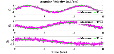
Figure 3: True and measured angular velocities.

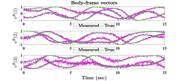
Figure 4: Body-frame vectorial measurements: true and measured.

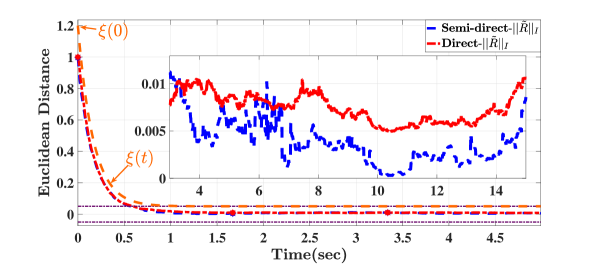
Figure 5: Transient and steady-state performance of normalized Euclidean distance.

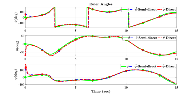
Figure 6: Tracking performance of Euler angles (roll $(\phi)$ and pitch $(\theta)$, yaw $(\psi)$).

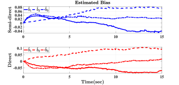
Figure 7: The estimated bias of the proposed filters.

Table I contains a synopsis of statistical details of the mean and the STD of the error ($||\tilde{R}||_{I}$). These details facilitate the comparison of the steady-state performance of the two filters proposed in this paper with respect to $||\tilde{R}||_{I}$. In spite of the fact that both filters have extremely small mean of $||\tilde{R}||_{I}$, the semi-direct attitude filter with prescribed performance showed a remarkably smaller mean errors and STD when compared to the direct attitude filter with prescribed performance. Numerical results outlined in Table I demonstrate effectiveness and robustness of the proposed nonlinear attitude filters against large error initialization and uncertainties in sensor measurements as illustrated in Figure 3, 4, 6, 5, and 7.

TABLE I: Statistical analysis of $||\tilde{R}||_{I}$ of the proposed two filters.

Output data of $||\tilde{R}||_{I}$ over the period (1-15 sec)
Filter	Semi-direct	Direct
Mean	$4.2\times 10^{-3}$	$6.9\times 10^{-3}$
STD	$2.5\times 10^{-3}$	$2.1\times 10^{-3}$

The robustness and the superior convergence properties of the proposed nonlinear attitude filters with guaranteed performance are presented and compared to a well-known nonlinear attitude complimentary filter termed nonlinear passive complementary filter [5] as well as to a standard attitude filter which belongs to the family of Gaussian attitude filters and is termed multiplicative extended Kalman filter (MEKF) [8] in Subsection V-A and V-B, respectively.

V-A Proposed Filters vs Nonlinear Attitude Filters

To further illustrate the robustness and the superior convergence properties of the proposed nonlinear attitude filters as opposed to the conventional nonlinear attitude filters, a fair comparison is presented. Consider the following nonlinear passive complementary filter given in [5]

$$\begin{cases}\dot{\hat{R}}&=\hat{R}\left[\Omega_{m}-\hat{b}-W\right]_{\times},\quad\hat{R}\left(0\right)=\hat{R}_{0}\\ \dot{\hat{b}}&=k_{1}\mathbf{vex}\left(\boldsymbol{\mathcal{P}}_{a}\left(\tilde{R}\right)\right),\quad\hat{b}\left(0\right)=\hat{b}_{0},\tilde{R}=R_{y}^{\top}\hat{R}\\ W&=k_{1}\mathbf{vex}\left(\boldsymbol{\mathcal{P}}_{a}\left(\tilde{R}\right)\right),\tilde{R}=R_{y}^{\top}\hat{R}\end{cases}$$ (61)

where $k_{1}>0$. A fair comparison between the proposed semi-direct attitude filter and the nonlinear passive complementary filter in [5] is attainable due to the shared structure of the filters. Consider initializing the nonlinear passive complementary filter analogously to the semi-direct attitude filter given at the beginning of the Simulation Section. To ensure validity of the comparison, three variations of the design parameter $k_{1}$ in (61) namely, $k_{1}=1$, $k_{1}=10$ and $k_{1}=100$.

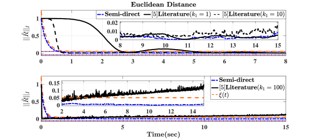
Figure 8: Transient and steady-state performance of normalized Euclidean distance: Semi-direct filter vs literature [5].

In this Subsection, the color notation is as follows: black solid and dashed lines describe the performance of the nonlinear passive complementary filter, blue center line depicts the proposed semi-direct attitude filter while orange and purple refer to the prescribed performance response. It can be noticed in the upper portion of Figure 8 that smaller value of $k_{1}$ results in slower transient performance with less oscillatory behavior in the steady-state. In contrast, the lower portion of Figure 8 illustrates that higher value of $k_{1}$ leads to faster transient performance with higher levels of oscillation in the steady-state. Moreover, Figure 8 shows that the predefined measure of transient performance cannot be achieved for low value of $k_{1}$, since the transient performance of the passive complementary filter violates the dynamic reducing boundaries. In the same spirit, the predefined characteristics of steady-state performance cannot be achieved for high value of $k_{1}$. These results confirm Remark 1.

Therefore, the nonlinear attitude filters given in the literature, for example [18, 5, 12, 14, 19, 13] cannot guarantee a predefined measure of convergence properties. The semi-direct attitude filter, on the other side, obeys the dynamically reducing boundaries and allows to achieve a desired level of prescribed performance.

Table II compares the statistical details, namely the mean and the STD of $||\tilde{R}||_{I}$, of the proposed semi-direct attitude filter and the nonlinear passive complementary filter. The above-mentioned statistics describe the output performance with respect to $||\tilde{R}||_{I}$ over the steady-state period of time depicted in Figure 8. The semi-direct attitude filter displays smaller values of mean and STD of $||\tilde{R}||_{I}$ when compared to the passive complementary filter for all the considered cases of $k_{1}=1$, $k_{1}=10$ and $k_{1}=100$. Moreover, the numerical results listed in Table II illustrate the effectiveness and robustness of the proposed nonlinear attitude filters against large error initialization and uncertainties in sensor measurements which make them a good fit for measurements obtained from low-cost IMUs modules.

TABLE II: Statistical analysis of $||\tilde{R}||_{I}$ of the semi-direct filter vs literature.

Output data of $||\tilde{R}||_{I}$ over the period (7-15 sec)
Filter	Semi-direct	Passive Filter [5]
		$k_{1}=1$	$k_{1}=10$	$k_{1}=100$
Mean	$2.7\times 10^{-3}$	$4.5\times 10^{-3}$	$6.9\times 10^{-3}$	$91.9\times 10^{-3}$
STD	$1.4\times 10^{-3}$	$2.9\times 10^{-3}$	$2.7\times 10^{-3}$	$14.2\times 10^{-3}$

V-B Proposed Filters vs Gaussian Attitude Filters

In this subsection the effectiveness and the high convergence capabilities of the proposed nonlinear attitude filters are compared to the performance of a Gaussian attitude filter. A comparison between the proposed direct attitude filter and the MEKF in Appendix C is presented. Consider the MEKF in Appendix C initialized similar to the direct attitude filter given at the beginning of the Simulation Section. To guarantee validity of the comparison, three cases of the design parameters of MEKF have been detailed in Table III.

TABLE III: MEKF design parameters.

Case	Design Parameters
Case 1	$\mathcal{\bar{Q}}_{v\left(i\right)}=\mathbf{I}_{3}$	$\mathcal{\bar{Q}}_{\omega}=\mathbf{I}_{3}$	$\mathcal{\bar{Q}}_{b}=\mathbf{I}_{3}$
Case 2	$\mathcal{\bar{Q}}_{v\left(i\right)}=0.1\mathbf{I}_{3}$	$\mathcal{\bar{Q}}_{\omega}=10\mathbf{I}_{3}$	$\mathcal{\bar{Q}}_{b}=10\mathbf{I}_{3}$
Case 3	$\mathcal{\bar{Q}}_{v\left(i\right)}=0.01\mathbf{I}_{3}$	$\mathcal{\bar{Q}}_{\omega}=100\mathbf{I}_{3}$	$\mathcal{\bar{Q}}_{b}=100\mathbf{I}_{3}$

In this Subsection, the color notation is as follows: black solid and dashed lines represent the performance of the MEKF, blue center line refers to the proposed direct attitude filter while orange and purple depict the prescribed performance response. It can be noticed in the upper portion of Figure 9 that cases 1 and 2 show slower transient performance with less oscillatory behavior in the steady-state. In contrast, the lower portion of Figure 9 illustrates that case 3 results in faster transient performance with higher levels of oscillation in the steady-state. As such, a desired measure of transient and stead-state error cannot be guaranteed in case of MEKF.

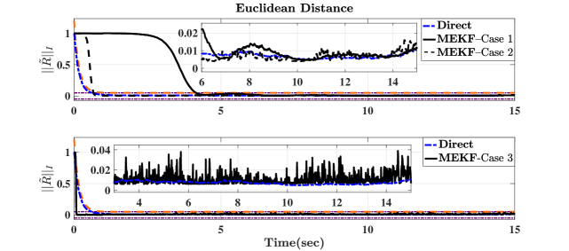
Figure 9: Transient and steady-state performance of normalized Euclidean distance: Direct filter vs MEKF [8].

The direct attitude filter, on the other side, follows the dynamically reducing boundaries achieving a desired level of prescribed performance set by the user.

The simulation results presented in this section validate the stable performance and robustness of the two proposed filters against uncertain measurements and large initialized errors. The two filters comply with the constraints imposed by the user indicating guaranteed prescribed performance measures in transient as well as steady-state performance. This remarkable advantage was not offered in other nonlinear deterministic attitude filters such as [18, 5, 12, 15, 14, 16, 19, 13] as well as Gaussian attitude filters such as [6, 7, 8]. Semi-direct attitude filter with prescribed performance requires attitude reconstruction, for instance in our case we employed SVD Appendix B, to obtain $\tilde{R}=R_{y}^{\top}\hat{R}$. This adds complexity, and therefore the semi-direct attitude filter requires more computational power in comparison with direct attitude filter with prescribed performance. However, both proposed filters showed remarkable convergence as detailed in Table I.

VI Conclusion

In this paper, two nonlinear attitude filters with prescribed performance characteristics have been considered. The filters are evolved directly on $\mathbb{SO}\left(3\right)$. Attitude error has been defined in terms of normalized Euclidean distance such that innovation term has been selected to ensure predefined characteristics of transient and steady-state performance. Consequently, the proposed filters achieve superior convergence properties with transient error being less than a predefined dynamic decreasing constrained function and steady-state error being confined by a known lower bound. The constrained error is transformed to its unconstrained form which is sufficient to solve the attitude problem in prescribed performance sense. The filters are deterministic while the stability analysis ensure boundedness of all closed loop signals with asymptotic convergence of the normalized Euclidean distance of attitude error to the origin. Simulation example illustrated the robustness of the proposed filters in their response to the predefined constraints in case when high level of uncertainties is present in the measurements and a large initial attitude error is observed.

Appendix A

Proof of Lemma 1

Let the attitude be represented by $R\in\mathbb{SO}\left(3\right)$. The attitude could be obtained knowing Rodriguez parameters vector $\rho\in\mathbb{R}^{3}$. It is worth mentioning that Rodriguez parameters vector $\rho$ is used for the sake of proving the results in Lemma 1. The related map from vector form to $\mathbb{SO}\left(3\right)$ is governed by $\mathcal{R}_{\rho}:\mathbb{R}^{3}\rightarrow\mathbb{SO}\left(3\right)$ [26] such that

$$\mathcal{R}_{\rho}\left(\rho\right)= \frac{1}{1+||\rho||^{2}}\left(\left(1-||\rho||^{2}\right)\mathbf{I}_{3}+2\rho\rho^{\top}+2\left[\rho\right]_{\times}\right)$$ (62)

with direct substitution of (62) in (1) one obtains

$$||R||_{I}=\frac{||\rho||^{2}}{1+||\rho||^{2}}$$ (63)

Likewise, the anti-symmetric projection operator of attitude $R$ in (62) for $\mathcal{R}_{\rho}=\mathcal{R}_{\rho}\left(\rho\right)$ can be defined as

$$\boldsymbol{\mathcal{P}}_{a}\left(R\right)=\frac{1}{2}\left(\mathcal{R}_{\rho}-\mathcal{R}_{\rho}^{\top}\right)= 2\frac{1}{1+||\rho||^{2}}\left[\rho\right]_{\times}$$

and the vex operator

$$\mathbf{vex}\left(\boldsymbol{\mathcal{P}}_{a}\left(R\right)\right)=2\frac{\rho}{1+||\rho||^{2}}$$ (64)

From (63) one can show that

$$\left(1-||R||_{I}\right)||R||_{I}=\frac{||\rho||^{2}}{\left(1+||\rho||^{2}\right)^{2}}$$ (65)

and from (64) one has

$$||\mathbf{vex}\left(\boldsymbol{\mathcal{P}}_{a}\left(R\right)\right)||^{2}=4\frac{||\rho||^{2}}{\left(1+||\rho||^{2}\right)^{2}}$$ (66)

Thus, (65) and (66) prove (16) in Lemma 1. From Subsection IV-B $\sum_{i=1}^{n}s_{i}=3$ which implies that ${\rm Tr}\left\{M^{\mathcal{B}}\right\}=3$ and the normalized Euclidean distance of $M^{\mathcal{B}}R$ is $||M^{\mathcal{B}}R||_{I}=\frac{1}{4}{\rm Tr}\left\{M^{\mathcal{B}}\left(\mathbf{I}_{3}-R\right)\right\}$. According to angle-axis parameterization in (2), one obtains

$$||M^{\mathcal{B}}R||_{I} =\frac{1}{4}{\rm Tr}\left\{-M^{\mathcal{B}}\left(\sin(\theta)\left[u\right]_{\times}+\left(1-\cos(\theta)\right)\left[u\right]_{\times}^{2}\right)\right\}$$

$$=-\frac{1}{4}{\rm Tr}\left\{M^{\mathcal{B}}\left(1-\cos(\theta)\right)\left[u\right]_{\times}^{2}\right\}$$ (67)

where ${\rm Tr}\left\{M^{\mathcal{B}}\left[u\right]_{\times}\right\}=0$ as given in identity (8). One has [25]

$$||R||_{I}=\frac{1}{4}{\rm Tr}\left\{\mathbf{I}_{3}-R\right\}=\frac{1}{2}\left(1-{\rm cos}\left(\theta\right)\right)={\rm sin}^{2}\left(\frac{\theta}{2}\right)$$ (68)

and the Rodriguez parameters vector in terms of angle-axis parameterization is [26]

$$u={\rm cot}\left(\frac{\theta}{2}\right)\rho$$

From identity (5) $\left[u\right]_{\times}^{2}=-||u||^{2}\mathbf{I}_{3}+uu^{\top}$, the expression in (67) becomes

$$||M^{\mathcal{B}}R||_{I} =\frac{1}{2}||R||_{I}u^{\top}\bar{\mathbf{M}}^{\mathcal{B}}u$$

$$=\frac{1}{2}||R||_{I}{\rm cot}^{2}\left(\frac{\theta}{2}\right)\rho^{\top}\bar{\mathbf{M}}^{\mathcal{B}}\rho$$

From (68), one can find ${\rm cos}^{2}\left(\frac{\theta}{2}\right)=1-||R||_{I}$ which means

$${\rm tan}^{2}\left(\frac{\theta}{2}\right)=\frac{||R||_{I}}{1-||R||_{I}}$$

Consequently, the normalized Euclidean distance is defined in the sense of Rodriguez parameters vector as

$$||M^{\mathcal{B}}R||_{I} =\frac{1}{2}\left(1-||R||_{I}\right)\rho^{\top}\bar{\mathbf{M}}^{\mathcal{B}}\rho$$

$$=\frac{1}{2}\frac{\rho^{\top}\bar{\mathbf{M}}^{\mathcal{B}}\rho}{1+||\rho||^{2}}$$ (69)

The anti-symmetric projection operator in terms of Rodriguez parameters vector with aid of identity (3) and (6) can be defined as

$$\boldsymbol{\mathcal{P}}_{a}\left(M^{\mathcal{B}}R\right)= \frac{M^{\mathcal{B}}\rho\rho^{\top}-\rho\rho^{\top}M^{\mathcal{B}}+M^{\mathcal{B}}\left[\rho\right]_{\times}+\left[\rho\right]_{\times}M^{\mathcal{B}}}{1+||\rho||^{2}}$$

$$= \frac{\left[\left({\rm Tr}\left\{M^{\mathcal{B}}\right\}\mathbf{I}_{3}-M^{\mathcal{B}}+\left[\rho\right]_{\times}M^{\mathcal{B}}\right)\rho\right]_{\times}}{1+||\rho||^{2}}$$

It follows that the vex operator of the above expression is

$$\mathcal{\mathbf{vex}}\left(\boldsymbol{\mathcal{P}}_{a}\left(M^{\mathcal{B}}R\right)\right) =\frac{1}{1+||\rho||^{2}}\left(\mathbf{I}_{3}-\left[\rho\right]_{\times}\right)\bar{\mathbf{M}}^{\mathcal{B}}\rho$$ (70)

The 2-norm of (70) can be obtained by

$$||\mathbf{vex}\left(\boldsymbol{\mathcal{P}}_{a}\left(M^{\mathcal{B}}R\right)\right)||^{2} =\frac{\rho^{\top}\bar{\mathbf{M}}^{\mathcal{B}}\left(\mathbf{I}_{3}-\left[\rho\right]_{\times}^{2}\right)\bar{\mathbf{M}}^{\mathcal{B}}\rho}{\left(1+||\rho||^{2}\right)^{2}}$$

with the aid of identity (5) $\left[\rho\right]_{\times}^{2}=-||\rho||^{2}\mathbf{I}_{3}+\rho\rho^{\top}$, one obtains

$$||\mathbf{vex}\left(\boldsymbol{\mathcal{P}}_{a}\left(M^{\mathcal{B}}R\right)\right)||^{2} =\frac{\rho^{\top}\bar{\mathbf{M}}^{\mathcal{B}}\left(\mathbf{I}_{3}-\left[\rho\right]_{\times}^{2}\right)\bar{\mathbf{M}}^{\mathcal{B}}\rho}{\left(1+||\rho||^{2}\right)^{2}}$$

$$=\frac{\rho^{\top}\left(\bar{\mathbf{M}}^{\mathcal{B}}\right)^{2}\rho}{1+||\rho||^{2}}-\frac{\left(\rho^{\top}\bar{\mathbf{M}}^{\mathcal{B}}\rho\right)^{2}}{\left(1+||\rho||^{2}\right)^{2}}$$

$$\geq\underline{\lambda}\left(1-\frac{\left\|\rho\right\|^{2}}{1+\left\|\rho\right\|^{2}}\right)\frac{\rho^{\top}\bar{\mathbf{M}}^{\mathcal{B}}\rho}{1+||\rho||^{2}}$$ (71)

where $\underline{\lambda}=\underline{\lambda}\left(\bar{\mathbf{M}}^{\mathcal{B}}\right)$ is the minimum singular value of $\bar{\mathbf{M}}^{\mathcal{B}}$ and $\left\|R\right\|_{I}=\frac{\left\|\rho\right\|^{2}}{1+\left\|\rho\right\|^{2}}$ as defined in (63). It can be found that

$$1-\left\|R\right\|_{I} ={\rm Tr}\left\{\frac{1}{12}\mathbf{I}_{3}+\frac{1}{4}R\right\}$$

$$={\rm Tr}\left\{\frac{1}{12}\mathbf{I}_{3}+\frac{1}{4}\left(M^{\mathcal{B}}\right)^{-1}M^{\mathcal{B}}R\right\}$$ (72)

Therefore, from (71), and (72) the following inequality holds

$$||\mathbf{vex}\left(\boldsymbol{\mathcal{P}}_{a}\left(M^{\mathcal{B}}R\right)\right)||^{2}$$

$$\hskip 50.00008pt\geq\frac{\underline{\lambda}}{2}\left(1+{\rm Tr}\left\{\left(M^{\mathcal{B}}\right)^{-1}M^{\mathcal{B}}R\right\}\right)\left\|M^{\mathcal{B}}R\right\|_{I}$$

which proves (17) in Lemma 1.

Appendix B

An Overview on SVD in [3]

Let the true attitude be $R\in\mathbb{SO}\left(3\right)$. A set of vectors presented in (11) could be utilized to reconstruct the attitude. Define $s_{i}$ as the confidence level the $i$th measurement and for $n$ measurements. Define $s_{i}=\frac{s_{i}}{\sum_{i=1}^{n}s_{i}}$. Accordingly, the corrupted reconstructed attitude $R_{y}$ is given by

$$\begin{cases}\mathcal{J}\left(R\right)&=1-\sum_{i=1}^{n}s_{i}\left(\upsilon_{i}^{\mathcal{B}}\right)^{\top}R^{\top}\upsilon_{i}^{\mathcal{I}}\\ &=1-{\rm Tr}\left\{R^{\top}B^{\top}\right\}\\ B&=\sum_{i=1}^{n}s_{i}\upsilon_{i}^{\mathcal{B}}\left(\upsilon_{i}^{\mathcal{I}}\right)^{\top}=USV^{\top}\\ U_{+}&=U\left[\begin{array}[]{ccc}1&0&0\\ 0&1&0\\ 0&0&{\rm det}\left(U\right)\end{array}\right]\\ V_{+}&=V\left[\begin{array}[]{ccc}1&0&0\\ 0&1&0\\ 0&0&{\rm det}\left(V\right)\end{array}\right]\\ R_{y}&=V_{+}U_{+}^{\top}\end{cases}$$

For more details consult [3] or see the Appendix in [15].

Appendix C

An Overview of MEKF in [8, 29]

The unit-quaternion vector $Q=\left[q_{0},q^{\top}\right]^{\top}\in\mathbb{S}^{3}$ is composed of a scalar component $q_{0}\in\mathbb{R}$ and a vector $q\in\mathbb{R}^{3}$ defined by

$$\mathbb{S}^{3}=\left\{\left.Q\in\mathbb{R}^{4}\right|\left\|Q\right\|=1\right\}$$

The structure of MEKF is as follows

$$\Psi\left(x\right) =\left[\begin{array}[]{cc}0&-x^{\top}\\ x&-\left[x\right]_{\times}\end{array}\right]\in\mathbb{R}^{4\times 4},\hskip 10.00002ptx\in\mathbb{R}^{3\times 1}$$ (75)

$$\dot{\hat{Q}} =\frac{1}{2}\Psi\left(\Omega_{m}-\hat{b}+P_{a}W\right)\hat{Q}$$

$$W =\sum_{i=1}^{n}\hat{\upsilon}_{i}^{\mathcal{B}}\times\mathcal{\bar{Q}}_{v\left(i\right)}^{-1}\left(\hat{\upsilon}_{i}^{\mathcal{B}}-\upsilon_{i}^{\mathcal{B}}\right)$$

$$\left[\begin{array}[]{c}0\\ W\end{array}\right] =\sum_{i=1}^{n}\left[\begin{array}[]{c}0\\ \hat{\upsilon}_{i}^{\mathcal{B}}\end{array}\right]\times\left[\begin{array}[]{cc}0&0_{3\times 1}^{\top}\\ 0_{3\times 1}&\mathcal{\bar{Q}}_{v\left(i\right)}^{-1}\end{array}\right]\left[\begin{array}[]{c}0\\ \hat{\upsilon}_{i}^{\mathcal{B}}-\upsilon_{i}^{\mathcal{B}}\end{array}\right]$$ (84)

$$\left[\begin{array}[]{c}0\\ \hat{\upsilon}_{i}^{\mathcal{B}}\end{array}\right] =\hat{Q}^{-1}\odot\left[\begin{array}[]{c}0\\ \upsilon_{i}^{\mathcal{I}}\end{array}\right]\odot\hat{Q}$$ (89)

where $\hat{Q}\in\mathbb{S}^{3}$ denotes the estimate of the true unit-quaternion, $\odot$ denotes unit-quaternion multiplication, $\upsilon_{i}^{\mathcal{B}},\upsilon_{i}^{\mathcal{I}}\in\mathbb{R}^{3}$ are defined in (10) and (11), and

$$\begin{cases}\boldsymbol{\mathcal{P}}_{s}\left(A\right)&=\frac{1}{2}\left(A+A^{\top}\right),\hskip 10.00002ptA\in\mathbb{R}^{3\times 3}\\ \dot{\hat{b}}&=P_{c}^{\top}W\\ S&=\sum_{i=1}^{n}\left[\hat{\upsilon}_{i}^{\mathcal{B}}\right]_{\times}\mathcal{\bar{Q}}_{v\left(i\right)}^{-1}\left[\hat{\upsilon}_{i}^{\mathcal{B}}\right]_{\times}\\ \dot{P}_{a}&=\mathcal{\bar{Q}}_{\omega}+2\boldsymbol{\mathcal{P}}_{s}\left(P_{a}\left[\Omega_{m}-\hat{b}\right]_{\times}-P_{c}\right)\\ &\hskip 10.00002pt-P_{a}SP_{a}\\ \dot{P}_{b}&=\mathcal{\bar{Q}}_{b}-P_{c}SP_{c}\\ \dot{P}_{c}&=-\left[\Omega_{m}-\hat{b}\right]_{\times}P_{c}-P_{a}SP_{c}-P_{b}\end{cases}$$ (90)

with $\mathcal{\bar{Q}}_{v\left(i\right)},\mathcal{\bar{Q}}_{\omega},\mathcal{\bar{Q}}_{b}\in\mathbb{R}^{3\times 3}$ being covariance matrices, for $i=1,2,\ldots,n$. The rest of the notation is identical to the notation used in the filter design given before Theorem 1 and 2.

AUTHOR INFORMATION

Hashim A. Hashim is a Ph.D. candidate and a Teaching and Research Assistant in Robotics and Control, Department of Electrical and Computer Engineering at the University of Western Ontario, ON, Canada.
His current research interests include stochastic and deterministic filters on SO(3) and SE(3), control of multi-agent systems, control applications and optimization techniques.
Contact Information: hmoham33@uwo.ca.

Lyndon J. Brown received the B.Sc. degree from the U. of Waterloo, Canada in 1988 and the M.Sc. and PhD. degrees from the University of Illinois, Urbana-Champaign in 1991 and 1996, respectively. He is an associate professor in the department of electrical and computer engineering at Western University, Canada. He worked in industry for Honeywell Aerospace Canada and E.I. DuPont de Nemours.
His current research includes the identification and control of predictable signals, biological control systems, welding control systems, attitude and pose estimation.

Kenneth McIsaac received the B.Sc. degree from the University of Waterloo, Canada, in 1996, and the M.Sc. and Ph.D. degrees from the University of Pennsylvania, in 1998 and 2001, respectively. He is currently an Associate Professor and the Chair of Electrical and Computer Engineering with Western University, ON, Canada.
His current research interests include computer vision and signal processing, mostly in the context of using machine intelligence in robotics and assistive systems. Also, his research interests include attitude and pose estimation.

References

• [1] H. D. Black, “A passive system for determining the attitude of a satellite,” AIAA journal, vol. 2, no. 7, pp. 1350–1351, 1964.
• [2] M. D. Shuster and S. D. Oh, “Three-axis attitude determination from vector observations,” Journal of Guidance, Control, and Dynamics, vol. 4, pp. 70–77, 1981.
• [3] F. L. Markley, “Attitude determination using vector observations and the singular value decomposition,” Journal of the Astronautical Sciences, vol. 36, no. 3, pp. 245–258, 1988.
• [4] J. L. Crassidis, F. L. Markley, and Y. Cheng, “Survey of nonlinear attitude estimation methods,” Journal of guidance, control, and dynamics, vol. 30, no. 1, pp. 12–28, 2007.
• [5] R. Mahony, T. Hamel, and J.-M. Pflimlin, “Nonlinear complementary filters on the special orthogonal group,” IEEE Transactions on Automatic Control, vol. 53, no. 5, pp. 1203–1218, 2008.
• [6] E. J. Lefferts, F. L. Markley, and M. D. Shuster, “Kalman filtering for spacecraft attitude estimation,” Journal of Guidance, Control, and Dynamics, vol. 5, no. 5, pp. 417–429, 1982.
• [7] D. Choukroun, I. Y. Bar-Itzhack, and Y. Oshman, “Novel quaternion kalman filter,” IEEE Transactions on Aerospace and Electronic Systems, vol. 42, no. 1, pp. 174–190, 2006.
• [8] F. L. Markley, “Attitude error representations for kalman filtering,” Journal of guidance, control, and dynamics, vol. 26, no. 2, pp. 311–317, 2003.
• [9] B. N. Stovner, T. A. Johansen, T. I. Fossen, and I. Schjølberg, “Attitude estimation by multiplicative exogenous kalman filter,” Automatica, vol. 95, pp. 347–355, 2018.
• [10] S. Bonnable, P. Martin, and E. Salaün, “Invariant extended kalman filter: theory and application to a velocity-aided attitude estimation problem,” in Decision and Control, 2009 held jointly with the 2009 28th Chinese Control Conference. CDC/CCC 2009. Proceedings of the 48th IEEE Conference on.   IEEE, 2009, pp. 1297–1304.
• [11] M. Zamani, J. Trumpf, and R. Mahony, “Minimum-energy filtering for attitude estimation,” IEEE Transactions on Automatic Control, vol. 58, no. 11, pp. 2917–2921, 2013.
• [12] T. Hamel and R. Mahony, “Attitude estimation on so [3] based on direct inertial measurements,” in Robotics and Automation, 2006. ICRA 2006. Proceedings 2006 IEEE International Conference on.   IEEE, 2006, pp. 2170–2175.
• [13] D. E. Zlotnik and J. R. Forbes, “Nonlinear estimator design on the special orthogonal group using vector measurements directly,” IEEE Transactions on Automatic Control, vol. 62, no. 1, pp. 149–160, 2017.
• [14] H. F. Grip, T. I. Fossen, T. A. Johansen, and A. Saberi, “Attitude estimation using biased gyro and vector measurements with time-varying reference vectors,” IEEE Transactions on Automatic Control, vol. 57, no. 5, pp. 1332–1338, 2012.
• [15] H. A. Hashim, L. J. Brown, and K. McIsaac, “Nonlinear stochastic attitude filters on the special orthogonal group 3: Ito and stratonovich,” IEEE Transactions on Systems, Man, and Cybernetics: Systems, pp. 1–13, 2018.
• [16] H. A. Hashim, L. J. Brown, and K. McIsaac, “Nonlinear explicit stochastic attitude filter on so(3),” in Proceedings of the 57th IEEE conference on Decision and Control (CDC).   IEEE, 2018, pp. 1–7.
• [17] J. Wu, Z. Zhou, B. Gao, R. Li, Y. Cheng, and H. Fourati, “Fast linear quaternion attitude estimator using vector observations,” IEEE Transactions on Automation Science and Engineering, vol. 15, no. 1, pp. 307–319, 2018.
• [18] R. Mahony, T. Hamel, and J.-M. Pflimlin, “Complementary filter design on the special orthogonal group so (3),” in Decision and Control, 2005 and 2005 European Control Conference. CDC-ECC’05. 44th IEEE Conference on.   IEEE, 2005, pp. 1477–1484.
• [19] T. Lee, “Exponential stability of an attitude tracking control system on so (3) for large-angle rotational maneuvers,” Systems & Control Letters, vol. 61, no. 1, pp. 231–237, 2012.
• [20] C. P. Bechlioulis and G. A. Rovithakis, “Robust adaptive control of feedback linearizable mimo nonlinear systems with prescribed performance,” IEEE Transactions on Automatic Control, vol. 53, no. 9, pp. 2090–2099, 2008.
• [21] H. A. H. Mohamed, “Improved robust adaptive control of high-order nonlinear systems with guaranteed performance,” M. Sc, King Fahd University Of Petroleum & Minerals, vol. 1, 2014.
• [22] L. Zhu, Y. Zhou, and Y. Liu, “Robust adaptive neural prescribed performance control for mdf continuous hot pressing system with input saturation,” IEEE ACCESS, vol. 6, pp. 9099–9113, 2018.
• [23] H. A. Hashim, S. El-Ferik, and F. L. Lewis, “Neuro-adaptive cooperative tracking control with prescribed performance of unknown higher-order nonlinear multi-agent systems,” International Journal of Control, pp. 1–16, 2017.
• [24] H. A. Hashim, S. El-Ferik, and F. L. Lewis, “Adaptive synchronisation of unknown nonlinear networked systems with prescribed performance,” International Journal of Systems Science, vol. 48, no. 4, pp. 885–898, 2017.
• [25] R. M. Murray, Z. Li, S. S. Sastry, and S. S. Sastry, A mathematical introduction to robotic manipulation.   CRC press, 1994.
• [26] M. D. Shuster, “A survey of attitude representations,” Navigation, vol. 8, no. 9, pp. 439–517, 1993.
• [27] H. A. Hashim, L. J. Brown, and K. McIsaac, “Nonlinear stochastic position and attitude filter on the special euclidean group 3,” Journal of the Franklin Institute, pp. 1–27, 2018.
• [28] F. Bullo and A. D. Lewis, Geometric control of mechanical systems: modeling, analysis, and design for simple mechanical control systems.   Springer Science & Business Media, 2004, vol. 49.
• [29] M. Zamani, J. Trumpf, and R. Mahony, “Nonlinear attitude filtering: A comparison study,” arXiv preprint arXiv:1502.03990, 2015.