Regime transitions and energetics of sustained stratified shear flows

Abstract

We describe the long-term dynamics of sustained stratified shear flows in the laboratory. The Stratified Inclined Duct (SID) experiment sets up a two-layer exchange flow in an inclined duct connecting two reservoirs containing salt solutions of different densities. This flow is primarily characterised by two non-dimensional parameters: the tilt angle of the duct with respect to the horizontal, $\theta$ (a few degrees at most), and the Reynolds number $Re$, an input parameter based on the density difference driving the flow. The flow can be sustained with constant forcing over arbitrarily long times and exhibits a wealth of dynamical behaviours representative of geophysically-relevant sustained stratified shear flows. Varying $\theta$ and $Re$ leads to four qualitatively different regimes: laminar flow; mostly laminar flow with finite-amplitude, travelling Holmboe waves; spatio-temporally intermittent turbulence with substantial interfacial mixing; and sustained, vigorous interfacial turbulence (Meyer & Linden, J. Fluid Mech., vol. 753, 2014, pp. 242–253). We seek to explain the scaling of the transitions between flow regimes in the two-dimensional plane of input parameters $(\theta,Re)$. We improve upon previous studies of this problem by providing a firm physical basis and non-dimensional scaling laws that are mutually consistent and in good agreement with the empirical transition curves we inferred from 360 experiments spanning $\theta\in[-1^{\circ},6^{\circ}]$ and $Re\in[300,5000]$. To do so, we employ state-of-the-art simultaneous volumetric measurements of the density field and the three-component velocity field, and analyse these experimental data using time- and volume-averaged potential and kinetic energy budgets. We show that regime transitions are caused by an increase in the non-dimensional time- and volume-averaged kinetic energy dissipation within the duct, which scales with $\theta Re$ at high enough angles. As the power input scaling with $\theta Re$ is increased above zero, the two-dimensional, parallel-flow dissipation (power output) increases to close the budget through an increase in the magnitude of the exchange flow, incidentally triggering Holmboe waves above a certain threshold in interfacial shear. However, once the hydraulic limit of two-layer exchange flows is reached, two-dimensional dissipation plateaus and three-dimensional dissipation at small scales (turbulence) takes over, first intermittently, and then steadily, in order to close the budget and follow the $\theta Re$ scaling. This general understanding of regime transitions and energetics in the SID experiment may serve as a basis for the study of more complex sustained stratified shear flows found in the natural environment.

1 Introduction

Turbulence is still an ‘unsolved problem’, and the stabilising buoyancy forces that characterise stratified turbulence add further complexity. The spatio-temporal scales involved in the physics of (stratified) turbulent flows make them very difficult to understand with our current computational capabilities and brain power.

The historical and dominant angle of attack to this problem is to attempt to model the ‘small-scale’ (inaccessible) physics of turbulence and mixing using the ‘large-scale’ (accessible) properties of the flows. A much-pursued goal is the ability, for any given flow, to predict its regime (e.g. laminar, intermittently turbulent, fully turbulent), rate of energy dissipation and mixing efficiency (so-called ‘outputs’ variables) using only a small number of ‘input’ non-dimensional parameters characterising the flow (for four decades of reviews on mixing efficiency, see e.g. linden_mixing_1979; fernando_turbulent_1991; ivey_density_2008; gregg_mixing_2018). Drawing on the power of dimensional analysis and theoretical scaling laws, the hope is that empirical relationships obtained under controlled conditions can then be extrapolated beyond laboratory or simulated scales. Following this tradition of research, the aim of this paper is the quantitative study of flow regimes, and particularly of the transitions between them, from a non-dimensional perspective.

Stably stratified shear flows are a class of flows particularly relevant to the environment. Many of these flows are sustained over long periods of time through quasi-steady forcing: for example exchange flows in straits, estuaries (e.g. geyer_mixing_2010), coastal inlets (e.g. farmer_stratified_1999), deep ocean overflows (e.g. van_haren_extremely_2014) and stratified flows in the atmospheric boundary layer (e.g. mahrt_stably_2014). In this paper, we address these general and geophysically-relevant sustained stratified shear flows using a simple laboratory experiment: the Stratified Inclined Duct experiment.

2 The Stratified Inclined Duct (SID) experiment

We introduce the experiment central to this paper in § 2.1, and our experimental measurements and flow regime visualisations in § 2.2. We discuss the distribution of flow regimes in the space of input parameters and motivate this paper by reviewing the most relevant literature in § 2.3. We then build on the previous sections to reformulate the above aim in more specific terms and outline the paper in § 2.4.

2.1 Setup, notation and non-dimensionalisation

The Stratified Inclined Duct experiment (hereafter abbreviated SID) is sketched in figure 1. This conceptually simple experiment consists of two reservoirs initially filled with aqueous salt solutions of different densities $\rho_{0}\pm\Delta\rho/2$, connected by a long rectangular duct that can be tilted at a small angle $\theta$ from the horizontal (this is made possible by a flexible seal between the duct and the barrier separating the two reservoirs). At the start of the experiment, the duct is opened. After a brief transient gravity current, a two-layer exchange flow is sustained for long periods of time in the duct. This sustained stratified shear flow is the focus of this paper.

This flow is driven by two distinct forcing mechanisms: (i) a horizontal hydrostatic pressure gradient of opposite sign in each layer, resulting from each end of the duct sitting in reservoirs containing fluids of different densities, which is present even when the duct is horizontal (i.e when $\theta=0^{\circ}$); (ii) the gravitational acceleration of the buoyant layer upward (to the left) and the dense layer downward (to the right) when the tilt angle is positive $\theta>0^{\circ}$, defined here by the duct being raised in the denser reservoir, as shown in figure 1. The relative influence of these two forcing mechanisms will be discussed in § LABEL:sec:two-layer-model.

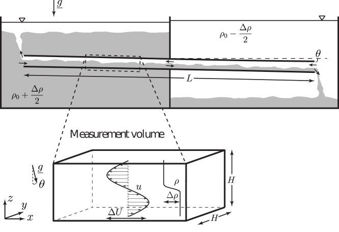
Figure 1: Schematics of the Stratified Inclined Duct (SID) experiment. The measurement volume inset shows the coordinate system and the notation used in this paper (in dimensional units). Note that the $x$ axis is aligned along the duct, resulting in gravity pointing at an angle $\theta$ from the $-z$ direction. Here, by definition, the duct is inclined at a positive angle $\theta>0^{\circ}$, resulting in a positive forcing of the flow by the streamwise projection of gravity $g\sin\theta>0$.

To the authors’ knowledge, the SID experiment was first studied by macagno_interfacial_1961. It was independently ‘rediscovered’ by kiel_buoyancy_1991 and more recently by meyer_stratified_2014 (hereafter ML14), who coined the name. ML14 correctly recognised that the two-layer exchange flow was maximal because it is hydraulically controlled at both ends of the duct where it meets the reservoirs through a sharp change in geometry (an idea already present in wilkinson_buoyancy_1986). In other words, the flow is subcritical with respect to long interfacial waves inside the duct, and critical at either end, preventing the propagation of information (in particular of the exchange flow rate) from the exterior into the duct (see ML14, lefauve_structure_2018, § 3, and lefauve_waves_2018, § 1.3.2 for more details). The exchange flow is sustained in a quasi-steady state until the controls are ‘flooded’ by the accumulation of fluid of a different density coming from the other reservoir. With each reservoirs holding approximately 100 l of fluid in our current setup, a typical experiment can last several minutes, which represents many duct transit times.

Our notation is shown in the measurement volume inset in figure 1 and follows that of lefauve_structure_2018 (hereafter LPZCDL18). The duct considered in this paper has length $L=1350$ mm and a square cross-section of $H=45$ mm (the same dimensions as LPZCDL18 but smaller than ML14). The streamwise $x$ axis is aligned along the duct and the spanwise $y$ axis across the duct, making the $z$ axis tilted at an angle $\theta$ from the vertical (resulting in a non-zero streamwise projection of gravity $g\sin\theta$ providing the gravitational forcing). All coordinates are centred in the middle of the duct, such that $-L/2\leq x\leq L/2$ and $-H/2\leq y,z\leq H/2$. The velocity vector field has components $\textbf{u}(x,y,z,t)=(u,v,w)$ along $x,y,z$, and we denote the density field by $\rho(x,y,z,t)$.

The parameters believed to play important roles are the geometrical parameters: $L$, $H$, $\theta$, and the dynamical parameters: the reduced gravity $g^{\prime}\equiv g\Delta\rho/\rho_{0}$ (under the Boussinesq approximation of small density differences $0<\Delta\rho/\rho_{0}\ll 1$), the kinematic viscosity of water $\nu=1.05\times 10^{-6}$ m${}^{2}$ s${}^{-1}$ and the molecular diffusivity of salt $\kappa_{s}=1.50\times 10^{-9}$ m${}^{2}$ s${}^{-1}$. From these six parameters having two dimensions (of length and time), we construct four independent non-dimensional parameters below.

In this maximal exchange flow, the velocity scale $\Delta U$ is not an independent parameter; it is primarily set by the phase speed of long interfacial gravity waves. To understand this, we follow the literature (see e.g. armi_hydraulics_1986; lawrence_hydraulics_1990) and define the composite Froude number of this two-layer flow as

$$G^{2}(x)\equiv F_{1}^{2}(x)+F_{2}^{2}(x),\quad\textrm{where}\quad F_{i}^{2}(x)\equiv\frac{\langle u_{i}^{2}(x)\rangle_{y,z_{i}}}{g^{\prime}h_{i}(x)}$$ (1)

is the Froude number of layer $i$, $\langle\cdot\rangle_{y,z_{i}}$ denotes spanwise and vertical averaging over the depth $h_{i}$ of each layer, and the symbol $\equiv$ denotes a definition. In the idealised case of frictionless, horizontal ducts ($\theta=0^{\circ}$), the flow is streamwise invariant and $G$ takes everywhere the value at the centre of the duct

$$G(x)=G(0)=2\frac{\langle|u|\rangle_{y,z}}{\sqrt{g^{\prime}H}},$$ (2)

where $\langle\cdot\rangle_{y,z}$ denotes averaging over the whole duct cross section. The second equality results from (1) and the symmetry of the flow at $x=0$ guaranteed by the Boussinesq approximation ($\langle|u_{1}|\rangle_{y,z}=\langle|u_{2}|\rangle_{y,z}$ and $h_{1}=h_{2}=H/2$). Note that here and in the remainder of the paper, we assume that the exchange flow has zero net (or ‘barotropic’) flow rate, i.e.

$$\langle u\rangle_{y,z}=0,$$ (3)

which is a good approximation in the present setup. Hydraulic control requires that $G^{2}\equiv 1$ (armi_hydraulics_1986), which gives the following layer-averaged velocity

$$\langle|u|\rangle_{y,z}=\frac{\sqrt{g^{\prime}H}}{2}.$$ (4)

With the addition of viscous friction and/or of a non-zero tilt angle, the flow is no longer streamwise invariant: $G(x)$ is maximal at the ends ($x=\pm L/2$) and minimal in the centre ($x=0$). Since the criticality condition is imposed at the ends where the controls occur $G(\pm L/2)=1>G(0)$, the velocity scale $\langle|u|\rangle_{y,z}=(\sqrt{g^{\prime}H}/2)G(0)$ is lower than the inviscid upper bound (4) that we call ‘hydraulic limit’ (see gu_analytical_2005 for more details). As first observed in ML14 (see their figure 7) and as we shall substantiate in § LABEL:sec:two-layer-model, this hydraulic limit is however generally achieved when a positive tilt angle $\theta>0^{\circ}$ is added to counterbalance the dissipative effects of viscosity.

Due to the moderate Reynolds numbers and the long duct investigated in the present setup, the velocity profiles are usually significantly affected by viscosity in the sense that viscous boundary layers at the walls and interface are partially or fully developed. Generally, we find that the peak velocities in each layer are at most around twice the layer-averaged values corresponding to the hydraulic limit (4), i.e. $\max_{y,z}|u|\approx 2\langle|u|\rangle_{y,z}\approx\sqrt{g^{\prime}H}$. We choose to non-dimensionalise velocities by this characteristic ‘peak’ value, i.e. half the total (peak-to-peak) velocity jump $\Delta U$ (shown in the inset in figure 1)

$$\frac{\Delta U}{2}\equiv\sqrt{g^{\prime}H}.$$ (5)

We thus define the non-dimensional velocity vector as $\tilde{\textbf{u}}\equiv\textbf{u}/(\Delta U/2)$ such that in general $-1\lesssim\tilde{u}\lesssim 1$ (noting that the streamwise velocity is dominant in this flow, i.e. $|\tilde{u}|\gg|\tilde{v}|,|\tilde{w}|$). For consistency, we choose $H/2$ as the length scale, defining the non-dimensional position vector as $\tilde{\textbf{x}}\equiv\textbf{x}/(H/2)$ such that $-1\leq\tilde{y},\tilde{z}\leq 1$, and $-A\leq\tilde{x}\leq A$, where the aspect ratio of the duct is

$$A\equiv\frac{L}{H}.$$ (6)

Consequently, we non-dimensionalise time by the advective time unit $H/\Delta U=1/(2\sqrt{g^{\prime}/H})$: $\tilde{t}\equiv 2\sqrt{g^{\prime}/H}t$ (hereafter abbreviated ATU). The dimensionless density field is defined as $\tilde{\rho}\equiv(\rho-\rho_{0})/(\Delta\rho/2)$, such that $-1\leq\tilde{\rho}\leq 1$.

Using the previously defined velocity and length scales, we construct the Reynolds number

$$Re\equiv\frac{\frac{\Delta U}{2}\frac{H}{2}}{\nu}=\frac{\sqrt{g^{\prime}H}H}{2\nu}=1.42\times 10^{4}\,\sqrt{\frac{\Delta\rho}{\rho_{0}}},$$ (7)

where the last equality shows that $Re$ is a function of the driving density difference $\Delta\rho/\rho_{0}$ alone (the prefactor only holds for aqueous salt solutions in the geometry investigated here). In this paper, we present experiments in the range $\Delta\rho/\rho_{0}\in[5\times 10^{-4},1.3\times 10^{-1}]$, i.e. $Re\in[300,5000]$.

The criticality condition $G^{2}=1$ adds another dimensional parameter, $\Delta U$, to our previous set of six input parameters. This velocity scale set by the criticality of the exchange flow can be recast as an overall Richardson number, expressed as the non-dimensional product of the density, length and inverse square velocity scales, and which here takes a constant value

$$Ri\equiv\frac{\frac{g}{\rho_{0}}\frac{\Delta\rho}{2}\frac{H}{2}}{\Big{(}\frac{\Delta U}{2}\Big{)}^{2}}=\frac{1}{4},$$ (8)

by definition of $\Delta U$ in (5).

Our last non-dimensional parameter is the Schmidt number, the ratio of the momentum to salt diffusivity

$$Sc\equiv\frac{\nu}{\kappa_{s}}.$$ (9)

In summary, we have a total of four free independent non-dimensional input parameters: $\theta$, $A$, $Re$, $Sc$, and one imposed parameter $Ri$. For the apparatus considered, we have $A=30$, $Sc=700$, $Ri=1/4$, and we have the freedom to vary $\theta$ and $Re$ (by varying $\Delta\rho/\rho_{0}$), allowing us access to a wide range of flow regimes as ML14 demonstrated and as we show in § 2.2-2.3. Henceforth, we drop the tildes and, unless explicitly stated otherwise, use non-dimensional variables throughout.

2.2 Measurements

In this section we introduce the three types of experimental measurements discussed in this paper: shadowgraph; mass flux; and volumetric three-dimensional, three-component (3D-3C) measurements of the velocity and density fields. We then discuss 3D-3C visualisations of flows in each regime to highlight some key features.

2.2.1 Shadowgraph

Shadowgraph observations of the flow in the duct were employed by ML14 to identify and classify four qualitatively different flow regimes depending on $\theta$ and $Re$ (see their figure 3) that they called L, H, I and T:

• L : Laminar steady flow, with a thin, flat density interface between the two counter-flowing layers;

• H : mostly laminar flow, with finite-amplitude Holmboe waves propagating on the interface;

• I : spatio-temporally Intermittent turbulence with small-scale structures and mixing that are conspicuous in the shadowgraph;

• T : steadily sustained Turbulence with significant small-scale structures and a thick interfacial mixing layer.

In this paper, we followed ML14 and carried out similar shadowgraph observations in our setup to classify hundreds of observed flows into these four qualitative regimes: (note that they are identical to those described in macagno_interfacial_1961, despite ML14 not being aware of their work).

2.2.2 Mass flux

We first define the instantaneous ‘volume flux’ $Q>0$, or exchange volume flow rate defined as the duct-averaged absolute value of the streamwise velocity:

$$Q(t)\equiv\langle|u|\rangle_{x,y,z},$$ (10)

where we recall that we assume no net flow, i.e. $\langle u\rangle_{x,y,z}=0$.

By analogy, we define the instantaneous ‘mass flux’ $Q_{m}>0$, or exchange mass flow rate as

$$Q_{m}(t)\equiv\langle\rho u\rangle_{x,y,z}$$ (11)

The $x$-averaging in these definitions is, strictly-speaking, unnecessary by conservation of volume along the duct, but we retain it as it will be employed to reduce experimental noise when evaluating $Q$ and $Q_{m}$ using three-dimensional data of $u(x,y,z)$ later. Note that $Q_{m}=Q$ in the absence of net flow and mixing (since in this case $\rho=\mathrm{sgn}(u)$), but in general $0<Q_{m}<Q$ in the presence of mixing (the distribution of $\rho$ is no longer bimodal and becomes continuous).

In a subset of the experiments in which shadowgraph observations were made, we also carried out mass flux measurements of $\langle Q_{m}\rangle_{t}$, where $\langle\cdot\rangle_{t}$ denotes averaging over the length of an experimental run. They were carried out as in ML14 using salt mass balances, i.e. by measuring the mean density of the solutions in each reservoir ($\rho_{0}\pm\Delta\rho/2$) before and after the experiment (for more details see lefauve_waves_2018, § 2.2, hereafter L18). Note the relation between our time-averaged mass flux and its equivalent definition in ML14, who called it the ‘Froude number’ $F\equiv\sqrt{2}\langle Q_{m}\rangle_{t}$.

The hydraulic limit for the volume flux set by the maximal exchange flow condition (4) can be rewritten in non-dimensional form as $Q=0.5$ (non-dimensionalising $u$ by (5)). We therefore have in general

$$0<Q_{m}\leq Q\leq 0.5.$$ (12)

The first two inequalities always hold by definition whereas the last inequality is the theoretical hydraulic limit that does not always hold in the experiments (we occasionally measured up to $Q_{m}\approx 0.6$).

2.2.3 Volumetric three-dimensional, three-component (3D-3C) measurements

To provide a quantitative basis to the qualitative shadowgraph observations and subsequent categorisation into flow regimes, we investigate in this paper the detailed energetics underpinning each regime. To do so, we employed simultaneous measurements of the density field and three-dimensional, three-component (3D-3C) velocity field in a volume, as sketched in the inset of figure 1.

These measuremements relied on a novel technique introduced by partridge_new_2018 in which a thin, pulsed vertical laser sheet (in the $x-z$ plane) is scanned rapidly back and forth in the spanwise direction (along $y$) to span a duct subvolume of non-dimensional cross-section $2\times 2$ and non-dimensional length $\ell$ (typically a small fraction of full duct length $\ell\ll 2A$). Simultaneous stereo Particle Image Velocimetry (sPIV) and Planar Laser Induced Fluorescence (PLIF) are employed to obtain the three-dimensional, three-component velocity and density fields $(u,v,w,\rho)(x,y_{i},z,t_{i})$ in successive $x-z$ planes at spanwise locations $y=y_{i}$ and respective times $t=t_{i}$. Three-dimensional volumes containing $n_{y}$ planes (i.e. $i=1,2,\cdots,n_{y}$) are then reconstructed from these plane measurements. These volumetric 3D-3C measurements are only near-instantaneous in the sense that each plane $(x,y_{i},z,t_{i})$ is separated from the previous one by a small time increment $\delta t\equiv t_{i}-t_{i-1}$, resulting in each volume being constructed over a non-dimensional time $\Delta t\equiv n_{y}\delta t$. The experimental protocol and details to obtain the measurements used in this paper are identical to those discussed in LPZCDL18 § 3.3-3.4.

This technique provides high-resolution measurements of $(u,v,w,\rho)(x,y,z,t)$ with a typical number of data points in each coordinate $(n_{x},n_{y},n_{z},n_{t})\approx(500,30,100,300)$ per experiment (after processing 150 GB of raw data). The details of the volume location $\bar{x}$, length $\ell$, duration of an experiment $\tau$, and resolution $(\Delta x,\Delta y,\Delta z,\Delta t)\equiv(\ell/n_{x},2/n_{y},2/n_{z},\tau/n_{t})$ for all 3D-3C experiments discussed in this paper will be given in § LABEL:sec:exp-validation (table LABEL:tab:3d-3c-expts). We discuss the physical constraints setting bounds on all of the above values in appendix LABEL:sec:appendix-exp.

Finally, we enforced incompressibility in all the measured volumetric 3D-3C velocity fields by imposing $\boldsymbol{\nabla}\cdot\textbf{u}=0$ for each of the $n_{t}$ volumes. We employed the recent weighted divergence correction scheme of wang_weighted_2017, which constitutes an improved and much faster variant of the general algorithm of de_silva_minimization_2013. Encouragingly, we found that the level of correction needed (the volume-averaged relative $L^{2}$ distance between the original and corrected fields) was typically small (at most a few %).

2.2.4 Flow regime visualisations

We show visualisations of a flow characteristic of each of the four regimes in figure 2 (L and H regimes) and figure 3 (I and T regimes). We used the 3D-3C measurements described above to plot, for each regime, the same three types of data for side-by-side comparison:

• instantaneous snapshots of the density field $\rho$ and streamwise velocity field $u$ in the vertical mid-plane $y=0$ of the measurement volume (‘top left’ two panels a,c,g,i), and in the arbitrary cross-sectional plane $x=-14$ (‘top right’ two panels b,d,h,j);

• time series of the volume flux $Q(t)$ and mass flux $Q_{m}(t)$ (‘bottom left’ panels e,k);

• averaged vertical density profile $\langle\rho\rangle_{x,y,t}(z)$ and velocity profile $\langle u\rangle_{x,y,t}(z)$ (‘bottom right’ panels f,l).

For more complete visualisations, including horizontal planes and the other velocity components $v$ and $w$ (not shown here), see partridge_new_2018.

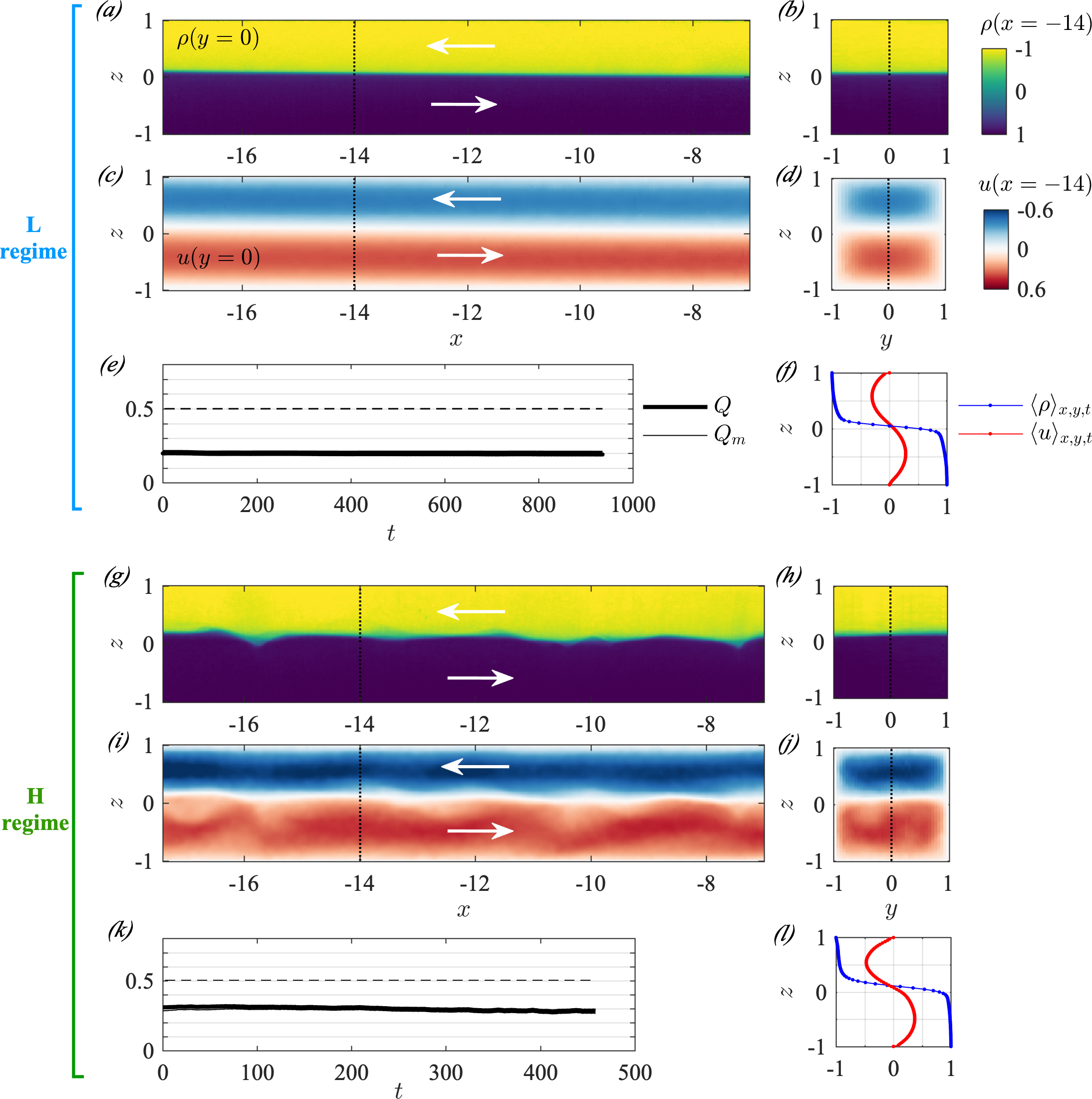
Figure 2: Comparative visualisations of a typical (a-f) L flow ($\theta=2^{\circ}$, $Re=398$) and (g-l) H flow ($\theta=1^{\circ}$, $Re=1455$). The I and T regimes are shown in figure 3. The L and H data correspond respectively to experiments L1 and H1 listed in table LABEL:tab:3d-3c-expts (discussed later). For each experiment, we plot the density field $\rho$ and streamwise velocity field $u$ in (a,c,g,i) the vertical mid-plane of the volume $y=0$, and in (b,d,h,j) the arbitrary cross-sectional plane $x=-14$, all for a single arbitrary temporal snapshot: $t=150$ in (a-d), and $t=261$ in (g-j). Colour bars are identical for all plots showing density or velocity and are thus not repeated. Dotted vertical lines in the $y=0$ plane (a,c,g,i) indicate the location of the $x=-14$ plane in (b,d,h,j) and conversely. White arrows indicate the direction of the flow in each layer (in agreement with the notation of § 2.1 and figure 1). In addition, we plot for each experiment: (e,k) the temporal evolution of the volume flux $Q(t)$ and mass flux $Q_{m}(t)$ (the dashed line is the hydraulic limit $Q=0.5$); and (f,l) the mean vertical density and streamwise velocity profiles (the dot symbols indicate the vertical resolution of the data).

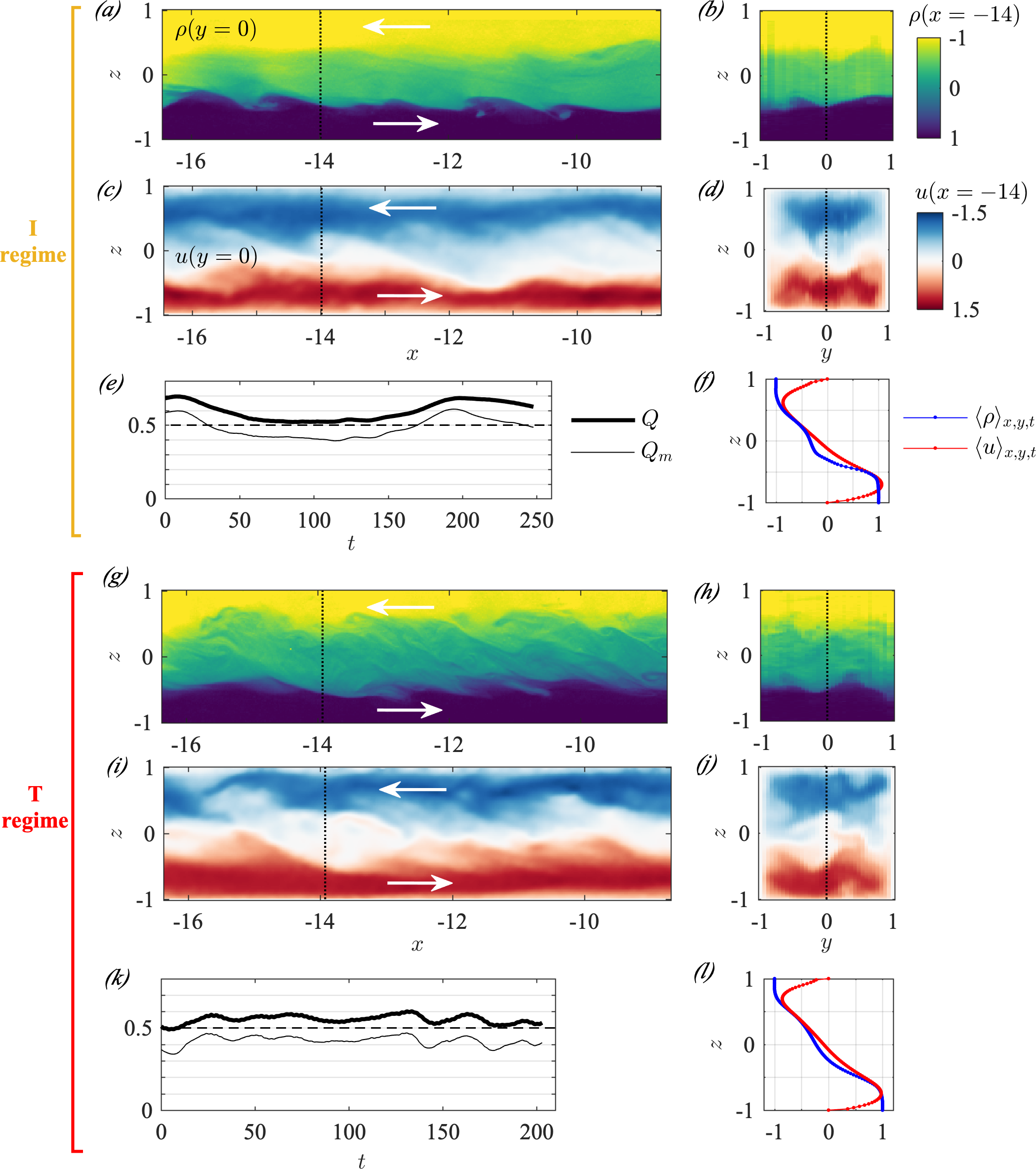
Figure 3: Comparative visualisations of a typical (a-f) I flow ($\theta=6^{\circ}$, $Re=777$) and (g-l) T flow ($\theta=6^{\circ}$, $Re=1256$), corresponding respectively to experiments I4 and T2 of table LABEL:tab:3d-3c-expts (discussed later). The legend is identical to that of figure 2, except for the temporal snapshots used here: $t=55$ in (a-d) and $t=168$ in (g-j).

We observe that the L and H flows have a sharp density interface with a tanh-like vertical profile (figure 2(a,b,f,g,h,l)), while the I and T flows have a mixing layer (figure 3(a,b,f,g,h,l)), i.e. a central layer in which the vertical density gradient is smaller than the values immediately above and below it as a result of turbulent mixing across the interface.

In the L and H regimes, the streamwise velocity profile has a sine-like vertical structure (figure 2(f,l)) indicative of fully-developed velocity boundary layers (expected when $Re\lesssim 50A=1500$). By contrast, in the I and T regimes, interfacial turbulence creates a region of approximately constant velocity gradient across the mixing layer and ‘pointier’ maxima that are pushed closer to the top and bottom walls (figure 3(f,l)) especially when turbulence is more intense and sustained in the T flow.

We also note that the L flow is largely (i) parallel, i.e. independent of the streamwise direction $x$, except for a very slight downward slope of the interface typical of such flows (discussed later in § LABEL:sec:two-layer-model); (ii) steady in time; (iii) symmetric about the $y=0$ and $z=0$ planes. By contrast, the H flow breaks the $x$- and $t$-invariance with a set of travelling, symmetric Holmboe waves distorting the density and velocity interfaces in a characteristic ‘cusp’-like pattern and in a quasi-periodic fashion (these ‘confined Holmboe waves’ were the focus of LPZCDL18). In addition, complex three-dimensional wave motions in the velocity field break the $y=0$ and $z=0$ symmetries (figure 2(i,j)).

In the I and T flows, the departure from both the $x,t$ invariances and the $y,z=0$ symmetries at any instant in time is even greater, owing to large, three-dimensional turbulent fluctuations (figure 3). Based on the deflections in the position of the density and velocity interfaces, the spatial scales of these fluctuations, and the amplitude of the temporal fluctuations in the $Q(t)$ and $Q_{m}(t)$ time-series, it is tempting to classify the L and H flows in one group based on their similarity, and the I and T regimes in a different group. The $\textsf{L}-\textsf{H}$ flows have lower volume and mass flux, which are equal in the absence of mixing ($Q_{m}\approx Q\approx 0.2-0.3$), while the $\textsf{I}-\textsf{T}$ flows have higher fluxes and significant mixing ($Q_{m}\approx 0.4-0.5<Q\approx 0.5-0.6$, close to the hydraulic limit).

Large temporal fluctuations in both $Q$ and $Q_{m}$ are observed in the I and T regimes, but I flows tend to exhibit a component with longer pseudo-period associated with oscillations between laminar and turbulent events (sometimes in a quasi-periodic fashion with period $O(100$ ATU$)$). This is visible in the I flow here (figure 3(e)): the start of a turbulent event (shown here in the snapshots figure 3(a-d) at $t=55$) follows the instability of an accelerating, largely laminar, three-layer flow. A peak in the volume flux at $t\approx 10$ triggered large-amplitude waves at both density interfaces which started overturning at $t\approx 40$ and initiated a turbulent event slowing down the flow (decreasing $Q$ and $Q_{m}$). Relaminarisation followed at $t\approx 130$ (increasing $Q$ and $Q_{m}$), and another cycle started (note that only one cycle was recorded here).

The basic characteristics of flow regimes described above are summarised in table 1.

	L	H	I	T
Invariance in $x,t$	$\checkmark$	$\sim$	$\times$	$\times$
Symmetry about $y,z=0$	$\checkmark$	$\sim$	$\times$	$\times$
Large $Q,Q_{m}\approx 0.5$	$\times$	$\times$	$\checkmark$	$\checkmark$
Interfacial mixing	$\times$	$\times$	$\checkmark$	$\checkmark$
Small spatial scales	$\times$	$\sim$	$\checkmark$	$\checkmark$
Laminar-turbulent periodicity	$\times$	$\times$	$\checkmark$	$\times$

Table 1: Basic characteristics of flow regimes inferred from figures 2-3. Symbol $\sim$ indicates a relatively small effect.

2.3 Regime diagram and previous studies

2.3.1 Regime diagram

The map of flow regimes L, H, I, T  in the $\theta-Re$ plane of input parameters is shown in figure 4. This regime diagram features a total of 360 points, corresponding to the qualitative identification of regimes for 360 $(\theta,Re)$ couples. Out of these, 312 were determined from shadowgraph observations (§ 2.2.1) as in ML14, 35 were determined from 3D-3C experiments (§ 2.2.3), and 13 from simpler planar PIV and PLIF measurements (two-dimensional, two-component, in the $y=0$ plane) that were carried out before the 3D-3C system was operational (these measurements are not discussed in this paper).

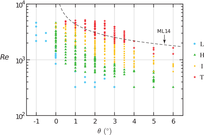
Figure 4: Regime diagram in the $(\theta,\,Re)$ plane of non-dimensional input parameters totalling 360 data points. In dashed, the $\textsf{I}\rightarrow\textsf{T}$ transition curve obtained from experiments in a larger duct by ML14 (see § 2.3.2).

We observe that the L, H, I  and T  regimes largely occupy distinct regions of the $\theta-Re$ plane, with little overlap. We refer to the boundaries between each regime respectively as the $\textsf{L}\rightarrow\textsf{H}$, $\textsf{H}\rightarrow\textsf{I}$, and $\textsf{I}\rightarrow\textsf{T}$ transitions, which can be described by simple open curves in the $\theta-Re$ plane. To fix ideas, we may formally define a ‘regime function’ $\mathrm{reg}$ taking arbitrary but increasing values such as

$$\mathrm{reg}\equiv 1\ \textrm{for}\ \textsf{L},\ \ 2\ \textrm{for}\ \textsf{H},\ \ 3\ \textrm{for}\ \textsf{I},\ \ 4\ \textrm{for}\ \textsf{T}.$$ (13)

Finding the scaling of flow transitions is equivalent to finding the functional dependence of the regime function with respect to the two input parameters varied in this paper: $\mathrm{reg}(\theta,Re)$. Such ‘transition curves’ can then be described, for example, by the equations $\mathrm{reg}=1.5,\,2.5,\,3.5$.

Sufficiently far from the transitions curves, the flow regime is a repeatable characteristic of the experiment (and of the underlying dynamical system) for a choice of input parameters $(\theta,\,Re)$. The slight overlap between regimes near the transitions is interesting, and may be explained by two potential reasons:

1. the flow regime may not be a reproducible characteristic of the experiment (and of the underlying dynamical system) near the transitions due to its sensitivity to flow parameters, and/or to initial conditions (the initial transients resulting from the way the experiment is started, which cannot be controlled accurately);

2. the qualitative (visual) identification of flow regimes, i.e. the very definition of ‘flow regime’ is not appropriate near the transitions (i.e. not fine or consistent enough) to classify the flow into the four discrete categories of ML14.

Note that throughout this paper, we use the term ‘regime transition’ to refer to the change in the qualitative long-term (asymptotic) dynamics of the flow caused by changes in the input parameters. Although mathematically such behaviour is typically referred to as a bifurcation, we chose to avoid this term in this paper since we do not prove nor imply that the underlying dynamical system indeed exhibits strict bifurcations. This question is interesting but outside the scope of this paper.

2.3.2 meyer_stratified_2014

The regime diagram in figure 4 complements that of ML14 (their figure 5). ML14 plotted it in the $\theta-\Delta\rho/(2\rho_{0})$ plane) for 93 experiments using a larger duct ($H=100$ mm vs $45$ mm) of the same aspect ratio ($A=30$). They sought an equation for the transition curves by arguing that, because of the presence of hydraulic controls (§ 2.1), the kinetic energy in the flow was bounded by the scaling $(\Delta U)^{2}\sim g^{\prime}H$ (see (4) and (5)) and thus it could not increase even in the presence of gravitational forcing when $\theta>0^{\circ}$. The dimensional ‘excess kinetic energy’ $g^{\prime}L\sin\theta$, gained by conversion from potential energy by the fluid travelling a distance $L$ along the duct in the streawise field of gravity $g^{\prime}\sin\theta>0$, thus has to be dissipated by increased wave activity or turbulence. They non-dimensionalised this excess kinetic energy by $(\nu/H)^{2}$, thus forming the following Grashof number

$$Gr\equiv\frac{g^{\prime}L\sin\theta}{(\nu/H)^{2}}=4A\sin\theta Re^{2},$$ (14)

where the first equality is their definition and the second equality uses our notation. They found reasonable agreement between this scaling in $\sin\theta Re^{2}$ (using two different aspect ratios $A=15,\,30$) and suggested the empirical equation $Gr=4\times 10^{7}$ for the $\textsf{I}\rightarrow\textsf{T}$ transition curve (see their figure 8).

Their proposed $\textsf{I}\rightarrow\textsf{T}$ transition curve is reproduced in dashed black in figure 4 (identified by the ‘ML14’ arrow) to show that the agreement in our geometry (smaller duct) is less convincing. The ML14 curve lies entirely in the T  region (i.e. it is ‘too high’) and the discrepancy is particularly apparent at higher angles $\theta\gtrsim 4^{\circ}$ (which were not considered by ML14), suggesting that their proposed ‘$\sin\theta Re^{2}$ scaling’ of transitions may not be universal.

2.3.3 macagno_interfacial_1961

macagno_interfacial_1961 also mapped these same four regimes in a two-dimensional space (see their figure 8). However, instead of two input parameters such as $\theta$ and $Re$, they used a Froude number and a Reynolds number based on measured values of the actual (output) $\Delta U$ and of the vertical distance between the two maxima of $|u|$ (depth of the shear layer). They varied the tilt angle $\theta$ in non-trivial ways, sometimes during an experiment, in order to obtain target values of $\Delta U$ and therefore better control $Re$, and did not appear to realise the presence and importance of hydraulic controls (in fact, they may have disturbed them by their use of splitter plates at the ends of the duct). They recognised the importance of $Re$ in regime transitions, but not that of $\theta$, and were thus unable to propose a convincing physical model to substantiate the transitions.

2.3.4 kiel_buoyancy_1991

The third most relevant experimental study of regime transitions in the SID experiment is the (unpublished) PhD thesis of kiel_buoyancy_1991 (like most of the literature, he was not aware of macagno_interfacial_1961). Kiel proposed a heuristic scaling based on a ‘geometric Richardson number’ $Ri_{G}\equiv(4A\tan\theta+16/9)^{-1}$ (using our notation). We interpret the parameter $Ri_{G}^{-1}$ as the non-dimensionalisation of the ‘excess kinetic energy’ $g^{\prime}L\sin\theta$ of ML14 by the actual kinetic energy of the hydraulically-controlled flow $(\Delta U)^{2}=g^{\prime}H$, i.e. $Ri_{G}^{-1}\sim g^{\prime}L\sin\theta/(g^{\prime}H)=A\sin\theta$ (disregarding the additive constant $16/9$). Hence, when the excess energy to be dissipated becomes large compared with the maximum kinetic energy of the flow (high $Ri_{G}^{-1}$), transition to turbulence is expected.

Contrary to macagno_interfacial_1961, kiel_buoyancy_1991 only focused on the importance of $\theta$ on regime transitions, ignoring $Re$ which he (incorrectly) assumed large enough for viscous effects to be ignored. Although Kiel did use large $Re$ (of order $10^{4}$) using ducts of dimensions similar to that of ML14, the observations of ML14 at similar $Re$ highlighted the importance of the $Re$ scaling, which we substantiate in this paper. Consequently, his $Ri_{G}$ criterion, based a non-dimensionalisation of the excess kinetic energy by the velocity scale $\Delta U$ – although apparently more physical than the somewhat arbitrary velocity scale $\nu/H$ of ML14 – is fundamentally incapable of predicting regime transitions.

2.4 Aim and outline

To summarise, we have seen that regime transitions in the SID depend on at least two input parameters: $\theta$ and $Re$. The first two pioneering attempts to understand the transitions that we are aware of (macagno_interfacial_1961; kiel_buoyancy_1991) each ignored one of them, proposing heuristic scalings based on (respectively) either $Re$ or $\theta$. More recently, ML14 correctly identified the $\theta-Re$ dependence, understood the consequence of hydraulic controls, and proposed a transition scaling following $Gr\sim\sin\theta Re^{2}=$ const. (see (14)). This scaling was based on heuristic arguments of ‘excess kinetic energy’, which, as we will show this paper, are essentially correct but can be made more specific. However, the non-dimensionalisation by the square velocity scale $(\nu/H)^{2}$ leading to the Grashof number $Gr$ is not justifiable by physical principles, nor is the value $Gr=4\times 10^{7}$ for the $\textsf{I}\rightarrow\textsf{T}$ transition. In addition, although their $\sin\theta Re^{2}$ transition scaling agreed well with their data, it does not appear to agree with our more recent and comprehensive data obtained in a smaller duct (figure 4). We believe that the above points motivate the need for a revised scaling based on sound physical principles that are verified experimentally.

The qualitative classification into four discrete regimes introduced by macagno_interfacial_1961 and ML14 is an important first step in the study of the dynamics of sustained stratified shear flows. The presence or absence of interfacial waves, of small-scale structures indicative of turbulence, of spatio-temporal intermittency can all easily be picked by the eye using simple shadowgraph visualisation or dye visualisation (PLIF) and provide valuable ‘order one’ information about the asymptotic (long-term, i.e. over hundreds of ATU) behaviour of the underlying dynamical system. Our novel volumetric 3D-3C measurements now allow us to complement these qualitative observations with quantitative analyses of flows in each regime to investigate in more details their steady-state (asymptotic) dynamical equilibria.

We thus reformulate the aim of this paper introduced in § 1 more specifically as: finding a quantitative, physical basis explaining the different qualitative asymptotic behaviours of such sustained stratified shear flows (i.e. the ‘flow regimes’). Analysis of the past literature and our experimental observations suggest that the two leading non-dimensional input parameters of interest are $\theta$ and $Re$ ($A$ and $Sc$ playing lesser roles), hence we shall focus on them exclusively and seek transition curves of the form $\mathrm{reg}(\theta,Re)=$ const.

To tackle this aim, the rest of the paper is organised as follows. In § 3, we derive from first principles a framework of energy budget analyses suited to our 3D-3C measurements. In § LABEL:sec:exp-validation, we compare predictions for regime transition based on this framework to our experimental data. In § LABEL:sec:3d, we further develop this framework and the analysis of experimental data to get a deeper understanding of the relation between flow regimes and energetics. Finally, we summarise our findings and suggest future directions in § LABEL:sec:ccl.

3 The energetics framework

In this section we introduce the theoretical framework to analyse the energetics of SID flows. We start by deriving the time evolution equations for the kinetic energy and potential energy, first as local quantities in § 3.1, and then averaged in a control volume in § LABEL:sec:avg-budgets. To jump to the result of this section, see equations (LABEL:dKdt-final) and (LABEL:dPdt-final) and figure LABEL:fig:energetics-1. We then estimate the transfer terms between kinetic and potential energies and simplify the budgets in § LABEL:sec:estimations. Finally, we focus on one particular simplified budget in order to formulate an hypothesis regarding the regime transitions in § LABEL:sec:implications.

3.1 Local energy budgets

The governing equations on which all subsequent analyses are based are the incompressible Navier-Stokes equation under the Boussinesq approximation coupled to the advection-diffusion of density. Under the notation and conventions adopted in § 2.1, they take the following non-dimensional form ∇⋅u&= 0, eq-motion-1
_t u+ u⋅∇u= -∇p + Ri   ( -cosθ