Conductivity and capacitance of streamers in avalanche model for streamer propagation in dielectric liquids

Abstract

Propagation of positive streamers in dielectric liquids, modeled by the electron avalanche mechanism, is simulated in a needle–plane gap. The streamer is modeled as an RC-circuit where the channel is a resistor and the extremities of the streamer have a capacitance towards the plane. The addition of the RC-model introduces a time constant to the propagation model. Increase in capacitance as a streamer branch propagates reduces its potential, while conduction through the streamer channel increases its potential, as a function of the time constant of the RC-system. Streamer branching also increases the capacitance and decreases the potential of the branches. If the electric field within the streamer channel exceeds a threshold, a breakdown occurs in the channel, and the potential of the streamer is equalized with the needle electrode. This is interpreted as a re-illumination. According to this model, a low conductive streamer branch can propagate some distance before its potential is reduced to below the propagation threshold, and then the RC time constant controls the streamer propagation speed. Channel breakdowns, or re-illuminations, are less frequent when the channels are conductive and more frequent for more branched streamers.

Keywords: Streamer, Simulation Model, Dielectric Liquid, Conductivity, Capacitive Model,

1 Introduction

When dielectric liquids are exposed to a sufficiently strong electric field, partial discharges occur and a gaseous channel called a streamer is formed. The many characteristics of streamers, such as shape, propagation speed, inception voltage, breakdown voltage, current, and charge are described by numerous experiments performed throughout the last half century for various liquids and different experimental setups [1, 2, 3, 4, 5, 6]. A streamer bridging the gap between two electrodes can cause an electric discharge, and a better understanding of the mechanisms governing the inception and the propagation of streamers is essential for the production of e.g. better power transformers and the prevention of failure in such equipment [7].

Simulating a low temperature plasma in contact with a liquid is a challenge in itself [8]. For a propagating streamer, phase change and moving boundaries complicates the problem further and simplifications are therefore required. The finite element method has been used in models simulating streamer breakdown through charge generation and charge transport [9, 10], even incorporating phase change [11]. However, the first simulations of streamer breakdown in liquids applied Monte Carlo methods on a lattice [12], and have since been expanded, for instance by including conductivity [13]. Another model use the electric network model to calculate the electric field in front of the streamer, which is used to evaluate the possibility for streamer growth or branching [14].

For positive streamers in non-polar liquids, it is common to define four propagation modes based on their propagation speed, ranging from around $0.1\text{\,}\mathrm{km}\text{\,}{\mathrm{s}}^{-1}$ for the 1st mode and exceeding $100\text{\,}\mathrm{km}\text{\,}{\mathrm{s}}^{-1}$ for the 4th mode. 2nd mode streamers propagate at speeds of some $\mathrm{km}\text{\,}{\mathrm{s}}^{-1}$ creating a branching filamentary structure that can lead to a breakdown if the applied voltage is sufficiently high [15].

Our previous work describes a model for propagation of 2nd mode positive streamers in dielectric liquids governed by electron avalanches [16, 17]. According to the model, electron avalanches can be important for streamer propagation, but the results also showed a relatively low propagation speed and a low degree of branching. The streamer channel was represented by a fixed electric field within the channel between the needle electrode and the extremities of the streamer. The model focuses on the phenomena occurring in the high electric field in front of a streamer, assuming these are the main contributors to the propagation. However, processes in the channel may be important for the electric field at the streamer extremities, which is why it is addressed in this study. Here, the channel is included by considering its conductivity as well as capacitance between the streamer and the plane.

2 Simulation model and theory

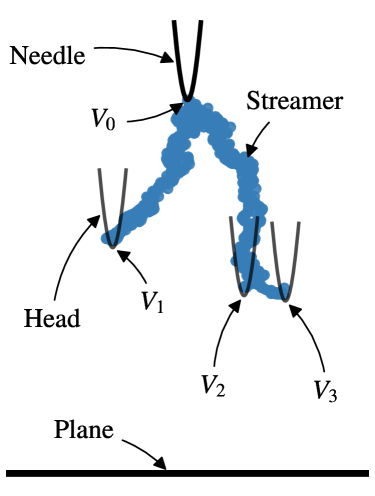
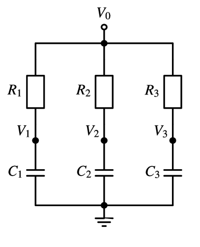
Figure 1: (left) Illustration of the needle electrode, a branched streamer, and three streamer heads above a planar electrode, and (right) the equivalent RC-circuit.

2.1 Electron avalanche model

We simulate streamer propagation in a liquid-filled needle–plane gap. The needle is represented by a hyperboloid and the streamer is represented by a number of hyperboloidal streamer heads, see figure 1. Each hyperboloid $i$ has a potential $V_{i}$ and an electric field $\bm{E}_{i}$. A potential $V_{0}$ is applied to the needle when the simulation begins. Since we here are interested in propagation rather than initiation of streamers, a square wave with infinite risetime is applied. The potential of each streamer head $V_{i}$ is dependent on the potential and capacitance of the streamer (see section 2.3), and changes with time (see section 2.4). The method of calculation gives a drop in potential between the needle tip and the streamer tip, which is an important feature of the model. The Laplacian electric field $\bm{E}_{i}$ is dependent on the potential $V_{i}$ and calculated using the hyperbole approximation [17]. The potential and electric field at a given position $\bm{r}$ is given by the superposition principle,

$$V(\bm{r})=\sum\limits_{i}k_{i}V_{i}(\bm{r})\,\quad\text{and}\quad\bm{E}(\bm{r})=\sum\limits_{i}k_{i}\bm{E}_{i}(\bm{r})\,,$$ (1)

where the electrostatic shielding coefficients $k_{i}$ are optimized such that $V(\bm{r}_{i})=V_{i}(\bm{r}_{i})$, i.e. the superposition of potentials gives the correct potential at the tip of each head. Each head with $k_{i}$ lower than $k_{\textrm{c}}$ (shielding threshold) is removed and heads closer than $d_{\textrm{m}}$ (head merge threshold) are merged [17]. A number of anions, given by the anion number density $n_{\textrm{ion}}$, is placed at random positions in the liquid volume surrounding the streamer. Anions are considered as sources of seed electrons, which can turn into electron avalanches if the electric field is sufficiently high. The number of electrons $N_{\textrm{e}}=\exp(Q_{\textrm{e}})$ in an avalanche increases each simulation time step $\Delta{}t$. The change in $Q_{\textrm{e}}=\ln N_{\textrm{e}}$, $\Delta Q_{\textrm{e}}$, is given by

$$\Delta{}Q_{\textrm{e}}=E\,\mu_{\textrm{e}}\,\alpha_{\textrm{m}}\exp\!\left(-\frac{E_{\alpha}}{E}\right)\Delta{}t\,,$$ (2)

where $\mu_{\textrm{e}}$ is the electron mobility, and $\alpha_{\textrm{m}}$ and $E_{\alpha}$ are experimentally estimated parameters. An avalanche is considered “critical” if $Q_{\textrm{e}}$ exceeds a threshold $Q_{\textrm{c}}$ (Townsend–meek criterion, $N_{\textrm{e}}=\exp Q_{\textrm{e}}>\exp Q_{\textrm{c}}$). Critical avalanches are removed, replaced by a new streamer head. The tip of the new streamer head is positioned where the avalanche became critical, and this way, the streamer grows [17].

The potential of the new head was set assuming a fixed electric field $E_{\textrm{s}}$ in the streamer channel [17], but here the model is extended so that the potential is instead calculated by considering an RC-circuit.

2.2 RC-circuit analogy for streamers

A simple RC-circuit is composed of a resistor and a capacitor connected in series. When voltage is applied, the capacitor is charged and its potential increases as a function of time. The time constant $\tau$ of an RC-circuit is

$$\tau=RC\,,$$ (3)

where $R$ is the resistance and $C$ is the capacitance. Similarly, the streamer channel is a conductor with an associated resistance, and the gap between the streamer and the opposing electrode is associated with a capacitance, see figure 1. This is a reasonable assumption when modeling a dielectric liquid where the dielectric relaxation time is long compared to the duration of a streamer breakdown [6].

For a given streamer length $\ell$, cross-section $A$, and conductance $\sigma$, the resistance is given by

$$R=\frac{\ell}{A\sigma}\,.$$ (4)

The resistance is proportional to the streamer length, calculated as the straight distance from the needle to the streamer head. Also $A$ and $\sigma$ may change during propagation. For instance, during a re-illumination, one or more of the streamer channels emit light [18]. This is likely the result of the buildup of a strong electric field within the channel, causing a a gas discharge within the channel, increasing $\sigma$ and lowering $R$ significantly [19]. It seems reasonable to assume that the resistance is reduced for some time after a re-illumination, however, measurements shows just a brief spike in the current, typically lasting about $10\text{\,}\mathrm{ns}$ [18], which is consistent with the time scale for charge relaxation of ions in the channel [20].

The total charge of a streamer can be found by integrating the current and is in the range of $\mathrm{nC}$ to $\mathrm{\SIUnitSymbolMicro C}$ [21, 22, 6]. The “capacitance” of the streamer can be approximated by considering the streamer to be a conducting half-sphere (slow and fine-branched modes) or a conducting cylinder (fast and single-branched modes), which also enables the calculation of the field in front of the streamer [3, 21, 23]. We associate each streamer head with the capacitance between itself and the planar electrode, as illustrated in figure 1. The capacitance then depends on the geometry of the gap between them, and an increase in streamer heads increases the total capacitance of the streamer. The capacitance for a hyperbole is applied for the avalanche model, while models for a sphere over a plane and a parallel plate capacitor are included here as limiting cases.

The capacitance of a hyperbole is approximated in A by integrating the charge on the planar electrode,

$$C_{\textsc{H}}(z)\propto\left({\ln\frac{4z+2r_{\textrm{p}}}{r_{\textrm{p}}}}\right)^{-1}\,,$$ (5)

where $r_{\textrm{p}}$ is the tip curvature of the hyperboloid and $z$ is the distance to the plane. The capacitance of a parallel plane capacitor is

$$C_{\textsc{P}}(z)\propto\frac{1}{z}\,,$$ (6)

where $z$ is the distance between the planes, and the capacitance for a sphere above a plane is [24]

$$C_{\textsc{S}}(z)\propto r_{\textrm{p}}\left(1+\frac{1}{2}\ln\left(1+\frac{r_{\textrm{p}}}{z}\right)\right)\,,$$ (7)

where $r_{\textrm{p}}$ is the radius of the sphere. The difference in capacitance for the three models is substantial, see figure 2. A single sphere does not take a conducting channel into account, and this is the reason why its capacitance does not change significantly before $z$ is about ten times $r_{\textrm{p}}$. Conversely, for the planar model, the capacitance grows rapidly as it doubles every time $z$ is halved, but assuming parallel planes is considered an extreme case.

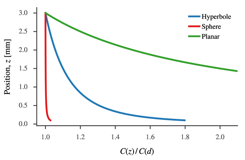
Figure 2: The three proposed models for capacitance as a function of the position in gap.

To test the impact of the variation in streamer channel conductivity and capacitance on the streamer propagation we will use a simplified model, where electrical breakdown within the channel is also included. Each streamer head is assigned a time constant $\tau$, which is split into several contributions,

$$\tau=fgh\tau_{0}\quad\text{with}\quad\tau_{0}=\frac{Cd}{A\sigma}\,,$$ (8)

where $d$ is the gap distance. The contributions

$$f=\frac{\ell}{d}\,,\quad g=\frac{C(z)}{C(d)}\,,\quad\text{and}\quad h=\Theta(E_{\textrm{bd}}-E_{\textrm{s}})\,,$$ (9)

represent change in resistance in the channel ($f$), capacitance between the streamer head and the plane ($g$), and the breakdown in the channel ($h$), respectively. The Heaviside step function $\Theta$ is zero when the electric field in the channel is larger than the breakdown threshold ($E_{\textrm{s}}>E_{\textrm{bd}}$) and one otherwise. When a breakdown in the channel occurs $\Theta=0$, giving $\tau=0$, and thus the potential at the streamer head is instantly relaxed to the potential of the needle. We therefore assume that breakdowns in the channel is the cause of re-illuminations. Since the heads are individually connected to the needle, a breakdown only affects one channel.

Having $\tau$ longer or shorter than the streamer propagation time implies relatively low or high conductivity, respectively. Since the contributions $f$, $g$, and $h$ are on the order of magnitude 1 for most parts of the gap, the same is true for $\tau_{0}$ (although $\tau_{0}=R(0)C(d)$ does not have a physical interpretation). Throughout the simulations, an increase in $\tau_{0}$ is considered to arise from a decrease in the channel conductivity $\sigma$, and vice-versa. The influence of channel expansion (increasing $A$), is included in the discussion in section 5, as well as evaluation of conductivity from $\tau_{0}$.

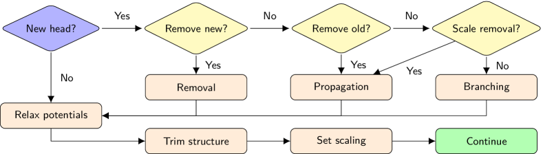
Figure 3: Algorithm for updating the streamer structure. “Collision” and “merging” checks decides whether the head should be removed immediately. The same checks are then performed to see if the addition of the head causes an existing head to be removed. Then, a “scale removal” check is performed at equipotential. See text in section 2.4 for details on these checks. If the new head is not removed and a check finds a head to remove, the new head is a “propagating” head and its potential is set by 10. Else, it is a “branching head” and its potential is set by 12, which changes the potential of an existing streamer head as well. All potentials are then relaxed according to 13. Finally, the structure is trimmed by checking “collision”, “merging” and “scale”, and the correct scale is set, as described in [17].

2.3 Electrical potential of new streamer heads

The potential of a new head $m$ is dependent on the closest streamer head $n$ only. This is an approximation compared with using an electric network model for the streamer [14] and in contrast to our previous model using fixed electric field in the streamer channel [17]. Two different cases are implemented, depending on whether the new head can cause a branching event or not (see details in section 2.4 and figure 3). If the new head is not considered to be a new branch its potential is calculated assuming charge transfer from $n$ to $m$,

$$V_{m}=V_{n}\frac{C_{n}}{C_{m}}\,.$$ (10)

Secondly, the potential for a branching head is calculated by sharing the charge between $n$ and $m$, reducing the potential of $n$ as well. Isolating the two heads from the rest of the system, the total charge is $Q=V_{n}C_{n}$, and this charge should be divided in such a way that the heads obtain the same potential, $V(\bm{r}_{m})=V(\bm{r}_{n})$, using 1 for both $m$ and $n$. Introducing $M_{ij}=V_{j}(\bm{r}_{i})/V_{j}(\bm{r}_{j})$, 1 is simplified as

$$V_{i}(\bm{r}_{i})=\sum\limits_{j}M_{ij}k_{j}V_{j}(\bm{r}_{j})\;\Rightarrow\;1=\sum\limits_{j}M_{ij}k_{j}\,,$$ (11)

when all $V_{i}(\bm{r}_{i})$ are equal. The coefficients $k_{j}$ are obtained by NNLS-optimization [17], like the potential shielding coefficients. Finally, the potential for both $m$ and $n$ is calculated as

$$V_{m}(\bm{r}_{m})=\frac{Q}{\sum k_{i}C_{i}}\,.$$ (12)

In the case where one $k_{i}$ is close to unity and the other is close to zero, the result resembles 10, however, $\sum k_{i}\geq 1$, so the potential will drop when the capacitance of the new head is similar to or larger than its neighbor. The potential of a new head could also have been set to the potential at its position calculated before it is added, but that probably overestimates the reduction in potential, since the avalanche itself distorts the electric field and since transfer of charge from neighboring heads is faster than from the needle.

2.4 Updating the streamer

In [17], critical avalanches are replaced by new streamer heads and added to the streamer. Any head within another head has “collided” with the streamer and is removed. If two heads are too close to each other they are “merged”, implying that the one closest to the plane is kept and the other one is removed. Also, the potential shielding coefficients are calculated and any head with a low coefficient is removed, “scale removal”. Finally, the shielding coefficients are set.

The algorithm is now changed, see figure 3 (replacing the block labeled “Streamer” in figure 5 in [17]). New heads are either removed, or classified as “propagating” or “branching”, and their potential is set using 10 or 12. If a head can be added without causing another to be removed, it can cause a branching event, else it represents propagation of the streamer. The addition of one extra head is by itself not sufficient for streamer branching, often there are several heads within one propagating branch. Branching occurs through a process of adding new heads to opposing sides of a cluster of heads while removing the heads in the center (cf. figure 28 in [17]). With this approach, branching follows as a consequence of propagation, contrary to models in which streamers propagate by adding branches [12, 14] or models which rely on inhomogeneities [10].

The difference in potential between each head $V_{i}$ and the needle $V_{0}$ is first found and then reduced,

$$\Delta V_{i}=V_{0}-V_{i}(\bm{r}_{i})\;\rightarrow\;V_{i}(\bm{r}_{i})=V_{0}-\Delta V_{i}\,e^{-\Delta t/\tau_{i}}\,.$$ (13)

where the time constant of each head $\tau_{i}$ is calculated by 8. Finally, the streamer structure is trimmed (collision, merge and scale removal) and the potential scaling is optimized as described in [17]. Note trimming and rescaling is performed to remove heads lagging behind and to ensure correct potential at each streamer head, however, it does not preserve charge and capacitance. For this reason, we do not calculate the total charge or capacitance of the streamer.

3 Single channel streamer at constant speed

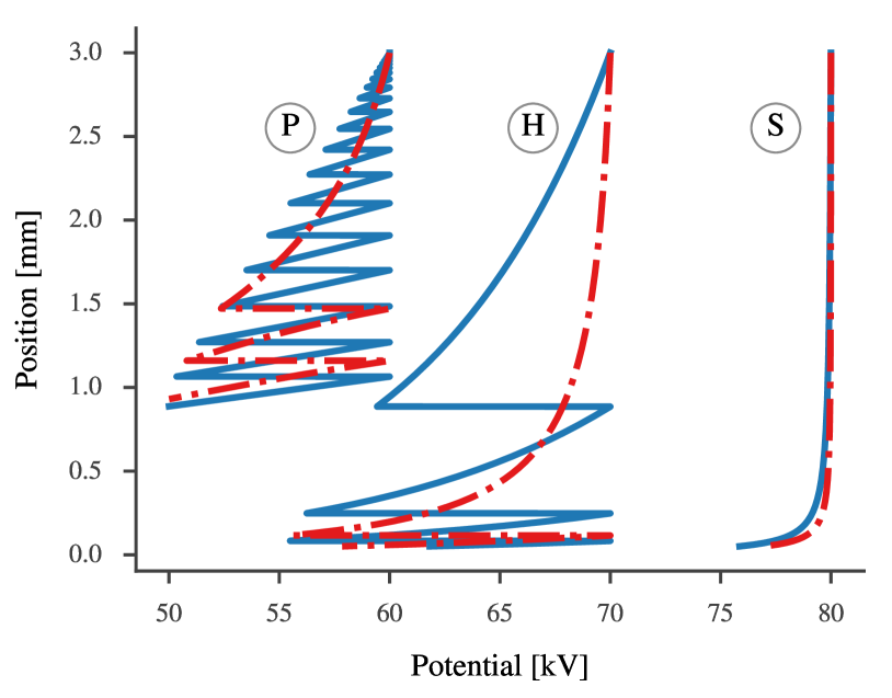
Figure 4: Potential of single head propagating at constant speed, starting at at different potentials for different capacitance models: (P)lane, (H)yperbole, and (S)phere, Time constants $\tau_{0}=$0.1\text{\,}\mathrm{\SIUnitSymbolMicro s}$$ (dashed red) and $\tau_{0}=$10\text{\,}\mathrm{\SIUnitSymbolMicro s}$$ (solid blue), and breakdown in channel at $E_{\textrm{bd}}=$5\text{\,}\mathrm{kV}\text{\,}{\mathrm{mm}}^{-1}$$.

As a model system, a simplified numerical model is investigated by considering a streamer propagating as a single branch at constant speed. The parameters used are gap distance $d=$3\text{\,}\mathrm{mm}$$, propagation speed $v_{\textrm{p}}=$3\text{\,}\mathrm{km}\text{\,}{\mathrm{s}}^{-1}$$, tip radius $r_{\textrm{p}}=$6\text{\,}\mathrm{\SIUnitSymbolMicro m}$$, minimum propagation voltage $V_{\textrm{p}}=$50\text{\,}\mathrm{kV}$$, and breakdown in the channel at $E_{\textrm{bd}}=$5\text{\,}\mathrm{kV}\text{\,}{\mathrm{mm}}^{-1}$$. The time constant $\tau$ is modeled by 8 and 9 and the potential is calculated by 10.

The result of varying $\tau_{0}$ for the different capacitance models $g$, is shown in figure 4. When applying the sphere model in 7, the change in potential is small and the time constant has little influence, as expected based on figure 2. The potential changes faster with the hyperbole model in 5 and breakdown in the channel occurs in the final part of the gap. Decreasing $\tau_{0}$, i.e. increasing the conductivity, reduces the potential drop and delays the onset of breakdowns in the channel. This is similar for the plane model in 6, where rapid breakdowns at the start of the propagation are suppressed by decreasing $\tau_{0}$. The propagation for the plane model is stopped when the potential drops below $V_{\textrm{p}}$, which occurs at about the same position for both low and high $\tau_{0}$. Where the propagation stops depends on the capacitance model, the breakdown in channel threshold, the time constant, and the initial voltage $V_{0}$. A reduction of $V_{0}$ by $10\text{\,}\mathrm{kV}$ for the hyperbole model would have stopped these streamers as well, but the one with higher conduction would have propagated most of the gap, stopping close to the opposing electrode.

By assuming an initial capacitance $C={$0.1\text{\,}\mathrm{pF}$}$, the energy ($W=\frac{1}{2}CV^{2}=\frac{1}{2}Q^{2}C^{-1}$) of each streamer head in figure 4 is some hundred $\mathrm{\SIUnitSymbolMicro J}$. From figure 2, the capacitance of the hyperbole model increases by about 20 % during the first $2\text{\,}\mathrm{mm}$, which amounts to some tens of $\mathrm{\SIUnitSymbolMicro J}$, and more than approximately $5\text{\,}\mathrm{\SIUnitSymbolMicro J}\text{\,}{\mathrm{mm}}^{-1}$ required for propagation [25]. Just before the first breakdown for the low-conductivity “hyperbole streamer” in figure 4, there is a voltage difference of about $10\text{\,}\mathrm{kV}$. Given a $\tau$ of about $10\text{\,}\mathrm{\SIUnitSymbolMicro s}$ this equals a continuous current of about $100\text{\,}\mathrm{\SIUnitSymbolMicro A}$, while the first breakdown adds about a $\mathrm{nC}$ of charge. In comparison, the high-conductivity “hyperbole streamer” has a current of more than a $\mathrm{mA}$, sustaining the potential at the streamer head for the first part of the propagation. As such, the current and charge are comparable to experimental results [22].

4 Numerical simulation results

Table 1: Model parameter values.

Gap distance	$d_{\textrm{g}}$	$3.0\text{\,}\mathrm{mm}$
Needle curvature	$r_{\textrm{n}}$	$6.0\text{\,}\mathrm{\SIUnitSymbolMicro m}$
Streamer head curvature	$r_{\textrm{s}}$	$6.0\text{\,}\mathrm{\SIUnitSymbolMicro m}$
Scattering constant	$E_{\alpha}$	$1.9\text{\,}\mathrm{GV}\text{\,}{\mathrm{m}}^{-1}$
Max avalanche growth	$\alpha_{\textrm{m}}$	$130\text{\,}{\mathrm{\SIUnitSymbolMicro m}}^{-1}$
Meek constant	$Q_{\textrm{c}}$	$23\text{\,}$
Electron mobility	$\mu_{\textrm{e}}$	$45\text{\,}\mathrm{m}\mathrm{m}\mathrm{}{2}\mathrm{/}{\mathrm{V}\mathrm{s}}$
Anion number density	$n_{\textrm{ion}}$	$2e12\text{\,}\mathrm{/}\mathrm{m}\mathrm{}{3}$
Head merge threshold	$d_{\textrm{m}}$	$50\text{\,}\mathrm{\SIUnitSymbolMicro m}$
Shielding threshold	$k_{\textrm{c}}$	$0.10\text{\,}$
Simulation time step	$\Delta t$	$1.0\text{\,}\mathrm{ps}$

Positive streamers in cyclohexane are simulated in a needle-plane gap. Model parameters discussed in this work are given in table 1. The base parameters and their influence on the model were discussed in [17] and is therefore not repeated here. The values for $\alpha_{\textrm{m}}$ and $E_{\alpha}$ have been taken from [26] rather than [27], decreasing the propagation voltage from about $60\text{\,}\mathrm{kV}$ to about $40\text{\,}\mathrm{kV}$ [17], which is closer the experimentally estimated $33\text{\,}\mathrm{kV}$ [22]. Experimentally, the propagation voltage is determined from either the streamer shape, the measured current, or interpolation of the propagation length  [28, 22]. For our simulations investigating propagation, however, the minimum requirement is simply a streamer length of 25 % of the gap, since most simulated non-breakdown streamers stop within the first few hundred $\mathrm{\SIUnitSymbolMicro m}$ [17]. In the updated model, the field in the streamer $E_{\textrm{s}}$ is not fixed but calculated by applying the RC-model described here. The influence of the conduction and breakdown in the streamer channel is investigated by changing values for $\tau_{0}$ and $E_{\textrm{bd}}$. Interesting values for $\tau_{0}$ are within some orders of magnitude of the propagation time for a streamer. The interpretation in terms of streamer radius and conductivity is discussed in the next section. For $E_{\textrm{bd}}$ to affect streamers in a $\mathrm{m}\mathrm{m}$-sized gap, minimum some $\mathrm{k}\mathrm{V}\mathrm{/}\mathrm{m}\mathrm{m}$ are needed, however, the average electric field within the streamer $E_{\textrm{s}}$ is dependent on both $\tau_{0}$ and $E_{\textrm{bd}}$. In section 3, we indicate how conductivity and capacitance influence the potential of a streamer propagating at constant speed. In this section, however, only the hyperbole model for capacitance is used. Furthermore, the propagation speed depends on the potential in the simulation model [17], and allowing multiple heads increases the total capacitance of the streamer, which gives a drop in potential when an extra streamer head is added.

The simulations presented in figure 6 have equal voltage and equal initial anion placement (initial random number). The streamers are visualized in figure 6(a), showing some increase in thickness and decrease in branching when the conductivity increases, however, their propagation speeds in figure 6(b) clearly differ. The propagation speed is mainly influenced by the number of streamer heads and the potential of the streamer heads [17]. Figure 6(c) shows that when there is no breakdown in the channel, and the conductivity is low, i.e. $\tau_{0}$ is high compared to the gap distance and propagation speed, the potential is reduced as the streamer propagates. For some short distances, the slow potential reduction is similar to the results in figure 4, however, when an extra head is added to the streamer (possible branching) there is a distinct reduction in the potential of some $\mathrm{kV}$. Increased conductivity increases the speed and average potential of the streamers in figure 6(c). At $\tau_{0}=$e-6\text{\,}\mathrm{s}$$, a single branch may gain potential during propagation while branching reduces the overall potential. This is reasonable since $\tau_{0}$ is about a tenth of the time to cross the gap, see figure 6(b). By further increasing the conductivity (decreasing $\tau_{0}$ to $e-8\text{\,}\mathrm{s}$), the potential is kept close to that of the needle and the speed is increased, but $\tau_{0}$ is now less than a hundredth of the time to cross, implying that it has little influence on the simulation.

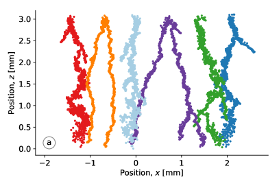
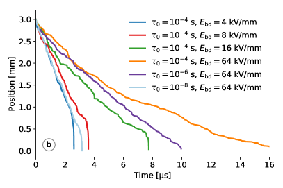
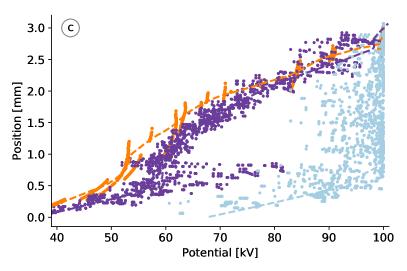
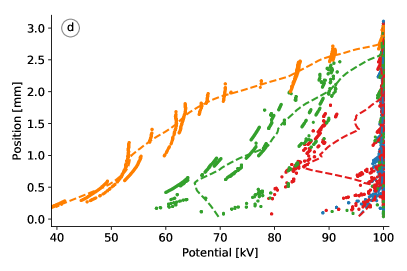
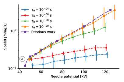
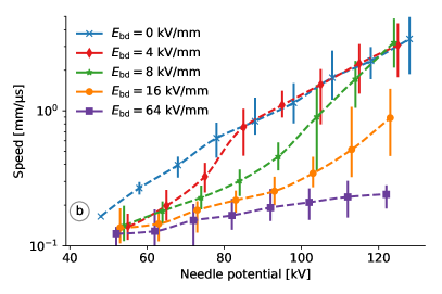
Figure 5: Simulations carried out at $100\text{\,}\mathrm{kV}$ using the same initial anion placement for a number of time constants $\tau_{0}$ and breakdown thresholds $E_{\textrm{bd}}$. (a) “Shadowgraphic plot” where the position of each streamer head is marked and (b) “streak plot” showing the leading streamer head vs time. (c) and (d) show the potential of streamer heads vs position, and can be compared with figure 4. They show how decreasing $\tau_{0}$ or $E_{\textrm{bd}}$, respectively, increases the average potential. Dots close to $100\text{\,}\mathrm{kV}$ in (d) indicate a recent channel breakdown (re-illumination). In (d), $E_{\textrm{bd}}=$4\text{\,}\mathrm{kV}\text{\,}{\mathrm{mm}}^{-1}$$ is close to maximum and mostly hidden behind the others. The dashed lines are moving averages. All streamer heads involved in each simulation is shown in (a), only the leading head is shown in (b). In (c) and (d), data is sampled every $3\text{\,}\mathrm{\SIUnitSymbolMicro m}$ of the propagation. Each dot in (b), (c) and (d) is also shown in (a), but not vice-versa.

Figure 6: Propagation speed calculated for the mid $1.5\text{\,}\mathrm{mm}$ of the gap. (a) for different time constants $\tau_{0}$ with $E_{\textrm{bd}}=$64\text{\,}\mathrm{kV}\text{\,}{\mathrm{mm}}^{-1}$$, and (b) for different breakdown thresholds $E_{\textrm{bd}}$ with $\tau_{0}=$e-4\text{\,}\mathrm{s}$$. Twenty simulations are performed for each voltage, the dashed lines are interpolated to the average values and the bars cover the minimum and maximum values. “Previous work” is data from [17] (figure 15, $E_{\alpha}=$2\text{\,}\mathrm{GV}\text{\,}{\mathrm{m}}^{-1}$$). Simulations where $\tau_{0}=$e-20\text{\,}\mathrm{s}$$ or $E_{\textrm{bd}}=$0\text{\,}\mathrm{kV}\text{\,}{\mathrm{mm}}^{-1}$$ are comparable to our previous work since $\tau$ is effectively zero for all of them. Each simulation is initiated with a random number to ensure that the configurations of seeds are uncorrelated.

For low channel conductivity, there is less “scatter” in the streamer potential, which makes it easier to interpret the results when investigating the effect of breakdown in the streamer channel, see figure 6(d). Breakdown in the channel can occur in the first part of the gap even when the threshold $E_{\textrm{bd}}$ is high, since a potential difference of some $\mathrm{kV}$ gives an electric field of several $\mathrm{kV}\text{\,}{\mathrm{mm}}^{-1}$ when the streamer length is some hundred $\mathrm{\SIUnitSymbolMicro m}$. For $E_{\textrm{bd}}=$16\text{\,}\mathrm{kV}\text{\,}{\mathrm{mm}}^{-1}$$ in figure 6(d), the average field inside the streamer is about $13\text{\,}\mathrm{kV}\text{\,}{\mathrm{mm}}^{-1}$. Rapid breakdowns gives $E_{\textrm{s}}$ close to zero for $E_{\textrm{bd}}=$8\text{\,}\mathrm{kV}\text{\,}{\mathrm{mm}}^{-1}$$, except for about $0.5\text{\,}\mathrm{mm}$ in the middle of the gap. The average field in a streamer is on the order of $\mathrm{kV}\text{\,}{\mathrm{mm}}^{-1}$ [20]. It is seen in figure 6(b) that the streamer slows down for the portion of the gap where the potential is decreased, and that streamers having similar average potential also use similar times to cross the gap.

Figure 6 gives a good qualitative indication of how $\tau_{0}$ and $E_{\textrm{bd}}$ affects the simulations. Different initial configuration of seed electrons show similar trends. Increasing concentration of seeds increases streamer propagation speed, but not branching [17]. However, changing the initial configuration changes the entire streamer breakdown and adds stochasticity to the model, while changing the needle voltage influences most results, such as the propagation speed, the jump distances, the number of branches, and the propagation length [17]. The effect of $\tau_{0}$ and $E_{\textrm{bd}}$ on the propagation speed is shown in figure 6 for a range of voltages, with several simulations performed at each voltage. The simulations with the lowest $\tau_{0}$ are similar to those with the lowest $E_{\textrm{bd}}$. For these simulations, the potential of the streamer is equal to the potential of the needle, and the results are similar to those presented in figure 15 in [17], as expected. Increasing $\tau_{0}$ can reduce the propagation speed for a given voltage, and the time constant seems to dampen the increase in speed following increased voltage. Adding the possibility of a breakdown in the channel reverses this, since the net effect is a reduction in the average time constant, i.e. an increase in net conductivity. At low needle potential, there are fewer breakdowns in the channel and the speed is mainly controlled by the conductivity through $\tau_{0}$, however, breakdowns become more frequent with increasing needle potential, which in turn increase the streamer potential and speed.

5 Discussion

As for our original model [17], this updated model still predicts a low propagation speed (see figure 6) and a low degree of branching (see figure 6(a)) compared with experimental results [29, 22]. Low propagation speed can be caused by low electron mobility, low electron/anion seed density, or too high shielding between streamer heads [17]. Increasing the time constant seems to increase the number of branches by regulating their speed and introducing breakdown in the channel reverses this effect. The hyperbole approximation of the electric field gives a strong electric field directed towards the planar electrode. Thus, electron avalanches in front of the head, giving forward propagation is favored over off-axis propagation and the chance of branching is reduced. A hyperbole can be a good approximation in the proximity of a streamer head, while possibly overestimating the potential in regions farther away. An overestimation of the potential from the streamer heads results in lower $k_{i}$ values for the heads, which in turn gives lower electric fields, slower streamers, and a higher probability of a branch stopping, especially for branches lagging behind the leading head. Since we model an “infinite” planar electrode, the capacitance does not change with the $xy$-position of an individual branch (unlike e.g. [14]). The coefficients $k_{i}$ scale the streamer heads when the electric potential from the streamer is calculated, and changing a $k_{i}$ can be interpreted as changing the capacitance of a streamer head. Two heads give a streamer a higher capacitance, but not twice the amount of a single head. However, the scaling is calculated from the potential and not the geometry, so this interpretation is an approximation, and for this reason we do not explicitly calculate the total capacitance or injected charge from the electrodes. The total injected current will reflect the behavior of individual heads discussed in section 3, having both a continuous component and impulses following breakdowns.

The conductivity of the channels can be approximated from the time constants. Consider that $d=$3\text{\,}\mathrm{mm}$$, $C=$0.1\text{\,}\mathrm{pF}$$, and $A=$100\text{\,}\mathrm{\SIUnitSymbolMicro}\mathrm{m}\mathrm{}\mathrm{2}$$, results in that $\sigma=$3\text{\,}\mathrm{S}\text{\,}{\mathrm{m}}^{-1}$$ is required for $\tau_{0}=$1\text{\,}\mathrm{\SIUnitSymbolMicro s}$$ according to 8. Figure 6 thus shows that a conductivity of some $\mathrm{S}\text{\,}{\mathrm{m}}^{-1}$ regulates the propagation speed, and that increased conductivity increases the speed. This is the order of magnitude as estimated for the streamer channel [2] and used by other models [14, 30], which is a very high conductivity compared with the liquid (about $e-13\text{\,}\mathrm{S}\text{\,}{\mathrm{m}}^{-1}$ [6]). A streamer propagating at $1\text{\,}\mathrm{km}\text{\,}{\mathrm{s}}^{-1}$ bridges a gap of $1\text{\,}\mathrm{mm}$ in $1\text{\,}\mathrm{\SIUnitSymbolMicro s}$, which implies that $\tau$ has to be shorter than this to have a significant effect on the propagation, in line with the results in figure 6. However, how frequent and how large the loss in potential is as the streamer propagates, is also important in this context.

The streamer model permits a streamer branch to propagate with a low reduction in potential, enabling a branch to propagate a short distance even when the channel is non-conducting. However, propagation and branching events increases the capacitance, which reduces the potential at the streamer head, and can result in a breakdown in the channel, i.e. a re-illumination. A re-illumination increases the potential of the streamer head, possibly causing other branches to be removed, and increases the chance of a new branching. A breakdown in the channel of one streamer head does not cause the nearby heads to increase in potential since each streamer head is individually “connected” to the needle (see figure 1). Streamer experiments sometimes show re-illumination of single branches [18], but often more than one branch light up at the same time, which is a limitation in the present model. Such effects can be investigated by further development towards an electric network model for the streamer channels and streamer heads [14].

A streamer channel is not constant in size, but grows and collapses dynamically [31]. This implies that $A$ in 4 changes with time, but so does $\sigma$, which depends on the density and mobility of the charge carriers. In turn, the creation, elimination, and mobility of the charge carriers is dependent on the pressure in the channel. Hence, it is not straightforward to evaluate how the conductivity of the channel is affected by the expansion. Conversely, external pressure reduces the diameter of the streamer channels [25], and reduce stopping lengths without affecting the propagation speed [32]. In a network model, each zigzag in each branch can be assigned specific parameters allowing greater control of the individual parts of the streamer, such as channel radius and conductivity. In the current implementation of the model, the channel length calculation and the constant conductivity (except for breakdowns), are aspects that can be improved in the future. Accounting for the actual length of the streamer channel is a minor correction, whereas branched streamer heads “sharing” parts of a channel can influence the simulation to a larger degree.

From section 3 we find that a channel with high conductivity has less frequent re-illuminations, in line with experiments [19]. The results in figure 4 and figure 6 also indicate that even with a collapsed channel (where low/none conductivity is assumed) a streamer is able to propagate some distance. Whereas experiments indicate that, 1st mode streamers may propagate only a short distance after the channel disconnects from the needle [33], but the stopping of second mode streamers occur prior to the channel collapsing [25]. In our model, restricting the conductivity reduces potential in the extremities of the streamer as the streamer propagates, which regulates the propagation speed and increases branching (figure 6). The potential is reduced until either the streamer stops, the propagation potential loss is balanced by conduction, or a re-illumination occurs and temporary increases the conductivity. This seems to contrast experimental results where the propagation speed of 2nd mode streamers is just weakly dependent on the needle potential [32] and re-illuminations does not change the speed [19]. However, whether a channel is “dark” or “bright” can affect the propagation speed of higher modes [34].

6 Conclusion

We have presented an RC-model which includes conductivity and capacitance of the streamer. This model has been applied in combination with a streamer propagation model based on the avalanche mechanism [17]. The RC-model introduces a time constant that regulates the speed of streamer propagation, depending on the conductivity of the channel and the capacitance in front of of the streamer. The streamer can propagate even when the channels are non-conducting, but then with reduction in potential which reduces the speed and may cause stopping. However, re-illuminations, breakdowns in the channel, increase its conductivity and the speed of the streamer. It is also found that streamer branching, which increases the capacitance and reduces the potential at the streamer heads, can give rise to re-illuminations. Some limitations of our previous model [17], such as the low propagation speed and low degree of branching, are not significantly affected by the addition of the RC-model, and need to be investigated further.

Appendix A Hyperbole capacitance

The electric field from a hyperbole is [17]

$$E=\frac{c}{a\sin\nu\sqrt{\sinh^{2}\mu+\sin^{2}\nu}}\,,$$ (14)

where $c$ and $a$ are constants given by the potential and the geometry, and $\mu$ and $\nu$ are prolate spheroid coordinates. In the $xy$-plane, $\sin\nu=1$ giving $\sinh^{2}\mu+1=\cosh^{2}\mu$, and $E$ becomes a function of the radius $r$,

$$E=\frac{c}{a\cosh\mu}=\frac{c}{\sqrt{r^{2}+a^{2}}}\,,$$ (15)

by using relations from [17]. The charge $Q$ of a system is given by the capacitance $C$ and the potential $V$ through $Q=CV$. The charge of the hyperbole is equal to the charge on the surface electrode, which is found by integration of the electric field using Gauss’ law

$$Q=2\pi\epsilon_{0}\int\limits_{0}^{R}E\,r\,\text{d}{r}=2\pi\epsilon_{0}c\left(\sqrt{R^{2}+a^{2}}-a\right)\,,$$ (16)

where $\epsilon_{0}$ is the vacuum permittivity. Implying that $Q\propto c$ for a plane of a finite radius $R\gg a$. From [35], $\left.c\approx{2V}\smash{\big{/}}{\ln(4a/r_{\textrm{p}})}\right.$ and by using $a=z+\frac{1}{2}r_{\textrm{p}}$, we find an expression for the capacitance of a hyperbole

$$C_{\textsc{h}}=\frac{Q}{V}\propto\frac{c}{V}=2\left({\ln\frac{4z+2r_{\textrm{p}}}{r_{\textrm{p}}}}\right)^{-1}\,,$$ (17)

which depends on the tip curvature $r_{\textrm{p}}$ and the distance from the plane $z$.

References

- [1] JC Devins, SJ Rzad, RJ Schwabe (1981) Breakdown and prebreakdown phenomena in liquids. J Appl Phys 52:4531–4545. doi:10/fnc58f
- [2] YV Torshin (1995) On the Existence of Leader Discharges in Mineral Oil. IEEE Trans Dielectr Electr Insul 2:167–179. doi:10/ffs58q
- [3] L Lundgaard, D Linhjell, G Berg, S Sigmond (1998) Propagation of positive and negative streamers in oil with and without pressboard interfaces. IEEE Trans Dielectr Electr Insul 5:388–395. doi:10/cn8k5w
- [4] JF Kolb, RP Joshi, S Xiao, KH Schoenbach (2008) Streamers in water and other dielectric liquids. J Phys D: Appl Phys 41:234007. doi:10/cxj7tm
- [5] RP Joshi, SM Thagard (2013) Streamer-like electrical discharges in water: Part I. fundamental mechanisms. Plasma Chem Plasma Process 33:1–15. doi:10/cxms
- [6] O Lesaint (2016) Prebreakdown phenomena in liquids: propagation ’modes’ and basic physical properties. J Phys D: Appl Phys 49:144001. doi:10/cxmf
- [7] P Wedin (2014) Electrical breakdown in dielectric liquids - a short overview. IEEE Electr Insul Mag 30:20–25. doi:10/cxmk
- [8] PJ Bruggeman, MJ Kushner, BR Locke, JGE Gardeniers, WG Graham, et al. (2016) Plasma–liquid interactions: a review and roadmap. Plasma Sources Sci Technol 25:053002. doi:10/cxmn
- [9] J Qian, RP Joshi, J Kolb, KH Schoenbach, J Dickens, et al. (2005) Microbubble-based model analysis of liquid breakdown initiation by a submicrosecond pulse. J Appl Phys 97:113304. doi:10/dmhk4f
- [10] J Jadidian, M Zahn, N Lavesson, O Widlund, K Borg (2014) Abrupt changes in streamer propagation velocity driven by electron velocity saturation and microscopic inhomogeneities. IEEE Trans Plasma Sci 42:1216–1223. doi:10/f55gj5
- [11] GV Naidis (2016) Modelling the dynamics of plasma in gaseous channels during streamer propagation in hydrocarbon liquids. J Phys D: Appl Phys 49:235208. doi:10/cxmg
- [12] L Niemeyer, L Pietronero, HJ Wiesmann (1984) Fractal dimension of dielectric breakdown. Phys Rev Lett 52:1033–1036. doi:10/d35qr4
- [13] AL Kupershtokh, DI Karpov (2006) Simulation of the development of branching streamer structures in dielectric liquids with pulsed conductivity of channels. Tech Phys Lett 32:406–409. doi:10/d3d7d3
- [14] I Fofana, A Beroual (1998) Predischarge Models in Dielectric Liquids. Jpn J Appl Phys 37:2540–2547. doi:10/bm4sd5
- [15] O Lesaint, G Massala (1998) Positive streamer propagation in large oil gaps: experimental characterization of propagation modes. IEEE Trans Dielectr Electr Insul 5:360–370. doi:10/dcvzh7
- [16] OL Hestad, T Grav, LE Lundgaard, S Ingebrigtsen, M Unge, O Hjortstam (2014) Numerical simulation of positive streamer propagation in cyclohexane. In 2014 IEEE 18th Int Conf Dielectr Liq, 1–5. doi:10/cxmd
- [17] I Madshaven, PO Åstrand, OL Hestad, S Ingebrigtsen, M Unge, O Hjortstam (2018) Simulation model for the propagation of second mode streamers in dielectric liquids using the Townsend-Meek criterion. J Phys Commun 2:105007. doi:10/cxjf
- [18] D Linhjell, L Lundgaard, G Berg (1994) Streamer propagation under impulse voltage in long point-plane oil gaps. IEEE Trans Dielectr Electr Insul 1:447–458. doi:10/chdqcz
- [19] NV Dung, HK Hoidalen, D Linhjell, LE Lundgaard, M Unge (2012) A study on positive streamer channels in Marcol Oil. In 2012 Annu Rep Conf Electr Insul Dielectr Phenom, 7491, 365–370. doi:10/czgj
- [20] A Saker, P Atten (1996) Properties of streamers in transformer oil. IEEE Trans Dielectr Electr Insul 3:784–791. doi:10/dgms5p
- [21] G Massala, O Lesaint (1998) Positive streamer propagation in large oil gaps: electrical properties of streamers. IEEE Trans Dielectr Electr Insul 5:371–380. doi:10/cfk7km
- [22] S Ingebrigtsen, HS Smalø, PO Åstrand, LE Lundgaard (2009) Effects of electron-attaching and electron-releasing additives on streamers in liquid cyclohexane. IEEE Trans Dielectr Electr Insul 16:1524–1535. doi:10/fptpt5
- [23] T Top, G Massala, O Lesaint (2002) Streamer propagation in mineral oil in semi-uniform geometry. IEEE Trans Dielectr Electr Insul 9:76–83. doi:10/dk4vtg
- [24] J Crowley (2008) Simple expressions for force and capacitance for a conductive sphere near a conductive wall. Proc Electrochem Soc Am Annu Meet Electrost Paper D1, pp 1–15. http://www.electrostatics.org/images/ESA_2008_D1.pdf
- [25] P Gournay, O Lesaint (1994) On the gaseous nature of positive filamentary streamers in hydrocarbon liquids. II: propagation, growth and collapse of gaseous filaments in pentane. J Phys D: Appl Phys 27:2117–2127. doi:10/dw59f5
- [26] GV Naidis (2015) On streamer inception in hydrocarbon liquids in point-plane gaps. IEEE Trans Dielectr Electr Insul 22:2428–2432. doi:10/gbf7x2
- [27] M Haidara, A Denat (1991) Electron multiplication in liquid cyclohexane and propane. IEEE Trans Electr Insul 26:592–597. doi:10/dk77wh
- [28] P Gournay, O Lesaint (1993) A study of the inception of positive streamers in cyclohexane and pentane. J Phys D: Appl Phys 26:1966–1974. doi:10/ck4hxg
- [29] S Ingebrigtsen, LE Lundgaard, PO Åstrand (2007) Effects of additives on prebreakdown phenomena in liquid cyclohexane: II. Streamer propagation. J Phys D: Appl Phys 40:5624–5634. doi:10/ck6k6q
- [30] T Aka-Ngnui, A Beroual (2006) Determination of the streamers characteristics propagating in liquids using the electrical network computation. IEEE Trans Dielectr Electr Insul 13:572–579. doi:10/b8dr5t
- [31] R Kattan, A Denat, O Lesaint (1989) Generation, growth, and collapse of vapor bubbles in hydrocarbon liquids under a high divergent electric field. J Appl Phys 66:4062–4066. doi:10/c9z5k2
- [32] O Lesaint, P Gournay (1994) On the gaseous nature of positive filamentary streamers in hydrocarbon liquids. I: Influence of the hydrostatic pressure on the propagation. J Phys D: Appl Phys 27:2111–2116. doi:10/d5q8x4
- [33] L Costeanu, O Lesaint (2002) On mechanisms involved in the propagation of subsonic positive streamers in cyclohexane. Proc 2002 IEEE 14th Int Conf Dielectr Liq ICDL 2002 143–146. doi:10/fhc926
- [34] W Lu, Q Liu (2016) Prebreakdown and breakdown mechanisms of an inhibited gas to liquid hydrocarbon transformer oil under positive lightning impulse voltage. IEEE Trans Dielectr Electr Insul 23:2450–2461. doi:10/f866wd
- [35] R Coelho, J Debeau (1971) Properties of the tip-plane configuration. J Phys D: Appl Phys 4:1266–1280. doi:10/fg43t7