Galactic resonance rings. Modelling of motions in the wide solar neighborhood

Abstract

Models of the Galaxy with analytical Ferrers bars can reproduce the residual velocities of OB-associations in the Sagittarius, Perseus and Local System stellar-gas complexes located within 3 kpc solar neighborhood. Ferrers ellipsoids with density distribution defined by power indices $n=1$ and 2 are considered. The success in the reproduction of the velocity in the Local System is due to the large velocity dispersion which weakens the resonance effects by producing smaller systematic motions. Model galaxies form nuclear, inner and outer resonance rings $R_{1}$ and $R_{2}$. The outer rings $R_{2}$ manage to catch twice more particles than the rings $R_{1}$. The outer Lindblad resonance of the bar (OLR) is located 0.4 kpc beyond the solar circle, $R_{OLR}=R_{0}+0.4$ kpc, corresponding to the bar angular velocity of $\Omega_{b}=50$ km s^-1 kpc^-1. The solar position angle with respect to the bar, $\theta_{b}$, providing the agreement between model and observed velocities is 40–52^∘. Unfortunately, models considered cannot reproduce the residual velocities in the Carina and Cygnus stellar-gas complexes. The redistribution of the specific angular momentum, $L$, is found near the Lindblad resonances of the bar (ILR and OLR): the average value of $L$ increases (decreases) at the radii a bit smaller (larger) than those of the resonances that can be connected with the existence of two types of periodic orbits elongated perpendicular to each other there.

1 Introduction

The presence of a bar in the Galaxy is the signpost of secular evolution of galaxy structure (Kormendy & Kennicutt, 2004). After the end of the epoch of violent galaxy-galaxy interactions ($\sim 7$ Gyr ago) secular processes causes the bar formation in disc galaxies. Observations suggest that the fraction of disc galaxies containing a bar decreases towards higher redshifts and that most massive galaxies form bars much earlier than lower mass ones (Sheth et al., 2008; Melvin, Masters et al., 2013). Modelling shows that time-scale over which a bar forms increases strongly with decreasing disc-to-total mass fraction (e.g. Athanassoula & Sellwood, 1986; Fujii et al., 2018). Though bars can spontaneously form in dynamically cold discs (Ostriker & Peebles, 1973), the bar fraction depends on the environment: in disk dominated galaxies tidal interactions can trigger bar formation (e.g. Elmegreen, Elmegreen & Bellin, 1990; Mendez-Abreu et al., 2012; Martinez-Valpuesta et al., 2017). The rigid rotation of the bar in the differentially rotating disc causes the appearance of the resonances and the formation of resonance rings (Buta, 2017).

There is a lot of evidence that our Galaxy includes a bar. Infrared observations of the inner Galactic plane (Dwek et al., 1995; Benjamin et al., 2005; Cabrera-Lavers et al., 2007; Churchwell et al., 2009; González-Fernández et al., 2012), gas kinematics in the inner Galaxy (Pohl et al., 2008; Gerhard, 2011), X-shaped distribution of red giants in the central region derived from BRAVA, WISE and VVV data (Li & Shen, 2012; Ness & Lang, 2016; Simion et al., 2017) confirm the presence of the bar in the Galaxy. The estimates of the length of the bar major semi-axis lie in the range 3–5 kpc which corresponds to the bar angular velocity 40–70 km s^-1.

The resonance between the frequency of orbital rotation with respect to the bar and the frequency of epicyclic motions causes the formation of the elliptical resonance rings (Buta, 1995; Buta & Combes, 1996). The condition of the resonance is following:

$$\frac{n}{m}=\frac{\kappa}{\Omega-\Omega_{b}},$$ (1)

where $n$ shows the number of full epicyclic revolutions which are made by a star rotating on a circular orbit around the galactic center during $m$ orbital revolution with respect to the bar. Usually the case of $m=1$ is considered. The fraction $n/m=\pm 2/1$ corresponds to the Inner Lindblad Resonance (ILR, $+2/1$) and the Outer Lindblad Resonance (OLR, $-2/1$) besides the high order resonances $\pm$4/1 are also important (Athanassoula, 1992; Contopoulos & Grosbol, 1989).

Modelling of the resonance rings shows that the outer rings are forming near the OLR of the bar while inner and nuclear rings are emerging near the inner 4/1 resonance and the ILR, respectively (Schwarz, 1981; Byrd et al., 1994; Rautiainen & Salo, 1999, 2000; Rodriguez-Fernandez & Combes, 2008; Pettitt et al., 2014; Li, Shen & Kim, 2015; Sormani et al., 2018).

The outer rings have two preferable orientations with respect to the bar: the rings $R_{1}$ are elongated perpendicular to the bar while the rings $R_{2}$ are stretched along the bar. Of two outer rings, $R_{1}$ lies a bit closer to the galactic center than $R_{2}$. Some of them don’t have pure elliptical shape but include a break so that they rather resemble two tightly wound spiral arms. Broken rings are named pseudorings and are marked with apostrophe, for example, $R_{1}^{\prime}$ and $R_{2}^{\prime}$ (Buta, 1995; Buta & Combes, 1996; Buta & Crocker, 1991).

All resonance rings are supported by main periodic orbits. The main periodic orbits are stable orbits close to the circular ones in the unperturbed case. Such orbits are followed by a large set of quasi-periodic orbits. There are two basic families of stable direct periodic orbits, $x_{1}$ and $x_{2}$. The family $x_{2}$ of stable periodic orbits exists only between two ILRs. There is also a third family of periodic orbits, $x_{3}$, which consists of unstable orbits. The main periodic orbits $x_{1}$ inside the corotation radius (CR) are elongated along the bar and form the backbone of the bar. The $x_{2}$ orbits are elongated perpendicular to the bar and support the nuclear rings. Near the OLR of the bar the main family of periodic orbits $x_{1}$ is splitting into two families: $x_{1}(1)$ and $x_{1}(2)$. The main stable periodic orbits $x_{1}(2)$ lying between the $-4/1$ and $-2/1$ (OLR) resonances are elongated perpendicular to the bar while orbits $x_{1}(1)$ located outside the OLR are stretched along the bar. Periodic orbits $x_{1}(2)$ support outer rings $R_{1}$ while orbits $x_{1}(1)$ support outer rings $R_{2}$. (Contopoulos & Papayannopoulos, 1980; Contopoulos & Grosbol, 1989; Schwarz, 1981; Buta & Combes, 1996).

Study of invariant manifolds associated with unstable periodic orbits around Lagrangian equilibrium points $L_{1}$ and $L_{2}$ shows that they can also give rise to spiral-like and ring-like structures in barred galaxies (Romero-Gómez et al., 2007; Athanassoula et al., 2009; Jung & Zotos, 2016).

Analysis of the mid-infrared images of galaxies detected by the Spitzer Space Telescope (Sheth et al., 2010) reveals that the fraction of galaxies hosting outer rings or preudorings increases with increasing bar strength from 15 (SA) to 32 per cent (SAB) and then drops to 20 per cent for stronger bars (SB) (Comeron et al., 2014).

Elmegreen & Elmegreen (1985) discover two types of bars: large bars with nearly a constant surface brightness mostly found in early type galaxies and smaller bars with nearly exponential profiles mainly observed in late-type galaxies. Laurikainen, Salo & Buta (2005) show that ”flat” bars in early-type galaxies can be described well either by a Sérsic or a Ferrers function.

The presence of the outer rings in the Galaxy was first suggested by Kalnajs (1991). The main advantage of models with outer rings is that they don’t need spiral-like potential perturbation to create long-lived elliptical structures at the galactic periphery. Outer rings are forming in 200-500 Myr after the bar formation and can exist for several Gyrs (Rautiainen & Salo, 2000; Rautiainen & Melnik, 2010).

The angle between the major axis of the bar and the Sun–Galactic center line or the so-called solar position angle with respect to the bar, $\theta_{b}$, derived from data of the infrared surveys (GLIMPSE, 2MASS, and VVV) has the value of 40–45^∘ so that the end of the bar closest to the Sun is located in the first quadrant (Benjamin et al., 2005; Cabrera-Lavers et al., 2007; González-Fernández et al., 2012). Besides, a reconstruction of the Galactic CO maps with smoothed particle hydrodynamics gives the best results for the solar position angle of $\theta_{b}\approx 45^{\circ}$ (Pettitt et al., 2014).

Melnik & Rautiainen (2009) using models with analytical Ferrers bars study the Galactic kinematics in the 3 kpc solar neighborhood. Their models form the two-component outer rings $R_{1}R_{2}^{\prime}$ after $\sim 800$ Myr from the start of simulation. The gas subsystem includes 5 10⁴ massless gas particles which can collide with each other inelastically. The best agreement between model and observed velocities corresponds to the solar position angle $\theta_{b}=45\pm 5^{\circ}$. These models can reproduce the average velocities of OB-associations in the Perseus and Sagittarius stellar-gas complexes but failed in the Local System, Cygnus and Carina stellar-gas complexes.

The fact that the position angle of the Sun with respect to the bar, $\theta_{b}$, is close to 45^∘ means that the 3-kpc solar neighbor can harbor both a segment of the outer ring $R_{1}$ and a segment of the ring $R_{2}$. The study of the distribution of classical Cepheids and young open clusters reveals the existence of ”the tuning-fork-like” structure which can be interpreted as two segments of the outer rings fusing together near the Carina stellar-gas complex (Melnik et al., 2015, 2016). Note also that models with the two-component outer ring $R_{1}R_{2}^{\prime}$ can explain the position of the Sagittarius-Carina arm in the Galactic disc: a segment of the ring $R_{1}$ outlines the Sagittarius arm while an arch of the outer ring $R_{2}$ lies in the vicinity of the Carina arm (Melnik & Rautiainen, 2011).

Rautiainen & Melnik (2010) build N-body models of the Galaxy which demonstrate the development of a bar and the formation of the outer rings which being formed persist till the end of simulation (6 Gyr). The special feature of N-body models is fast changes of velocities of model particles which can be separated into quick stochastic changes due to irregular forces and quasi-periodic slow oscillations due to slow modes (patterns rotating slower than the bar). Thus, the averaging of model velocities over a large time interval is required for a comparison with observed velocities. In N-body models by Rautiainen & Melnik (2010), the velocities of model particles are averaged over the time interval of 1 Gyr in the reference system corotating with the bar. The averaged model velocities appear to be able to reproduce the observed velocities in the Sagittarius, Perseus and Local System stellar-gas complexes. The advantage of models without self-gravity in kinematical studies is that they enable us to compare observe and model velocities directly without averaging.

Models presented here don’t include spiral arms because both resonance rings and spiral arms are invoking to explain the same things: the systematic velocity deviations from the rotation curve and the increased density of young objects in some regions. Any travelling spiral density wave (Lin & Shu, 1964) winds up around the Lindblad resonances after a few time revolution periods (Toomre, 1969). The mechanism (WASER) including the reflection of the travelling wave in the central region can support a steady spiral pattern (Mark, 1976; Bertin & Lin, 1996) but it gives small amplification to support the shock fronts as well (Athanassoula, 1984; Binney & Tremaine, 1987). The shock fronts forming in spiral arms due to collisions in gas subsystem act in the same direction causing the drift of gas from the CR towards the Lindblad resonances (Toomre, 1977). Another conception of the galactic spiral structure suggests short transient spiral arms forming in self-gravitating galactic discs due to swing amplification mechanism (Julian & Toomre, 1966; Toomre, 1981). This mechanism can be very powerful and transient ragged spiral arms often appear in simulations with live discs (Pettitt et al., 2015; Baba et al., 2009, 2013; Grand et al., 2012; D’Onghia et al., 2013, and other papers). However, the pitch angle of these short-lived arms is quite large, $i=20\textrm{--}30^{\circ}$. The theoretical prediction of its value is $i=24^{\circ}$ (Melnik & Rautiainen, 2013; Michikoshi & Kokubo, 2014). But the Galactic global spiral arms seem to have a considerably smaller pitch angle, $10\textrm{--}15^{\circ}$ (for example, Georgelin & Georgelin, 1976; Russeil, 2003; Vallée, 2015, and references therein). Generally, the conception of the Galactic spiral arms has a lot of difficulties. Nevertheless, many kinematical and morphological features of the Galaxy can be explained in terms of spiral arms (Rastorguev et al., 2017; Bobylev & Bajkova, 2018; Xu et al., 2018; Grosbøl & Carraro, 2018; Antoja et al., 2018; Kawata et al., 2018; Ramos, Antoja & Figueras, 2018, and other papers).

In this paper I present several models with analytical Ferrers bars which can reproduce the observed velocities in the Sagittarius, Perseus and Local System stellar-gas complexes. The crucial factor which determines the success in the Local System appears to be a large velocity dispersion which weakens the resonance effects. Section 2 considers the distribution of observed velocities of young stars in the Galactic disc; Section 3 describes the models; Section 4 compares model and observed velocities, studies the distribution of the surface density, velocity dispersions and the angular momentum along the radius; Section 5 infers the main conclusions.

2 The observed velocities of OB-associations in the 3-kpc solar neighborhood

The velocities of OB-associations give the most reliable information about the distribution of velocities of young objects in a wide solar neighborhood. The catalog by Blaha & Humphreys (1989) includes 91 OB-associations, $\sim 85$ per cent of which include at least one star of spectral types earlier than B0, whose age is supposed to be less than 10 Myr (Bressan et al., 2012), so the average velocities of OB-associations must be very close to the velocities of their parent giant molecular clouds. Here we consider velocities obtained with Gaia DR2 proper motions (Brown et al., 2018; Lindegren et al., 2018; Katz et al., 2018). Note that the sky-on velocities of OB-associations derived from Gaia DR1 and from Gaia DR2 proper motions differ on average by 2 km s^-1 (for more details see Melnik & Dambis, 2017, 2018).

For comparison with models we use the residual velocities of OB-associations which characterize non-circular motions in the Galactic disc. The residual velocities are determined as differences between the observed heliocentric velocities and the velocities due to the Galactic circular rotation curve and the solar motion towards the apex ($V_{res}=V_{obs}-V_{rot}-V_{ap}$). The radial and azimuthal components, $V_{R}$ and $V_{T}$, of the residual velocity are positive if they are directed away from the Galactic center and in the sense of Galactic rotation, respectively. The residual velocity along z-axis, $V_{z}$, is positive in the direction toward the North Galactic pole. The parameters of the rotation curve and solar motion are derived from the entire sample of OB-associations with known line-of-sight velocities and Gaia DR2 proper motions (Melnik & Dambis, 2017, 2018). Residual velocities determined with respect to a self-consistent rotation curve are practically independent of the choice of the value of $R_{0}$.

Figure 1 shows the residual velocities of OB-associations in the Galactic plane. To mitigate the random errors, we average the residual velocities of OB-associations within the volumes of the stellar-gas complexes identified by Efremov & Sitnik (1988). Table 1 gives the name of the stellar-gas complex, its Galactocentric distance $R$, the list of OB-associations related to it, the range of their Galactic longitudes $l$ and heliocentric distances $r$, their average residual velocities: $V_{R}$, $V_{T}$ and $V_{z}$. The OB-associations having at leat 2 stars with known line-of-sight velocities and Gaia DR2 proper motions are considered.

The Galactocentric distance of the Sun is adopted to be $R_{0}=7.5$ kpc (Glushkova et al., 1998; Nikiforov, 2004; Feast et al., 2008; Groenewegen, Udalski & Bono, 2008; Reid et al., 2009; Dambis et al., 2013; Francis & Anderson, 2014; Boehle et al., 2016; Branham, 2017). The choice of $R_{0}$ in the range 7–9 kpc has small influence on the residual velocities.

Figure 1 and Table 1 indicate that the majority of OB-associations in the Perseus complex have the radial component of the residual velocity, $V_{R}$, directed toward the Galactic center while the velocities $V_{R}$ of most of OB-associations in the Sagittarius and Local System complexes are directed away from the Galactic center. As for the azimuthal residual velocities, the majority of OB-associations in the Perseus complex have $V_{T}$ directed in the sense opposite that of Galactic rotation while $V_{T}$ is close to zero in the Sagittarius and Local System complexes. It is just the residual velocities in the Sagittarius, Perseus and Local System stellar-gas complexes that can be reproduced in present dynamical models.

However, the residual velocities in the Cygnus and Carina complexes are still remaining a stumbling block for numerical simulations. That concerns both types of models: those with analytical bars and N-body simulations (Melnik & Rautiainen, 2009; Rautiainen & Melnik, 2010).

Table 1 also shows that the average velocities in the z-direction, $V_{z}$, are close to zero. Here we suppose that motions in the Galactic plane and in the z-direction are independent that allows us to use 2D models.

Note that models considered must also reproduce the Galactic rotation curve determined for the sample of OB-associations. To avoid the systematical effects, we must use the same sample of objects for a study of residual velocities and for a determination of the parameters of rotation curve. The rotation curve derived from the velocities of OB-associations is nearly flat and corresponds to the angular velocity at the solar distance of $\Omega_{0}=31\pm 1$ km s^-1 kpc^-1 (Melnik & Dambis, 2017, 2018).

Table 1: The observed residual velocities of OB-associations in the stellar-gas complexes with Gaia DR2 data

Complex	R	$V_{R}$	$V_{T}$	$V_{z}$	l	r	Associations
	kpc	km s-1	km s-1	km s-1	deg.	kpc
Sagittarius	6.0	$+7.5\pm 2.1$	$-0.3\pm 1.7$	$-0.6\pm 1.8$	8–23∘	1.3–1.9	Sgr OB1, OB4, OB7, Ser OB1, OB2, Sct OB3;
Carina	6.9	$-6.2\pm 2.6$	$+6.2\pm 2.8$	$-1.9\pm 0.7$	286–315∘	1.5–2.1	Car OB1, OB2, Cru OB1, Cen OB1,
							Coll 228, Tr 16, Hogg 16, NGC 3766, 5606;
Cygnus	7.3	$-4.3\pm 1.3$	$-10.3\pm 1.4$	$+2.0\pm 1.4$	73–78∘	1.0–1.8	Cyg OB1, OB3, OB8, OB9;
Local System	7.8	$+5.4\pm 2.6$	$+1.2\pm 2.6$	$-0.1\pm 0.5$	0–360∘	0.3–0.6	Per OB2, Ori OB1, Mon OB1, Vela OB2,
							Coll 121, 140;
Perseus	8.8	$-4.7\pm 2.2$	$-4.4\pm 1.7$	$+0.5\pm 0.6$	104–135∘	1.8–2.8	Cep OB1, Per OB1, Cas OB1, OB2, OB4,
							OB5, OB6, OB7, OB8, NGC 457;

Figure 1: Distribution of the residual velocities of OB-associations in the Galactic plane. The residual velocities are derived with the use of Gaia DR2 proper motions. OB-associations with residual velocities $|V_{R}|$ and $|V_{T}|$ smaller than 3 km s^-1 are shown as the black circles without any vector. The ellipses indicate the positions of the Sagittarius, Carina, Cygnus, Local System (LS), and Perseus stellar-gas complexes. The x- and y- axes are directed towards the Galactic rotation and away from the Galactic center, respectively. The Sun is at the origin.

3 Models

I have built several models with analytical Ferrers bars (Ferrers, 1877) which can reproduce the kinematics in the Perseus, Sagittarius, and Local System stellar-gas complexes. Some of them are discussed here.

Table 2 lists the general parameters of model 1: the time of simulation $T$, the time step of integration $\Delta t$, the number of particles $N$. We neglect the self-gravity between model particles. The massless test particles can be thought as low-mass gas clouds moving in the potential created by the stellar subsystem. The orbits of model particles are calculated with the use of leapfrog method.

All models include a bar, a disc, a bulge and halo, whose parameters are given in Table 2. The bar is modelled as a Ferrers ellipsoid with volume-density distribution $\rho$ defined as follows:

$$\rho=\left\{\begin{array}[]{l}\rho_{0}(1-\mu^{2})^{n},\ \mu\leq 1\\ \\ 0,\ \mu>1,\\ \end{array}\right.$$ (2)

where $\mu$ equals $\mu^{2}=x^{2}/a^{2}+(y^{2}+z^{2})/b^{2}$ but $a$ and $b$ are the lengths of the major and minor semi-axes of the bar, respectively. Here we consider 2D-models, so $z=0$. The acceleration created by the bar depends on the mass of the bar $M_{b}$, semi-axes $a$ and $b$, the coordinates ($x$, $y$) reckoned with respect to the bar axes and the power index $n$ (de Vaucouleurs & Freeman, 1972; Pfenniger, 1984; Binney & Tremaine, 1987; Sellwood & Wilkinson, 1993).

The angular velocity of the bar, $\Omega_{b}$, providing the best agrement with observations appears to be $\Omega_{b}=50$ km s^-1 kpc^-1. The non-axisymmetric perturbations of the bar grows slowly approaching the full strength during $T_{gr}=492$ Myr equal to four bar revolution periods. However, $m=0$ component of the bar is included in models from the beginning. It can be interpreted as a pre-existent disc-like bulge (Athanassoula, 2005). The mass of the bar, $M_{b}=1.30\times 10^{10}$M_⊙, agrees with other estimates (e.g. Dwek et al., 1995).

Models include an exponential disc with the scale length $R_{d}$:

$$\Sigma=\Sigma_{0}\;e^{-R/R_{d}},$$ (3)

where $\Sigma$ and $\Sigma_{0}$ are the surface densities at the radius $R$ and at the galactic center, respectively. The velocity of the rotation curve, $V_{c}$, produced by exponential disc is determined by the following relation:

$$V_{c}^{2}=4\pi G\Sigma_{0}R_{d}y^{2}[I_{0}(y)K_{0}(y)-I_{1}(y)K_{1}(y)],$$ (4)

where $y=0.5R/R_{d}$ while $I_{n}$ and $K_{n}$ are modified Bessel functions of order $n$ of the first and second kinds, respectively (Freeman, 1970; Binney & Tremaine, 1987).

Here the mass of the disc is adopted to be $M_{d}=3.5\times 10^{10}$M_⊙. To compare with a disc mass in N-body simulations we should sum the mass of the disc and some part of that of the bar. The total value, $3.5\textrm{--}4.8\times 10^{10}$M_⊙, is consistent with other estimates of the Galactic disc mass, 3.5–5.0$\times 10^{10}$M_⊙ (Shen et al., 2010; Fujii et al., 2019).

The classical bulge determines the potential in the galactic center, it is modelled by a Plummer sphere (for example, Binney & Tremaine, 1987) whose rotation curve is defined by following expression:

$$V_{c}^{2}(R)=\frac{GM_{bg}{R}^{2}}{(R^{2}+R_{bg}^{2})^{3/2}},$$ (5)

where $M_{bg}$ and $R_{bg}$ are the mass and characteristic length of the bulge. The mass of the Galactic classical bulge is expected to lie in the range 3–6 $\times 10^{9}$M_⊙ and the adopted value is $M_{bg}=5\times 10^{10}$ here (e.g., Dehnen & Binney, 1998; Nataf, 2017; Fujii et al., 2019).

The halo dominates on the galactic periphery. It is modelled as an isothermal sphere with following rotation curve:

$$V_{c}^{2}(r)=V_{max}^{2}\frac{R^{2}}{R^{2}+R_{h}^{2}},$$ (6)

where $V_{max}$ is the asymptotic maximum on the halo rotation curve and $R_{h}$ is the core radius.

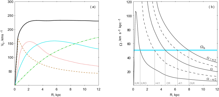
Figure 2: (a) Model rotation curves. The thick black line shows the total rotation curve while the dashed, dotted, solid and dash-dotted lines (colored brown, red, blue, green in electronic edition) indicate the contribution of the bulge, bar, disc and halo, respectively. (b) Dependence of the angular velocities on the galactocentric distance $R$. The continuous curves represent the angular velocities $\Omega$ and $\Omega\pm\kappa/2$ while the dashed lines indicate $\Omega\pm\kappa/4$. The horizontal thick line (colored blue in electronic edition) shows the angular velocity of the bar, $\Omega_{b}=50$ km s^-1 kpc^-1. The resonance distances are determined by its intersections with the curves of angular velocities.

Figure 2(a) shows the total rotation curve produced by the gravitation of the bulge, bar, disc and halo. The total rotation curve is nearly flat with the average azimuthal velocity of $\Theta=232$ km s^-1. This model value corresponds to the angular velocity at the solar distance ($R_{0}=7.5$ kpc) of $\Omega_{0}=30.9$ km s^-1 kpc^-1 and is consistent with observations, $\Omega_{0}=31\pm 1$ km s^-1 kpc^-1(Melnik & Dambis, 2017, 2018). Model and observed rotation curves are in good agreement with each other, at least in the 3-kpc solar neighborhood.

Figure 2(b) demonstrates the positions of the resonances which correspond to the intersections of the horizontal line indicating the angular velocity of the bar ($\Omega_{b}=50$ km s^-1kpc^-1) with the appropriate curves of angular velocities. Note that present models include two inner Lindblad resonances (ILRs): outer (ILRO) and inner (ILRI) ones. The CR of the bar lies at the radius of 4.6 kpc near the end of the Ferrers ellipsoid ($a=4.2$ kpc), so the model bar is dynamically fast (Debattista & Sellwood, 2000; Rautiainen et al., 2008).

The models can be rescaled for a bit different values of the solar Galactocentric distance $R_{0}$. It is possible due to the fact that the Galactic rotation curve is flat in the solar neighborhood. If the ratio of the new and old values of $R_{0}$ is $q=(R_{new}/R_{old})$ then the masses of the bulge, bar and disk must be changed by a factor of $\sim q^{2}$ but the asymptotic velocity of the halo – by a factor of $\sim q$. New rotation curve will be also flat in the solar neighborhood.

If test particles approach each other at a small distance, $\varepsilon$, they can collide with each other inelastically imitating the behavior of a gas subsystem (Brahic & Henon, 1977; Levinson & Roberts, 1981; Roberts & Hausman, 1984). Collisions are adopted to be absolutely inelastic, so the velocities of two gas particles after a collision are the same $\bf v_{1}^{\prime}=v_{2}^{\prime}$ equal to $({\bf v_{1}}+{\bf v_{2}})/2$, where $\bf v$ and $\bf v^{\prime}$ are the velocities before and after a collision, respectively.

The changes of velocities due to collisions at each step are performed before the leapfrog integration. To accelerate the computation of collisions we sort particles in the ascending order of the coordinate $x$ at each step of integration as it is supposed by Salo (1991).

There is a danger that a pair of gas particles can fall into ”permanent collisions” (Brahic & Henon, 1977), i. e. the same two particles would collide at each step of integration. The galactic differential rotation can tear some close pairs of colliding particles but it is powerless for particles lying at the same galactic radius. The main remedy against ”permanent collisions” is quite large velocity dispersion in radial direction maintained above some minimal level, $\sigma_{min}$, throughout the galactic disc. ”Permanent collisions” can be avoided if the average distance passed by a particle relative to another during one step of integration $\Delta t$ is always larger than the length of collision, $\varepsilon$:

$$\sqrt{2}\;\sigma_{min}\>\Delta t\geq\varepsilon.$$ (7)

Epicyclic motions and perturbations from the bar increase the velocity dispersion while collisions decrease it. The parameter $\varepsilon$ regulates the frequency of collisions which grows with increasing $\varepsilon$. The choice of the initial velocity dispersion $\sigma_{0}$ equal to 5 km s^-1 and $\varepsilon$ of 0.05 pc (Table 2) provides the velocity dispersion, $\sigma_{R}$, never dropping below 5 km s^-1, so the condition (7) is always fulfilled (see also section 4.4).

Two colliding gas particles have a probability, $P_{c}$, that one of them forms an OB-association which wouldn’t take part in collisions during some time interval, $t_{ob}$. OB-particles move ballistically but after time $t_{ob}$ they transform back into gas particles resuming their ability to collide (Roberts & Hausman, 1984; Salo, 1991). The interest to OB-particles is due to the fact that they indicate the places with the highest density of model particles and outline the positions of different morphological structures. Generally, OB-particles only roughly imitate the process of the formation of OB-associations. Values of $P_{ob}$ and $t_{ob}$ are usually taken to be 10 per cent and 4 Myr, respectively (Table 2).

The initial surface density of model particles in model 1 is uniform within the radius $R<11$ kpc (Table 2).

Model 1 is a basic model of our study. But we also consider three other models which differ from model 1 in one of the following features: the initial distribution, presence/absence of collisions and the power index $n$ of the density distribution inside the Ferrers ellipsoid. Model 2 starts from an exponential distribution of gas particles in the galactic plane with the scale length of $r_{d}=2.5$ kpc but values of all other parameters coincide with those of model 1. Model 3 is collisionless and that is its only difference from model 1. Model 4 includes the Ferrers bar whose density distribution is determined by the power index $n=1$, i. e. its bar is less centrally concentrated than in other models, but the mass of the bar, $M_{b}$, and all other parameters are the same as in model 1. Table 3 briefly characterizes models 1–4 and presents the total number of collisions, $N_{c}$, occurred during the simulation time.

All models considered have the same angular velocity of the bar, $\Omega_{b}=50$ km s^-1 kpc^-1. As the distribution of the potential is the same in Models 1–3, the locations of the resonances must also be the same there. Formally, model 4 differs from models 1–3 in the potential distribution but that weakly affects the positions of the resonances. Table 4 presents the resonance locations in models 1–3 and in model 4. It is seen that the difference in the resonance radii doesn’t exceed 0.1 kpc and mainly concerns the ILRO and +4/1 resonance, but the radius of the OLR is the same in all models considered.

The amount of non-axisymmetric perturbations produced by the bar is usually estimated through the parameter $Q_{T}(R)$, which is the ratio of the maximal tangential force at some radius to the azimuthally average radial force at the same radius:

$$Q_{T}(R)=\frac{\max(|F_{T}|)}{<|F_{R}|>}.$$ (8)

The value of $Q_{T}$ varies with radius. Its maximal value is named $Q_{b}$ and is usually used as a measure of the strength of the bar:

$$Q_{b}=\max[Q_{T}(R)]$$ (9)

(Sanders & Tubbs, 1980; Combes & Sanders, 1981; Athanassoula et al., 1983).

Figure 3 shows the variations of $Q_{T}$ along the galactic radius calculated for models 1–3 and for model 4. Maximal values of $Q_{T}$ are 0.380 (models 1–3) and 0.367 (model 4). They are achieved at the distances of 1.8 and 2.2 kpc, respectively. The value of the bar strength $Q_{b}\approx 0.38$ is quite expectable for galaxies with strong bars (Block et al., 2001; Buta, Laurikainen & Salo, 2004; Díaz-García et al., 2016). Note that at the distance of the OLR, $R=7.9$ kpc, the value of $Q_{T}$ is larger in model 4 ($Q_{T}=0.0074$) than in models 1–3 ($Q_{T}=0.0057$) by  25 per cent. This small preponderance of model 4 being amplified by the resonance results in larger velocity perturbations produced by model 4 in the solar neighborhood.

The value of the bar strength, $Q_{b}$, is sensitive to the choice of the bulge mass: the larger $M_{bg}$ the smaller $Q_{T}$. For example, the increase of $M_{bg}$ from 5 to $9\times 10^{9}$M_⊙ results in the decrease of $Q_{b}$ from 0.38 to 0.34.

Figure 4 shows the distribution of model particles at three time moments: 0.5, 1.0 and 1.5 Gyr. The frames related to models 1, 2 and 4 demonstrate the distribution of OB-particles. Model 3 is collisionless, so OB-particles aren’t forming there, the corresponding frames merely present the distribution of 10 per cent of model particles. We can see that model discs form nuclear rings ($\sim 0.5$ kpc) and conspicuous outer rings $R_{2}$ ($\sim 9.0$ kpc). Model galaxies also produce outer rings $R_{1}$ ($\sim 6$ kpc) and inner rings ($\sim 3$ kpc) which are mainly noticeable in the density profiles (section 4.3). Note that all models demonstrate the diamond-shape structures which are located inside the Ferrers ellipsoids and indicate the places of most densely populated bar orbits. These structures aren’t inner rings which usually have more round shapes and are forming outside the bar. Model 2 ($t=0.5$ Gyr) gives a good example of an inner ring which touches the bar only at the bar ends. Models 1 and 3 also include inner rings but they are hardly visible in Figure 4 (see section 4.3). The nuclear and inner rings are forming quickly and are already existent at the time $t=0.5$ Gyr when the bar acquires its full strength. The outer rings are growing slower: they appear as pseudorings at $t=0.5$ Gyr and take pure elliptical shape at the time $t\approx 1.0$ Gyr. Once formed, the outer rings exist to the end of simulation.

Table 2: General parameters of model 1

Simulation time	$T=2$ Gyr
Step of integration	$\Delta t=0.01$ Myr
Number of particles	$N=10^{5}$
Bulge	$R_{bg}=0.30$ kpc
	$M_{bg}=5$ 109M⊙
Bar	$a=4.2$ and $b=1.35$ kpc
	$M_{b}=1.30$ 1010M⊙
	$\Omega_{b}=50.0$ km s-1 kpc-1
	$T_{gr}=492$ Myr
Disc	exponential, $R_{d}=2.5$
	$M_{d}=3.5$ 1010M⊙
Halo	$R_{h}=8$ kpc
	$V_{max}=206$ km s-1
Collisions	absolutely inelastic
	$\varepsilon=0.05$ pc
OB-particles	$t_{ob}=4$ Myr – lifetime
	$P_{c}=0.1$ – probability
Initial distribution	uniform within $R<11$ kpc
	$\sigma_{0}=5$ km s-1

Table 3: Characteristics of models 1–4

Model	Initial distribution	$n$	$N_{c}$
1	uniform within $R<11$ kpc	$n=2$	3.6 107
2	exponential, $r_{d}=2.5$ kpc	$n=2$	4.7 107
3	uniform within $R<11$ kpc	$n=2$	0
4	uniform within $R<11$ kpc	$n=1$	3.6 107

Table 4: Locations of the resonances

Name	Definition	Models 1–3	Model 4
		$R$, kpc	$R$, kpc
OLR	$\kappa/(\Omega-\Omega_{b})=-2/1$	7.91	7.91
-4/1	$\kappa/(\Omega-\Omega_{b})=-4/1$	6.29	6.29
CR	$\Omega=\Omega_{b}$	4.61	4.62
+4/1	$\kappa/(\Omega-\Omega_{b})=4/1$	3.01	2.92
ILRO	$\kappa/(\Omega-\Omega_{b})=2/1$	0.97	0.92
ILRI	$\kappa/(\Omega-\Omega_{b})=2/1$	0.13	0.13

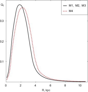
Figure 3: Variations of the parameter $Q_{T}$ along the galactic radius, $R$, in models 1–3 and in model 4. The power index $n$ equals $n=2$ and $n=1$ in models 1–3 and in model 4, respectively, while other parameters determined the potential are the same. Maximal value of $Q_{T}$ amounts to 0.380 in models 1–3 and to 0.367 in model 4. However, at the distance of the OLR, 7.9 kpc, the value of $Q_{T}$ is larger in model 4 ($Q_{T}=0.0074$) than in models 1–3 ($Q_{T}=0.0057$).

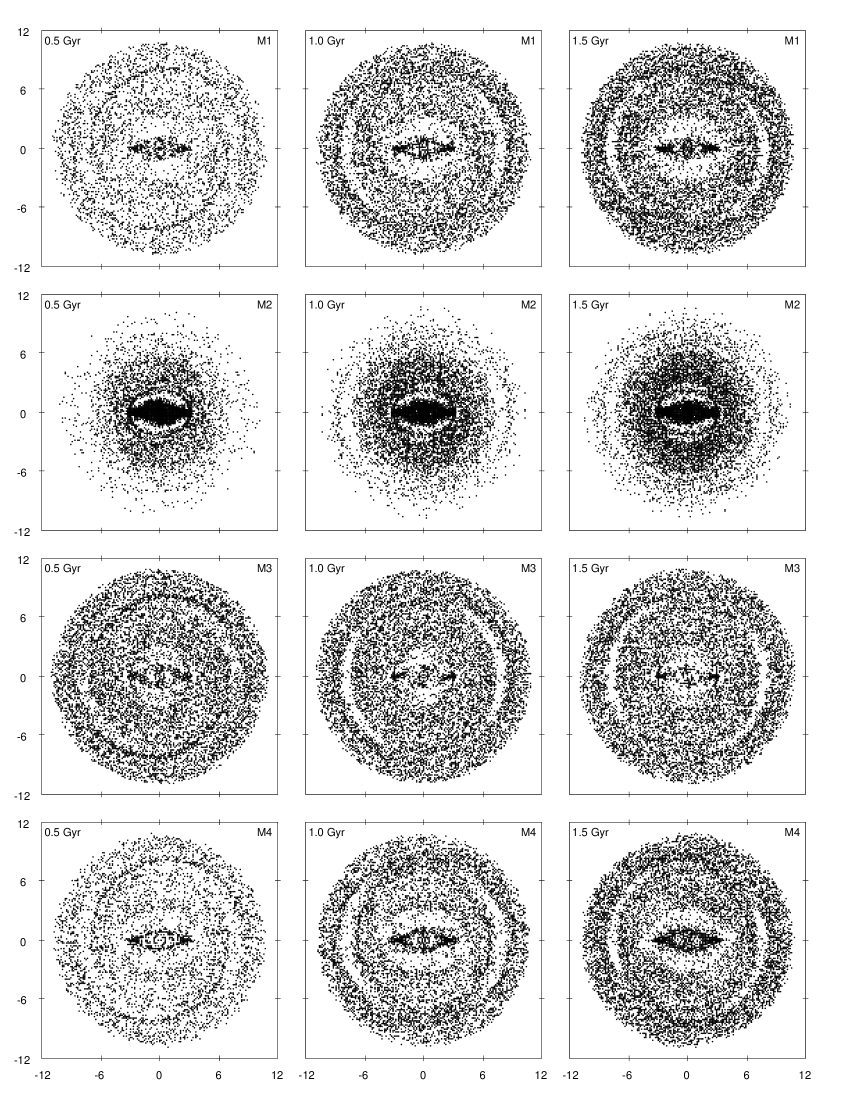
Figure 4: Distribution of model particles at three time moments: 0.5, 1.0 and 1.5 Gyr. Frames related to models 1, 2 and 4 display the distribution of OB-particles while model 3 demonstrates the distribution of 10 per cent of collisionless particles. The size of frames is $24\times 24$ kpc.

4 Results

4.1 Kinematics of model particles in the solar neighborhood

The epicyclic motions of model particles located near the OLR of the bar are adjusted in accordance with the perturbations coming from the bar that results in the formation of conspicuous systematic velocities.

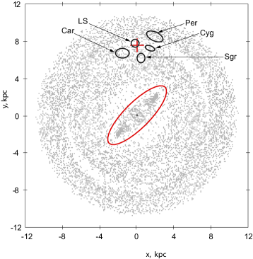
Figure 5: Distribution of OB particles (gray points) in the galactic plane. Also shown are the boundaries of the stellar-gas complexes: Sagittarius, Carina, Cygnus, Local System (LS) and Perseus. Model 1 at $t=1.5$ Gyr is considered. The position of the Sun is indicated by a large cross. The location of the Ferrers ellipsoid is also marked. The position angle of the Sun with respect to the bar is supposed to be $\theta_{b}=45^{\circ}$. As our Galaxy is traditionally considered rotating clockwise (i. e. as if being observed from the North Galactic Pole), the model galaxy is also turned to rotate clockwise. The Sagittarius, Carina, Cygnus and LS complexes lie in the vicinity of the outer ring $R_{1}$ but the Perseus complex is related to the outer ring $R_{2}$.

Figure 5 shows the distribution of OB particles in the galactic plane in model 1 at $t=1.5$ Gyr and the boundaries of the Sagittarius, Carina, Cygnus, Local System (LS) and Perseus stellar-gas complexes. Model velocities in the stellar-gas complexes are calculated as average velocities of model particles (gas+OB) located inside the boundaries of the complexes at a moment considered. The model residual velocities are determined with respect to the model rotation curve. The velocities in the complexes are derived every 10 Myr. Note that at every moment considered, the boundaries of complexes include different sets of model particles, but the position of the boundaries with respect to the bar major axis remains the same corresponding to the solar position angle of $\theta_{b}=45^{\circ}$ (see section 4.2).

Figure 6 demonstrates the residual velocities in the Sagittarius, Local System and Perseus stellar-gas complexes computed for model 1 at different time moments. We can see that the scatter of model velocities is quite small (0.3–1.0 km s^-1) everywhere except $V_{R}$-velocities in the Local System where it amounts to 3–4 km s^-1. The Local System is located between two outer rings and includes particles related to both of them: $R_{1}$-objects have positive radial velocities while $R_{2}$-objects have negative ones (see also Fig. 15). Though the scatter of velocities $V_{R}$ in the Local System is quite large, their average value is close to the observed one, $V_{R}=5.4$ km s^-1 (Table 1).

Table 5 lists the average values of model residual velocities, $V_{R}$ and $V_{T}$, in the three stellar-gas complexes computed for 7 time intervals: 0.6–0.8, 0.8–1.0, 1.0–1.2, 1.2–1.4, 1.4–1.6, 1.6–1.8, 1.8–2.0 Gyr, each of which includes 20 instantaneous estimates. It also presents the average time from the start of simulations at the interval considered, $t$, and the average number of model particles, $n$, which appear to be inside the boundaries of the complexes. The last line indicates the observed residual velocities in the corresponding complexes.

Figure 6 and Table 5 suggest that there are a lot of time moments when model and observed velocities in the three stellar-gas complexes agree within the errors. The Sagittarius complex demonstrates a good agreement between model and observed velocities at the time interval 0.3–1.8 Gyr. In the Local System the situation is more complicated: the model and observed radial velocities, $V_{R}$, are consistent within the errors in 75 per cent of time moments from the interval 0.5–2.0 Gyr but the azimuthal velocities, $V_{T}$, agree at the interval 0.8–2.0 Gyr. The Perseus complex shows a good accordance between model and observed radial velocities, $V_{R}$, at two time intervals, 0.5–1.0 and 1.4–1.8 Gyr, while the agreement in azimuthal velocities, $V_{T}$, is reached at the time interval 1.0–2.0 Gyr. Hereafter, $t=1.5$ Gyr will be regarded as a reference time moment when model and observed velocities in the Sagittarius, Local System and Perseus stellar-gas complexes are in good agreement.

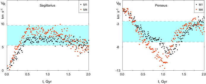
Figure 7: Variations of the radial residual velocity $V_{R}$ in the Sagittarius and Perseus complexes in model 1 and 4. The absolute values of the velocities $V_{R}$ are larger in model 4 than in model 1 what can be connected with the larger value of $Q_{T}$ in model 4 than in model 1 in the solar neighborhood.

Table 5 indicates that the residual velocities, $V_{R}$ and $V_{T}$, produced by models 1–3 are nearly the same while model 4 creates a bit larger velocity perturbations. This difference is especially noticeable in the distribution of velocities $V_{R}$ in the Sagittarius and Perseus complexes. To compare model 1 and 4 we build Figure 7 which shows the radial residual velocities $V_{R}$ produced by both models in the Sagittarius and Perseus complexes. The absolute values of the radial velocities $V_{R}$ are larger in model 4 than in model 1 what can be connected with the larger value of $Q_{T}$ in model 4 than in model 1 in the solar neighborhood (Fig. 3).

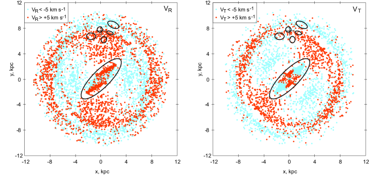
Figure 8: Distribution of OB particles with negative and positive residual velocities in model 1 at $t=1.5$ Gyr. The left and right panels represent the distribution of radial, $V_{R}$, and azimuthal, $V_{T}$, residual velocities, respectively. Particles with the conspicuous positive velocities ($V_{R}>+5$ or $V_{T}>+5$ km s^-1) are indicated as dark-gray circles (colored red in electronic edition) while those with the conspicuous negative velocities ($V_{R}<-5$ or $V_{T}<-5$ km s^-1) are shown as light-gray circles (colored blue in electronic edition). Particles with the residual velocities close to zero ($|V_{R}|<5$ or $|V_{T}|<5$ km s^-1) aren’t shown here. It also represents the boundaries of the Sagittarius, Carina, Cygnus, LS and Perseus stellar-gas complexes. The model galaxy is turned to rotate clockwise. The location of the complexes is determined for the solar position angle of $\theta_{b}=45^{\circ}$. The left panel indicates that the velocities $V_{R}$ of model particles are positive in the Sagittarius, Carina, Cygnus and LS stellar-gas complexes while they are negative in the Perseus complex. The right panel shows that the velocities $V_{T}$ are negative in the Perseus complex.

Figure 8 shows the distribution of OB particles with negative ($V_{res}<5$ km s^-1) and positive ($V_{res}>5$ km s^-1) residual velocities in model 1 at $t=1.5$ Gyr. Particles with the residual velocities close to zero ($|V_{res}|<5$ km s^-1) aren’t shown there. The left panel indicates that velocities $V_{R}$ of model particles are positive in the Sagittarius, Carina, Cygnus and Local System stellar-gas complexes while they are negative in the Perseus complex. The right panel shows that the velocities $V_{T}$ are negative in the Perseus complex.

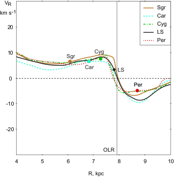
Figure 9: Variations of the radial residual velocities, $V_{R}$, along the Galactocentric distance, $R$, calculated for five Galactic radius-vectors connecting the Galactic center with the centers of the corresponding stellar-gas complexes: Sagittarius, Carina, Cygnus, Local System and Perseus. The position angle of the Sun with respect to the bar major axis is adopted to be $\theta_{b}=45^{\circ}$. The vertical line indicates the radius of the OLR. The model velocity $V_{R}$ at each point of the profiles is computed as the average velocity of model particles (gas+OB) located inside a small region with the radius of 0.5-kpc and the center lying on the corresponding radius-vector. Model 1 at $t=1.5$ Gyr is considered. All profiles demonstrate a sharp drop in the velocity $V_{R}$ at the distance of the OLR.

Figure 9 demonstrates the variations of the radial velocity $V_{R}$ along the distance $R$ calculated for five radius-vectors connecting the Galactic center with the centers of the corresponding stellar-gas complexes: Sagittarius, Carina, Cygnus, Local System and Perseus. These radius-vectors form a bit different angles with the Sun-Galactic center line: $\theta=4.0^{\circ}$ (Sgr), -13.3^∘ (Car), +11.0^∘ (Cyg), -1.6^∘ (LS) and 12.8^∘ (Per). The velocity $V_{R}$ at each point of the profiles is computed as the average velocity of model particles (gas+OB) located inside a small circle with the radius of 0.5-kpc and the center lying on the corresponding radius-vector. Model 1 at $t=1.5$ Gyr is considered. It is clear that all profiles demonstrate a sharp drop in the velocity $V_{R}$ at the distance of the OLR. Generally, we can shift the position of the OLR of the bar by choosing a different value of $\Omega_{b}$, but if we like the velocity $V_{R}$ in the Local System to be positive, then we would inevitably obtain positive $V_{R}$ in the Sagittarius, Carina and Cygnus complexes which are located at the smaller Galactocentric distances $R$ than that of the Local System. However, the observed velocities $V_{R}$ in the Carina and Cygnus complexes are negative (Table 1).

The uncertainty in a choice of the value of the angular velocity of the bar, $\Omega_{b}=50$ km s^-1 kpc^-1, is less than $\pm 2$ km s^-1 kpc^-1. If we choose $\Omega_{b}$ to be 52 km s^-1 kpc^-1 than the radius of the OLR will be shifted by 0.3 kpc toward the Galactic center and the average velocities $V_{R}$ in the Local System will be negative. On the contrary, the value of $\Omega_{b}=48$ km s^-1 kpc^-1 shifts the OLR by 0.3 kpc away from the Galactic center and causes the velocities $V_{T}$ in the Perseus region to be too small in absolute value, $|V_{T}|<3$ km s^-1. All these changes cause a discrepancy with observations.

Table 6 lists the average residual velocities of model particles, $V_{R}$ and $V_{T}$, located within the boundaries of the Carina and Cygnus stellar-gas complexes in model 1 at different time moments. Other models give similar results. The bottom line indicates the observed velocities. It is clear that present models cannot reproduce the observed velocities in the Carina and Cygnus complexes. Probably, some important physical processes which determine the kinematics just in these two regions aren’t included into consideration.

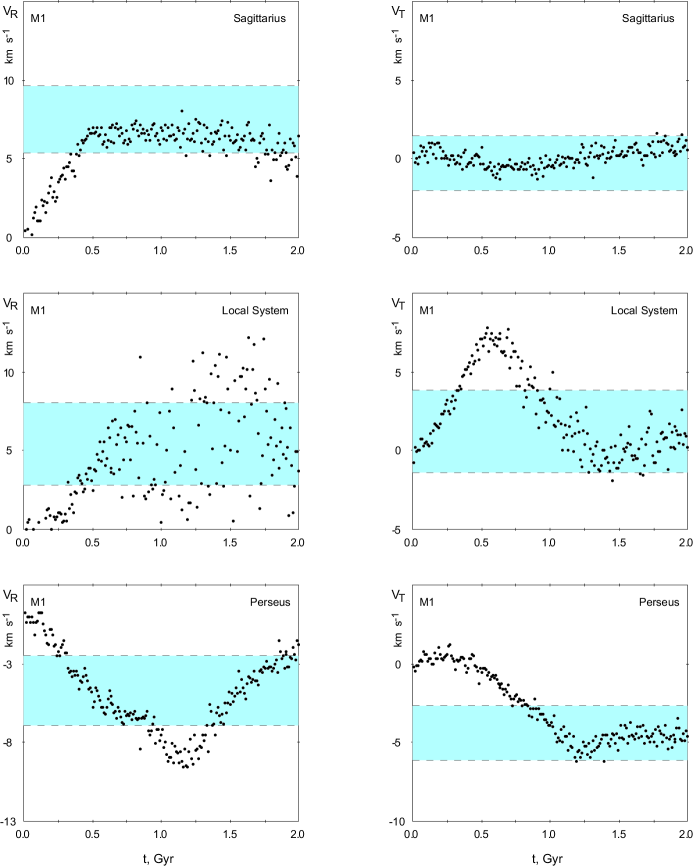
Figure 6: Comparison of model and observed residual velocities calculated for the three stellar-gas complexes: Sagittarius, Local System and Perseus. The left and right panels show radial and azimuthal, $V_{R}$ and $V_{T}$, residual velocities, respectively. The gray strips (colored blue in electronic edition) display the uncertainties in determination of observed residual velocities, $V_{obs}\pm\varepsilon_{v}$ (Table 1). Black circles indicate the average velocities of model particles (gas+OB) located inside the boundaries of stellar-gas complexes in model 1 every 10 Myr. The position angle of the Sun with respect to the bar is adopted to be $\theta_{b}=45^{\circ}$.

Table 5: Residual velocities, $V_{R}$ and $V_{T}$, calculated for the Sagittarius, Local System and Perseus stellar-gas complexes in models 1–4

Complex		Sagittarius			Local System			Perseus
Model	$t$	$V_{R}\quad$	$V_{T}\quad$	$n\;$	$V_{R}\quad\;$	$V_{T}\quad\;$	$n\;$	$V_{R}\quad\;$	$V_{T}\quad\;$	$n\;$
	Gyr	km s-1	km s-1		km s-1	km s-1		km s-1	km s-1
Model 1	0.7	$6.6\pm 0.1$	$-0.5\pm 0.1$	178	$5.1\pm 0.3$	$6.2\pm 0.2$	186	$-6.0\pm 0.1$	$-1.9\pm 0.1$	378
	0.9	$6.7\pm 0.1$	$-0.5\pm 0.1$	183	$4.1\pm 0.7$	$3.4\pm 0.2$	145	$-6.9\pm 0.2$	$-3.1\pm 0.1$	434
	1.1	$6.6\pm 0.1$	$-0.2\pm 0.1$	182	$2.5\pm 0.7$	$1.7\pm 0.3$	103	$-8.8\pm 0.1$	$-4.8\pm 0.2$	488
	1.3	$6.5\pm 0.1$	$0.2\pm 0.1$	184	$6.5\pm 0.7$	$-0.0\pm 0.2$	77	$-7.7\pm 0.2$	$-5.3\pm 0.1$	479
	1.5	$6.3\pm 0.1$	$0.4\pm 0.1$	182	$7.4\pm 0.9$	$-0.3\pm 0.2$	74	$-5.3\pm 0.2$	$-4.6\pm 0.1$	457
	1.7	$5.9\pm 0.2$	$0.6\pm 0.1$	184	$7.4\pm 0.7$	$0.1\pm 0.3$	79	$-3.7\pm 0.1$	$-4.5\pm 0.1$	452
	1.9	$5.4\pm 0.2$	$0.8\pm 0.1$	191	$5.0\pm 0.5$	$0.8\pm 0.2$	94	$-2.6\pm 0.1$	$-4.6\pm 0.1$	449
M2	0.7	$6.9\pm 0.1$	$-0.6\pm 0.1$	168	$5.8\pm 0.4$	$5.5\pm 0.2$	88	$-6.6\pm 0.2$	$-2.2\pm 0.1$	116
	0.9	$6.7\pm 0.2$	$-0.4\pm 0.1$	165	$4.9\pm 0.9$	$2.7\pm 0.2$	69	$-8.3\pm 0.3$	$-3.8\pm 0.1$	143
	1.1	$6.3\pm 0.1$	$-0.3\pm 0.1$	166	$2.5\pm 0.7$	$0.9\pm 0.3$	49	$-10.3\pm 0.2$	$-5.8\pm 0.2$	157
	1.3	$6.2\pm 0.1$	$-0.1\pm 0.1$	173	$7.4\pm 1.4$	$-1.0\pm 0.3$	38	$-9.7\pm 0.3$	$-6.7\pm 0.2$	163
	1.5	$6.2\pm 0.1$	$0.2\pm 0.1$	172	$8.4\pm 1.0$	$-1.4\pm 0.3$	34	$-5.7\pm 0.3$	$-5.9\pm 0.2$	147
	1.7	$5.8\pm 0.2$	$0.6\pm 0.1$	170	$7.9\pm 0.8$	$-1.0\pm 0.4$	39	$-3.8\pm 0.2$	$-6.1\pm 0.2$	148
	1.9	$5.2\pm 0.1$	$0.6\pm 0.1$	175	$6.6\pm 0.5$	$-0.3\pm 0.2$	46	$-1.7\pm 0.2$	$-6.1\pm 0.2$	150
M3	0.7	$6.6\pm 0.1$	$-0.3\pm 0.1$	182	$5.9\pm 0.3$	$5.8\pm 0.3$	182	$-5.8\pm 0.1$	$-1.8\pm 0.1$	372
	0.9	$6.5\pm 0.1$	$-0.3\pm 0.1$	184	$4.4\pm 0.8$	$3.2\pm 0.2$	144	$-6.9\pm 0.2$	$-3.1\pm 0.1$	429
	1.1	$6.7\pm 0.1$	$0.0\pm 0.1$	180	$2.9\pm 0.6$	$0.7\pm 0.2$	104	$-8.8\pm 0.2$	$-4.6\pm 0.1$	475
	1.3	$6.4\pm 0.1$	$0.2\pm 0.1$	185	$6.0\pm 0.8$	$-0.6\pm 0.3$	74	$-8.0\pm 0.2$	$-5.2\pm 0.1$	462
	1.5	$6.2\pm 0.1$	$0.7\pm 0.1$	185	$9.0\pm 0.7$	$-1.1\pm 0.2$	71	$-5.0\pm 0.2$	$-4.6\pm 0.1$	439
	1.7	$5.8\pm 0.2$	$1.1\pm 0.1$	190	$7.4\pm 0.4$	$-0.4\pm 0.2$	78	$-3.4\pm 0.1$	$-4.6\pm 0.1$	441
	1.9	$5.2\pm 0.2$	$1.2\pm 0.1$	190	$5.8\pm 0.3$	$0.1\pm 0.2$	93	$-2.0\pm 0.1$	$-4.8\pm 0.1$	441
M4	0.7	$8.4\pm 0.2$	$-0.7\pm 0.1$	174	$6.6\pm 0.5$	$5.4\pm 0.3$	171	$-8.3\pm 0.2$	$-2.9\pm 0.1$	385
	0.9	$8.2\pm 0.1$	$-0.1\pm 0.1$	175	$4.4\pm 0.8$	$2.7\pm 0.3$	122	$-10.3\pm 0.2$	$-4.9\pm 0.2$	470
	1.1	$8.2\pm 0.2$	$0.6\pm 0.1$	181	$4.5\pm 0.8$	$0.2\pm 0.3$	74	$-9.8\pm 0.3$	$-5.8\pm 0.1$	475
	1.3	$7.7\pm 0.2$	$1.1\pm 0.1$	191	$11.1\pm 0.7$	$-1.6\pm 0.4$	60	$-5.7\pm 0.2$	$-4.8\pm 0.1$	427
	1.5	$6.6\pm 0.2$	$1.5\pm 0.1$	194	$8.6\pm 0.7$	$-0.6\pm 0.2$	67	$-3.9\pm 0.2$	$-4.9\pm 0.1$	447
	1.7	$5.4\pm 0.2$	$1.3\pm 0.2$	188	$4.8\pm 0.6$	$1.3\pm 0.2$	88	$-2.9\pm 0.2$	$-5.1\pm 0.1$	437
	1.9	$5.2\pm 0.2$	$0.7\pm 0.1$	192	$2.5\pm 0.4$	$2.2\pm 0.2$	128	$-3.7\pm 0.2$	$-4.0\pm 0.1$	409
Observations		$7.5\pm 2.1$	$-0.3\pm 1.7$		$5.4\pm 2.6$	$1.2\pm 2.6$		$-4.7\pm 2.2$	$-4.4\pm 1.7$

Table 6: Residual velocities, $V_{R}$ and $V_{T}$, computed for the Carina and Cygnus stellar-gas complexes in model 1

Complex		Carina		Cygnus
$t$	$V_{R}\quad$	$V_{T}\quad$	$n\;$	$V_{R}\quad\;$	$V_{T}\quad\;$	$n\;$
Gyr	km s-1	km s-1		km s-1	km s-1
0.7	$6.1\pm 0.1$	$-2.5\pm 0.2$	282	$8.2\pm 0.2$	$9.0\pm 0.1$	217
0.9	$6.3\pm 0.1$	$0.6\pm 0.3$	326	$7.1\pm 0.4$	$8.9\pm 0.3$	153
1.1	$5.8\pm 0.1$	$3.0\pm 0.2$	345	$6.2\pm 0.4$	$6.7\pm 0.3$	110
1.3	$5.9\pm 0.2$	$2.2\pm 0.2$	320	$7.4\pm 0.4$	$4.1\pm 0.3$	106
1.5	$5.9\pm 0.1$	$0.2\pm 0.2$	304	$8.9\pm 0.3$	$3.0\pm 0.2$	103
1.7	$6.5\pm 0.1$	$-1.1\pm 0.1$	291	$9.4\pm 0.4$	$2.9\pm 0.1$	100
1.9	$6.7\pm 0.2$	$-1.2\pm 0.2$	282	$9.5\pm 0.3$	$2.5\pm 0.2$	96
Observations	$-6.2\pm 2.6$	$+6.2\pm 2.8$		$-4.3\pm 1.3$	$-10.3\pm 1.4$

4.2 Position angle of the Sun with respect to the bar major axis

In the previous analysis, the value of the position angle of the Sun with respect to the bar major axis was adopted to be $\theta_{b}=45^{\circ}$. This section gives some rationale of that choice. Figure 10 shows the dependence of the difference between model and observed residual velocities, $\Delta V_{R}$ and $\Delta V_{T}$:

$$\Delta V_{R}=V_{R\;mod}-V_{R\;obs},$$ (10)

$$\Delta V_{T}=V_{T\;mod}-V_{T\;obs}$$ (11)

on the position angle $\theta_{b}$. The model residual velocities are determined as average residual velocities in model 1 at the time interval 1.4–1.6 Gyr. The strips show the intervals of permissable deviations between model and observed velocities which are adopted to be $\pm 2.5$ km s^-1 representing the average uncertainty in determination of observed velocities (Table 1). If a curve indicating values of $\Delta V_{R}$ or $\Delta V_{T}$ in some complex lies inside the corresponding strip then the model and observed velocities are consistent within the errors there.

Figure 10 (left panel) demonstrates that model and observed velocities $V_{R}$ in the Sagittarius, LS and Perseus stellar-gas complexes agree within the errors under the position angle $\theta_{b}$ lying in the range 33–52^∘. Note that the best agreement between model and observed velocities $V_{R}$ in the Sagittarius complex corresponds to $\theta_{b}\approx 45^{\circ}$. The Carina and Cygnus complexes show a large discrepancy between model and observed velocities for all values of $\theta_{b}$ from the interval considered.

The most interesting feature in variations of the azimuthal velocity $V_{T}$ concerns the Sagittarius complex. Figure 10 (right panel) indicates that model and observed velocities $V_{T}$ in the Sagittarius complex are consistent within the errors for $\theta_{b}>40^{\circ}$. On the contrary, the curve built for the Carina complex suggests that model and observed velocities agree for $\theta_{b}<40^{\circ}$ there. Note that model velocities $V_{T}$ in the Local System and Perseus complexes aren’t sensitive to the choice of $\theta_{b}$ and agree with observed velocities for any $\theta_{b}$ from the interval considered.

Thus, the model and observed velocities, $V_{R}$ and $V_{T}$, in the three stellar-gas complexes (Sagittarius, LS and Perseus) agree within the errors for the position angle $\theta_{b}$ lying at the interval 40–52^∘.

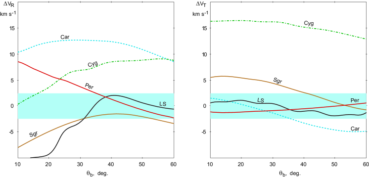
Figure 10: Dependence of the differences between model and observed velocities, $\Delta V_{R}$ and $\Delta V_{T}$, on the position angle $\theta_{b}$ of the bar calculated for five stellar-gas complexes: Sagittarius, Carina, Cygnus, Local System (LS) and Perseus. The left and right panels show variations of the radial and azimuthal, $V_{R}$ and $V_{T}$, residual velocities, respectively. The gray strips (colored blue in electronic edition) display the permissable intervals of deviations between model and observed velocities which are adopted to be $\pm 2.5$ km s^-1. If a curve indicating values of $\Delta V_{R}$ or $\Delta V_{T}$ in some complex lies inside the strip then model and observed velocities are consistent within the errors there.

4.3 Surface-density profiles

The formation of the resonance rings can be traced by the surface-density profiles. Figure 11 shows the variations of the surface density $\Sigma$ of model particles (gas+OB) along the Galactocentric distance $R$ built for models 1–4 at four time moments: $t=0.0$, 0.5, 1.0 and 1.5 Gyr. These profiles clearly indicate the positions of the resonance rings.

The nuclear rings ($n$) are forming between the two ILRs at the distance of $R=0.2\textrm{--}0.9$ kpc (Fig. 11). The surface density of the nuclear rings achieves maximum at the time moment $t\sim 0.5$ Gyr and then starts decreasing. This process goes most quickly in model 2 that can be due to the largest frequency of collisions there.

The inner rings ($r$) are growing at the distance of $R=3.0\textrm{--}3.3$ kpc which is a bit larger than that of the 4/1 resonance. Note that an inner ring is practically absent in model 4 – we can see only a small density enhancement at $t=0.5$ Gyr there. Interestingly, the conspicuous diamond-shape structures inside the Ferrers ellipsoid visible in many frames of Figure 4 at the distances 1–3 kpc appears to lie in the region with the reduced surface density (Fig. 11).

The outer rings, $R_{1}$ and $R_{2}$, are emerging at the distances 6.7–7.3 and 8.5–9.3 kpc, respectively (Fig. 11). They get maximum $\Sigma$ at the interval $t=1.0\textrm{--}1.5$ Gyr, though the rings $R_{2}$ grow a bit slower. The surface density enhancements above the background are nearly the same in two outer rings. However, the rings $R_{2}$ are nearly twice wider than $R_{1}$ in all models what suggests that the rings $R_{2}$ manage to catch twice more particles than the rings $R_{1}$.

On the whole, the positions and growth rate of the resonance rings in models considered agree with the estimates obtained in previous simulations (Schwarz, 1981; Byrd et al., 1994; Buta & Combes, 1996; Rautiainen & Salo, 1999, 2000; Melnik & Rautiainen, 2009; Rautiainen & Melnik, 2010).

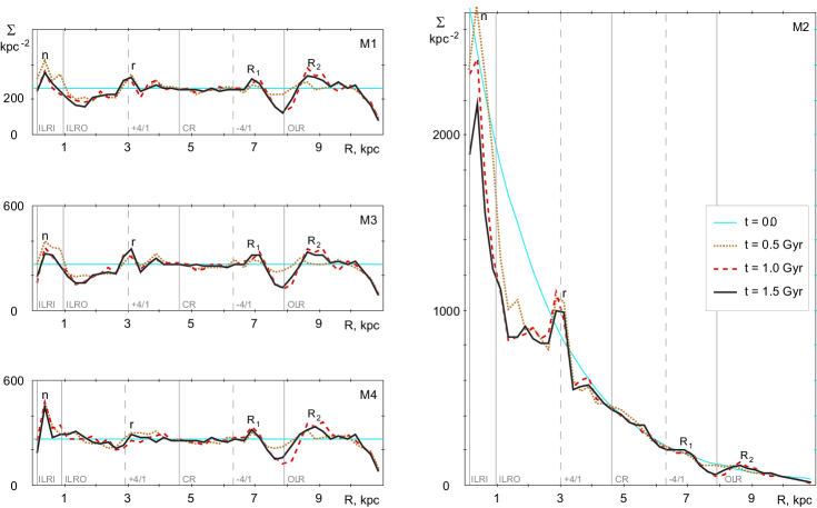
Figure 11: Profiles of the surface density $\Sigma$ built for the distribution of model particles (gas+OB) in models 1–4 at several time moments: $t=0.0$, 0.5, 1.0 and 1.5 Gyr. Density maxima related to the resonance rings are designated by letters: $n$ – nuclear rings, $r$ – inner rings, $R_{1}$ and $R_{2}$ – outer rings. The locations of the resonances are also indicated. The profile built for model 2 exhibits a larger range of density variations but the scale is the same in all frames. We can see that the nuclear rings achieve maximum density at the time moment $t=0.5$ Gyr while the outer rings get maximum $\Sigma$ at the interval $t=1.0\textrm{--}1.5$ Gyr. The surface density excesses above the background are nearly the same in two outer rings but the rings $R_{2}$ are nearly twice wider than $R_{1}$ in all models. This suggests that the rings $R_{2}$ manage to catch twice more particles than $R_{1}$.

4.4 Velocity dispersion

The velocity perturbations from the bar give rise to both systematic motions and velocity dispersions. To separate the random and systematic velocities we divide model discs into annuli of 0.5-kpc width and then make a partition of every annulus into cells of $\sim$0.5-kpc length in azimuthal direction. Different annuli contain different numbers of cells. The velocities of model particles inside every cell are assumed to obey a linear law:

$$V_{R}=V_{1}+A_{1}(R-R_{c})+B_{1}(\theta-\theta_{c})+\xi,$$ (12)

$$V_{T}=V_{2}+A_{2}(R-R_{c})+B_{2}(\theta-\theta_{c})+\eta,$$ (13)

where $R_{c}$ and $\theta_{c}$ are the Galactocentric radius and Galactocentric angle of the center of a cell, $V_{1}$ and $V_{2}$ are the average velocities of model particles (gas+OB) in the cell in the radial and azimuthal directions, respectively; the parameters $A_{1}$, $B_{1}$, $A_{2}$ and $B_{2}$ describe the changes of systematic velocities in radial and azimuthal directions, while values $\xi$ and $\eta$ characterize the random deviations from the linear law. In the first approximation, the standard deviations of values $\xi$ and $\eta$ in every cell represent the velocity dispersions in radial and azimuthal directions, $\sigma_{R}$ and $\sigma_{T}$, respectively. The average values of $\sigma_{R}$ and $\sigma_{T}$ calculated for all cells located in the same annulus give us a smooth distribution of the velocity dispersion along the Galactocentric radius.

Figure 12 shows the changes of the velocity dispersion $\sigma_{R}$ along the Galactocentric distance $R$ in model 1 at different time moments. We can see the fast growth of $\sigma_{R}$ at the time interval 0.5–1.4 Gyr with maximal value of 23 km s^-1 being achieved at the radius of $\sim 8$ kpc, but then $\sigma_{R}$ declines by 15 km s^-1. All models demonstrate the similar growth and decline in $\sigma_{R}$. Probably, it is the process of the formation of the outer rings that is responsible for the extra increase of the velocity dispersion $\sigma_{R}$ at the time interval 1.0–1.4 Gyr. We merely cannot separate properly systematic and random motions during this process. The drop of $\sigma_{R}$ by the end of simulation is due to decreasing systematic motions which decline especially fast in the ring $R_{2}$ (see variations of $V_{R}$ in the Perseus region, Figure 6, Table 5). Generally, the value of 15 km s^-1 can be considered as the upper estimate of $\sigma_{R}$ at the radius of the OLR.

Note that Figure 12 exhibits the velocity dispersion at the interval of Galactocentric distances from 4 to 11 kpc only. In the central region the velocity dispersion achieves considerably higher values. For example, at the distance of the nuclear ring, $R\approx 0.5$ kpc, $\sigma_{R}$ reaches $\sim 100$ km s^-1.

The velocity dispersion $\sigma_{T}$ is growing at the time interval 0.5–1.4 Gyr and amounts to 10 km s^-1, which is nearly twice smaller than maximum of $\sigma_{R}$, but then $\sigma_{T}$ decreases by the value of 7 km s^-1.

Figure 13(a) shows the radial oscillations of two model particles which appear to lie inside the Local System in model 3 (one without collisions) at the time moment $t=1.5$ Gyr. Chosen particles represent oscillations going in opposite phases. The growth of the amplitudes evidences the resonance. Figure 13(b) demonstrates the variations of the specific angular momentum $L$ and will be discussed in section 4.5. Figures 13(c) and 13(d) represent the orbits of these particles in the reference frame corotating with the bar. We can see that particle 1 supports the outer ring $R_{1}$ while particle 2 supports the ring $R_{2}$. Note that particle 1 has the positive radial velocity $V_{R}$ at $t=1.5$ Gyr, when it lies inside the Local System, while particle 2 has the negative velocity $V_{R}$ at the same moment.

Figure 13(a) indicates that particle 1 has a maximal amplitude of radial oscillations at $t=0.9$ Gyr approaching the distances of 6.9 and 8.4 kpc but then the oscillations start fading. Particle 2 deviates considerably from its initial radius, $R=7.5$ kpc, approaching the distances of 10.0 and 6.8 kpc. Moreover, the deviations of particle 2 in the direction away from the Galactic center are larger than those in the opposite direction suggesting the increase of its average distance $R$.

Figure 13(d) shows that the orbit of particle 2 first isn’t aligned with the bar being stretched at the angle of $\sim 45^{\circ}$ with respect to the bar major axis and taking an intermediate position between the orientations of orbits in the ring $R_{1}$ and $R_{2}$. However, the orbit has got the right orientation being elongated along the bar by the time $t=1.5$ Gyr. This adjustment of orbits causes the changes in both systematic velocities and velocity dispersions.

There is a question whether such large values of the velocity dispersion $\sigma_{R}$ emerging near the OLR agree with observations. The velocity dispersion $\sigma_{R}$ achieves large values, $\sigma_{R}\approx 15$ km s^-1, at the small interval of Galactocentric distances 7.5–8.5 kpc. However, this interval corresponds to minimum in the distribution of the surface density of model particles (Fig. 11). Probably, the number of particles with large velocity dispersion is not large. To check that we selected OB-particles located within 3 kpc from the adopted solar position ($R_{0}=7.5$ kpc, $\theta_{b}=45^{\circ}$) and derived the parameters of the rotation curve and velocity dispersion from model velocities. Here we supposed that model particles move in circular orbits in accordance with Galactic differential rotation. The same method was applied to observational data (Melnik & Dambis, 2009). The derived rotation curve appears to be in good agreement with the observed rotation curve. The standard deviation $\sigma_{v}$ of the velocities of OB-particles from the rotation curve computed jointly for radial and azimuthal directions proves to be 11 km s^-1 (model 1, $t=1.5$ Gyr). It is a bit larger than $\sigma_{v}$ obtained for observed OB-associations (7–8 km s^-1, Melnik & Dambis, 2017) but still smaller than $\sigma_{v}$ calculated for young open clusters (15 km s^-1, Melnik et al., 2016) and close to $\sigma_{v}$ derived for classical Cepheids (10–11 km s^-1, Melnik et al., 2015). The fraction of particles with $|V_{R}|>15$ km s^-1 appears to be only 7 per cent but their exclusion decreases the velocity dispersion to the value of $\sigma_{v}=6$ km s^-1.

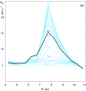
Figure 12: Dependence of the velocity dispersion $\sigma_{R}$ on the galactocentric radius $R$ in model 1 at time moments $t$ from $t=0$ to 2.0 Gyr every 0.1 Gyr time interval. The profile related to $t=2.0$ Gyr is distinguished by the thick black line while other profiles are depicted by the thin gray lines (colored blue in electronic edition). Numbers near some profiles indicate the time moments in Gyr. The velocity dispersion $\sigma_{R}$ achieves maximum at the radius of $\sim 8$ kpc at the time moment $t=1.4$ Gyr but then it starts decreasing. All values of $\sigma_{R}$ located above the value of 15 km s^-1 can be considered as overestimated due to contribution of systematic radial velocities.

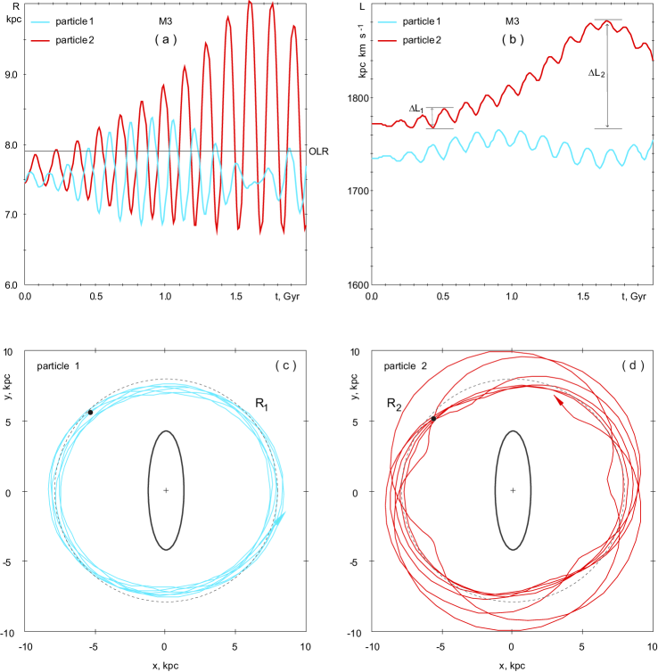
Figure 13: (a) Radial oscillations of two model particles (model 3) which appear to lie inside the Local System at the time moment $t=1.5$ Gyr. The oscillations of particle 1 (colored blue in electronic edition) and particle 2 (colored red in electronic edition) support the outer ring $R_{1}$ and $R_{2}$, respectively. (b) Variations of the specific angular momentum $L$ of two chosen particles. (c) Orbit of particle 1 in the reference frame corotating with the bar. The ellipse indicates the position of the bar. The thin dash line shows the radius of the OLR. A black circle in the upper left corner points the position of the particle at $t=1.5$ Gyr. (d) Orbit of particle 2 in the reference frame corotating with the bar (see details above).

4.5 Distribution of the angular momentum

The rotation of the bar in the galactic discs causes the redistribution of the specific angular momentum $L$:

$$L=\Theta R$$ (14)

along the Galactocentric distance $R$, where $\Theta$ is the velocity in the azimuthal direction.

So far we have considered the kinematics near the OLR of the bar only but in this section it makes sense to study motions near both Lindblad resonances: ILR and OLR. The redistribution of the angular momentum $L$ near both Lindblad resonances seems to have one physical reason.

Figure 14(a) shows the distribution of the azimuthal velocities $\Theta$ of model particles (gas+OB) averaged in thin annuli of 40-pc width along the Galactocentic distance $R$ in model 1 at $t=1.5$ Gyr. Also shown is the velocity of the rotation curve, $V_{c}$, which reflects the initial distribution of $\Theta$. We can see that particles located near the ILR and OLR of the bar change their velocity $\Theta$ in a similar way forming a hump and a pit near the radius of the resonance. The average azimuthal velocity $\Theta$, and consequently $L$, increases (decreases) at the radii a bit smaller (larger) than those of the Lindblad resonances. In the neighborhood of the ILR, the velocity $\Theta$ grows at the distance of the nuclear ring and decreases in the region of most populated bar orbits. In the vicinity of the OLR, the velocity $\Theta$ increases and decreases at the distances of the ring $R_{1}$ and $R_{2}$, respectively. Figure 14(b) demonstrates the distribution of the specific angular momentum $L$ of model particles averaged in thin annuli. The initial distribution of $L$ is also indicated. It is seen that the most significant changes of $L$ occur in the bar region. Note that all models demonstrate similar behavior.

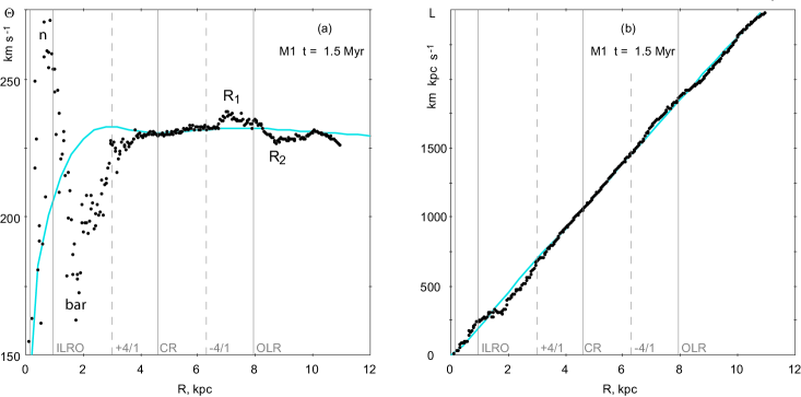
Figure 14: (a) Distribution of the azimuthal velocity $\Theta$ (black circles) of model particles (gas+OB) averaged in thin annuli of 40-pc width along the Galactocentic radius $R$ in model 1 at $t=1.5$ Gyr. The gray line (colored blue in electronic edition) shows the velocity of the rotation curve, $V_{c}$, which reflects the initial distribution of $\Theta$. The vertical gray lines indicate the positions of the resonances. We can see that the average azimuthal velocity $\Theta$, and consequently $L$, increases in the nuclear region (n) and in the $R_{1}$-region while $\Theta$ and $L$ decrease in the bar region and in the $R_{2}$-region. (b) Distribution of the specific angular momentum $L$ (circles) of model particles averaged in thin annuli of 40-pc width along the distance $R$. The gray line (colored blue in electronic edition) indicates the initial distribution of $L$. The most significant changes of $L$ occur in the bar region.

As the bar creates accelerations in azimuthal direction, the angular momentum $L$ isn’t conserved in barred galaxies. However, most of particles on their quasi-periodic orbits acquire and lose nearly the same value of angular momentum, $\Delta L$, during their revolution with respect to the bar.

Figure 13(b) presents the oscillations of the specific angular momentum of the two particles supporting the outer ring $R_{1}$ and $R_{2}$. We can see fast oscillations of the angular momentum, $\Delta L_{1}$, with the period of $\sim 150$ Myr corresponding to a half of their revolution period with respect to the bar. The range (twice amplitude) of these changes is $\Delta L_{1}\approx 20$ km kpc s^-1. Besides the fast oscillations we can see slower ones. For example, particle 2 increases its angular momentum by the value of $\Delta L_{2}\approx 100$ km kpc s^-1 during the formation of the ring $R_{2}$ at the time interval 1–1.5 Gyr. However, both these values correspond to quite small changes of $R$. Figure 14(b) demonstrates nearly linear growth of the angular momentum $L$ with increasing $R$. Using Eq. 14 and the value of $\Theta=232$ km s^-1 we can estimate the variations in $R$ corresponding to $\Delta L_{1}$ and $\Delta L_{2}$ which appear to be $\Delta R_{1}=0.1$ and $\Delta R_{2}=0.4$ kpc, respectively. Both these values are small in comparison with the range (twice amplitude) of radial oscillations of particle 1 and 2 equal to $\Delta R=1.5$ and 3.2 kpc, respectively (Fig. 13a). Thus, model particles show only small variations of $L$ during their radial oscillations.

The resonance amplifies epicyclic motions and throws particles to the distances corresponding to larger changes of their angular momenta than $\Delta L_{1}$ and $\Delta L_{2}$ received from the bar. Particles from smaller distances $R$ having smaller angular momenta $L$ can come to larger distances at which particles initially have larger $L$ and vice versa. So the average value of the azimuthal velocity $\Theta$ and $L$ decreases (increases) at the radii a bit larger (smaller) than those of the Lindblad resonances.

Probably, the redistribution of $L$ near the Lindblad resonances of the bar is due to the existence of elongated periodic orbits which catch a lot of particles from nearby space. The residual azimuthal velocities $V_{T}$ are directed in the opposite senses at the apocenters (outermost points) and pericenters (innemost points) of periodic orbits.

Figure 15 shows the directions of the residual velocities at different points of periodic orbits supporting the nuclear ring, bar and outer rings. The additional (residual) azimuthal velocity $V_{T}$ is directed in the sense opposite that of galactic rotation ($V_{T}<0$) at the apocenters ($A$, $A^{\prime}$, $F$, $F^{\prime}$, $C$ and $C^{\prime}$) of elongated periodic orbits while $V_{T}$ is directed in the sense of galactic rotation ($V_{T}>0$) at the pericenters ($E$, $E^{\prime}$, $B$, $B^{\prime}$, $D$ and $D^{\prime}$). The radial velocity $V_{R}$ gets its extreme values at the points lying at about $\pm 45^{\circ}$-angles with respect to the bar axes.

Probably, the tuning of epicyclic motions (Fig. 15) causes the appearance of annuli with deficiency and excess of angular momentum $L$. These annuli must be located at some distances away from the Lindblad resonances, because precisely at the radii of the resonances, there are both pericenters and apocenters of periodic orbits oriented perpendicular to each other there. For example, we can see that the apocenters ($F$ and $F^{\prime}$) and pericenters ($E$ and $E^{\prime}$) of periodic orbits existing near the OLR are located practically at the radius of the OLR, so the average value of the azimuthal velocity $\Theta$ must be close to that of the rotation curve there. But at some distances away from the Lindblad resonances there is nothing to compensate the systematic changes in the azimuthal velocity. The deficiency of $L$ ($V_{T}<0$) corresponds to the apocenters ($A$, $A^{\prime}$, $C$ and $C^{\prime}$) of periodic orbits oriented along the bar while the excess of $L$ ($V_{T}>0$) occurs at the pericenters ($B$, $B^{\prime}$, $D$ and $D^{\prime}$) of periodic orbits elongated perpendicular to the bar. Thus, the redistribution of $L$ along the radius is caused by the existence of two types of stable periodic orbits elongated perpendicular to each other near the Lindblad resonances of the bar.

Let us imagine the motions of two particles located near the points E and F at some moment and call them, for simplicity, particle E and F, respectively (Fig. 15). Due to galactic differential rotation, particle E lying at a bit larger $R$ must rotate with a bit smaller angular velocity $\Omega$ than particle F. So particle E must drift counterclockwise in the azimuthal direction with respect to particle F. However, the epicyclic motions adjusted by the resonance can slow down or even change the direction of this drift. The velocity $V_{T}$ at the point E is directed in such a way to increase $\Omega$ while $V_{T}$ at the point F must decrease $\Omega$. Thus, the resonance can cause the rotation of particle E and F with the same angular velocity for some time period. This co-rotation doesn’t affect velocities of test particles in models without self-gravity, as it is in the case considered. But if self-gravity is included, then this co-motion can create favorite conditions for the growth of overdensities (Julian & Toomre, 1966; Toomre, 1981; Sellwood & Kahn, 1991) and the formation of slow modes (Rautiainen & Salo, 2000; Rautiainen & Melnik, 2010; Melnik & Rautiainen, 2013).

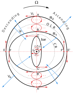
Figure 15: Schematic description of epicyclic motions at different points of periodic orbits supporting the nuclear ring ($n$), bar, outer ring $R_{1}$ and $R_{2}$. The additional velocity $V_{T}$ due to epicyclic motions (colored red in electronic edition) is directed in the sense opposite that of galactic rotation at the apocenters ($A$, $A^{\prime}$, $F$, $F^{\prime}$, $C$ and $C^{\prime}$) of periodic orbits and in the sense of galactic rotation at the pericenters ($E$, $E^{\prime}$, $B$, $B^{\prime}$, $D$ and $D^{\prime}$). The radial velocity $V_{R}$ (colored blue in electronic edition) gets extreme values at the points lying at about $\pm 45^{\circ}$-angles with respect to the bar axes. The Galaxy rotates clockwise but in the reference frame corotating with the bar objects located outside the CR, including those related to the outer rings, are moving counterclockwise. The Sun is supposed to lie at $\theta_{b}=45^{\circ}$ with respect to the bar major axis near the descending segment ($V_{R}<0$) of the ring $R_{2}$.

5 Conclusions

We studied models with analytical Ferrers bars and compared velocities of model particles with the observed velocities of OB-associations. Two power indexes in the density distribution inside the Ferrers ellipsoids were considered: $n=2$ (models 1–3) and $n=1$ (model 4). The initial surface-density distribution of model particles is exponential in model 2 and uniform in other models. Model 3 doesn’t include collisions but in other models particles can collide with each other inelastically.

All models considered can reproduce the observed residual velocities (those after subtraction of the velocities due to the rotation curve and the solar motion towards the apex) of OB-associations in the Sagittarius, Local System and Perseus stellar-gas complexes. There are a lot of moments at the time interval 1–2 Gyr after the start of simulations when model and observed velocities agree within the errors (Fig. 6).

The success in reproduction of the velocities in the Local System is due to the large velocity dispersion of model particles which weakens the resonance effects by producing smaller systematic velocity changes.

The model and observed residual velocities in the Sagittarius, Local System and Perseus stellar-gas complexes agree within the errors under the solar position angle $\theta_{b}=40\textrm{--}52^{\circ}$ (Fig. 10).

The angular velocity of the bar is adopted to be $\Omega_{b}=50$ km s^-1 kpc^-1 which corresponds to the location of the OLR of the bar 0.4 kpc outside the solar circle, $R_{OLR}=R_{0}+0.4$ kpc. The uncertainty in determination of $\Omega_{b}$ is less than $\pm 2$ km s^-1 kpc^-1.

Model galaxies form nuclear, inner and outer resonance rings. The nuclear rings appear between the two ILRs at the distance $\sim 0.5$ kpc from the center. The inner rings are growing at the radius of $\sim 3.3$ kpc which is a bit larger than that of the 4/1 resonance. The outer rings, $R_{1}$ and $R_{2}$, are forming at the radii of $\sim 7.0$ and $\sim 8.8$ kpc, respectively. The surface density excess is nearly the same in two outer rings. However, the rings $R_{2}$ are nearly twice wider than $R_{1}$ in all models what means that the rings $R_{2}$ manage to catch twice more particles than $R_{1}$ (Fig. 11).

The dispersion of radial velocities, $\sigma_{R}$, never drops below 5 km s^-1 in models considered. It shows conspicuous growth at the radius of the OLR getting maximal value of 23 km s^-1 at 1.4 Gyr but then declines by 15 km s^-1. The extra growth of the velocity dispersion near the OLR seems to be connected with the difficulty in separation between systematic and random motions during the formation of the outer ring $R_{2}$ (Fig. 12).

Model particles demonstrate the redistribution of the specific angular momentum $L$ near the ILR and OLR of the bar (Fig. 14). The average value of the azimuthal velocity $\Theta$ and consequently $L$ increases (decreases) at the radii a bit smaller (larger) than those of the Lindblad resonances. The most significant changes of $L$ occur in the bar region. Probably, the redistribution of $L$ along the radius is caused by the existence of two types of stable periodic orbits elongated perpendicular to each other near the Lindblad resonances of the bar (Fig. 15).

6 acknowledgements

I thank the anonymous referee for fruitful discussion. I thank P. Rautiainen and A. K. Dambis for useful remarks and suggestions. This work has made use of data from the European Space Agency (ESA) mission Gaia (https://www.cosmos.esa.int/gaia), processed by the Gaia Data Processing and Analysis Consortium (DPAC, https://www.cosmos.esa.int/web/gaia/dpac/consortium). Funding for the DPAC has been provided by national institutions, in particular the institutions participating in the Gaia Multilateral Agreement.

References

- Antoja et al. (2018) Antoja T., Helmi A., Romero-Gomez M. et al., 2018, Nature, 561, 360
- Athanassoula (1984) Athanassoula E., 1984, Phys. Rep., 114, 321
- Athanassoula (1992) Athanassoula E., 1992, MNRAS, 259, 328
- Athanassoula (2005) Athanassoula E., 2005, MNRAS, 358, 1477
- Athanassoula et al. (1983) Athanassoula E., Bienayme O., Martinet L., Pfenniger D., 1983, A&A, 127, 349
- Athanassoula et al. (2009) Athanassoula E., Romero-Gómez M., Masdemont J. J., 2009, MNRAS, 394, 67
- Athanassoula & Sellwood (1986) Athanassoula E., Sellwood J. A., 1986, MNRAS, 221, 213
- Baba et al. (2009) Baba J., Asaki Y., Makino J., Miyoshi M., Saitoh T. R., Wada K., 2009, ApJ, 706, 471
- Baba et al. (2013) Baba J., Saitoh T. R., Wada K., 2013, ApJ, 763, 46
- Benjamin et al. (2005) Benjamin R. A., Churchwell E., Babler B. L. et al., 2005, ApJ, 630, L149
- Bertin & Lin (1996) Bertin G., Lin C. C., 1996, Spiral Structure in Galaxies: A Density Wave Theory, Cambridge, MA: MIT Press
- Binney & Tremaine (1987) Binney J., Tremaine S., Galactic Dynamics, Princeton Univ. Press, Princeton, New Jersey, 1987.
- Blaha & Humphreys (1989) Blaha C., Humphreys R. M., 1989, AJ, 98, 1598
- Block et al. (2001) Block D. L., Puerari I., Knapen J. H. et al., 2001, A&A, 375, 761
- Bobylev & Bajkova (2018) Bobylev V. V., Bajkova A. T., 2018, Astron. Lett. 44, 676
- Boehle et al. (2016) Boehle A., Ghez A. M., Schödel R. et al., 2016, ApJ, 830, 17
- Brahic & Henon (1977) Brahic A., Henon M., 1977, A&A, 59, 1
- Branham (2017) Branham R. L., 2017, Ap&SS, 362, 29
- Bressan et al. (2012) Bressan A., Marigo P., Girardi L. et al., 2012, MNRAS, 427, 127
- Brown et al. (2018) Brown A. G. A., Vallenari A., Prusti T. et al., 2018, A&A, 616, A1
- Buta (1995) Buta R., 1995, ApJS, 96, 39
- Buta (2017) Buta R., 2017, MNRAS, 471, 4027
- Buta & Combes (1996) Buta R., Combes F., 1996, Fund. Cosmic Physics, 17, 95
- Buta & Crocker (1991) Buta R., Crocker D. A., 1991, AJ, 102, 1715
- Buta, Laurikainen & Salo (2004) Buta R., Laurikainen E., Salo H., 2004, AJ, 127, 279
- Byrd et al. (1994) Byrd G., Rautiainen P., Salo H., Buta R., Crocker D. A., 1994, AJ, 108, 476
- Cabrera-Lavers et al. (2007) Cabrera-Lavers A., Hammersley P. L., González-Fernández C. et al., 2007, A&A, 465, 825
- Churchwell et al. (2009) Churchwell E., Babler B. L., Meade M. R. et al., 2009, PASP, 121, 213
- Combes & Sanders (1981) Combes F., Sanders R. H., 1981, A&A, 96, 164
- Comeron et al. (2014) Comerón S., Salo H., Laurikainen E. et al., 2014, A&A, 562, 121
- Contopoulos & Grosbol (1989) Contopoulos G., Grosbol P., 1989, A&AR, 1, 261
- Contopoulos & Papayannopoulos (1980) Contopoulos G., Papayannopoulos Th., 1980, A&A, 92, 33
- Dambis et al. (2013) Dambis A. K., Berdnikov L. N., Kniazev A. Y. et al., 2013, MNRAS, 435, 3206
- Debattista & Sellwood (2000) Debattista V. P., Sellwood J. A., 2000, ApJ, 543, 704
- Dehnen & Binney (1998) Dehnen W., Binney J., 1998, MNRAS, 294, 429
- de Vaucouleurs & Freeman (1972) de Vaucouleurs G., Freeman K. C., 1972, Vis. in Astron., 14, 163
- Díaz-García et al. (2016) Díaz-García S., Salo H., Laurikainen E., Herrera-Endoqui M., 2016, A&A, 587, 160
- D’Onghia et al. (2013) D’Onghia E., Vogelsberger M., Hernquist L., 2013, ApJ, 766, 34
- Dwek et al. (1995) Dwek E., Arendt R. G., Hauser M. G. et al., 1995, ApJ, 445, 716
- Efremov & Sitnik (1988) Efremov Yu. N., Sitnik T. G., 1988, Soviet Astron. Lett., 14, 347