Decoherence Entails Exponential Forgetting in Systems Complying with the Eigenstate Thermalization Hypothesis

Abstract

According to the eigenstate thermalization ansatz, matrices representing generic few body observables take on a specific form when displayed in the eigenbasis of a chaotic Hamiltonian. We examine the effect of environmental induced decoherence on the dynamics of observables that conform with said eigenstate thermalization ansatz. The obtained result refers to a description of the dynamics in terms of an integro-differential equation of motion of the Nakajima-Zwanzig form. We find that environmental decoherence is equivalent to an exponential damping of the respective memory kernel. This statement is formulated as rigorous theorem. Furthermore the implications of the theorem on the stability of exponential dynamics against decoherence and the transition towards Zeno-Freezing are discussed.

I Introduction

Coupling to some environment drives the local density matrix of a quantum system towards a diagonal form in a specific basis - this well known finding is at the heart of open quantum system theory Breuer et al. (2002). If this influence is such that its sole effect is to erase off-diagonal elements in the specific basis but leave diagonal elements unchanged, the process is sometimes called pure decoherence or pure dephasing Joos et al. (2013); Zurek (2003); Skinner and Hsu (1986); Alicki (2004). The (not necessarily orthogonal) basis states of the eventually diagonal density matrix correspond to “pointer states”. They are singled out by “environment induced superselection” and depend strongly on the observables through which a system couples to its environment. Some sort of decoherence is almost inevitably induced by any complex environment Esposito and Gaspard (2003), specific pointer states come with environments that may be thought of as monitoring some system observable, the pointer states then essentially being the eigenstates of the monitored observable. In both cases the decoherence process is routinely modeled by corresponding quantum master equations, often of Lindblad form Breuer et al. (2002). Environmental decoherence may in general alter the dynamics of any system observable substantially.

Somewhat more recent but similarly intensely debated is the eigenstate thermalization hypothesis (ETH) Deutsch (1991); Srednicki (1999); Rigol et al. (2008). Most encompassing the ETH may be described as a statement on the properties of the matrix elements $\langle l|A|m\rangle$ of some observable $A$ when represented in the energy eigenbasis $\{|l(m)\rangle\}$. According to the ETH ansatz, the diagonal elements are very similar when corresponding to similar energies, whereas the off-diagonal elements closely resemble a set of independent Gaussian random numbers, with zero mean and variances that smoothly depend on the position of the matrix element within the matrix. While rigorous conditions under which the ETH ansatz applies are yet unknown, there are plenty of numerical examples which confirm its applicability to standard observables in interacting many-body systems D’Alessio et al. (2016); Beugeling et al. (2015); Mondaini and Rigol (2017); D’Alessio et al. (2016). Generally validity of the ETH is expected for few-body observables in non-integrable systems. As one consequence of the ETH, expectation values effectively (up to Poincare recurrences) dynamically relax towards their equilibrium values as calculated from the respective ensembles (canonical, microcanonical, generalized Gibbs, etc.) The ETH, however, also entails a certain property of the actual relaxation behavior itself: It appears that if the ETH ansatz applies, a common relaxation behavior of the expectation value results, for a multitude of initial states $\ket{\psi_{k}(0)}$, i.e. $\langle\psi_{k}(0)|A(t)\psi_{k}(0)\rangle\approx\langle\psi_{k}(0)|A(0)\psi_{k}(0)\rangle g(t)$. ($g(t)$ is essentially given by the respective correlation function $g(t)\propto\langle A(t)A\rangle$) Srednicki (1999); Richter et al. (2018). This statement includes also and especially initial states far from equilibrium. While the statement itself and the concrete range of its validity are currently under scrutiny, we somewhat boldly move ahead with this this work and focus on the principles that arise if the validity is taken for granted (for a class of states to be defined below) and combined with the decoherence due to an environment. (To support the above ETH statement in a non-rigorous way, we simply provide some evidence for its validity based on numerical analysis of pertinent examples, see Appendix A.)

In the paper at hand we thus investigate the influence of a decohering environment on the dynamics of an observable in a system that, as an isolated system, fulfills the ETH. We present a theorem which establishes that dynamical decoherence is then strictly equivalent to an exponential damping of the memory kernel, if $\langle A(t)\rangle$ is described by an integro-differential equation of motion such as a pertinent Nakajima-Zwanzig equation Toda et al. (2012). To rephrase in an informal manner, the stronger the decoherence is, the quicker the system “forgets”, yielding a more Markovian behavior.

II formal statement of the main theorem

The main result of the present work may be formulated in terms of a theorem which we formally present in the following. Generally, we consider a quantum system S the dynamics of which are (effectively) restricted to a finite, $N$-dimensional Hilbert space $\mathcal{H}$. Let $A=\sum_{j=1}^{n}a_{j}\ket{j}\bra{j}$ be an Hermitian operator on $\mathcal{H}$. For simplicity we assume $A$ to be non-degenerate, i.e., $a_{j}\neq a_{k}$ if $j\neq k$. (This assumption may be dropped, but it clarifies the presentation substantially and appears natural for S being chaotic, which will be assumed below, see Condition 3.) Then $A$ entails an unique, complete, orthonormal basis $\mathfrak{B}$ of $\mathcal{H}$ composed of its eigenvectors, i.e., $\mathfrak{B}=\{\ket{1},...,\ket{j},...,\ket{N}\}$. The operator $A$ represents the observable of interest. Denote furthermore the operator representing the Hamiltonian proper on S by $H$ and the density operator of S by $\rho$. Below S will be treated as either a closed or an open system, depending on the respective pertinent equation of motion, see Condition 1.

Condition 1: Decohering Dynamics
Let the dynamics of $\rho$ be generated by the following quantum master equation:

$$\frac{\partial\rho}{\partial t}=-i[H,\rho]+\frac{\gamma}{2}\left(\sum_{j=1}^{n}2L_{j}\rho L_{j}^{\dagger}-L_{j}^{\dagger}L_{j}\rho-\rho L_{j}^{\dagger}L_{j}\right)$$ (1)

$$L_{j}:=\ket{j}\bra{j}$$

(throughout the paper we tacitly set $\hbar=1$). At $\gamma=0$ the environment is decoupled and $\rho(t)$ follows the respective closed system dynamics. At $\gamma>0$, (1) is of the standard (Lindblad) form which is routinely used to model the influence of a weakly coupled environment, the only effect of which is to (effectively) continuously measure $A$. For simplicity an “infinite resolution” of the environment is assumed, i.e, any two projective eigenspaces of $A$ decohere equally quickly, i.e, with the rate $\gamma$. While this “uniform decoherence” does not necessarily occur (it is, e.g., strongly violated in the Caldeira-Leggett model with respect to position) it serves here as a convenient starting point capturing the essential physics. However, other concrete models featuring uniform decoherence are discussed, e.g., in Refs. Esposito and Gaspard (2005); Joos et al. (2013); Žnidarič (2010); Žnidarič and Horvat (2013); Kassal and Aspuru-Guzik (2012)

Condition 2: Eigenstate Thermalization Hypothesis
Let $A(t)$ denote the Heisenberg representation of $A$ with respect to the dynamics of the isolated system S. Then we require the following equation to hold:

$$\sum_{j=1}^{n}p_{j}\bra{j}A(t)\ket{j}=\left(\sum_{n=1}^{n}p_{j}\bra{j}A\ket{j}\right)g(t)$$ (2)

for all $p_{j}$. $g(t)$ is a real-valued function of time. Eq. (2) implies that, up to a prefactor, the evolution of the expectation value of $A$ is always the same, if the initial state is any eigenstate of $A$, irrespective of the particular eigenstate. While this is a strong condition, there is evidence that it may be fulfilled to remarkable accuracy, if $A$ complies with the ETH ansatz as given, e.g., in Srednicki (1999). (For “self-containedness” we elaborate on the ETH ansatz in Appendix A). Note that the ETH ansatz is a statement on all matrix elements of $A$ as represented in the eigenbasis of $H$. The above evidence includes analytical reasoning as well as numerical examples based on spin systems Richter et al. (2018); Srednicki (1999); Khatami et al. (2013). In Appendix A we provide more evidence based on partially random matrices in accord with the ETH ansatz.

Condition 3: Diagonal Initial State
Let the initial state $\rho_{0}$ be of the following form:

$$\rho_{0}=\sum_{j=1}^{n}c_{j}\ket{j}\bra{j},\;\;c_{j}\geq 0,\;\;\sum_{j=1}^{n}c_{j}=1.$$ (3)

This simply restricts the possible set of initial sates to those that are diagonal with respect to the above specific eigenbasis of $A$.

Definition: Memory-Kernel
Let the the memory-kernel $\kappa(\tau)$ corresponding to a function $\alpha(t)$, be implicitly defined by the following expression:

$$\derivative{\alpha(t)}{t}=-\int_{0}^{t}\kappa(t-t^{\prime})\alpha(t^{\prime})\mathrm{d}t^{\prime}=-\kappa*\alpha(t)$$ (4)

Note that (4) establishes a bijective map between the functions $\alpha(t)$ themselves and their respective memory kernels $\kappa(\tau)$ together with the initial values of the functions, $\alpha(0)$. To rephrase: $\kappa(\tau)$ may be calculated from $\alpha(t)$; knowledge of $\kappa(\tau)$ and $\alpha(0)$ suffices to calculate $\alpha(t)$. This bijectivity plays a pivotal role in the derivation of the theorem. Note that (4) is not a condition or assumption, it is simply a definition which is applicable to all Laplace-transformable functions $\alpha(t),\kappa(\tau)$.

Theorem: Let $a(t)$ and $\tilde{a}(t)$ be the dynamical expectation values of $A$, i.e. $\langle A(t)\rangle=\mathrm{Tr}\{A(t)\rho_{0}\}$, without ($\gamma=0$) and with ($\gamma>0$) the influence of the environment, respectively. Let $K(\tau)$ and $\tilde{K}(t)$ be the respective Memory-Kernels according to (4)). To rephrase, let the following attribution apply: $\alpha(t)=a(t)\Leftrightarrow\kappa(t)=K(t)$ and, respectively, $\alpha(t)=\tilde{a}(t)\Leftrightarrow\kappa(t)=\tilde{K}(t)$

If the conditions (1), (2) and (3) are met, the influence of the environment on the dynamics of the expectation value may strictly and completely be captured in the following equation:

$$\tilde{K}(\tau)=K(\tau)\exp(-\gamma\tau)$$ (5)

This finding is our main result. An explicit proof of the theorem is given in Appendix B.

Before discussing the main result from a more general perspective in the concluding paragraphs, we proceed by outlining a possible scheme of application of the theorem. Apart from its practical relevance, this scheme is intended to convey the essence of (5) most clearly. Furthermore we establish the direct implication of the theorem on the stability of exponential decay dynamics and on the behavior in the strong decoherence regime, i.e., at the transition to Zeno-freezing.

III implications of the main theorem

Scheme of Application of the Theorem:
Relation (5) allows for the computation of the expectation value dynamics under the influence of the environment, $\tilde{a}(t)$, from the respective dynamics of the isolated system, $a(t)$, without the need to solve the Lindblad equation. This is may be done by applying the following scheme:

$$a(t)\xrightarrow{(\ref{mk_def})}K(\tau)\xrightarrow{(\ref{main_res})}\tilde{K}(\tau)\xrightarrow{(\ref{mk_def})}\tilde{a}(t)$$ (6)

First one computes the memory-kernel $K(\tau)$ from $a(t)$ using (4). Next theorem (5) is employed to calculate the memory-kernel $\tilde{K}(\tau)$. Eventually (4) is used again to calculate the perturbed dynamics $\tilde{a}(t)$ from $\tilde{K}(\tau)$.

Corollary 1: Stability of exponential decay
Let $a(t)$ as resulting from (1) without the influence of the environment ($\gamma=0$) be strictly exponential with some decay constant $\beta$, i.e.

$$a(t)=a(0)\exp(-\beta t).$$ (7)

(While dynamics strictly according to (7) are impossible in in any finite system, numerous examples exist in which the expectation value dynamics are very well approximated by (7).) Then the dynamics of the expectation value under decohering influence of the environment is given by

$$\tilde{a}(t)=a(t)=a(0)\exp(-\beta t),$$ (8)

meaning the dynamics remains unaltered. Eq. (8) is readily inferred from (5): The memory kernel $K(\tau)$ corresponding to $a(t)$ as given in (7) is $K(\tau)=\beta\delta(\tau)$. Thus, for dynamical decoherence of strength $\gamma$, the respective memory kernel $\tilde{K}(\tau)$ is given by

$$\tilde{K}(\tau)=\beta\delta(\tau)\exp(-\gamma\tau)=\beta\delta(\tau)=K(\tau).$$ (9)

Since, according to (4), equal memory kernels imply equal dynamics of the expectation values, (8) follows directly.

As already mentioned below (7) neither “kinks” in the observable dynamics nor $\delta$-functions in the respective memory-kernels can truly appear in finite systems. Thus Corollary 1 describes simply the limiting case in which the decay of the memory kernel is much shorter than the decohering dynamics induced by the environment. More specifically: the decay of the memory kernel must be shorter than $\gamma^{-1}$. The state of affairs outside this regime is discussed below in Corollary 2.

Note that, given the validity of (5), the exponential relaxation behavior (7) is the only stable form of relaxation. All other forms will inevitably be affected by decoherence.

Corollary 2: Transition to Zeno-Freezing
Let the memory kernel $K(\tau)$ corresponding to the isolated dynamics $a(t)$ be a non-singular, analytic function at $\tau=0$ (Note that this assumption excludes memory kernels as addressed by the previous corollary, c.f. (9)). Then, for sufficiently strong decorherence, i.e., $\gamma\geq\gamma^{\prime}$, the dynamics $\tilde{a}(t)$ take the form

$$\tilde{a}(t)\approx a(0)\exp(-\frac{K(0)}{\gamma}t).$$ (10)

Thus, strong decoherence first renders the dynamics exponential, and then slows it down until it freezes. This also follows directly from (5). Above some $\gamma\geq\gamma^{\prime}$, the following approximation for the memory kernel of the decohering dynamics $\tilde{K}(\tau)$ (given the above analyticity) holds:

$$\tilde{K}(\tau)=K(\tau)\exp(-\gamma\tau)\approx K(0)\exp(-\gamma\tau)$$ (11)

If furthermore $\gamma^{2}\gg K(0)$, the decay of the dynamics $\tilde{a}(t)$ is much slower than the decay of the corresponding memory kernel $\tilde{K}(\tau)$. Thus, timescale separation may be applied and the validity of (10) a posteriori inferred.

To clarify all aspects of (10) we note that the initial value of the memory-kernel may be found rather easily. According to, e.g., the Mori memory-matrix formalism it is:

$$\tilde{K}(0)=\frac{\text{Tr}\{A[H,[H,A]]\}}{\text{Tr}\{A^{2}\}}.$$ (12)

IV Physical Discussion of the Results

We now embark on a discussion of the above findings.

Environment induced decoherence is omnipresent Joos et al. (2013). The ambitious attempt to get rid of all environmental decoherence is one of the driving forces behind the research on ultra-cold atoms at present Gross and Bloch (2017). However, for many less perfectly isolated set-ups, the timescale on which the coherence between, say, energy eigenstates vanishes is much shorter than the timescale on which substantial amounts of energy are exchanged with the environment Breuer et al. (2002); Weiss (2012). Hence, in principle, the presence of the environment may very well have significant influence on the dynamics of local observables, even at times at which practically no energy has been exchanged yet. This also applies to cases in which the system S itself is rather large or even macroscopic. Consider now, as a cartoon example, two macroscopic objects, 1 and 2, which may exchange energy with each other, but are energetically insulated from the rest of the world. Nonetheless, the set up inevitably comprises some environment, e.g. some styrofoam box, etc. Take the energy difference $A:=H_{1}-H_{2}$ as the observable of interest. As the environment “senses” the local energies quickly, an equation of motion similar to Eq. (1) is adequate to model this scenario at relevant timescales. Thus, to repeat, the decohering influence could in principle very well have substantial impact on the concrete dynamics of $\langle A(t)\rangle$. Such an influence, however, is undeniably never observed. The concrete nature of the environment, such as styrofoam, insulation by partial vacuum, etc. is evidently entirely irrelevant for the evolution of $\langle A(t)\rangle$. This independence may be explained based on Corollary 1: As long $\langle A(t)\rangle$ relaxes exponentially, the independence of the strength of the decoherence is accounted for by theorem (5). This statement challenges the paradigm of exponential, Markovian dynamics always being due to the decohering influence of some environment. Recall that $\langle A(t)\rangle$ is the evolution of the observable without the environment. In spite of this paradigm there are, however, examples of exponentially relaxing (macroscopic) observables in finite quantum systems that are entirely isolated, i.e. not coupled to any bath Steinigeweg et al. (2017); Niemeyer et al. (2014, 2013). The above reasoning strongly indicates that all macroscopic, exponential relaxation scenarios must be of this type. If the exponential relaxation was induced by the environment, the above independence would be absent, and relaxation dynamics would change with different decohering environments and respective couplings. An analogous argument is suitable to explain the stability of the dynamics of heat-exchange in and between macroscopic objects against environmental decoherence in general. This reasoning is conceptually in line with Ref. Monteoliva and Paz (2000) where considerable effort goes to demonstrate that local entropy production is insensitive to decoherence strength on a wide regime.

The essence of Corollary 2 may be captured conveniently from comparing it, e.g., to Refs. Esposito and Gaspard (2005); Žnidarič and Horvat (2013): In these works the respective authors elaborate on the effect of spatial decoherence on the transport properties of particle(s) in ordered Esposito and Gaspard (2005) as well as disordered Žnidarič and Horvat (2013) tight-binding lattices. They find that decoherence induces a gradual transition from ballistic (ordered) or localized (disordered) to diffusive dynamics. Diffusive dynamics may be described in terms of Markovian random walks, i.e., exponential decay of spatial density waves. Such a description does not apply to ballistic or localized dynamics. Thus, Refs. Esposito and Gaspard (2005); Žnidarič and Horvat (2013) describe the decoherence induced transition towards exponential dynamics of a macrovariable. Furthermore, increasing decoherence strength is shown to slow the dynamics down until it freezes. The results of both works Esposito and Gaspard (2005); Žnidarič and Horvat (2013) are in quantitative accord with Corollary 2. The latter, however, establishes such a transition for all scenarios that may generally described as ETH-conforming systems in (strongly) decohering environments.

V summary and conclusion

We analyzed systems in which some observable exhibits dynamics in accord with the eigenstate thermalization hypothesis. While this condition does not restrict the functional form of the short time dynamics very severely (in contrary to the long time dynamics), it qualitatively requires the short time dynamics to be very similar to each other (up to a corresponding prefactor) for a large class of different initial states. If such a system is put into contact with an environment that may be described as “measuring” the respective observable, the influence of the past on the temporal change of the observable at present, gets exponentially damped. This statement has been delivered as a rigorous theorem. One direct consequence of the theorem is the stability of Markovian observable dynamics (which feature short memory anyway) against decoherence, and thus varying decoherence strengths. This contributes to an understanding of the factual independence of all sorts of Markovian macro- and mesoscopic relaxation processes of the precise nature of their different, inevitably present, decohering environments. Furthermore it may be inferred that dynamics, that are non-Markovian in the isolated system, will become simple exponential relaxations at strong environmental decoherence, close to Zeno-freezing. From a practical point of view we suggest a method to calculate observable dynamics under the influence of an environment from the dynamics in the isolated system, without solving any quantum master equation. This may facilitate the description of dynamics of systems which live in a regime in between coherent and incoherent, such as quantum biological systems Rebentrost et al. (2009); Plenio and Huelga (2008) etc.

This work has been funded by the Deutsche Forschungsgemeinschaft (DFG) - GE 1657/3-1. We sincerely thank the members of the DFG Research Unit FOR 2692 for fruitful discussions.

Appendix A Eigenstate Thermalization Ansatz and Evidence Supporting Condition 2.

In this Section we provide evidence that the behavior required by Condition 2 may indeed be expected for systems and observables conforming with the eigenstate thermalization ansatz. For comprehensibility we only present numerical examples based on partially random matrices here. The interested reader may refer to Srednicki (1999); Khatami et al. (2013); Richter et al. (2018) for corresponding analytical reasoning and spin- as well as boson-based examples.

According to Ref. Srednicki (1999) the ETH ansatz for the matrix elements ${a}_{jl}$ of the observable $A$ with respect to the energy eigenbasis reads:

$${a}_{jl}={\cal A}(E)\,\delta_{jl}+\Omega(E)^{-1/2}\,f(E,\omega)\,R_{jl}\ ,$$ (13)

where $E:=(E_{j}+E_{l})/2,\quad\omega:=E_{j}-E_{l}$ and the $E_{j(l)}$ are the eigenvalues of the respective Hamiltonian. The density of states is denoted by $\Omega(E)$ and ${\cal A}(E),f(E,\omega)$ are smooth functions of their arguments. And, to cite Srednicki (1999), “$R_{jl}$ is a numerical factor that varies erratically with $j$ and $l$. It is helpful to think of the real and imaginary parts of $R_{jl}$ as random variables, each with zero mean and unit variance.” Below we implement this concept by simply choosing the $R_{jl}=R_{lj}$ as i.i.d. Gaussian random real numbers with zero mean and unit variance.

While rigorous conditions under which the ETH ansatz applies are yet unknown, there are plenty of numerical examples which confirm its applicability to few-body observables in non-integrable (in the sense of a Bethe ansatz) models of interacting particles on lattices. D’Alessio et al. (2016); Beugeling et al. (2015); Mondaini and Rigol (2017); D’Alessio et al. (2016) For simplicity we choose in all our below examples: ${\cal A}(E)=0,f(E,\omega)$ independent of $\omega$, i.e., $f=f(\omega)$ and $\Omega(E)$ independent of $E$, i.e., $\Omega(E)=\Omega$. If the dynamics are restricted to a (narrow) energy shell, it suffices to model only the sector of $A$ corresponding to that energy shell. Within such a sector the above choices are natural Srednicki (1999). We accordingly construct the matrix elements as

$$a_{jl}=f(\omega)R_{jl}$$ (14)

Any specific choice of $f(\omega)$ corresponds to some auto-correlation function Tr$\{A(t)A\}$. If (2) applies, then this auto-correlation function essentially determines the “universal relaxation function”, i.e., $g(t)\propto$ Tr$\{A(t)A\}$. To limit numerical effort we restrict the analysis to four different exemplary $g(t)$ (corresponding to four different $f(\omega)$), see Tab. LABEL:ref_functions. For graphs of the functions $g(t)$ see Fig. 1.

Table 1: Sample of four exemplary expectation value dynamics $g(t)$, for graphs see Fig. 1. The specific forms have been chosen to render timescales comparable, $\tau=10.0$.

Name	Definition
Exponential	$g_{\mathrm{exp}}(t)=\exp(-\frac{\ln{2}}{\tau}|t|)$
Oscillation	$g_{\mathrm{osc}}=\cos(\frac{2\pi}{\tau}t)\exp(-\frac{1}{2\tau}|t|)$
Linear	$g_{\mathrm{lin}}=\begin{cases}1-\frac{|t|}{2\tau}&|t|\leq 2\tau\\ 0&\mathrm{otherwise}\end{cases}$
Recurrence	$g_{\mathrm{rec}}(t)=$ $\exp(-\frac{t^{2}}{v})+$
	$0.5\exp(-\frac{(t-\tau)^{2}}{v})+$
	$0.5\exp(-\frac{(t+\tau)^{2}}{v})$; $v=0.016$

The functional form of $g(t)$ determines the respective $f(\omega)$ only up to a pre-factor. We fix this prefactor such as to render the largest eigenvalue of $A$, $a_{\text{max}}$ equal to unity, i.e., $a_{\text{max}}\stackrel{{\scriptstyle!}}{{=}}1$. The $g(t)$’s corresponding to exponential decay and damped oscillation have been chosen to represent standard forms of equilibration dynamics which are known to occur frequently for a variety of systems. The linear and the recurrence dynamics represent exceptional evolutions that are practically hardly ever encountered. We include the latter in our analysis to clarify that the validity of Condition 2 is not restricted to standard relaxations such as exponential, etc. In accord with the above choice $\Omega(E)=\Omega$ we choose the $N$ eigenvalues $E_{j(l)}$ as uniformly i.i.d. random numbers from the interval $[-30,30]$. Since we are mainly interested in the thermodynamical limit (large $N$) we performed some of the following numerical investigations for different $N$ from 10000 to 70000. We found the relevant numerical results to be essentially free of finite size effects at or above $N=20000$, thus the below data have been computed at this dimension.

To exemplarily check the applicability of (2) we computed $\bra{j}A(t)\ket{j}$ for four different initial states $\ket{j}$ corresponding to $a_{j}\approx 0.25,0.5,0.75,0.9$ for each decay model. Since Tr$\{A\}=0$ and $a_{\text{max}}=0.9$, these initial states sample almost the entire (positive) spectrum of $A$. The results are displayed in Fig. 1. We plot the expectation value dynamics $\bra{j}A(t)\ket{j}$ for each type of dynamics. Obviously the $\bra{j}A(t)\ket{j}$ coincide up to a factor $a_{j}$ to very good accuracy. While this is of course just exemplary numerical evidence, these results strongly suggest the validity of (2) for observables complying with the ETH ansatz (13).

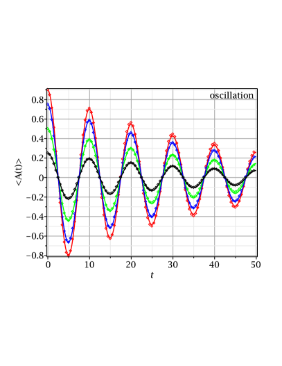
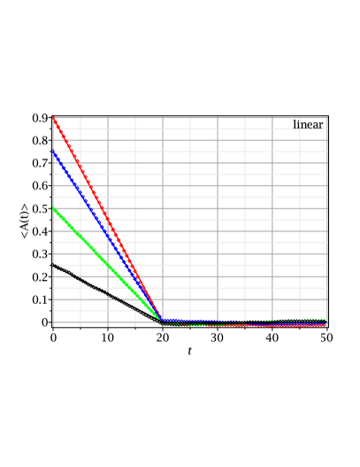
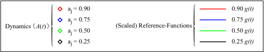
Figure 1: We implemented four pairs of Hamiltonian $H$ and observable $A$ in accord with the ETH ansatz. These implementations are constrained to render $\langle A(t)A\rangle\propto g(t)$ (see Tbl. LABEL:ref_functions for the different $g(t)$). We calculated the expectation value $\bra{j}A(t)\ket{j}$ for four different eigenstates $\ket{j}$ of $A$ (diamonds). The dynamics of $\bra{j}A(t)\ket{j}$ are in good accordance with the scaled reference-functions (curves).

Appendix B Proof of the main Theorem

In this section we proof (5).

B.1 Discretization of (1)

As a first step we rewrite (1) in a time-discrete form. Since the time-step $T=t/N$ is infinitesimal small, we neglect terms of the order $\mathcal{O}(T^{2})$.

$$\rho_{n}=(1-\gamma T)U\rho_{n-1}U^{\dagger}+\gamma T\hat{P}U\rho_{n-1}U^{\dagger}+\mathcal{O}(T^{2})$$ (15)

$U$ denotes the propagator of the closed system for the time-step $T$. $\hat{P}$ is a super-operator that removes all non-diagonal elements in the Basis $\mathfrak{B}$. $\rho_{n}$ denotes the density matrix at the time $t=nT$.

B.2 A recursive model to calculate the expectation value in the decohered system

We now consider the expectation value of $A$:

$$\langle A\rangle_{\rho_{n}}=(1-\gamma T)\tr(AU\rho_{n-1}U^{\dagger})+\gamma T\tr(AU\hat{P}\rho_{n-1}U^{\dagger})$$ (16)

We define $z_{n}(\epsilon)$ recursively:

$$z_{0}(\epsilon)= \langle A\rangle_{\rho_{0}}g(\epsilon)$$ (17)

$$z_{n}(\epsilon)= (1-\gamma T)z_{n-1}(\epsilon+T)+\gamma Tz_{n-1}(0)g(\epsilon+T)$$

In order to show that

$$\langle A\rangle_{\rho_{n}}=z_{n}(0)$$ (18)

is valid, we prove the following equation by induction (over $n$):

$$\tr(AU^{m}\rho_{n}(U^{\dagger})^{m})=z_{n}(mT);m,n\in\mathbb{N}$$ (19)

The base-case ($n=0$) directly follows from (2), since the initial state $\rho_{0}$ is diagonal by definition:

$$\tr(AU^{m}\rho_{0}(U^{\dagger})^{m})=\langle A(mT)\rangle_{\rho_{0}}=\langle A\rangle_{\rho_{0}}g(mT)=z_{0}(mT)$$ (20)

We now prove that, if (19) holds for all $n\in\{0,1,...,k-1\}$ with $k\in\mathbb{N}$, it holds for $n=k$, as well.

$$\tr(AU^{m}\rho_{k}(U^{\dagger})^{m})$$ (21)

$$= (1-\gamma T)\tr(AU^{m+1}\rho_{k-1}(U^{\dagger})^{m+1})$$

$$+ \gamma T\tr(AU^{m+1}\hat{P}\rho_{k-1}(U^{\dagger})^{m+1})$$

We applied the the discrete form of the Lindblad-equation (15). The first summand in this equation can be simplified by applying the induction-assumption (19). Since $\hat{P}\rho_{k-1}$ exhibits diagonal-form regarding $\mathfrak{B}$ we use (2) to simplify the second summand. After applying the induction-assumption (19), we finally find:

$$\tr(AU^{m}\rho_{k}(U^{\dagger})^{m})$$ (22)

$$= (1-\gamma T)z_{k-1}((m+1)T)+\gamma Tz_{k-1}(0)g((m+1)T)$$

B.3 Transforming the recursive model into a partial differential equation

Since the time-step $T$ is infinitesimal, we now transform the recursive definition of $z_{n}$ into a partial differential equation (pde). Therefore we define $z(t=nT,\epsilon)=z_{n}(\epsilon)$ and rewrite (17):

$$z(t,\epsilon) =(1-\gamma T)z(t-T,\epsilon+T)$$ (23)

$$+\gamma Tz(t-T,0)g(\epsilon+T)$$

We linearly approximate $z$ for small $T$ and find:

$$\frac{1}{g(\epsilon)}\left(\gamma z(t,\epsilon)+\frac{\partial z}{\partial{t}}-\frac{\partial z}{\partial\epsilon}\right)=\gamma z(t,0)$$ (24)

For infinitesimal small $T$ this approximation and (23) become equivalent.

The function $z(t,\epsilon)$, that solves this equation and satisfies the boundary condition (17), reads:

$$z(t,\epsilon) =a(\epsilon+t)\exp(-\gamma t)$$ (25)

$$+\int_{0}^{t}\gamma z(t^{\prime},0)g(t+\epsilon-t^{\prime})\exp(-\gamma(t-t^{\prime}))\mathrm{d}t^{\prime}$$

This can be verified by inserting $z(t,\epsilon)$ into (24).

Since we are only interested in the dynamics $\tilde{a}(t)=z(t,0)$, we set $\epsilon=0$:

$$\tilde{a}(t) =a(t)\exp(-\gamma t)$$ (26)

$$+\gamma\int_{0}^{t}\tilde{a}(t^{\prime})g(t-t^{\prime})\exp(-\gamma(t-t^{\prime}))\mathrm{d}t^{\prime}$$

B.4 Expressing the solution in terms of Memory-Kernels

In this section we use the laplace-transform to rewrite the result (26) in terms of memory-kernels and to prove (5). Therefor we introduce the following laplace-transforms:

$$a(t)\laplace A(s),\tilde{a}(t)\laplace\tilde{A}(s)$$ (27)

$$K(t)\laplace\kappa(s),\tilde{K}(t)\laplace\tilde{\kappa}(s)$$

By transforming (4) for the decoupled case ($\gamma=0$), we find:

$$sA(s)-a_{0}=-\kappa(s)A(s)$$ (28)

$a(0)=\tilde{a}(0)=a_{0}$ follows from (26).

We now prove that the dynamics $\tilde{a}(t)$ of the coupled system (26) is generated by the memory-kernel $\tilde{K}(\tau)$, which is given by our main theorem (5).

The laplace-transform of (5) reads:

$$\tilde{\kappa}(s)=\kappa(s+\gamma)$$ (29)

Firstly we transform (26) and use (28):

$$\tilde{A}(s)= A(s+\gamma)+\gamma\frac{1}{a_{0}}\tilde{A}(s)A(s+\gamma)$$ (30)

$$= (a_{0}+\gamma\tilde{A}(s))\frac{1}{s+\gamma+\kappa(s+\gamma)}$$

$$= (a_{0}+\gamma\tilde{A}(s))\frac{1}{s+\gamma+\tilde{\kappa}(s)}$$

In the last step we used (29).

This equation can be transformed algebraically:

$$s\tilde{A}(s)-a_{0}=-\tilde{\kappa}(s)\tilde{A}(s)$$ (31)

By applying the inverse laplace-transform we finally find:

$$\dot{\tilde{a}}(t)=-\int_{0}^{t}\tilde{K}(t-t^{\prime})\tilde{a}(t^{\prime})\mathrm{d}t^{\prime}$$ (32)

Thus the dynamics $\tilde{a}(t)$ of the coupled system is generated by the memory-kernel, which is given by our main theorem.

References

- Breuer et al. (2002) Heinz-Peter Breuer, Francesco Petruccione, et al., The theory of open quantum systems (Oxford University Press on Demand, 2002).
- Joos et al. (2013) Erich Joos, H Dieter Zeh, Claus Kiefer, Domenico JW Giulini, Joachim Kupsch, and Ion-Olimpiu Stamatescu, Decoherence and the appearance of a classical world in quantum theory (Springer Science & Business Media, 2013).
- Zurek (2003) Wojciech Hubert Zurek, “Decoherence, einselection, and the quantum origins of the classical,” Rev. Mod. Phys. 75, 715–775 (2003).
- Skinner and Hsu (1986) J. L. Skinner and D. Hsu, “Pure dephasing of a two-level system,” The Journal of Physical Chemistry 90, 4931–4938 (1986), https://doi.org/10.1021/j100412a013 .
- Alicki (2004) Robert Alicki, “Pure decoherence in quantum systems,” Open Systems & Information Dynamics 11, 53–61 (2004).
- Esposito and Gaspard (2003) Massimiliano Esposito and Pierre Gaspard, “Spin relaxation in a complex environment,” Phys. Rev. E 68, 066113 (2003).
- Deutsch (1991) J. M. Deutsch, “Quantum statistical mechanics in a closed system,” Phys. Rev. A 43, 2046–2049 (1991).
- Srednicki (1999) Mark Srednicki, “The approach to thermal equilibrium in quantized chaotic systems,” Journal of Physics A: Mathematical and General 32, 1163 (1999).
- Rigol et al. (2008) Marcos Rigol, Vanja Dunjko, and Maxim Olshanii, “Thermalization and its mechanism for generic isolated quantum systems,” Nature 452, 854 EP – (2008).
- D’Alessio et al. (2016) L. D’Alessio, Y. Kafri, A. Polkovnikov, and M. Rigol, “From quantum chaos and eigenstate thermalization to statistical mechanics and thermodynamics,” Advances in Physics 65, 239–362 (2016), arXiv:1509.06411 [cond-mat.stat-mech] .
- Beugeling et al. (2015) Wouter Beugeling, Roderich Moessner, and Masudul Haque, “Off-diagonal matrix elements of local operators in many-body quantum systems,” Phys. Rev. E 91, 012144 (2015).
- Mondaini and Rigol (2017) Rubem Mondaini and Marcos Rigol, “Eigenstate thermalization in the two-dimensional transverse field ising model. ii. off-diagonal matrix elements of observables,” Phys. Rev. E 96, 012157 (2017).
- Richter et al. (2018) J. Richter, J. Gemmer, and R. Steinigeweg, “Impact of Eigenstate Thermalization on the Route to Equilibrium,” ArXiv e-prints (2018), arXiv:1805.11625 [cond-mat.stat-mech] .
- Toda et al. (2012) M. Toda, R. Kubo, R. Kubo, M. Toda, N. Saito, N. Hashitsume, and N. Hashitsume, Statistical Physics II: Nonequilibrium Statistical Mechanics, Springer Series in Solid-State Sciences (Springer Berlin Heidelberg, 2012).
- Esposito and Gaspard (2005) M. Esposito and P. Gaspard, “Emergence of diffusion in finite quantum systems,” Phys. Rev. B 71, 214302 (2005).
- Žnidarič (2010) Marko Žnidarič, “Exact solution for a diffusive nonequilibrium steady state of an open quantum chain,” Journal of Statistical Mechanics: Theory and Experiment 2010, L05002 (2010).
- Žnidarič and Horvat (2013) Marko Žnidarič and Martin Horvat, “Transport in a disordered tight-binding chain with dephasing,” The European Physical Journal B 86, 67 (2013).
- Kassal and Aspuru-Guzik (2012) Ivan Kassal and Alán Aspuru-Guzik, “Environment-assisted quantum transport in ordered systems,” New Journal of Physics 14, 053041 (2012).
- Khatami et al. (2013) Ehsan Khatami, Guido Pupillo, Mark Srednicki, and Marcos Rigol, “Fluctuation-dissipation theorem in an isolated system of quantum dipolar bosons after a quench,” Phys. Rev. Lett. 111, 050403 (2013).
- Gross and Bloch (2017) Christian Gross and Immanuel Bloch, “Quantum simulations with ultracold atoms in optical lattices,” Science 357, 995–1001 (2017), http://science.sciencemag.org/content/357/6355/995.full.pdf .
- Weiss (2012) Ulrich Weiss, Quantum dissipative systems, Vol. 13 (World scientific, 2012).
- Steinigeweg et al. (2017) R. Steinigeweg, F. Jin, H. De Raedt, K. Michielsen, and J. Gemmer, “Charge diffusion in the one-dimensional hubbard model,” Phys. Rev. E 96, 020105 (2017).
- Niemeyer et al. (2014) Hendrik Niemeyer, Kristel Michielsen, Hans De Raedt, and Jochen Gemmer, “Macroscopically deterministic markovian thermalization in finite quantum spin systems,” Phys. Rev. E 89, 012131 (2014).
- Niemeyer et al. (2013) Hendrik Niemeyer, Daniel Schmidtke, and Jochen Gemmer, “Onset of fokker-planck dynamics within a closed finite spin system,” EPL (Europhysics Letters) 101, 10010 (2013).
- Monteoliva and Paz (2000) Diana Monteoliva and Juan Pablo Paz, “Decoherence and the rate of entropy production in chaotic quantum systems,” Phys. Rev. Lett. 85, 3373–3376 (2000).
- Rebentrost et al. (2009) Patrick Rebentrost, Masoud Mohseni, Ivan Kassal, Seth Lloyd, and Alán Aspuru-Guzik, “Environment-assisted quantum transport,” New Journal of Physics 11, 033003 (2009).
- Plenio and Huelga (2008) M B Plenio and S F Huelga, “Dephasing-assisted transport: quantum networks and biomolecules,” New Journal of Physics 10, 113019 (2008).