Generalized Sparse Additive Models

Abstract

We present a unified framework for estimation and analysis of generalized additive models in high dimensions. The framework defines a large class of penalized regression estimators, encompassing many existing methods. An efficient computational algorithm for this class is presented that easily scales to thousands of observations and features. We prove minimax optimal convergence bounds for this class under a weak compatibility condition. In addition, we characterize the rate of convergence when this compatibility condition is not met. Finally, we also show that the optimal penalty parameters for structure and sparsity penalties in our framework are linked, allowing cross-validation to be conducted over only a single tuning parameter. We complement our theoretical results with empirical studies comparing some existing methods within this framework.

1 Introduction

In this paper, we model a response variable as an additive function of a potentially large number of covariates. The problem can be formulated as follows: we are given $n$ observations with response $y_{i}\in\mathbb{R}$ and covariates $\boldsymbol{x}_{i}\in\mathbb{R}^{p}$ for $i=1,\ldots,n$. The goal is to fit the model

$$g\left(\mathbb{E}\left(y_{i}|\boldsymbol{x}_{i}\right)\right)=\beta_{0}+\sum_{j=1}^{p}f_{j}\left(x_{ij}\right),\quad i=1,\ldots,n,$$

for a prespecified link function $g$, unknown intercept $\beta_{0}$ and, unknown component functions $f_{1},\ldots,f_{p}$. The link function, $g$, is generally based on the outcome data-type, e.g., $g(x)=x$ or $g(x)=\log(x)$ for continuous or count response data, respectively. The estimands, $f_{1},\ldots,f_{p}$, give the conditional relationships between each feature $x_{ij}$ and the outcome $y_{i}$ for all $i$ and $j$. For identifiability, we assume $\sum_{i=1}^{n}f_{j}(x_{ij})=0$ for all $j=1,\ldots,p$. This model is known as a generalized additive model (GAM) (Hastie and Tibshirani, 1990). It extends the generalized linear model (GLM) where each $f_{j}$ is linear, and is a popular choice for modeling different types of response variables as a function of covariates. GAMs are popular because they extend GLMs to model non-linear conditional relationships while retaining some interpretability (we can examine the effect of each covariate $x_{ij}$ individually on $y_{i}$ while holding all other variables fixed); they also do not suffer from the curse of dimensionality.

While there are a number of proposals for estimating GAMs, a popular approach is to encode the estimation in the following convex optimization problem (Sadhanala and Tibshirani, 2018):

$$\widehat{\beta},\widehat{f}_{1},\ldots,\widehat{f}_{p}\leftarrow\underset{\beta\in\mathbb{R},f_{1},\ldots,f_{p}\in\mathcal{F}}{\operatorname{argmin}}\ -n^{-1}\sum_{i=1}^{n}\ell\Big{(}y_{i},\beta+\sum_{j=1}^{p}f_{j}\left(x_{ij}\right)\Big{)}+\lambda_{st}\sum_{j=1}^{p}P_{st}\left(f_{j}\right).$$ (1)

Here $\mathcal{F}$ is some suitable function class; $\ell(y_{i},\theta)$ is the log-likelihood of $y_{i}$ under parameter $\theta$; $P_{st}$ is a structure-inducing penalty to control the wildness of the estimated functions, $\widehat{f}_{j}$; and $\lambda_{st}>0$ is a penalty parameter which modulates the trade-off between goodness-of-fit and structure/smoothness of estimates. The class $\mathcal{F}$ is a general convex space, e.g., $\mathcal{F}=L^{2}[0,1]$. Functions $-\ell(y_{i},\theta)$ and $P_{st}(f_{j})$ are convex in $\theta$ and $f_{j}$, respectively. The objective function in (1) is convex and for small dimension, $p$, can be solved via a general-purpose convex solver. However, many modern datasets are high-dimensional, often with more features than observations, i.e., $p>n$. Fitting even GLMs is challenging in such settings as conventional methods are known to overfit the data. A common assumption in the high-dimensional setting is sparsity, that is, only a small (but unknown) subset of features is informative for the outcome. In this case, it is desirable to apply feature selection: to build a model for which only a small subset of $\widehat{f}_{j}\not\equiv 0$.

A number of estimators have been proposed for fitting GAMs with sparsity. These estimators are generally solutions to a convex optimization problem. Though they differ in details, we show that most of these optimization problems can be written as:

$$\small\widehat{\beta},\widehat{f}_{1},\ldots,\widehat{f}_{p}\leftarrow\underset{\beta\in\mathbb{R},f_{1},\ldots,f_{p}\in\mathcal{F}}{\operatorname{argmin}}-n^{-1}\sum_{i=1}^{n}\ell\Big{(}y_{i},\beta+\sum_{j=1}^{p}f_{j}\left(x_{ij}\right)\Big{)}+\lambda_{st}\sum_{j=1}^{p}P_{st}\left(f_{j}\right)+\lambda_{sp}\sum_{j=1}^{p}\left\|f_{j}\right\|_{n},$$ (2)

where $\|f_{j}\|_{n}=\Big{[}n^{-1}\sum_{i=1}^{n}\{f_{j}(x_{ij})\}^{2}\Big{]}^{1/2}$ is a group lasso-type penalty (Yuan and Lin, 2006) for feature-wise sparsity, and $\lambda_{sp}$ a sparsity-related tuning parameter (Ravikumar et al., 2009; Lou et al., 2016; Petersen et al., 2016; Sadhanala and Tibshirani, 2018; Koltchinskii and Yuan, 2010; Raskutti et al., 2012; Yuan and Zhou, 2015; Meier et al., 2009). However, previous proposals consists of gaps around efficient computation (Koltchinskii and Yuan, 2010; Raskutti et al., 2012; Yuan and Zhou, 2015) and/or optimal statistical convergence properties (Ravikumar et al., 2009; Lou et al., 2016; Petersen et al., 2016; Sadhanala and Tibshirani, 2018). General-purpose convex solvers have also been suggested (Koltchinskii and Yuan, 2010; Raskutti et al., 2012; Yuan and Zhou, 2015) as an alternative for solving problem (2), but they roughly scale as $O(n^{3}p^{3})$ and are hence inefficient. This manuscript aims to bridge these gaps.

We present a general framework for sparse GAMs with two major contributions, a general algorithm for computing (2) and a theorem for establishing convergence rates. Briefly, our algorithm is based on accelerated proximal gradient descent. This reduces (2) to repeatedly solving a univariate penalized least squares problem. In many cases, this algorithm has a per-iteration complexity of $O(np)$ — precisely that of state-of-the-art algorithms for the lasso (Friedman et al., 2010; Beck and Teboulle, 2009b). Our main theorem establishes fast convergence rates of the form $\max(s\log p/n,s\xi_{n})$, where $s$ is the number of signal variables and $\xi_{n}$ is the minimax rate of the univariate regression problem, i.e., problem (1) with $p=1$. Nonparametric rates are established for a wide class of structural penalties $P_{st}$ with $\xi_{n}=n^{-2m/(2m+1)}$, popular choices of $P_{st}$ include $m$-th order Sobolev and Hölder norms, total variation norm of the $m$-th derivative and, norms of Reproducing Kernel Hilbert Spaces (RKHS). Parametric rates are also established with $\xi_{n}=T_{n}/n$ via a truncation-penalty; the number of parameters, $T_{n}$, can be fixed or allowed to grow with sample size.

The highlight of this paper is the generality of the proposed framework: not only does it encompass many existing estimators for high-dimensional GAMs, but also estimators for low-dimensional GAMs, low-dimensional fully nonparametric models and, parametric models in low or high-dimensional settings. As a byproduct of our general theorem, we also determine that $\lambda_{st}=\lambda_{sp}^{2}$ in (2) results in optimal convergence rates, reducing the problem to a single tuning parameter.

The rest of the paper is organized as follows. In Section 2, we detail our framework and discuss various choices of structural penalties, $P_{st}$, illustrating that our framework encompasses many existing proposals. In Section 3 we present an algorithm for solving the optimization problem (2) for a broad class of $P_{st}$ penalties, and establish their theoretical convergence rates in Section 4. We explore the empirical performance of various choices of $P_{st}$ in simulation in Section 5, and in an application to the Boston housing dataset in Section 6. Concluding remarks are in Section 7.

2 General Framework for Additive Models

In this section, we present our general framework for estimating sparse GAMs, discuss its salient features, and review some existing methods as special cases. Before presenting our framework, we introduce some notation. For any function $f$ and response/covariate pair, $(y,\boldsymbol{x})$, let $-\ell(f)\equiv-\ell(y,f({\boldsymbol{x}}))$ denote a loss function; given data $(y_{1},\boldsymbol{x}_{1}),\ldots,(y_{n},\boldsymbol{x}_{n})$, let $\mathbb{P}_{n}\ell(f)\equiv n^{-1}\sum_{i=1}^{n}\ell(y_{i},f({\boldsymbol{x}}_{i}))$ denote an empirical average; and $\|f\|_{n}^{2}\equiv n^{-1}\sum_{i=1}^{n}f({\boldsymbol{x}}_{i})^{2}$ denote the empirical norm. With some abuse of notation, we will use the shorthand $f_{j}$ to denote the function $f_{j}\circ\pi_{j}$ where $\pi_{j}(\boldsymbol{x})=x_{j}$ for $\boldsymbol{x}\in\mathbb{R}^{p}$.

Our general framework for obtaining a Generalized Sparse Additive Model (GSAM) encompasses estimators that can be obtained by solving the following problem:

$$\widehat{\beta},\widehat{f}_{1},\ldots,\widehat{f}_{p}\leftarrow\underset{\beta\in\mathbb{R},f_{1},\ldots,f_{p}\in\mathcal{F}}{\operatorname{argmin}}\underbrace{-\mathbb{P}_{n}\ell\left(\beta+\sum_{j=1}^{p}f_{j}\right)}_{\text{Goodness-of-fit}}+\underbrace{\lambda^{2}\sum_{j=1}^{p}P_{st}\left(f_{j}\right)}_{\text{structure-inducing}}+\underbrace{\lambda\sum_{j=1}^{p}\left\|f_{j}\right\|_{n}}_{\text{sparsity-inducing}}.$$ (3)

This optimization problem balances three terms. The first is a loss function based on goodness-of-fit to the observed data; the least squares loss, $-\ell(f)=(y-f(\boldsymbol{x}))^{2}$, is commonly used for continuous response. Our general framework requires only convexity and differentiability of $-\ell(y,\theta)$, with respect to $\theta$. Later we consider loss functions given by the negative log-likelihood of exponential family distributions. The second piece is a penalty to induce smoothness/structure of the function estimates. Our framework requires $P_{st}$ to be a semi-norm on $\mathcal{F}$. This choice is motivated by both statistical theory and computational efficiency; we discuss this along with possible choices of $P_{st}$ in the following sub-sections. The final piece is a sparsity penalty $\|\cdot\|_{n}$, which encourages models with $\widehat{f}_{j}\equiv 0$ for many $j$. Surprisingly, $P_{st}$ also plays an important role in obtaining an appropriate sparsity pattern. Briefly, if $P_{st}$ is a squared semi-norm then either all $\widehat{f}_{j}\equiv 0$ or all $\widehat{f}_{j}\not\equiv 0$. To fit models where some $\widehat{f}_{j}\equiv 0$ and not others, the non-differentiablity of semi-norms at 0 is crucial, we detail this in Section 2.2 below. Throughout this manuscript, we require the function class $\mathcal{F}$ to be a convex cone, e.g., $L^{2}(\mathbb{R})$. Later for some specific results, we will additionally require $\mathcal{F}$ to be a linear space.

As noted before, the tuning parameters for structure ($\lambda$) and sparsity ($\lambda^{2}$) are coupled in our framework. The theoretical consequence of this is that, for properly chosen $\lambda$, we get rate-optimal estimates (shown in Section 4). The practical consequence is that we have a single tuning parameter. This is adequate for most choices of $P_{st}$ as seen in our empirical experiments of Section 5.

Furthermore, our framework relaxes the usual distributional requirements of i.i.d. response from an exponential family; we require only $y_{i}$ independent and $E\{y_{i}-E(y_{i})\}$ to be sub-Gaussian (or sub-Exponential). This demonstrates the generality of our framework and highlights our main innovation: the efficient algorithm of Section 3 and theoretical results of Section 4 apply to a very broad class of estimators, fill in the gaps of existing work and, can easily be applied for the development of future estimators.

2.1 Structure Inducing Penalties

We now present some possible choices of the structural penalty $P_{st}$ followed by a discussion of the conditions on $P_{st}$ that lead to desirable estimation and computation. The main requirement is that $P_{st}$ is a semi-norm: a functional that obeys all the rules of a norm except one — for nonzero $f$ we may have $P_{st}(f)=0$. Some potential choices for smoothing semi-norms are:

1. $k$-th order Sobolev $P_{st}\leftarrow P_{sobolev}(f^{(k)})=\sqrt{\int_{x}\left\{f^{(k)}(x)\right\}^{2}dx}$;

2. $k$-th order total variation $P_{st}\leftarrow{TV}(f^{(k)})$;

3. $k$-th order Hölder $P_{st}\leftarrow P_{holder}(f^{(k)})=\operatorname{sup}_{x}\left|f^{(k)}(x)\right|$;

4. $k$-th order monotonicity $P_{st}\leftarrow P_{mon}(f^{(k)})\leftarrow\mathbb{I}\left(f;\ \{f:f^{(k+1)}\geq 0\}\right)$;

5. $M$-th dimensional linear subspace $P_{st}\leftarrow P^{M}_{lin}(f)=\mathbb{I}\left(f;\ \textrm{span}\left\{g_{1},\ldots,g_{M}\right\}\right)$;

here $TV(\cdot)$ is the total variation norm, $TV(f)=\sup\{\sum_{i=1}^{o}|f(z_{i+1})-f(z_{i})|:z_{1}<\ldots<z_{o}\text{ is a partition of }[0,1]\}$, and $\mathbb{I}$ is a convex indicator function defined as $\mathbb{I}(f;\mathcal{A})=0$ if $f\in\mathcal{A}$ and $\mathbb{I}(f;\mathcal{A})=\infty$ if $f\not\in\mathcal{A}$. As implied by the name, $P_{st}$ imposes smoothness or structure on individual components $\widehat{f}_{j}$. For instance, $P_{sobolev}(f^{\prime\prime})$ is a common measure of smoothness; small $\lambda$ values leads to wiggly fitted functions $\widehat{f}_{j}$; on the other hand, sufficiently large $\lambda$ values would lead to each component being a linear function. The convex indicator function, $\mathbb{I}(\cdot)$, can impose specific structural properties on $\widehat{f}_{j}$; e.g., $P_{mon}(f)$ fits a model with each $\widehat{f}_{j}$ a non-decreasing function.

The semi-norm requirement for $P_{st}$ is important because: (a) it implies convexity leading to a convex objective function, (b) the first order absolute homogeneity ($P_{st}(\alpha f)=|\alpha|P_{st}(f)$) is needed for the algorithm of Section 3 and, (c) the triangle inequality is used throughout the proof of our theoretical results of Section 4. For our context, we consider convex indicators of cones as a semi-norm because, the first order homogeneity condition can be relaxed. For our algorithm, we only require $P_{st}(\alpha f)=\alpha P_{st}(f)$ for $\alpha>0$; for our theoretical results we treat convex indicators of cones as a special case and discuss them at the end of Section 4.2. For non-sparse GAMs of the form (1), the existing literature does not necessarily use a semi-norm penalty; a common choice of smoothing penalty is $P_{st}(f)=P^{2}_{sobolev}(f^{\prime\prime})$. In the following subsection, we discuss the issues with using squared semi-norm penalties in high dimensions, particularly their impact on the sparsity of estimated component functions.

2.2 Semi-norms vs Squared Semi-norms

Given a semi-norm $P_{semi}$, using $P_{st}=P_{semi}^{2}$ in (3) may give poor theoretical performance (as noted in Meier et al. (2009) for $P_{semi}=P_{sobolev}$) and, can also be computationally expensive (as disscussed in Section 3). In this subsection, we show a surprising result: using a squared semi-norm penalty does not actually lead to a sparse solution.

To be precise, using $P_{st}=P_{semi}^{2}$ leads to an active set ${S}=\{j:\widehat{f}_{j}\not\equiv 0\}$, for which either $|{S}|=0$ or $|{S}|=p$; in contrast, using $P_{st}=P_{semi}$ can give active sets such that $0<|{S}|<p$. To demonstrate this phenomenon, we consider first the univariate problem

$$\widehat{f}_{1}\leftarrow\underset{f\in\mathcal{F}}{\operatorname{argmin}}\ \frac{1}{n}\sum_{i=1}^{n}\left(y_{i}-f\left(x_{i}\right)\right)^{2}+\lambda_{st}P^{2}_{semi}\left(f\right)+\lambda_{sp}\left\|f\right\|_{n},$$ (4)

and characterize conditions for which $\widehat{f}_{1}\equiv 0$. Recall that $\widehat{f}_{1}$ minimizes the objective in (4) if for every direction $h$, the objective is minimized at $\varepsilon=0$ along the path $\widehat{f}_{1}+\varepsilon h$. The following lemma gives necessary and sufficient conditions for $\widehat{f}_{1}$ to be $\boldsymbol{0}$.

Lemma 1.

For $\widehat{f}_{1}$ given by (4), the following are equivalent: (a) $\widehat{f}_{1}=\boldsymbol{0}$, (b) for every direction $h\in\mathcal{F}$, $\left|{n^{-1}}\sum_{i}y_{i}{h(x_{i})}/{\left\|h\right\|_{n}}\right|\leq\lambda_{sp}$, (c) $\|\boldsymbol{y}\|_{n}\leq\lambda_{sp}$.

Lemma 1 is proved in Appendix LABEL:sec:ProofSec2 in the supplementary material. Condition (c) of Lemma 1 is problematic when we consider multiple features in our additive problem (3). For additive models, condition (c) implies that sparsity of component $\widehat{f}_{j}$, does not depend on covariate $j$. Thus if all smoothing penalties are squared semi-norms then for a given $\lambda_{sp}$, there exists a minimizer with either all $\widehat{f}_{j}={\bf 0}$ or all $\widehat{f}_{j}\not={\bf 0}$. Consider, instead, the optimization problem

$$\widehat{f}_{2}\leftarrow\underset{f\in\mathcal{F}}{\operatorname{argmin}}\ \frac{1}{n}\sum_{i=1}^{n}\left(y_{i}-f\left(x_{i}\right)\right)^{2}+\lambda_{st}P_{semi}\left(f\right)+\lambda_{sp}\left\|f\right\|_{n}.$$ (5)

For this problem, we obtain the following result (proof in Appendix LABEL:sec:ProofSec2 in the supplementary material).

Lemma 2.

For $\widehat{f}_{2}$ defined by (5), the following are equivalent: (a) $\widehat{f}_{2}=\boldsymbol{0}$, (b) for every direction $h$, there exists some $V\in[-1,1]$ such that $\Big{|}{n^{-1}}\sum_{i}y_{i}{h(x_{i})}/{\|h\|_{n}}-\lambda_{st}{VP_{semi}(h)}/{\|h\|_{n}}\Big{|}\leq\lambda_{sp}$. Additionally, if $\|\boldsymbol{y}\|_{n}\leq\lambda$ then $\widehat{f}_{2}=\boldsymbol{0}$, but the converse is not necessarily true.

Unlike the squared semi-norm penalties, conditions for $\widehat{f}_{2}=\boldsymbol{0}$ involve the feature vector $\boldsymbol{x}$. Thus for an additive model the sparsity of component $j$ depends on both the response vector $\boldsymbol{y}$, and $j$-th covariate $(x_{1j},\ldots,x_{nj})$. Consequently, there are many $(\lambda_{sp},\lambda_{st})$ pairs for which we will have some $\widehat{f}_{j}={\bf 0}$ and some $\widehat{f}_{j}\not={\bf 0}$. Additionally, Lemma 2 gives us a conservative value for $\lambda_{max}=\|\boldsymbol{y}\|_{n}$, i.e., the $\lambda_{sp}$ value for which all $\widehat{f}_{j}=\boldsymbol{0}$.

2.3 Relationship of Existing Methods to GSAM

We now discuss some of the existing methods for sparse additive models in greater detail, and demonstrate that many existing proposals are special cases of our GSAM framework. One of the first proposals for sparse additive models, SpAM (Ravikumar et al., 2009), uses a basis expansion and solves

$$\underset{\beta_{1},\ldots,\beta_{j}\in\mathbb{R}^{M}}{\operatorname{argmin}}\ \Big{\|}{\boldsymbol{y}}-\sum_{j=1}^{p}\sum_{m=1}^{M}\beta_{jm}\boldsymbol{\psi}_{jm}\Big{\|}_{n}^{2}+\lambda\sum_{j=1}^{p}\Big{\|}\sum_{m=1}^{M}\beta_{jm}\boldsymbol{\psi}_{jm}\Big{\|}_{n},$$ (6)

where $\boldsymbol{\psi}_{jm}=[\psi_{m}(x_{1j}),\ldots,\psi_{m}(x_{nj})]^{T}\in\mathbb{R}^{n}$ for basis functions $\psi_{1},\ldots,\psi_{M}$. This is a GSAM with $P_{st}=\mathbb{I}\left(f;\textrm{span}\left\{\psi_{1},\ldots,\psi_{M}\right\}\right)$. The SpAM proposal is extended to partially linear models in SPLAM (Lou et al., 2016). There, a similar basis expansion is used, though with the particular choice $\psi_{1}(x)=x$. The SPLAM estimator solves

$$\small\underset{\beta_{1},\ldots,\beta_{j}\in\mathbb{R}^{M}}{\operatorname{argmin}}\ \Big{\|}{\boldsymbol{y}}-\sum_{j=1}^{p}\sum_{m=1}^{M}\beta_{jm}\boldsymbol{\psi}_{jm}\Big{\|}_{n}^{2}+\lambda_{1}\sum_{j=1}^{p}\Big{\|}\sum_{m=1}^{M}\beta_{jm}\boldsymbol{\psi}_{jm}\Big{\|}_{n}+\lambda_{2}\sum_{j=1}^{p}\Big{\|}\sum_{m=2}^{M}\beta_{jm}\boldsymbol{\psi}_{m}\Big{\|}_{n},$$ (7)

and is also a GSAM with

$$P_{st}=\mathbb{I}\left(f;\textrm{span}\left\{\psi_{1},\ldots,\psi_{M}\right\}\right)+\sum_{j=1}^{p}\Big{\|}\operatorname{Proj}_{\operatorname{span}\left(\psi_{2},\ldots,\psi_{M}\right)}\left(f\right)\Big{\|}_{n},$$

where $\operatorname{Proj}_{A}$ is the projection operator onto the set $A$. The recently proposed extensions of trend filtering to additive models are other examples (Petersen et al., 2016; Sadhanala and Tibshirani, 2018); these methods can be written in our GSAM framework with $P_{st}(f)=TV(f)$.

Koltchinskii and Yuan (2010), Raskutti et al. (2012) and Yuan and Zhou (2015) discuss a similar framework to GSAMs; however, they only consider structural penalties $P_{st}$, which are norms of Reproducing Kernel Hilbert Spaces (RKHS). Furthermore, they do not discuss efficient algorithms for solving the convex optimization problem. Using properties of RKHS, they note that their estimator is the minimum of a $d=np$ dimensional second order cone program (SOCP). The computation for general-purpose SOCP solvers scales roughly as $d^{3}$. Thus for even moderate $p$ and $n$, these problems quickly become intractable.

Meier et al. (2009) give two proposals: the first solves the optimization problem

$$\underset{f_{1},\ldots,f_{p}\in\mathcal{F}}{\operatorname{argmin}}\ \Big{\|}\boldsymbol{y}-\sum_{j=1}^{p}f_{j}\Big{\|}_{n}^{2}+\sum_{j=1}^{p}\lambda_{sp}\sqrt{\left\|f_{j}\right\|^{2}_{n}+\lambda_{st}P_{st}^{2}\left(f_{j}\right)},$$

and is not a GSAM; they note that this proposal gives a suboptimal rate of convergence. The second is a GSAM of the form (3) with $P_{st}(f)=P_{sobolev}(f^{\prime\prime})$. At the time, Meier et al. (2009) focused on the first proposal as no computationally efficient method for solving the second one was known to them. In a follow-up paper, van de Geer (2010) studied the theoretical properties of a GSAM with an alternative, diagonalized smoothness structural penalty. The diagnolized smoothness penalty for a function with basis expansion $f_{\boldsymbol{\beta}}(x)=\sum_{j=1}^{n}\psi_{j}(x)\beta_{j}$, is defined as

$$P_{st}(f_{\boldsymbol{\beta}})=\Big{(}{\sum_{j=1}^{n}j^{2m}\beta_{j}^{2}}\Big{)}^{1/2},$$ (8)

for a smoothness parameter $m$. All of the above mentioned proposals either fail to provide an efficient computational algorithm or have sub-optimal convergence rates. There are also a number of other proposals that do not quite fall in the GSAM framework (Chouldechova and Hastie, 2015; Fan et al., 2012; Yin et al., 2012).

3 General-Purpose Algorithm

Here we give a general algorithm for fitting GSAMs based on proximal gradient descent (Parikh and Boyd, 2014). We begin with some notation. We denote by $\dot{\ell}(y,\theta)$ and $\ddot{\ell}(y,\theta)$ the first and second derivatives of $\ell$ with respect to $\theta$. For functions $f,g:\mathbb{R}^{p}\to\mathbb{R}$, let $\langle f,\dot{\ell}(g)\rangle_{n}\equiv{n^{-1}}\sum_{i=1}^{n}f(\boldsymbol{x}_{i})\{\dot{\ell}(y_{i},g(\boldsymbol{x}_{i}))\}$, $\mathbb{P}_{n}{\dot{\ell}}(g)\equiv{n^{-1}}\sum_{i=1}^{n}\dot{\ell}(y_{i},g(\boldsymbol{x}_{i}))$ and, $\|f+\dot{\ell}(g)\|_{n}^{2}\equiv{n^{-1}}\sum_{i=1}^{n}\{f(\boldsymbol{x}_{i})+\dot{\ell}(y_{i},g(\boldsymbol{x}_{i}))\}^{2}$.

We begin with a second order Taylor expansion of the loss. For this, we first apply Taylor’s theorem to $\ell(y_{i},\beta+\theta_{i1}+\ldots+\theta_{ip})$ as a $(p+1)$ variate function of $(\beta,\theta_{i1},\ldots,\theta_{ip})$. Note that for $|\ddot{\ell}(y,\theta)|\leq L$, the Hessian matrix, $H_{p+1}$, of $\ell(y_{i},\beta+\theta_{i1}+\ldots+\theta_{ip})$ obeys the inequality $\boldsymbol{a}^{T}H_{p+1}\boldsymbol{a}\leq(p+1)L\|a\|_{2}^{2}$ for all $\boldsymbol{a}\in\mathbb{R}^{p+1}$ (Zhan, 2005). This gives us the following bound:

$$-\mathbb{P}_{n}\ell\Big{(}\beta+\sum_{j=1}^{p}f_{j}\Big{)} \leq-\mathbb{P}_{n}\ell\Big{(}\beta^{0}+\sum_{j=1}^{p}f^{0}_{j}\Big{)}$$

$$-(\beta-\beta^{0})\mathbb{P}_{n}\dot{\ell}\Big{(}\beta^{0}+\sum_{j=1}^{p}f^{0}_{j}\Big{)}-\sum_{j=1}^{p}\Big{\langle}f_{j}-f^{0}_{j},\dot{\ell}\Big{(}\beta^{0}+\sum_{j=1}^{p}f^{0}_{j}\Big{)}\Big{\rangle}_{n}$$

$$+\frac{(p+1)L}{2}(\beta-\beta^{0})^{2}+\sum_{j=1}^{p}\frac{(p+1)L}{2}\left\|f_{j}-f^{0}_{j}\right\|_{n}^{2},$$

which leads to the following majorizing inequality

$$\begin{split}-\mathbb{P}_{n}\ell\Big{(}\beta+\sum_{j=1}^{p}f_{j}\Big{)}&\leq\frac{(p+1)L}{2}\Big{[}\beta-\Big{\{}\beta^{0}+\frac{1}{(p+1)L}\mathbb{P}_{n}\dot{\ell}\Big{(}\beta^{0}+\sum_{j=1}^{p}f^{0}_{j}\Big{)}\Big{\}}\Big{]}^{2}\\ &+\sum_{j=1}^{p}\frac{(p+1)L}{2}\Big{\|}f_{j}-\Big{\{}f^{0}_{j}+\frac{1}{(p+1)L}\dot{\ell}\Big{(}\beta^{0}+\sum_{j=1}^{p}f^{0}_{j}\Big{)}\Big{\}}\Big{\|}_{n}^{2}+W,\end{split}$$ (9)

where $W$ is not a function of $\beta$ or $f_{j}$ for any $j$. Instead of minimizing the original problem (3), we minimize the majorizing surrogate

$$\frac{1}{2}\Big{[}\beta-\Big{\{}\beta^{0}+{t}\mathbb{P}_{n}\dot{\ell}\Big{(}\beta^{0}+\sum_{j=1}^{p}f^{0}_{j}\Big{)}\Big{\}}\Big{]}^{2} +\frac{1}{2}\sum_{j=1}^{p}\Big{\|}f_{j}-\Big{\{}f^{0}_{j}+{t}\dot{\ell}\Big{(}\beta^{0}+\sum_{j=1}^{p}f^{0}_{j}\Big{)}\Big{\}}\Big{\|}_{n}^{2}$$

$$+{t\lambda^{2}}\sum_{j=1}^{p}P_{st}\left(f_{j}\right)+{t\lambda}\sum_{j=1}^{p}\left\|f_{j}\right\|_{n},$$ (10)

where $t=\{(p+1)L\}^{-1}$. Minimizing (3) and re-centering our Taylor series at the current iterate, is precisely the proximal gradient recipe. Updating the intercept $\beta$, is simply $\widehat{\beta}\leftarrow\beta^{0}+t\mathbb{P}_{n}\dot{\ell}\Big{(}\beta^{0}+\sum_{j=1}^{p}f^{0}_{j}\Big{)}$. Components $f_{1},\ldots,f_{p}$, can be updated in parallel by solving the univariate problems:

$$\widehat{f}_{j}\leftarrow\underset{f\in\mathcal{F}}{\operatorname{argmin}}\ \frac{1}{2}\Big{\|}\Big{\{}f^{0}_{j}+t\dot{\ell}\Big{(}\beta^{0}+\sum_{j=1}^{p}f^{0}_{j}\Big{)}\Big{\}}-f\Big{\|}_{n}^{2}+t{\lambda^{2}}P_{st}\left(f\right)+t{\lambda}\left\|f\right\|_{n}.$$ (11)

At first, this problem still appears difficult due to the combination of structure and sparsity penalties. However, the following Lemma shows that things greatly simplify.

Lemma 3.

Suppose $P_{st}$ is a semi-norm, and $\boldsymbol{r}$ is an $n$-vector. Consider the optimization problems

$$\underset{f\in\mathcal{F}}{\operatorname{argmin}}\ \frac{1}{2}\|\boldsymbol{r}-f\|_{n}^{2}+\lambda_{1}P_{st}\left(f\right)+\lambda_{2}\|f\|_{n},$$ (12)

$$\underset{f\in\mathcal{F}}{\operatorname{argmin}}\ \frac{1}{2}\|\boldsymbol{r}-f\|_{n}^{2}+\lambda_{1}P_{st}\left(f\right).$$ (13)

If $\widetilde{f}$ is a solution to (13); then $\widehat{f}$ is a solution to (12) where $\widehat{f}$ is defined as

$$\widehat{f}=\Big{(}1-{\lambda_{2}}/{\|\widetilde{f}\|_{n}}\Big{)}_{+}\widetilde{f},$$ (14)

with $(z)_{+}=\max(z,0)$.

The proof is given in Appendix LABEL:sec:appendix in the supplementary material. Using Lemma 3, we can get the solution to (11) by solving a problem in the form of (13), a classical univariate smoothing problem, and then applying (14), the simple soft-scaling operator. Putting things together, our proximal gradient algorithm for solving (3) is summarized in Algorithm 1.

Algorithm 1 General Proximal Gradient Algorithm for (3)

1:Initialize $f^{0}_{1},\ldots f^{0}_{p}\leftarrow{\bf 0},\beta^{0}\leftarrow 0$, $k\leftarrow 1$; choose a step-size $t$

2:while $k\leq max\_iter$ and not converged do

3:     For each $i=1,\ldots,n$, set

$$\theta_{i}\leftarrow\beta^{k-1}+\sum_{j=1}^{p}f^{k-1}_{j}\left(x_{ij}\right),\quad\quad r_{i}\leftarrow-\dot{\ell}\left(y_{i},\theta_{i}\right).$$

4:     Update $\beta^{k}\leftarrow\beta^{k-1}-t\sum_{i=1}^{n}r_{i}.$

5:     for $j=1,\,\ldots,\,p$ do

6:         Set

$$f^{inter}_{j}\leftarrow\underset{f\in\mathcal{F}}{\operatorname{argmin}}\frac{1}{2}\left\|\left(f_{j}^{k-1}-t\boldsymbol{r}\right)-f\right\|_{n}^{2}+t\lambda^{2}P_{st}\left(f\right).$$ (15)

7:         Update

$$f^{k}_{j}\leftarrow\Big{(}1-{t\lambda}/{\|f^{inter}_{j}\|_{n}}\Big{)}_{+}f^{inter}_{j}.$$

8:     end for

9:end while

10:return $\beta^{k},f^{k}_{1},\ldots,f^{k}_{p}$

Algorithm 1 is simple and can be quite fast: the time complexity is largely determined by the difficulty of solving the univariate smoothing problem of step $5$. In many cases this takes $O(n)$ operations, allowing an iteration of proximal gradient descent to run in $O(np)$ operations. Complexity order $O(np)$ is the per-iteration time complexity of state-of-the-art algorithms for the lasso (Friedman et al., 2010; Beck and Teboulle, 2009a).

Any step-size $t$ can be used in Algorithm 1 so long as inequality (9) holds for $f_{j}^{0}\equiv f_{j}^{k-1}$ and $f_{j}\equiv f_{j}^{k}$ when $(p+1)L$ is replaced by $t^{-1}$. Note that if $t\leq\{L(p+1)\}^{-1}$ this will always hold. However, often $p^{k}_{active}$, the number of $j$ for which either of $f^{k-1}_{j}$ or $f^{k}_{j}$ is non-zero, will be small. In this case $t\leq\{L(p_{active}+1)\}^{-1}$ will satisfy the majorization condition. Since, in practice, we are interested in sparse models, generally $p^{k}_{active}\ll p$ and adaptive step-size optimization can be quite useful (Beck and Teboulle, 2009b) . The algorithm can also take advantage of Nesterov-style acceleration (Nesterov, 2007), which improves the worst-case convergence rate after $k$ steps from $O\left({k}^{-1}\right)$ to $O\left({k^{-2}}\right)$.

An important special case is the least squares loss $-\ell(y,\theta)=(y-\theta)^{2}$. In this case, we can use a block coordinate descent algorithm which can be more efficient than Algorithm 1, and does not require a step-size calculation. We present the full details of the algorithm in Appendix LABEL:app:AdditionalFigures in the supplementary material.

As noted above, the main computational hurdle in Algorithm 1 is solving the univariate problem (13). In the following subsection, we discuss this step in greater detail for various smoothness penalties.

3.1 Solving the Univariate Sub-problem

For many semi-norm smoothers there are already efficient solvers for solving (13): with the $k$-th order total variation penalty, (13) can be solved exactly in $2n$ operations for $k=0$ (Johnson, 2013), or iteratively in roughly $O((k+1)n)$ operations for $k\geq 1$ (Ramdas and Tibshirani, 2015); with the convex indicator of an $M$-dimensional linear subspace, (13) can be solved in $O(M^{2}n)$ operations using linear regression; using a monotonicity indicator, (13) can be solved with the pool adjacent violators algorithm in $O(n)$ operations (Ayer et al., 1955).

For many other choices of $P_{st}$, we do not have efficient algorithms for solving (13); however, we might have fast algorithms for the slightly different optimization problem:

$$\widetilde{f}_{\widetilde{\lambda}}\leftarrow\underset{f\in\mathcal{F}}{\operatorname{argmin}}\ \frac{1}{2}\left\|\boldsymbol{r}-f\right\|_{n}^{2}+\widetilde{\lambda}P_{st}^{\tau}\left(f\right),$$ (16)

for $\tau>1$. For example, the $k$-th order Sobolev penalty (Wahba, 1990) can be solved exactly in $O(kn)$ operations for $\tau=2$. In the following Lemma, we show that the solution to (16) can be leveraged to solve the harder problem (13).

Lemma 4.

Given an $n$-vector $\boldsymbol{r}$, a convex linear space $\mathcal{F}$ over the field $\mathbb{R}$, and real $\tau>1$, consider the optimization problems:

$$\widehat{f}_{\lambda} \leftarrow\underset{f\in\mathcal{F}}{\operatorname{argmin}}\ \frac{1}{2}\left\|\boldsymbol{r}-f\right\|_{n}^{2}+\lambda P_{st}\left(f\right);$$

$$\widetilde{f}_{\lambda} \leftarrow\underset{f\in\mathcal{F}}{\operatorname{argmin}}\ \frac{1}{2}\left\|\boldsymbol{r}-f\right\|_{n}^{2}+\lambda P_{st}^{\tau}\left(f\right);$$

$$f_{null} \leftarrow\underset{f\in\mathcal{F}}{\operatorname{argmin}}\ \frac{1}{2}\left\|\boldsymbol{r}-f\right\|_{n}^{2}+\mathbb{I}\left(f\in\mathcal{F}:P_{st}(f)=0\right);$$

$$f_{interp} \leftarrow\underset{f\in\mathcal{F}}{\operatorname{argmin}}\ P_{st}^{\tau}\left(f\right)+\mathbb{I}\left(r_{i}=f(x_{i})\textrm{ for all $i$}\right),$$

where $P_{st}(\cdot)$ is a semi-norm on $\mathcal{F}$. Assume that the directional derivative

$$\nabla_{h}P^{\tau}_{st}(f)=\lim\limits_{\varepsilon\to 0}\frac{P^{\tau}_{st}(f+\varepsilon h)-P^{\tau}_{st}(f)}{\varepsilon},$$

exists for all $h\in\mathcal{F}$. If $P_{st}(\widehat{f}_{\lambda})\neq 0$ and $\tau\widetilde{\lambda}P^{\tau-1}_{st}(\widetilde{f}_{\widetilde{\lambda}})=\lambda$, then $\widehat{f}_{\lambda}=\widetilde{f}_{\widetilde{\lambda}}$.

To determine if $P_{st}(\widehat{f})=0$, let $\mathcal{F}=\mathcal{F}_{1}\oplus\mathcal{F}_{2}$, where $\oplus$ is such that, for all $f\in\mathcal{F}$ we have $f=f_{0}+f_{\perp}$ where $\langle f_{0},f_{\perp}\rangle_{n}=0$ and $P_{st}(f)=P_{st}(f_{\perp})$. Furthermore, let $P_{st}^{*}$ be the dual norm over $\mathcal{F}_{2}$, given by

$$P_{st}^{*}(f_{\perp})=\sup\ \ \Big{\{}|\langle f_{\perp},f_{\perp}^{\prime}\rangle_{n}|:P_{st}(f_{\perp}^{\prime})\leq 1,f_{\perp}^{\prime}\in\mathcal{F}_{2}\Big{\}}.$$ (17)

Then $f_{interp}-f_{null}\in\mathcal{F}_{2}$ and $\widehat{f}_{\lambda}=f_{null}$ if $\lambda\geq P_{st}^{*}(f_{interp}-f_{null})$.

The proof is given in Appendix LABEL:sec:appendix in the supplementary material. This lemma allows us to first check if we should shrink entirely to a null fit with $P_{st}(\widehat{f})=0$ (usually a finite dimensional function), based on the dual semi-norm of the interpolating function $f_{interp}$. If we do not shrink to $P_{st}(\widehat{f})=0$, then there is an equivalence between $\widehat{f}$ and $\widetilde{f}$; and the problem is reduced to finding $\widetilde{\lambda}$ with $\tau\widetilde{\lambda}P_{st}^{\tau-1}(\widetilde{f}_{\widetilde{\lambda}})=\lambda$ for the originally specified $\lambda$. This can be done in a number of ways; most simply by a combination of grid search and then local bisection noting that a) we need not try any $\widetilde{\lambda}$-values above $\lambda_{max}\equiv P_{st}\left(f_{interp}\right)$ (by Lemma 2), and b) $\widetilde{\lambda}P_{st}(\widetilde{f}_{\widetilde{\lambda}})$ is a smooth function of $\widetilde{\lambda}$. In fact, the grid search will often be unnecessary as we will generally have a good guess from the previous iterate of the proximal gradient algorithm, and can leverage the fact that $P_{st}(\widetilde{f}_{\widetilde{\lambda}})$ and $P_{st}(\widehat{f}_{\lambda})$ are both smooth functions of $\boldsymbol{r}$.

To complete the discussion, we give the explicit form of the dual norm (17) for the case where $P_{st}(f)=\|D\vec{f}\|_{q}$ for a matrix $D\in\mathbb{R}^{M\times n}$, a vector $\vec{f}=[f(x_{1}),\ldots,f(x_{n})]^{\top}\in\mathbb{R}^{n}$, and $q\geq 1$. Such penalties are common in the literature, e.g., when $P_{st}$ is the Sobolev semi-norm, total variation norm, or any RKHS norm. For $P_{st}(f)=\|D\vec{f}\|_{q}$, the dual norm is given by

$$P_{st}^{*}(f)=\|D(D^{\top}D)^{-}\vec{f}\|_{\widetilde{q}},$$ (18)

where $(D^{\top}D)^{-}$ is the Moore-Penrose pseudo inverse of $D^{\top}D$ and $\widetilde{q}$ satisfies $1/q+1/\widetilde{q}=1$.

4 Theoretical Results

Here we prove rates of convergence for GSAMs, estimators that fall within our framework (3). We first present the so-called slow rates, which require few assumptions, followed by fast rates, which require compatibility and margin conditions (defined and discussed below). Our fast rates match the minimax rates under Gaussian data with a least squares loss (Raskutti et al., 2009) and, our slow rates can be seen as an additive generalization of the lasso slow rates (Dalalyan et al., 2017). For both slow and fast rates, we first present a deterministic result; this result simply states that if we are within a special set, $\mathcal{T}$, then the convergence rates hold. We then show that under suitable conditions (stated and discussed below) on the loss function, smoothness penalty, and data, we lie in $\mathcal{T}$ with high probability. Throughout, we also allow for mean model misspecification with an additional approximation error term in the convergence rates; if the true mean model is additive, then this term disappears.

To the best of our knowledge, the closest results to our work were established by Koltchinskii and Yuan (2010). However, they consider a more restrictive setting of Reproducing Kernel Hilbert Spaces (RKHS); where each additive component $f_{j}$ belongs to a RKHS $\mathcal{H}_{j}$, and $P_{st}$ is the norm on $\mathcal{H}_{j}$. Our work gives these rates for all semi-norm penalties and function classes $\mathcal{F}$, associated with certain non-restrictive entropy conditions. Before presenting the main results, we present some notation and definitions which will be used throughout the section.

4.1 Definitions and Notation

We consider here properties of the solution to

$$\widehat{\beta},\widehat{f}_{1}\ldots,\widehat{f}_{p}\leftarrow\underset{\beta\in\mathcal{R},\{f_{j}\}_{j=1}^{p}\in\mathcal{F}}{\arg\min}-\mathbb{P}_{n}\ell\Big{(}\beta+\sum_{j=1}^{p}f_{j}\Big{)}+\lambda\sum_{j=1}^{p}\left\{\left\|f_{j}\right\|_{n}+\lambda P_{st}\left(f_{j}\right)\right\},$$ (19)

where $\mathcal{R}\subseteq\mathbb{R}$ and $\mathcal{F}$ is some univariate function class. Note that in (19) we optimize $\beta$ over $\mathcal{R}$; this is because we need $\mathcal{R}$ to be a bounded for proving the slow rates, the stronger compatibility condition allows us to take $\mathcal{R}=\mathbb{R}$ for proving fast rates.

For a function $f(\boldsymbol{x})=\beta+\sum_{j=1}^{p}f_{j}(x_{j})$ we use the shorthand notation

$$I(f)\equiv\sum_{j=1}^{p}\left\{\left\|f_{j}\right\|_{n}+\lambda P_{st}\left(f_{j}\right)\right\},$$ (20)

which defines a semi-norm on the function $f$. Furthermore, for any index set $S\subset\{1,\ldots,p\}$ we define $I_{S}(f)$ as $I_{S}(f)=\sum_{j\in S}\left\{\|f_{j}\|_{n}+\lambda P_{st}(f_{j})\right\}.$ We denote the target function by $f^{0}$ where

$$f^{0}\leftarrow\underset{f\in\mathcal{F}^{0}}{\arg\min}-\mathbb{P}\ell\left(f\right),$$ (21)

for some function class $\mathcal{F}^{0}$ and, where $\mathbb{P}\ell(f)=n^{-1}\sum_{i=1}^{n}\mathbb{E}\left\{\ell(y_{i},f(\boldsymbol{x}_{i}))\right\}$. We say the target function belongs to some class $\mathcal{F}^{0}$ to signify that $f^{0}$ does not need to belong to $\mathcal{F}$. We require no assumptions on the class $\mathcal{F}^{0}$ for the slow-rates of Theorem 1; we can take $\mathcal{F}^{0}$ to be the class of all measurable functions. For the fast rates we will require the margin condition on a subset of $\mathcal{F}^{0}$.

We define the excess risk for a function $f$ as $\mathcal{E}(f)=\mathbb{P}\left\{\ell(f^{0})-\ell(f)\right\},$ and we denote by $\nu_{n}(\cdot)$ the empirical process term, which is defined as

$$\nu_{n}(f)=(\mathbb{P}_{n}-\mathbb{P})\left\{-\ell(f)\right\}=-\frac{1}{n}\sum_{i=1}^{n}\left\{\ell(y_{i},f(\boldsymbol{x}_{i}))-\mathbb{E}\ell(y_{i},f(\boldsymbol{x}_{i}))\right\}.$$ (22)

Define the $\delta$-covering number, $N(\delta,\mathcal{F},\|\cdot\|_{Q})$, as the size of the smallest $\delta$-cover of $\mathcal{F}$ with respect to the norm $\|\cdot\|_{Q}$ induced by measure $Q$. We denote the $\delta$-entropy of $\mathcal{F}$ by $H(\delta,\mathcal{F},\|\cdot\|_{Q})\equiv\log N(\delta,\mathcal{F},\|\cdot\|_{Q})$. Given fixed covariates $\boldsymbol{x}_{1},\ldots,\boldsymbol{x}_{n}\in\mathbb{R}^{p}$, we denote the empirical measure by $Q_{n}$ where $Q_{n}={n^{-1}}\sum_{i=1}^{n}\delta_{\boldsymbol{x}_{i}},$ and for covariate $j$; we denote by $Q_{j,n}$ the empirical measure of $(x_{1,j},\ldots,x_{n,j})$. We define two different types of entropy bounds for a function class $\mathcal{F}$.

Definition 1 (Logarithmic Entropy).

A univariate function class, $\mathcal{F}$, is said to have a logarithmic entropy bound if, for all $j=1,\ldots,p,$ and $\gamma>0$, we have

$$H(\delta,\left\{f_{j}\in\mathcal{F}:\|f_{j}\|_{n}+\gamma P_{st}(f_{j})\leq 1\right\},\|\cdot\|_{Q_{j,n}})\leq A_{0}T_{n}\log\left(1/\delta+1\right),$$ (23)

for some constant $A_{0}$, and parameter $T_{n}$.

Definition 2 (Polynomial Entropy with Smoothness).

A univariate function class, $\mathcal{F}$, is said to have a polynomial entropy bound with smoothness if, for all $j=1,\ldots,p$ and $\gamma>0$, we have

$$H(\delta,\left\{f_{j}\in\mathcal{F}:\|f_{j}\|_{n}+\gamma P_{st}(f_{j})\leq 1\right\},\|\cdot\|_{Q_{j,n}})\leq A_{0}(\delta\gamma)^{-\alpha},$$ (24)

for some constant $A_{0}$, parameter $\alpha\in(0,2)$.

The concept of entropy is commonly used in the literature, particularly in nonparametric statistics and empirical processes, to quantify the size of function classes. The logarithmic entropy bound (23) holds for most finite dimensional classes of dimension $T_{n}$. For instance, it holds for $\mathcal{F}=L^{2}(\mathbb{R})$ with $P_{st}(f_{j})=\mathbb{I}(f_{j};\operatorname{span}\{x,x^{2},\ldots,x^{T_{n}}\})$. The bound (24) commonly holds for broader function classes, e.g., for $\mathcal{F}=L^{2}([0,1])$ with $P_{st}(f_{j})=P_{sobolev}(f^{(k)})$ and $\alpha=1/k$.

To simplify our presentation of bounds on the convergence rate, we use $A\precsim B$ to denote $A\leq cB$ for some constant $c>0$. We write $A\asymp B$ if $A\precsim B$ and $B\precsim A$.

4.2 Main Results

We now present our main results: upper bounds for the excess risk of GSAMs, i.e., bounds for $\mathcal{E}(\widehat{\beta}+\sum_{j=1}^{p}\widehat{f}_{j})$. The following theorem shows that $\mathcal{E}(\widehat{\beta}+\sum_{j=1}^{p}\widehat{f}_{j})\precsim\lambda$ over a special set $\mathcal{T}$. In the corollary that follows, we show that for appropriate $\lambda$ values, and certain type of loss functions, we are within $\mathcal{T}$ with high probability.

Theorem 1 (Slow Rates for GSAM).

Let $\widehat{f}=\widehat{\beta}+\sum_{j=1}^{p}\widehat{f}_{j}$ be as defined in (19), and let $f^{*}=\beta^{*}+\sum_{j=1}^{p}f_{j}^{*}$ be an arbitrary additive function with $\sum_{i=1}^{n}f^{*}_{j}(x_{ij})=0$ and $\beta^{*}\in\mathcal{R}$. Assume that $-\ell(\cdot)$ and $P_{st}$ are convex and that $\sup_{\beta\in\mathcal{R}}|\beta|<R.$ Define $M^{*}$ such that

$$\rho M^{*}=\mathcal{E}(f^{*})+2\lambda I(f^{*})+2R\rho,$$ (25)

where $\lambda\geq 4\rho.$ Furthermore, define the set $\mathcal{T}$ as follows

$$\mathcal{T}=\left\{Z_{M^{*}}\leq\rho(M^{*}+2R)\right\},\text{ where }Z_{M^{*}}=\underset{I(f-f^{*})\leq M^{*}}{\sup}\left|\nu_{n}(f)-\nu_{n}(f^{*})\right|.$$

Then, on the set $\mathcal{T}$,

$$\mathcal{E}(\widehat{f})+\lambda I(\widehat{f}-f^{*})\leq\rho M^{*}+\rho(2R)+2\lambda I(f^{*})+\mathcal{E}(f^{*}).$$

Corollary 1.

Let $\widehat{f},$ $f^{*}$ and $\mathcal{R}$ be as defined in Theorem 1. Assume that for any function $f$ the loss $\ell(\cdot)$ is such that

$$-\ell(f)=-\ell(y_{i},f(\boldsymbol{x}_{i}))=ay_{i}f(\boldsymbol{x}_{i})+b(f(\boldsymbol{x}_{i})),$$ (26)

for some $a\in\mathbb{R}\backslash\{0\}$ and function $b:\mathbb{R}\to\mathbb{R}$. Further assume that for $i=1,\ldots,n$, $y_{i}-\mathbb{E}(y_{i})$ are uniformly sub-Gaussian, i.e.,

$$\max_{i=1,\ldots,n}K^{2}\left[\mathbb{E}\exp{\{y_{i}-\mathbb{E}(y_{i})\}^{2}/K^{2}}-1\right]\leq\sigma_{0}^{2}.$$ (27)

Finally, suppose $\mathcal{E}(f^{*})=O(\lambda)$ and $I(f^{*})=O(1)$. Then, with probability at-least $1-2\exp\left(-C_{1}n\rho^{2}\right)-C\exp\left(-C_{2}n\rho^{2}\right)$, we have the following cases:

1. If $\mathcal{F}$ has a logarithmic entropy bound, then for $\lambda\asymp\rho\asymp\kappa\max\left(\sqrt{\frac{T_{n}}{n}},\sqrt{\frac{\log p}{n}}\right),$

   $$\mathcal{E}(\widehat{f})+\lambda I(\widehat{f}-f^{*})\precsim\max\left(\sqrt{\frac{T_{n}}{n}},\sqrt{\frac{\log p}{n}}\right),$$ (28)

   with constants $\kappa=\kappa(a,K,\sigma_{0},A_{0})$, $C_{1}=C_{1}(K,\sigma_{0})$, $C=C(K,\sigma_{0})$ and $C_{2}=C_{2}(C,\kappa)$.

2. If $\mathcal{F}$ has a polynomial entropy bound with smoothness, then for $\lambda\asymp\rho\asymp\kappa\max\left(n^{-\frac{1}{2+\alpha}},\sqrt{\frac{\log p}{n}}\right),$

   $$\mathcal{E}(\widehat{f})+\lambda I(\widehat{f}-f^{*})\precsim\max\left(n^{-\frac{1}{2+\alpha}},\sqrt{\frac{\log p}{n}}\right),$$ (29)

   with constants $\kappa=\kappa(a,K,\sigma_{0},A_{0},\alpha)$, $C_{1}=C_{1}(K,\sigma_{0})$, $C=C(K,\sigma_{0})$ and $C_{2}=C_{2}(C,\kappa)$.
   

We now proceed to show the fast rates of convergence. To establish these rates, we require compatibility and margin conditions. The compatibility condition, is based on the idea that $I(f)$ and $\|f\|$ are somehow compatible for some norm $\|\cdot\|$. This condition is common in the high-dimensional literature for proving fast rates (see van de Geer and Bühlmann (2009) for a discussion of compatibility and related conditions for the lasso). The margin condition, is based the idea that if $\mathcal{E}(f)$ is small then $\|f-f^{0}\|$ should also be small. This is another common condition in the literature for handling general convex loss functions (see e.g., Negahban et al., 2011; van de Geer, 2008).

Definition 3 (Compatibility Condition).

The compatibility condition is said to hold for an index set $S\subset\{1,2,\ldots,p\}$, with compatibility constant $\phi(S)>0$, if for all $\gamma>0$ and all functions $f$ of the form $f(\boldsymbol{x})=\beta+\sum_{j=1}^{p}f_{j}(x_{j})$ that satisfy $\sum_{j\in S_{*}^{c}}\|f_{j}\|_{n}+\gamma\sum_{j=1}^{p}P_{st}(f_{j})\leq|\beta|+3\sum_{j\in S_{*}}\|f_{j}\|_{n}$, it holds that

$$|\beta|/2+\sum_{j\in S_{*}}\|f_{j}\|_{n}\leq\|f\|\sqrt{|S|}/\phi(S),$$ (30)

for some norm $\|\cdot\|$.

Definition 4 (Margin Condition).

The margin condition holds if there is strictly convex function $G$ such that $G(0)=0$ and for all $f\in\mathcal{F}^{0}_{local}\subset\mathcal{F}^{0}$ we have

$$\mathcal{E}(f)\geq G(\|f-f^{0}\|),$$ (31)

for some norm on the function class $\mathcal{F}^{0}$; here $\mathcal{F}^{0}_{local}$ is a neighborhood of $f^{0}$ based on some norm (e.g., $\mathcal{F}^{0}_{local}=\{f:\|f-f^{0}\|_{\infty}\leq\eta\}$). In typical cases, the margin condition holds with $G(u)=cu^{2}$, for a positive constant $c$. We refer to this special case as the quadratic margin condition.

The following theorem establishes the bound $\mathcal{E}(\widehat{\beta}+\sum_{j=1}^{p}\widehat{f}_{j})\precsim s\lambda^{2}$, where $\lambda$ is the slow rate of Theorem 1, and $s$ is the number of non-zero components of $f^{*}=\beta+\sum_{j=1}^{p}f^{*}_{j}$, a sparse additive approximation of $f^{0}$. As in Theorem 1, the bound holds over a set $\mathcal{T}$; Corollary  2 following the theorem shows that we lie in $\mathcal{T}$ with high probability.

Theorem 2 (Fast Rates for GSAM).

Suppose $-\ell\left(\cdot\right)$ and $P_{st}$ are convex functions and with $\widehat{f}$ and $f^{*}$ as defined in Theorem 1. Assume that $f^{*}$ is sparse with $|S_{*}|=s$ where $S_{*}=\{j:f^{*}_{j}\not=0\},$ and that the compatibility condition holds for $S_{*}$. Further assume the quadratic margin condition holds with constant $c$, and that for a function $f(\boldsymbol{x})=\beta+\sum_{j=1}^{p}f_{j}(x_{j})$, $f\in\mathcal{F}^{0}_{local}$ if and only if $|\beta-\beta^{*}|+I(f-f^{*})\leq M^{*}.$ The constant $M^{*}$ is defined as

$$\rho M^{*}=\mathcal{E}(f^{*})+\frac{16s\lambda^{2}}{c\phi^{2}(S_{*})}+2\lambda^{2}\sum_{j\in S_{*}}P_{st}(f_{j}^{*}),$$

and $\rho$ is such that $\lambda\geq 8\rho.$ Furthermore, define the set $\mathcal{T}$ as

$$\mathcal{T}=\left\{Z_{M^{*}}\leq\rho M^{*}\right\},\text{ where }Z_{M^{*}}=\underset{|\beta-\beta^{*}|+I(f-f^{*})\leq M^{*}}{\sup}\left|\nu_{n}(f)-\nu_{n}(f^{*})\right|.$$

Then, on the set $\mathcal{T}$,

$$\mathcal{E}(\widehat{f})+\lambda I(\widehat{f}-f^{*})\leq 4\rho M^{*}=4\mathcal{E}(f^{*})+\frac{64s\lambda^{2}}{c\phi^{2}(S_{*})}+8\lambda^{2}\sum_{j\in S_{*}}P_{st}(f_{j}^{*}).$$ (32)

Corollary 2.

Let $\widehat{f}$ and $f^{*}$ be as defined in Theorem 1 and assume the conditions of Theorem 2. Furthermore, for any function $f$ assume the loss $\ell(\cdot)$ is such that

$$-\ell(f)=-\ell(y_{i},f(\boldsymbol{x}_{i}))=ay_{i}f(\boldsymbol{x}_{i})+b(f(\boldsymbol{x}_{i})),$$ (33)

for some $a\in\mathbb{R}\backslash\{0\}$ and function $b:\mathbb{R}\to\mathbb{R}$. Further assume that for $i=1,\ldots,n$, $y_{i}-\mathbb{E}y_{i}$ are uniformly sub-Gaussian, i.e.

$$\max_{i=1,\ldots,n}K^{2}\left[\mathbb{E}\exp\left\{(y_{i}-\mathbb{E}y_{i})^{2}/K^{2}\right\}-1\right]\leq\sigma_{0}^{2}.$$ (34)

Finally suppose $\mathcal{E}(f^{*})=O(s\lambda^{2}/\phi^{2}(S_{*}))$ and $s^{-1}\sum_{j\in S_{*}}P_{st}(f_{j}^{*})=O(1)$. Then, with probability at-least $1-2\exp\left(-C_{1}n\rho^{2}\right)-C\exp\left(-C_{2}n\rho^{2}\right)$, we have the following cases:

1. If $\mathcal{F}$ has a logarithmic entropy bound, for $\lambda\asymp\rho\asymp\kappa\max\left(\sqrt{\frac{T_{n}}{n}},\sqrt{\frac{\log p}{n}}\right)$,

   $$\mathcal{E}(\widehat{f})+\lambda I(\widehat{f}-f^{*})\precsim\max\left(s{\frac{T_{n}}{n}},s{\frac{\log p}{n}}\right),$$ (35)

   with constants $\kappa=\kappa(a,K,\sigma_{0},A_{0})$, $C_{1}=C_{1}(K,\sigma_{0})$, $C=C(K,\sigma_{0})$ and $C_{2}=C_{2}(C,\kappa)$.

2. If $\mathcal{F}$ has a polynomial entropy bound with smoothness, then for $\lambda\asymp\rho\asymp\kappa\max\left(n^{-\frac{1}{2+\alpha}},\sqrt{\frac{\log p}{n}}\right),$

   $$\mathcal{E}(\widehat{f})+\lambda I(\widehat{f}-f^{*})\precsim\max\left(sn^{-\frac{2}{2+\alpha}},s{\frac{\log p}{n}}\right),$$ (36)

   with constants $\kappa=\kappa(a,K,\sigma_{0},A_{0},\alpha)$, $C_{1}=C_{1}(K,\sigma_{0})$, $C=C(K,\sigma_{0})$ and $C_{2}=C_{2}(C,\kappa)$.
   

We will discuss the significance of our theoretical results in the next subsection by specializing them to some well-studied special cases. Before discussing these specializations, we conclude this section by further generalizing Theorem 2. We will now assume a more general margin condition, for which we need to define the additional notion of a convex conjugate.

Definition 5 (Convex Conjugate).

Let $G$ be a strictly convex function on $[0,\infty)$ with $G(0)=0$. The convex conjugate of $G$, denoted by $H$, is defined as

$$H(v)=\sup_{u}\left\{uv-G(u)\right\},\ v\geq 0.$$ (37)

For the special case of $G(u)=cu^{2}$, one has $H(v)=v^{2}/(4c)$.

Theorem 3 (Fast Rates).

Assume the conditions of Theorem 2 and define $M^{*}$ as

$$\rho M^{*}=\mathcal{E}(f^{*})+H\left(\frac{8\lambda\sqrt{s}}{\phi(S_{*})}\right)+2\lambda^{2}\sum_{j\in S_{*}}P_{st}(f_{j}^{*}),$$ (38)

where $H(\cdot)$ is the convex conjugate of $G$. Then, on the set $\mathcal{T}$,

$$\mathcal{E}(\widehat{f})+\lambda I(\widehat{f}-f^{*})\leq 4\rho M^{*}.$$ (39)

Note that our convergence rates include the term $\sum_{j\in S_{*}}P_{st}(f_{j}^{*})$, or constants which depend on it. For some choices of $P_{st}$ this can lead to poor finite sample performance. In such cases, prediction performance can be improved by solving instead

$$\small\widehat{\beta},\widehat{f}_{1},\ldots,\widehat{f}_{p}\leftarrow\underset{\beta\in\mathbb{R},f_{1},\ldots,f_{p}\in\mathcal{F}}{\operatorname{argmin}}-\mathbb{P}_{n}\ell\left(\beta+\sum_{j=1}^{p}f_{j}\right)+\omega\lambda^{2}\sum_{j=1}^{p}P_{st}\left(f_{j}\right)+(1-\omega)\lambda\sum_{j=1}^{p}\left\|f_{j}\right\|_{n},$$ (40)

where $\omega\in[0,1]$ is an additional tuning parameter. In Section 5, we empirically observe that the single tuning parameter formulation (3) is adequate for various choices of smoothness norms.

Note on convex indicator penalties: The above results do not directly extend to some convex indicator penalties. For some convex indicator penalties, such as $P_{st}(f)=\mathbb{I}(f;\{f:f^{\prime}\geq 0\})$, we require a third type of entropy condition:

Definition 6 (Polynomial Entropy without Smoothness).

The univariate function class, $\mathcal{F}$, is said to have a polynomial entropy without smoothness bound if for all $j=1,\ldots,p$ we have

$$H(\delta,\left\{f_{j}\in\mathcal{F}:\|f_{j}\|_{n}+\gamma P_{st}(f_{j})\leq 1\right\},\|\cdot\|_{Q_{j,n}})\leq A_{0}\delta^{-\alpha},$$ (41)

for some constant $A_{0}$, parameter $\alpha\in(0,2)$ and all $\gamma>0$.

Our results do not extend to convex indicator penalties because our proof relies on the fact that $f_{j}-f_{j}^{*}\in\mathcal{F}$ for $f_{j},f_{j}^{*}\in\mathcal{F}$; function classes with polynomial entropy without smoothness do not usually have this property. We defer the extension to convex indicator structural penalties to future work.

4.3 Special Cases of GSAM

In this subsection, we illustrate the main strength of our framework, namely its generalizability. We specialize our theoretical results to, various existing proposals for sparse additive models, low-dimensional additive models, and fully non-parametric regression problems. We also specialize our results to GLMs in low and high dimensions.

As discussed in Section 2.3, Meier et al. (2009) proposed a GSAM with $P_{st}(f)=P_{sobolev}(f^{\prime\prime})$. However, in their theoretical analysis they considered a larger class of structural penalties, namely penalties which satisfy the polynomial entropy with smoothness condition (24). Meier et al. (2009) establish a convergence rate of the order $s(\log p/n)^{2/(2+\alpha)}$ which is sub-optimal compared to our fast rate (36). Established rates for the diagnolized smoothness penalty of van de Geer (2010), were also sub-optimal and of the order $s(\log p)n^{-2/(2+\alpha)}$. Our work bridges the following gaps in the theoretical work of Meier et al. (2009) and van de Geer (2010): (a) we establish minimax rates under identical compatibility conditions, (b) we extend their result beyond least squares loss functions and, (c) we establish slow rates under virtually no assumptions.

Another special case is trend filtering additive models (Petersen et al., 2016; Sadhanala and Tibshirani, 2018). Theorem 1 improves upon the slow rates established by Petersen et al. (2016) of the order $\sqrt{\log(np)/n}$; Theorem 2 establishes fast rates by solving the problem which Sadhanala and Tibshirani (2018) characterized as “… still an open problem”.

Additive models in low dimensions can also be considered by simply setting $S_{*}=\{1,\ldots,p\}$. In this case, the compatibility condition holds and we recover the usual convergence rates for generalized additive models of the form $pn^{-{2}/(2+\alpha)}$. With this, we recover the special case of univariate nonparametric regression, i.e., with $p=1$. Another interesting case that we recover is the multivariate nonparametric regression problem; to see this, suppose we have a single (but multivariate) component function $f_{1}:\mathbb{R}^{p}\to\mathbb{R}$. For various choices of $P_{st}$, the bound (24) holds with $\alpha=p/m$ for some smoothness parameter $m$. Thus, we recover the usual nonparametric rate $n^{-2m/(2m+p)}$.

Finally, parametric regression models are also special cases of GSAM. Using a convex indicator for $P_{st}$, we can constrain each $f_{j}$ to be a linear function leading to GLMs. For low-dimensional GLMs, Corollary 2 gives the usual parametric rate, $p/n$. For high-dimensional GLMs, not only does our theorem recover the lasso rate, but our compatibility condition also matches that of lasso (Bühlmann and van de Geer, 2011).

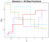
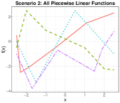
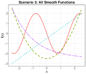
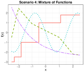
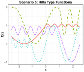
Figure 1: Plot of the 4 signal functions for each of the five simulation settings.

5 Simulation Study

In this section we conduct a simulation study to compare estimators obtained by the following choices of smoothness penalty, $P_{st}(\cdot)$.

1. SpAM (Ravikumar et al., 2009). $P_{st}(f)=\mathbb{I}(f;\operatorname{span}\{\psi_{1},\ldots,\psi_{M}\})$ for $M\in\{3,6,10,20,30,50,80\}$. We use the SAM R-package (Zhao et al., 2014).

2. SSP (Meier et al., 2009). $P_{st}(f)=\sqrt{\int_{x}(f^{(2)}(x))^{2}\,dx}$, the Sobolev smoothness penalty (SSP). Given the lack of efficient software for this method, we implemented it using the algorithm and results of Section 3.

3. TF (Sadhanala and Tibshirani, 2018). $P_{st}(f)=\int_{x}|f^{(k+1)}(x)|\,dx$ for $k\in\{0,1,2\}$, trend filtering for additive models. We implemented this method using the algorithm of Section 3 where the univariate sub-problem (15) was solved using the R package glmgen (Arnold et al., 2014).

We simulate data for each of five simulation scenarios as follows: Given a sample size $n$ and a number of covariates $p$, we draw 50 different $n\times p$ training design matrices $X$ where each element is drawn from $\mathcal{U}(-2.5,2.5)$. We replicate each of the 50 design matrices 10 times leading to a total of 500 design matrices. The response is generated as $y_{i}=f_{1}(x_{i1})+f_{2}(x_{i2})+f_{3}(x_{i3})+f_{4}(x_{i4})+\varepsilon_{i}$ where $\varepsilon_{i}\sim\mathcal{N}(0,1)$. The remaining covariates are noise variables. We also generate an independent test set for each replicate with sample size $n/2$. We vary the sample size, $n\in\{100,200,\ldots,800\}$ and consider both, a low-dimensional ($p=6$) and high-dimensional ($p=100$) settings. We consider five different choices of the signal functions as shown in Figure 1.

We fit each method over a sequence of $50~{}\lambda$ values on the training set, and select the tuning parameter $\lambda^{*}$ which minimizes the test error ($\|y_{test}-\widehat{y}\|^{2}_{n}$). For the estimated model $\widehat{f}_{\lambda^{*}}$, we report the mean square error (MSE; $\|\widehat{f}_{\lambda^{*}}-f^{0}\|_{n}^{2}$) as a function of $n$.

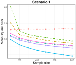
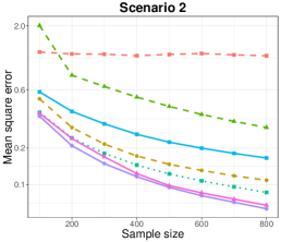
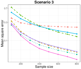
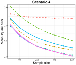
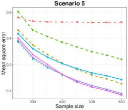
Figure 2: Plot of MSEs versus sample size for each of five scenarios for $p=6$, averaged over 500 replications. The dashed lines correspond to SpAM with small (), moderate () and high () number of basis functions. The solid lines correspond to trend filtering of order $k=0$ (), 1 () and 2 (). SSP is represented by the dotted line ().

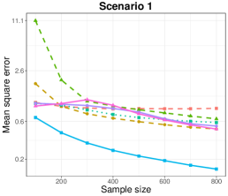
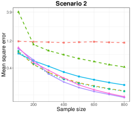
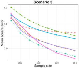
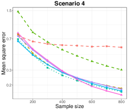
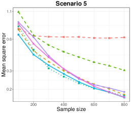
Figure 3: Plots of MSE versus sample size for each of five scenarios for $p=100$, averaged over 500 replications. The line types and colors are the same as in Figure 2.

In Figures 2 and 3, we plot the MSE as a function of $n$ for the low and high-dimensional setting, respectively. For each simulation scenario, we plot the performance of SpAM for three different choices of $M$ (low, moderate and high number of basis functions, $M$). In both low- and high-dimensional settings, we observe similar relative performances between the methods, with more variability in results for the high-dimensional setting. While there is no uniformly superior method, for all, except Scenario 1, the Sobolev smoothness penalty and trend filtering of orders 1 and 2 had comparably good performances. Unsurprisingly, trend filtering of order 0 exhibits superior performance in Scenario 1, where each component is piecewise constant. In each scenario, the bias-variance trade-off of SpAM depends on the choice of $M$: too small or large values of $M$ lead to high prediction error compared to other methods.

In Appendix LABEL:app:AdditionalFigures, we plot examples of fitted functions for the various methods. The dependence on $M$ for SpAM, is further illustrated in Figure LABEL:fig:SamplePlots, where we plot functions estimated by SpAM for high-dimensional Scenario 4 with $n=500$. We observe large bias for $M=3$ (especially for the piecewise constant and linear functions) and high variance for $M=30$. In the same figure, we also plot functions estimated by the SSP; SSP estimates exhibit a similar bias to that of SpAM with $M=10$, but with a substantially smaller variance. Figure LABEL:fig:SamplePlots2 similarly plots fitted example functions for trend filtering. Trend filtering with $k=0$ estimates the piecewise constant function well, but estimating the other $f_{j}$’s by piecewise constant functions incurs additional variance. Trend filtering with $k=1$ and $2$ estimates all other signal functions well.

6 Data Analysis

We use the methods of Section 5 to predict the value of owner-occupied homes in the suburbs of Boston using census data from 1970. The data consists of $n=506$ measurements and $10$ covariates, and has been studied in the additive models literature (Ravikumar et al., 2009; Lin and Zhang, 2006). As done in the data analysis by Ravikumar et al. (2009), we add 10 noise covariates uniformly generated on the unit interval and 10 additional noise covariates obtained by randomly permuting the original covariates.

We fit SSP, SpAM with $M=2$ and $3$ basis functions, and TF with orders $k=0,1,2$; we also fit the lasso Tibshirani (1996). Approximately $75\%$ of the observations are used as training set, and the mean square prediction error on the test set is reported. The final model is selected using 5-fold cross validation using the ‘1 standard error rule’. Results are presented for 100 splits of the data into training and test sets.

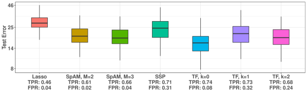
Figure 4: Box-plot of test errors for 100 different train/test splits of the data for each method. The average TPR and FPR was calculated using the original 10 covariates as ‘signal’ variables and remaining 20 as noise variables.

The box-plots of test error in the test set are shown in Figure 4. Since we added noise variables for the purpose of this analysis, we also state the average true positive rate (TPR) and false positive rate (FPR) in Figure 4. The box-plots demonstrate superior performance of TF of order $k=0$ over other methods in terms of lowest prediction error and highest TPR. The FPR of TF with $k=0$ is also low (under 10%). In Figure LABEL:fig:DataAnalysisExample of Appendix LABEL:app:AdditionalFigures, we plot fitted functions for one split of the data for lasso, SpAM with $M=3$, SSP and, TF with $k=0$ for the 10 covariates of the original dataset. A striking feature of TF fits is that many component functions are constant for extreme values of the covariates.

7 Conclusion

In this paper, we introduced a general framework for non-parametric high-dimensional sparse additive models. We show that many existing proposals, such as SpAM (Ravikumar et al., 2009), SPLAM (Lou et al., 2016), Sobolev smoothness (Meier et al., 2009), and trend filtering additive models (Sadhanala and Tibshirani, 2018; Petersen et al., 2016), fall within our framework.

We established a proximal gradient descent algorithm which has a lasso-like per-iteration complexity for certain choices of the structural penalty. Our theoretical analyses in Section 4 showed both fast rates, which match minimax rates under Gaussian noise, as well as slow rates, which only require a few weak assumptions.

The R package GSAM, available on https://github.com/asadharis/GSAM, implements the methods described in this paper.

See pages - of Supplement.pdf

References

- Arnold et al. [2014] Taylor Arnold, Veeranjaneyulu Sadhanala, and Ryan Tibshirani. glmgen: Fast algorithms for generalized lasso problems, 2014. R package version 0.0.3.
- Ayer et al. [1955] Miriam Ayer, H Daniel Brunk, George M Ewing, WT Reid, and Edward Silverman. An empirical distribution function for sampling with incomplete information. The Annals of Mathematical Statistics, 26(4):641–647, 1955.
- Beck and Teboulle [2009a] Amir Beck and Marc Teboulle. A fast iterative shrinkage-thresholding algorithm for linear inverse problems. SIAM Journal on Imaging Sciences, 2(1):183–202, 2009a.
- Beck and Teboulle [2009b] Amir Beck and Marc Teboulle. Gradient-based algorithms with applications to signal recovery. Convex Optimization in Signal Processing and Communications, pages 42–88, 2009b.
- Bühlmann and van de Geer [2011] Peter Bühlmann and Sara van de Geer. Statistics for high-dimensional data: methods, theory and applications. Springer Science & Business Media, 2011.
- Chouldechova and Hastie [2015] A. Chouldechova and T. Hastie. Generalized Additive Model Selection. ArXiv e-prints, June 2015.
- Dalalyan et al. [2017] Arnak S. Dalalyan, Mohamed Hebiri, and Johannes Lederer. On the prediction performance of the lasso. Bernoulli, 23(1):552–581, 2017.
- Fan et al. [2012] Jianqing Fan, Yang Feng, and Rui Song. Nonparametric independence screening in sparse ultra-high-dimensional additive models. Journal of the American Statistical Association, 2012.
- Friedman et al. [2010] Jerome H Friedman, Trevor J Hastie, and Robert J Tibshirani. Regularization paths for generalized linear models via coordinate descent. Journal of Statistical Software, 33(1):1–22, 2010.
- Hastie and Tibshirani [1990] Trevor J Hastie and Robert J Tibshirani. Generalized additive models, volume 43. CRC Press, 1990.
- Johnson [2013] Nicholas A Johnson. A dynamic programming algorithm for the fused lasso and l 0-segmentation. Journal of Computational and Graphical Statistics, 22(2):246–260, 2013.