Using two-dimensional Projections for Stronger Separation and Propagation of Bilinear Terms

Abstract

One of the most fundamental ingredients in mixed-integer nonlinear programming solvers is the well-known McCormick relaxation for a product of two variables $x$ and $y$ over a box-constrained domain. The starting point of this paper is the fact that the convex hull of the graph of $xy$ can be much tighter when computed over a strict, non-rectangular subset of the box. In order to exploit this in practice, we propose to compute valid linear inequalities for the projection of the feasible region onto the $x$-$y$-space by solving a sequence of linear programs akin to optimization-based bound tightening. These valid inequalities allow us to employ results from the literature to strengthen the classical McCormick relaxation. As a consequence, we obtain a stronger convexification procedure that exploits problem structure and can benefit from supplementary information obtained during the branch-and bound algorithm such as an objective cutoff. We complement this by a new bound tightening procedure that efficiently computes the best possible bounds for $x$, $y$, and $xy$ over the available projections. Our computational evaluation using the academic solver SCIP exhibit that the proposed methods are applicable to a large portion of the public test library MINLPLib and help to improve performance significantly.

1 Introduction

This paper is concerned with solving nonconvex mixed-integer quadratically constrained programs (MIQCPs) of the form

$$\min c^{\mathsf{T}}x$$ (1)

s.t. $$x^{\mathsf{T}}Q_{k}x+q_{k}^{\mathsf{T}}x\leq b_{k} \text{ for all }k\in\mathcal{M},$$

$$\ell_{i}\leq x_{i}\leq u_{i} \text{ for all }i\in\mathcal{N},$$

$$x_{i}\in\mathbb{Z} \text{ for all }i\in\mathcal{I},$$

where $\mathcal{N}:=\{1,\ldots,n\}$ is the index set of variables, $\mathcal{M}:=\{1,\ldots,m\}$ the index set of constraints,  $c\in\mathbb{R}^{n}$ is the objective function vector, $\ell\in\mathbb{R}^{n}$ and $u\in\mathbb{R}^{n}$ are the vectors of lower and upper bounds of the variables, $\mathcal{I}\subseteq\mathcal{N}$ is the index set of integer variables, and $Q_{k}\in\mathbb{R}^{n\times n}$ is a symmetric matrix for each $k\in\mathcal{M}$. Many real-world applications are inherently nonlinear and need to be tackled as MIQCPs or general mixed-integer nonlinear programs (MINLPs) that include quadratic constraint functions. For a selection see, e.g., [23]. In this article, we develop new convexification and bound tightening techniques that are directly relevant to achieve improvements within the algorithmic framework of spatial branch-and-bound, which forms the basis of many modern solvers in global optimization, e.g., ANTIGONE [7], BARON [48], Couenne [17], and SCIP [49].

For clarity of presentation we assume that the MIQCP is equivalently reformulated as

$$\min c^{\mathsf{T}}x$$ (2)

s.t. $$\langle X,Q_{k}\rangle+q_{k}^{\mathsf{T}}x\leq b_{k} \text{ for all }k\in\mathcal{M},$$

$$\ell_{i}\leq x_{i}\leq u_{i} \text{ for all }i\in\mathcal{N},$$

$$x_{i}\in\mathbb{Z} \text{ for all }i\in\mathcal{I},$$

$$X=xx^{\mathsf{T}}.$$

This reformulation is obtained by linearizing the original quadratic constraints via auxiliary variables and new constraints of the form $X_{ij}=x_{i}x_{j}$ for $i,j\in\mathcal{N}$. Usually, these constraints are only added for those $i,j\in\mathcal{N}$ for which $x_{i}x_{j}$ appears in at least one of the quadratic constraints of (1), i.e., if $(Q_{k})_{ij}\neq 0$ for some $k\in\mathcal{M}$. Formulation (2) is of major importance when using convex relaxations for solving MIQCPs to global optimality and allows us to focus on tight relaxations for the elementary nonconvex constraints of the form $X_{ij}=x_{i}x_{j}$ with $i\neq j$. The techniques presented in this paper extend fully to such bilinear constraints present in general reformulations that are applied when solving factorable MINLPs to global optimality [47, 53, 13]. For example, when a nonlinear constraint of the form $f(x)\,g(x)\leq d$ is reformulated as

$$w_{1}=f(x),\;w_{2}=g(x),\;w_{1}w_{2}\leq d,$$ (3)

with auxiliary variables $w_{1},w_{2}\in\mathbb{R}$, our results can be directly applied to improve the convexification and propagation of the product $w_{1}w_{2}$.

Our initial motivation is as follows. Classically, a linear relaxation for the nonconvex constraint $X_{ij}=x_{i}x_{j}$, $i\not=j$, is constructed by adding the four inequalities

$$X_{ij} \geq u_{j}x_{i}+u_{i}x_{j}-u_{i}u_{j},$$ (4)

$$X_{ij} \geq\ell_{j}x_{i}+\ell_{i}x_{j}-\ell_{i}\ell_{j},$$

$$X_{ij} \leq u_{j}x_{i}+\ell_{i}x_{j}-\ell_{i}u_{j},$$

$$X_{ij} \leq\ell_{j}x_{i}+u_{i}x_{j}-u_{i}\ell_{j},$$

often called McCormick inequalities [39]. These inequalities are best possible on the domain $[\ell_{i},u_{i}]\times[\ell_{j},u_{j}]$ in the sense that they describe the convex and concave envelope of $x_{i}x_{j}$ [3]. However, they do not take into account the presence of other linear and nonlinear inequalities of (2).

Suppose that for all feasible points $(x,X)$ of (2) the points $(x_{i},x_{j})$ are contained in a polytope $P$ that is a strict subset of $[\ell_{i},u_{i}]\times[\ell_{j},u_{j}]$. As can be seen in Figure 1a, the convex hull of the graph of $x_{i}x_{j}$ over $P$ is not given by (4) and is not polyhedral. Tangent inequalities for the convex and concave envelope of $x_{i}x_{j}$ over $P$ lead to a stronger linear relaxation of $X_{ij}=x_{i}x_{j}$ than (4).

(a) Improving separation: Two functions that are valid underestimators for $x_{i}x_{j}$ (orange) on a polyhedral domain (cyan). The figure shows that a linearization of the convex envelope (blue) at a given point (yellow) is locally tighter than the McCormick relaxation (gray).

(b) Improving propagation: The colored plot shows $x_{i}x_{j}$ over the polytope $P=[0,1]^{2}\cap\{(x_{i},x_{j})\mid x_{i}+x_{j}\leq\frac{3}{2}\}$ (cyan). The yellow point corresponds to the best possible bound of $x_{i}x_{j}$ on $P$, which is better than the best possible bound implied by the McCormick relaxation (4) on $P$ (green point).

Figure 1: Both separation and propagation can be improved by exploiting the presence of a non-rectangular, polyhedral domain.

In addition to tighter underestimators, knowledge about $P$ can be exploited to construct tighter variable bounds. For example, consider the polytope

$$P=\{(x_{i},x_{j})\in[0,1]^{2}\mid x_{i}+x_{j}\leq 3/2\}.$$ (5)

The best possible upper bound for $X_{ij}=x_{i}x_{j}$ over $P$ is given as

$$\max\{X_{ij}\mid(x_{i},x_{j})\in P,\,X_{ij}=x_{i}x_{j}\}=\frac{9}{16}.$$ (6)

This improves upon the upper bound implied by the McCormick relaxation over $P$,

$$\max\{X_{ij}\mid(x_{i},x_{j})\in P,\eqref{eq:mccormick}\}=\frac{3}{4}.$$ (7)

An illustration is given in Figure 1b.

These two examples show that a two-dimensional polytope $P\subsetneq[\ell_{i},u_{i}]\times[\ell_{j},u_{j}]$ for $(x_{i},x_{j})$ can be exploited in order to improve the convexification and propagation of $X_{ij}=x_{i}x_{j}$. In order to leverage this potential in practice, one needs to determine how to efficiently compute

1. a suitable polytope $P$,

2. tangent inequalities for the convex and concave envelope of $x_{i}x_{j}$ over $P$, and

3. tighter variable bounds for $x_{i}$, $x_{j}$, and $X_{ij}$ over $P$.

For the second step, an algorithm to compute tangent inequalities for the envelopes of $x_{i}x_{j}$ over $P$ is presented in the recent paper by Locatelli [36]. One requirement of this algorithm is that $P$ needs to be explicitly given, as output of step one.

Ideally, the original formulation (2) already contains inequalities that only depend on the two variables of a bilinear term. A good example are symmetry-breaking inequalities in circle packing problems. For example, the instance pointpack08 from the MINLPLib [42] test library contains constraints of the form

$$(x_{1}-x_{2})^{2}+(y_{1}-y_{2})^{2} \geq 1,$$ (8)

$$x_{1}-x_{2} \leq 0,$$

$$(x_{1},x_{2},y_{1},y_{2}) \in[0,1]^{4}.$$

Here $(x_{1},y_{1})$ and $(x_{2},y_{2})$ are the centers of two circles. The quadratic constraint ensures a minimum distance between these centers and the linear constraint orders them along the $x$-axis. In this case the inequality $x_{1}\leq x_{2}$ can be directly used for convexifying $x_{1}x_{2}$ with Locatelli’s algorithm.

However, for many instances inequalities only depending on variables of a single bilinear term may not appear in the initial formulation of the MIQCP. Nevertheless, it might be possible that a substructure of (2) implies such inequalities. For example, consider the instance crudeoil_lee1_05 from MINLPLib. Aggregating the linear constraints

$$x_{260}+x_{292}+x_{324}+x_{356}+x_{451} \leq 50,$$ (9)

$$-x_{394}+x_{525}+x_{526}+x_{527} =0,$$

$$x_{260}+x_{292}+x_{324}+x_{451}+x_{527} =50,$$

$$x_{525} \geq 0,$$

$$x_{526} \geq 0,$$

with the multiplier vector $(-\frac{1}{3},-\frac{1}{3},\frac{1}{3},\frac{1}{3},\frac{1}{3})$ shows that $x_{356}\leq x_{394}$ is valid and thus it can be used for strengthening the relaxation of $X_{356,394}=x_{356}\,x_{394}$.

In this spirit, the first contribution of this paper is a fully general scheme for computing projected relaxations $P$ in step one above. It solves a sequence of linear programs (LPs) to compute a polyhedral relaxation of the projection of the feasible region onto the space of two variables that appear bilinearly. The computed two-dimensional relaxation is described by at most eight inequalities. Second, we introduce a bound tightening procedure for forward and backward propagation that solves a reduced nonconvex optimization problem. This results in the best possible bounds for a bilinear term and its variables using the linear inequalities of the two-dimensional projection. Due to the construction of the projections, these optimization problems can be solved by inspecting only a constant number of points. Last, we propose an effective way of incorporating these techniques into an LP-based spatial branch-and-bound solver and provide a detailed computational analysis of their impact.

The remainder of the paper is organized as follows. Section 2 discusses relevant literature and provides an overview of convex relaxations for (2). In Section 3, we present a procedure for computing valid inequalities for the projections of the feasible region onto the space of two variables. Section 4 is dedicated to a bound tightening algorithm that exploits the computed projections. Section 5 provides a thorough computational study using the MINLP solver SCIP on publicly available benchmark instances based on three experiments. First, we measure the basic potential of the methods by analyzing how many instances of MINLPLib actually admit non-trivial two-dimensional projections. Second, we study the dual bound improvement in the root node of the branch-and-bound tree. Third, we evaluate the overall performance impact of the new methods on the full spatial branch-and-bound search. Section 6 gives concluding remarks.

2 Background

In this section, we give a brief overview of the relevant literature. First, we review important convex relaxations for MIQCPs and existing convexification methods for special nonconvex functions over non-rectangular domains. Second, we discuss basic bound tightening algorithms and their relation to convexification methods. Finally, we give a short summary of Locatelli’s algorithm and its complexity.

Convex relaxations for MIQCPs

Two important convex relaxations for MIQCPs that have been exhaustively studied in the literature are semidefinite programming (SDP) [55] and the reformulation-linearization technique (RLT) [51]. Both relaxations utilize the $X_{ij}$ variables of (2) in order to linearize $x_{i}x_{j}$. For an SDP relaxation the nonconvex constraint $X=xx^{\mathsf{T}}$ is relaxed to the convex constraint $X\succeq xx^{\mathsf{T}}$, which is equivalent to

$$\begin{bmatrix}1&x^{\mathsf{T}}\\ x&X\end{bmatrix}\succeq 0,$$

via the Schur complement [15]. Even though the resulting SDP relaxation is efficiently solvable in theory, optimizing SDPs in practice is a numerically challenging task. We refer to [44, 20, 24, 33, 38, 11] for applications which utilize SDP relaxations to solve quadratic optimization problems.

While the construction of an SDP relaxation is independent of any linear or linearized constraints, an RLT-based relaxation uses them directly. After introducing auxiliary variables $X\in\mathbb{R}^{n\times n}$ and the nonconvex constraints $X=xx^{\mathsf{T}}$, the idea is to linearize the product of all selections of two linear inequalities with the help of $X$. For example, consider the inequalities $x_{i}\geq 0$ and $\alpha^{\mathsf{T}}x-\alpha_{0}\geq 0$. Multiplying the second inequality by $x_{i}$ gives

$$\sum_{j=1}^{n}\alpha_{j}x_{i}x_{j}-\alpha_{0}x_{i}\geq 0,$$

which is linearized with $X$ to

$$\sum_{j=1}^{n}\alpha_{j}X_{ij}-\alpha_{0}x_{i}\geq 0.$$

These RLT inequalities can significantly improve a relaxation of (2), see [52, 40, 5]. Note that the McCormick relaxation (4) is a special form of RLT that uses variable bound constraints only.

To obtain a convex relaxation for (1), it is not mandatory to reformulate the MIQCP into (2). Following the ideas of McCormick [39], Vigerske [56] uses linear underestimators $\tilde{f}_{k}:[\ell,u]\rightarrow\mathbb{R}$ for each nonlinear function $f_{k}:[\ell,u]\rightarrow\mathbb{R}$ of a constraint $\sum_{k}f_{k}(x)\leq 0$ and obtains the valid cut $\sum_{k}\tilde{f}_{k}(x)\leq 0$ by summing the underestimators. The advantage of this approach is that it does not require the additional variables $X$ but Anstreicher [6] shows that even when replacing each quadratic function with its convex envelope, this is in general weaker than exploiting the extended formulation.

Convexification of bilinear terms

Although RLT-based relaxations utilize the LP relaxation, they do not necessarily describe the convex hull of the constraint $X_{ij}=x_{i}x_{j}$ over this relaxation. For example, consider the set

$$\{(x_{i},x_{j},X_{ij})\in[0,1]^{3}\mid X_{ij}=x_{i}x_{j},\,x_{i}\leq x_{j}\}.$$ (10)

The RLT relaxation of (10) is equal to

$$\{(x_{i},x_{j},X_{ij})\in[0,1]^{3}\mid\eqref{eq:mccormick},\,x_{i}^{2}\leq X_{ij}\},$$

when keeping the convex constraint $x_{i}^{2}\leq X_{ij}$. However, the convex hull of (10) is given by

$$\{(x_{i},x_{j},X_{ij})\in[0,1]^{3}\mid\eqref{eq:mccormick},\,x_{i}^{2}\leq(1+x_{i}-x_{j})X_{ij}\},$$

which is strictly tighter. This shows that RLT does not fully exploit the presence of linear inequalities.

In the literature, different cases for convexifying a bilinear term over special sets have been studied: Linderoth [35] proposed a branch-and-bound algorithm for solving nonconvex quadratically-constrained quadratic programs. Variables of a bilinear term are partitioned into two-dimensional triangles and rectangles. He characterized the convex and concave envelope of $x_{i}x_{j}$ over a triangular domain and used it to improve upon (4). Based on perspective functions, Hijazi [26] derived a closed formula for the convex and concave envelope on a polytope of the form $P:=\{(x_{i},x_{j})\in[\ell_{i},u_{i}]\times[\ell_{j},u_{j}]\mid x_{i}\leq x_{j}\}$. As mentioned above, an algorithm for computing tangent inequalities for the convex and concave envelope of $x_{i}x_{j}$ on a general two-dimensional polytope $P$ has been presented by Locatelli [36]. Instead of using information on $x_{i}$ and $x_{j}$, Miller et al. [41] showed a lifting procedure for cutting planes for $X_{ij}=x_{i}x_{j}$ that exploits bounds on $X_{ij}$ that are not implied by $x_{i}x_{j}$.

Bound tightening methods

As it is shown in (4), there is an interdependency between the variable bounds and the strength of the (convex) relaxation. Tighter variable bounds result in tighter relaxations for nonconvex constraints and vice versa. The two most practically relevant methods to tighten variable bounds are feasibility-based bound tightening (FBBT) and optimization-based bound tightening [46] (OBBT). FBBT is based on interval arithmetic, see, e.g., [12], and computes activities of nonlinear expressions over the domain of the variables (forward propagation) and conversely propagating the bounds on the constraint activities back to the bounds of the variables (reverse propagation). Implementations usually rely on the representation of nonlinear term as nodes of a directed acyclic expression graph, see [13] or [56] for details. OBBT computes tighter lower and upper bounds for a variable $x_{i}$ by minimizing and maximizing $x_{i}$ over a linear relaxation of (2). These two linear programs are called OBBT LPs. Computing the best possible bounds for all variables over a fixed linear relaxation requires solving $2n$ many OBBT LPs and thus OBBT is often too expensive to be applied in every node of a branch-and-bound tree. Gleixner et al. [21] show how dual solutions of OBBT LPs can be used during the tree search as a fast approximation of OBBT.

Locatelli’s algorithm

Let $P\subset\mathbb{R}^{2}$ be a polytope and let $(x_{i}^{*},x_{j}^{*})\in P$. Locatelli showed that computing a tangent inequality of the convex and concave envelope of $x_{i}x_{j}$ at $(x_{i}^{*},x_{j}^{*})$ reduces to selecting at most three points in the boundary of $P$ such that $(x_{i}^{*},x_{j}^{*})$ is contained in the convex hull of these points. Figure 2 shows all possible cases that can occur. The resulting inequality is determined by either

1. three vertices of $P$,

2. a vertex and a point $p$ on a facet of $P$ such that the inequality is tangent at $p$, or

3. two points $p$ and $q$ on different facets of $P$ such that the inequality is tangent at $p$ and $q$.

Locatelli derived closed formulas for computing the inequalities in each of the three cases. When $P=[\ell_{i},u_{i}]\times[\ell_{j},u_{j}]$, they collapse to the first case and yield the McCormick inequalities (4). The third case only occurs if $P$ is described by at least two non-axis parallel facets that have both a positive or both a negative slope.

To find a valid inequality that is also tangent to the convex (concave) envelope, one needs to iterate through all possible selections of the points as discussed above, and select the inequality that has the smallest (largest) value at $(x_{i}^{*},x_{j}^{*})$. The computational cost for iterating through all possible choices and computing the tangent inequality is

$$O\left(\begin{pmatrix}|V|\\ 3\end{pmatrix}+|V|\cdot|F|+\begin{pmatrix}|F|\\ 2\end{pmatrix}\right),$$

where $|V|$ is the number of vertices and $|F|$ be the number of facets of $P$ that are not axis-parallel.

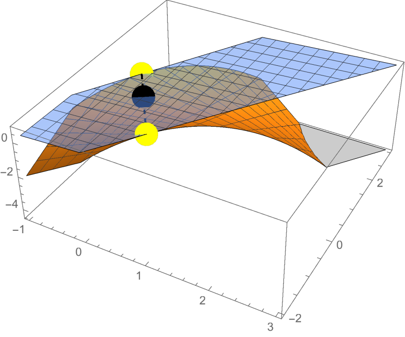
Figure 2: All possibilities for computing a tangent linear inequality (blue) for the convex and concave envelope of $x_{i}x_{j}$ on a two-dimensional polytope $P\subset\mathbb{R}^{2}$ at a given point (black). The inequality is obtained by selecting at most three points (yellow) that are on the boundary of $P$ such that the given point is in the convex hull of the selected points (dashed lines).

3 Two-dimensional projected relaxations

Consider a single nonconvex quadratic constraint $X_{ij}=x_{i}x_{j}$ of (2) with $i\neq j$, $x_{i}\in[\ell_{i},u_{i}]$, $x_{j}\in[\ell_{j},u_{j}]$, and $X_{ij}\in\mathbb{R}$. Let $\mathcal{F}$ be the set of feasible points of the original MINLP (2) and let

$$\mathcal{F}_{ij}:=\left\{(x_{i},x_{j})\mid x\in\mathcal{F}\right\}\subseteq[\ell_{i},u_{i}]\times[\ell_{j},u_{j}]$$ (11)

be the projection of $\mathcal{F}$ onto the $(x_{i},x_{j})$-space. The best possible convex relaxation for the nonconvex constraint $X_{ij}=x_{i}x_{j}$ is given by the convex hull of $\{(x_{i},x_{j},X_{ij})\in\mathcal{F}_{ij}\times\mathbb{R}\mid x_{i}x_{j}=X_{ij}\}$. However, it is unclear how to enforce this relaxation in practice. First, the set $\mathcal{F}$ is unknown and in general even finding a single point in $\mathcal{F}$ is $\mathcal{NP}$-hard. Second, $\mathcal{F}_{ij}$ can be a non-polyhedral, nonconvex, disconnected set and thus cannot be used by Locatelli’s algorithm. Hence, instead of targeting $\mathcal{F}_{ij}$ directly, we propose to compute a polyhedral relaxation $P_{ij}\subset\mathbb{R}^{2}$ of $\mathcal{F}_{ij}$, i.e., $\mathcal{F}_{ij}\subseteq P_{ij}$. This relaxation is based on a polyhedral relaxation of $\mathcal{F}$, which we denote by

$$\mathcal{X}:=\{(x,X)\mid A_{1}x+A_{2}X\leq d\},$$ (12)

where $X$ is assumed to be a vector. These relaxations are readily available in LP-based spatial branch-and-bound algorithms. They are constructed from linear constraints present in the original problem formulation, from cutting planes based on integrality information, and from other valid linearizations of quadratic constraints such as gradient cuts.

Similar to (11), let

$$\mathcal{X}_{ij}:=\left\{(x_{i},x_{j})\mid x\in\mathcal{X}\right\}\subseteq[\ell_{i},u_{i}]\times[\ell_{j},u_{j}]$$ (13)

be the projection of $\mathcal{X}$ onto the $(x_{i},x_{j})$-space. The best polyhedral relaxation from $\mathcal{X}$ is $\mathcal{X}_{ij}$. Unfortunately, exponentially many inequalities may be necessary to describe $\mathcal{X}_{ij}$ [14]. For this reason, exact projection methods such as standard homotopy procedures [43] may be overly expensive in practice. This motivates the computation of a relaxation $P_{ij}$ of $\mathcal{X}_{ij}$. In view of the complexity of Locatelli’s algorithm, we would like for $P_{ij}$ to have few vertices and facets. Specifically, we propose an algorithm that yields a $P_{ij}$ described by at most four axis-parallel and at most four general inequalities. Later, we show that the quotient of the volume of $\mathcal{X}_{ij}$ and the volume of the constructed $P_{ij}$ is bounded by $1/2$ from below.

Remark 1.

An even tighter relaxation can be achieved by also discarding feasible points from the set $\mathcal{F}$ by using an objective cutoff $c^{\mathsf{T}}x\leq\mathcal{U}$. Typically, solutions with an objective value $\mathcal{U}$ are found by heuristics during spatial branch-and-bound. Such a solution reduces the set of relevant feasible points to

$$\mathcal{F}\cap\{(x,X)\mid c^{\mathsf{T}}x\leq\mathcal{U}\},$$

which might later result in even tighter $P_{ij}$.

3.1 Computing polyhedral projections with linear programming

For $\mathcal{X}_{ij}\subsetneq[\ell_{i},u_{i}]\times[\ell_{j},u_{j}]$ to hold, there must be at least one valid (facet-defining) inequality that separates a vertex of $[\ell_{i},u_{i}]\times[\ell_{j},u_{j}]$ from $\mathcal{X}_{ij}$. To find some of those facets, if they exist, we follow a procedure akin to the shooting experiment [27]. The idea is to shoot a ray from a point $(C_{i},C_{j})\in\mathcal{X}_{ij}$ towards a vertex $(\bar{x}_{i},\bar{x}_{j})$ of $[\ell_{i},u_{i}]\times[\ell_{j},u_{j}]$. This ray is going to intersect the boundary of $\mathcal{X}_{ij}$. If the intersection is at the vertex, then the vertex is feasible for $\mathcal{X}_{ij}$. Otherwise, any active constraint at the intersection point separates the vertex from $\mathcal{X}_{ij}$. If the intersection point is in the interior of a facet, then that facet is the only active constraint. See Figure 3 for an illustration of the idea.

Figure 3: An example for computing heuristically one facet of $\mathcal{X}_{ij}$. The idea is to find a facet with minimum distance with respect to the line connecting the center with a vertex of $[\ell_{i},u_{i}]\times[\ell_{j},u_{j}]$. The red colored facet in the left picture is closest to the center among the three facets that separate the top-right vertex. The right picture shows that using this facet-defining inequality together with the bound constraints of $x_{i}$ and $x_{j}$ defines a polytope $P_{ij}$ which is a relaxation of $\mathcal{X}_{ij}$.

In our setting, the intersection point is $(x_{i}^{*},x_{j}^{*})$ where $(x^{*},X^{*},\theta^{*})$ is the solution of the following LP:

$$\max \theta,$$ (14)

s.t. $$A_{1}x+A_{2}X\leq d,$$

$$C_{i}+\theta(\bar{x}_{i}-C_{i})=x_{i},$$

$$C_{j}+\theta(\bar{x}_{j}-C_{j})=x_{j},$$

$$\theta\in\mathbb{R}.$$

Projecting out $\theta$ yields

$$\max \operatorname{sign}(\bar{x}_{i}-C_{i})x_{i},$$ (15)

s.t. $$A_{1}x+A_{2}X\leq d,$$

$$(x_{j}-C_{j})(\bar{x}_{i}-C_{i})=(x_{i}-C_{i})(\bar{x}_{j}-C_{j}),$$

which is in the following denoted by $\mbox{LP}(\bar{x}_{i},\bar{x}_{j})$. As is shown next, the dual solution of this LP can be utilized to construct the inequality we are looking for.

Let $(x^{*},X^{*},\lambda^{*},\mu^{*})$ be an optimal primal-dual solution of $\mbox{LP}(\bar{x}_{i},\bar{x}_{j})$, where $\lambda^{*}\geq 0$ are the dual multipliers of the inequality constraints and $\mu^{*}\in\mathbb{R}$ the dual multiplier for the equality constraint of (15). Note that the aggregation

$${\lambda^{*}}^{\mathsf{T}}(A_{1}x+A_{2}X)\leq{\lambda^{*}}^{\mathsf{T}}d$$

is valid for $\mathcal{X}$. Multiplying the stationarity condition

$$\operatorname{sign}(\bar{x}_{i}-C_{i})e_{i}^{\mathsf{T}}={\lambda^{*}}^{\mathsf{T}}\begin{pmatrix}A_{1}\\ A_{2}\end{pmatrix}+\mu^{*}\left(\frac{e_{i}^{\mathsf{T}}}{\bar{x}_{i}-C_{i}}-\frac{e_{j}^{\mathsf{T}}}{\bar{x}_{j}-C_{j}}\right)$$

of the Karush–Kuhn–Tucker [29, 31] conditions by $(x^{\mathsf{T}},X^{\mathsf{T}})^{\mathsf{T}}$ shows that

$$\operatorname{sign}(\bar{x}_{i}-C_{i})x_{i}={\lambda^{*}}^{\mathsf{T}}(A_{1}x+A_{2}X)+\mu^{*}\left(\frac{x_{i}}{\bar{x}_{i}-C_{i}}-\frac{x_{j}}{\bar{x}_{j}-C_{j}}\right)$$

holds. Using $A_{1}x+A_{2}X\leq d$ and reordering terms results in

$$\left(\operatorname{sign}(\bar{x}_{i}-C_{i})-\frac{\mu^{*}}{\bar{x}_{i}-C_{i}}\right)x_{i}+\frac{\mu^{*}}{\bar{x}_{i}-C_{i}}x_{j}\leq{\lambda^{*}}^{\mathsf{T}}d,$$ (16)

which is valid for $\mathcal{X}$ and only depends on $x_{i}$ and $x_{j}$ and is tight at the intersection point.

For having a complete method we need to specify $(C_{i},C_{j})\in\mathcal{X}_{ij}$. The center of $[\ell_{i},u_{i}]\times[\ell_{j},u_{j}]$ is guaranteed to be in $\mathcal{X}_{ij}$ after we applied OBBT on $x_{i}$ and $x_{j}$ for the relaxation $\mathcal{X}$, as the next Lemma shows. Recall that OBBT ensures $\ell_{i}=\min_{(x,X)\in\mathcal{X}}x_{i}$ and $u_{i}=\max_{(x,X)\in\mathcal{X}}x_{i}$.

Lemma 1.

Let $\mathcal{X}\neq\emptyset$, $\ell_{i}=\min_{(x,X)\in\mathcal{X}}x_{i}$, $u_{i}=\max_{(x,X)\in\mathcal{X}}x_{i}$, $\ell_{j}=\min_{(x,X)\in\mathcal{X}}x_{j}$, and $u_{j}=\max_{(x,X)\in\mathcal{X}}x_{j}$. Denote by

$$C:=\left(\frac{\ell_{i}+u_{i}}{2},\frac{\ell_{j}+u_{j}}{2}\right)$$

the center of $[\ell_{i},u_{i}]\times[\ell_{j},u_{j}]$. It holds that $C\in\mathcal{X}_{ij}$.

Proof.

Assume that $C\not\in\mathcal{X}_{ij}$. It follows that there is an inequality $\alpha_{i}x_{i}+\alpha_{j}x_{j}\leq\alpha_{0}$ that is valid for $\mathcal{X}_{ij}$ and separates $C$. The center $C$ can only be separated if the inequality separates at least two adjacent vertices of the rectangular domain $[\ell_{i},u_{i}]\times[\ell_{j},u_{j}]$. Assume that it separates $(\ell_{i},\ell_{j})$ and $(u_{i},\ell_{j})$ (all other three cases work analogously), i.e., $\alpha_{i}\ell_{i}+\alpha_{j}\ell_{j}>\alpha_{0}$ and $\alpha_{i}u_{i}+\alpha_{j}\ell_{j}>\alpha_{0}$. This immediately shows that there is no feasible point in $\mathcal{X}_{ij}$ with $x_{j}=\ell_{j}$, which is a contradiction to $\ell_{j}=\min_{(x,X)\in\mathcal{X}}x_{j}$ and $\mathcal{X}\neq\emptyset$. Figure 4 illustrates the idea of the proof. ∎

Figure 4: Idea of the proof of Lemma 1. The gray shaded area is the feasible region described by the inequality $\alpha_{i}x_{i}+\alpha_{j}x_{j}\leq\alpha_{0}$. The dashed line corresponds to a tighter lower bound on $x_{j}$ that is implied by the inequality.

Lemma 1 implies that each inequality that is valid for $\mathcal{X}_{ij}$ can separate at most one vertex of $[\ell_{i},u_{i}]\times[\ell_{j},u_{j}]$ directly after OBBT has been applied to $x_{i}$ and $x_{j}$. However, if tighter bounds from OBBT are used to strengthen the linear relaxation $\mathcal{X}$ further by, e.g., computing tighter convexifications for nonconvex constraints or propagating variables bounds via FBBT, then the conditions in Lemma 1 may not be met anymore. For this reason, we solve (15) immediately after OBBT.

Finally, we are able to define the polytope $P_{ij}$ by using the variable bounds $[\ell_{i},u_{i}]\times[\ell_{j},u_{j}]$ and the derived inequalities (16) for four choices of $\bar{x}_{i}$ and $\bar{x}_{j}$, namely the four vertices of $[\ell_{i},u_{i}]\times[\ell_{j},u_{j}]$. Defining $P_{ij}$ like this has the advantage that it is described by at most eight inequalities and covers at least half of the volume of $\mathcal{X}_{ij}$ as it is shown in the following section.

Remark 2.

The problem of computing a facet-defining inequality for a projection of a polyhedron has been extensively studied in the literature. It corresponds to the “project” step in lift-and-project cuts [9, 8]. The dual of (14) is

$$\max \beta-\alpha_{i}C_{i}-\alpha_{j}C_{j},$$ (17)

s.t. $$\alpha_{i}e^{\mathsf{T}}_{i}+\alpha_{j}e^{\mathsf{T}}_{j}=\lambda^{\mathsf{T}}A_{1},$$

$$0=\lambda^{\mathsf{T}}A_{2},$$

$$\beta=\lambda^{\mathsf{T}}d,$$

$$\alpha_{i}(\bar{x}_{i}-C_{i})+\alpha_{i}(\bar{x}_{i}-C_{i})=1,$$

$$\lambda\geq 0,$$

which can be interpreted as a cut generating linear program (CGLP) with the objective function of the so-called reverse polar CGLP [50, Chap. 2] and the normalization constraint of Balas and Perregaard [10]. We refer to the thesis of Serra [50, Chap. 2] for more details.

3.2 Volume bound

We are interested in how much we lose by not computing the exact projection of the polyhedral relaxation $\mathcal{X}$. In the literature, the volume has been used as a measure for the strength of relaxations, see [32, 54]. Following this line of thought, we provide a lower bound on the quotient of the volume of $\mathcal{X}_{ij}$ and $P_{ij}$.

Theorem 1.

Let $\mathcal{X}$ be a relaxation of 2 with $\ell_{i}=\min\{x_{i}\mid(x,X)\in\mathcal{X}\}$, $u_{i}=\max\{x_{i}\mid(x,X)\in\mathcal{X}\}$, $\ell_{j}=\min\{x_{j}\mid(x,X)\in\mathcal{X}\}$, $u_{j}=\max\{x_{j}\mid(x,X)\in\mathcal{X}\}$ for two variable indices $i,j\in\mathcal{N}$. Let $\mathcal{X}_{ij}=\{(x_{i},x_{j})\mid(x,X)\in\mathcal{X}\}$ be the two-dimensional projection of $\mathcal{X}$ onto the $(x_{i},x_{j})$-space. Let $P_{ij}$ be a polytope that is given by the intersection of $[\ell_{i},u_{i}]\times[\ell_{j},u_{j}]$ and (16) for the four choices $(\bar{x}_{i},\bar{x}_{j})\in\{\ell_{i},u_{i}\}\times\{\ell_{j},u_{j}\}$. Then, the inequality

$$\frac{\text{Vol}(\mathcal{X}_{ij})}{\text{Vol}(P_{ij})}\geq\frac{1}{2}$$

holds and the constant is best possible.

Proof.

Since the volume quotient is invariant with respect to scaling and translating, we assume that all variable bounds are $[0,1]$. By construction, $P_{ij}$ is a relaxation of $\mathcal{X}_{ij}$. Because the conditions of Lemma 1 are met, it follows that the center point $C=(1/2,1/2)$ belongs to $\mathcal{X}_{ij}$ and thus also to $P_{ij}$. Let $p^{k}\in\mathbb{R}^{2}$ for $k\in\{1,2,3,4\}$ be the four intersection points between $P_{ij}$ and the line connecting the center $C$. By construction, these four points belong to the set $\mathcal{X}_{ij}$.

First, we construct an example that shows that the constant is best possible. Let $(0,0)$, $(0,1-a)$, $(a,1)$, $(1,1)$, $(1,a)$, and $(1-a,0)$ be the vertices of $P_{ij}$ and $p^{1}=(0,0)$, $p^{2}=(a/2,1-a/2)$, $p^{3}=(1,1)$, $p^{4}=(1-a/2,a/2)$ the vertices of $\mathcal{X}_{ij}$ depending on a parameter $a\in[0,1]$. See Figure 5 for an illustration of the construction. It follows that $\text{Vol}(P_{ij})=1-a^{2}$ and $\text{Vol}(\mathcal{X}_{ij})=1-a$ holds. As a consequence,

$$\frac{\text{Vol}(\mathcal{X}_{ij})}{\text{Vol}(P_{ij})}=\frac{1-a}{1-a^{2}}=\frac{1-a}{(1-a)(1+a)}=\frac{1}{1+a}$$

converges to $\frac{1}{2}$ for $a\rightarrow 1$. Note that for $a=1$ the volume quotient exists but the polytopes $P_{ij}$ and $\mathcal{X}_{ij}$ reduce to a single line.

Now, we prove the inequality. Since $\mathcal{X}_{ij}$ is a subset of $P_{ij}$, it immediately follows that

$$\text{Vol}(P_{ij})=\text{Vol}(\mathcal{X}_{ij})+\text{Vol}(P_{ij}\backslash\mathcal{X}_{ij})\,.$$

The inequality $\text{Vol}(P_{ij}\backslash\mathcal{X}_{ij})\leq\text{Vol}(\mathcal{X}_{ij})$ is enough to show

$$\text{Vol}(P_{ij})=\text{Vol}(\mathcal{X}_{ij})+\text{Vol}(P_{ij}\backslash\mathcal{X}_{ij})\leq 2\cdot\text{Vol}(\mathcal{X}_{ij})\,,$$

which proves the theorem. We still need to prove the following claim.

Claim 1.

$\text{Vol}(P_{ij}\backslash\mathcal{X}_{ij})\leq\text{Vol}(\mathcal{X}_{ij})$

Proof.

Let $q^{k}\in\mathbb{R}^{2}$ for $k\in\{1,2,3,4\}$ be four points in $\mathcal{X}_{ij}$ such that each point touches a different side of the $[\ell_{i},u_{i}]\times[\ell_{j},u_{j}]$ box. The left picture in Figure 6 shows how the points are labeled. The set

$$X_{ij}^{\prime}:=\operatorname{conv}\{q^{1},p^{1},q^{2},p^{2},q^{3},p^{3},q^{4},p^{4}\}$$

is by construction a subset of $X_{ij}$. As $\text{Vol}(P_{ij}\backslash X_{ij}^{\prime})\leq\text{Vol}(P_{ij}\backslash X_{ij})$ and $\text{Vol}(X_{ij}^{\prime})\leq\text{Vol}(X_{ij})$, showing the claim for $X_{ij}^{\prime}$ implies the result for $X_{ij}$.

The set $X_{ij}^{\prime}$ decomposes into the four regions

$$R_{k}:=\operatorname{conv}\{C,q^{k},p^{k},q^{k+1}\}\subseteq X_{ij}^{\prime}$$

for $k\in\{1,2,3,4\}$, whereas $q^{5}=q^{1}$. The set $P_{ij}\backslash X_{ij}$ decomposes into eight triangles that are adjacent to the regions, see the right picture of Figure 6. In the following, we show that the area of each $R_{k}$ is at least as big as the area of the two corresponding triangles, which proves the claim.

Consider the region $R_{1}$ in the left-bottom corner. If $(a_{1},0)^{\mathsf{T}}$ and $(0,b_{1})^{\mathsf{T}}$ are the endpoints of the facet in $P_{ij}$ that contains $p^{1}=(c,c)^{\mathsf{T}}$, then $c=a_{1}\,b_{1}/(a_{1}+b_{1})$. Note that the claim is true if $a_{1}=0$ or $b_{1}=0$ because in this case the two adjacent triangles are empty. Let $q^{1}=(a_{2},0)^{\mathsf{T}}$ and $q^{2}=(0,b_{2})^{\mathsf{T}}$. The area of the triangle $\Delta_{1}:=\operatorname{conv}\{(a_{1},0)^{\mathsf{T}},p^{1},q^{1}\}\subseteq P_{ij}\backslash X_{ij}$ is

$$\text{Vol}(\Delta_{1})=\frac{c\,(a_{2}-a_{1})}{2}$$

and the area of the second triangle $\Delta_{2}:=\operatorname{conv}\{(0,b_{1})^{\mathsf{T}},p^{1},q^{2}\}\subseteq P_{ij}\backslash X_{ij}$ is

$$\text{Vol}(\Delta_{2})=\frac{c\,(b_{2}-b_{1})}{2}\,.$$

The area of the quadrilateral is given by the area of two triangles $\Delta_{3}=\operatorname{conv}\{C,p^{1},q^{1}\}$ and $\Delta_{4}=\operatorname{conv}\{C,q^{2},p^{1}\}$. Their areas are

$$\text{Vol}(\Delta_{3})=\frac{a_{2}}{4}-\frac{a_{2}\,c}{2}=\frac{a_{2}\,(1-2c)}{4}$$

and

$$\text{Vol}(\Delta_{4})=\frac{b_{2}}{4}-\frac{b_{2}\,c}{2}=\frac{b_{2}\,(1-2c)}{4}\,.$$

Finally, we show that the area of $\Delta_{1}$ and $\Delta_{2}$ is less or equal than the area of $\Delta_{3}$ and $\Delta_{4}$, which proves the claim. After algebraic manipulation, we get

$$\text{Vol}(\Delta_{1})+\text{Vol}(\Delta_{2}) -\text{Vol}(\Delta_{3})-\text{Vol}(\Delta_{4})=\frac{c\,(a_{2}-a_{1})}{2}+\frac{c\,(b_{2}-b_{1})}{2}-\frac{a_{2}\,(1-2c)}{4}-\frac{b_{2}\,(1-2c)}{4}$$

$$=\frac{-2a_{1}^{2}b_{1}-2a_{1}b_{1}^{2}+(a_{2}+b_{2})(4a_{1}b_{1}-a_{1}-b_{1})}{4(a_{1}+b_{1})}$$ (18)

where the second step used the definition of $c$, i.e., $c=a_{1}b_{1}/(a_{1}+b_{1})$. Since the denominator of (18) is positive, showing that the nominator of (18) is non-positive implies

$$\text{Vol}(\Delta_{1})+\text{Vol}(\Delta_{2}) -\text{Vol}(\Delta_{3})-\text{Vol}(\Delta_{4})\leq 0\,.$$

We consider two cases.

1. $4a_{1}b_{1}-a_{1}-b_{1}\leq 0$
   The nominator of (18) consists of three non-positive terms.

2. $4a_{1}b_{1}-a_{1}-b_{1}>0$
   Since $a_{2},b_{2}\in[0,1]$, it follows that

   $$-2a_{1}^{2}b_{1}-2a_{1}b_{1}^{2}+(a_{2}+b_{2})(4a_{1}b_{1}-a_{1}-b_{1}) \leq-2a_{1}^{2}b_{1}-2a_{1}b_{1}^{2}+2(4a_{1}b_{1}-a_{1}-b_{1})$$

   $$=2a_{1}(2b_{1}-b_{1}^{2}-1)+2b_{1}(2a_{1}-a_{1}^{2}-1)$$

   $$=-2a_{1}(b_{1}-1)^{2}-2b_{1}(a_{1}-1)^{2}\leq 0\,,$$

   which proves that the nominator of (18) is non-positive.

∎

∎

Figure 5: Construction of a parametric example that shows that $\frac{\text{Vol}(\mathcal{X}_{ij})}{\text{Vol}(P_{ij})}$ approaches $\frac{1}{2}$ when $a$ approaches $1$. The gray region is $\mathcal{X}_{ij}$ and the red region is $P_{ij}$.

Figure 6: Construction of $X_{ij}^{\prime}$ in the proof of Claim 1. The inner polytope is $X_{ij}^{\prime}$ (gray) is inscribed in $P_{ij}$. The main idea of the proof is that $P_{ij}\backslash X_{ij}$ (red) has smaller area than $X_{ij}$. The right picture illustrates that the region $R_{1}=\Delta_{3}\cup\Delta_{4}$ is larger than the two adjacent triangles $\Delta_{1}$ and $\Delta_{2}$.

Remark 3.

The construction of the parametric example in the proof of Theorem 1 requires that $P_{ij}$ contains two facets that are not axis-parallel. If only one facet of $P_{ij}$ is not axis-parallel, the volume quotient is bounded by $\frac{2+\sqrt{2}}{4}\approx 0.85$.

Theorem 1 and Remark 3 provide some theoretical justification why it suffices to compute a relaxation of the projection. From a practical point of view, spending more time in computing $\mathcal{X}_{ij}$ exactly might not pay off because we are only projecting a relaxation of the feasible region.

3.3 Computational aspects

So far, we have only considered a single term $x_{i}x_{j}$, but in general (2) contains up to $O(n^{2})$ many bilinear terms. With growing number of variables, it may become computationally too expensive to solve (15) for all bilinear terms. In order to save unnecessary solves of $\mbox{LP}(\bar{x}_{i},\bar{x}_{j},$), we observe the following: The existence of a feasible solution $(x^{*},X^{*})\in\mathcal{X}$ in which $(x_{i}^{*},x_{j}^{*})$ is a vertex of $[\ell_{i},u_{i}]\times[\ell_{j},u_{j}]$ proves that no useful inequality for $P_{ij}$ can be found that cuts off $(x_{i}^{*},x_{j}^{*})$. This observation is similar to the bound filtering in the branch-and-contract algorithm [59] and can be exploited as an aggressive filtering strategy, as it has been done in OBBT [21]. The idea of bound filtering is to use a solution $(x^{*},X^{*})$ of an LP relaxation $\mathcal{X}$ and to check for which variables $x_{i}$ the solution value $x_{i}^{*}$ is equal to $\ell_{i}$ or $u_{i}$. If $x_{i}^{*}=\ell_{i}$ ($x_{i}^{*}=u_{i}$) holds then OBBT cannot find a tighter lower (upper) bound for $x_{i}$. In addition to considering solutions from previous OBBT LPs, aggressive bound filtering solves auxiliary LPs with an objective function $v^{\mathsf{T}}x$ for a vector $v\in\{-1,0,1\}^{n}$ to push as many unfiltered variables as possible to their lower or upper bounds. We refer to [21] for more details.

In the following, we present the generic Algorithm 1 that first applies OBBT to ensure that the center point $(C_{i},C_{j})$ belongs to $\mathcal{X}_{ij}$ and afterwards computes a relaxation of $\mathcal{X}_{ij}$ as discussed above.

Algorithm 1 Two-dimensional projections

0:  linear relaxation $\mathcal{X}=\{(x,X)\mid A_{1}x+A_{2}X\leq d\}$ of (2)

0:  a list $\mathcal{P}$ of two-dimensional polytopes for each bilinear term $x_{i}x_{j}$

1:  $K\leftarrow\{(i,j)\in\mathcal{N}\times\mathcal{N}\mid i<j\land\exists k\in\mathcal{M}:(Q_{k})_{ij}\neq 0\}$  /* collect bilinear terms */

2:  $\mathcal{P}\leftarrow\emptyset$, $F\leftarrow\emptyset$

3:  for $i\in\mathcal{N}:\exists j\in\mathcal{N}$ such that $(i,j)\in K$ do  /* call OBBT */

4:     $[\ell_{i},u_{i}]\leftarrow$ apply OBBT on $x_{i}$; let $x^{*}$ be the OBBT LP solution

5:     $F\leftarrow F\,\cup\ \left\{(i^{\prime},j^{\prime},x_{i^{\prime}}^{*},x_{j^{\prime}}^{*})\mid(i^{\prime},j^{\prime})\in K\land x_{i^{\prime}}^{*}\in\{\ell_{i^{\prime}},u_{i^{\prime}}\}\land x_{j^{\prime}}^{*}\in\{\ell_{j^{\prime}},u_{j^{\prime}}\}\right\}$

6:  end for

7:  for $(i,j)\in K$ do

8:     $P_{ij}\leftarrow[\ell_{i},u_{i}]\times[\ell_{j},u_{j}]$

9:     for $(\bar{x}_{i},\bar{x}_{j})\in\{\ell_{i},u_{i}\}\times\{\ell_{j},u_{j}\}$ do  /* iterate through all vertices */

10:        if $(i,j,\bar{x}_{i},\bar{x}_{j})\not\in F$ then  /* consider unfiltered candidates */

11:           $(x^{*},X^{*},\lambda^{*},\mu^{*})\leftarrow$ solve $\mbox{LP}(\bar{x}_{i},\bar{x}_{j})$

12:           $F\leftarrow F\,\cup\ \left\{(i^{\prime},j^{\prime},x_{i^{\prime}}^{*},x_{j^{\prime}}^{*})\mid(i^{\prime},j^{\prime})\in K\land x_{i^{\prime}}^{*}\in\{\ell_{i^{\prime}},u_{i^{\prime}}\}\land x_{j^{\prime}}^{*}\in\{\ell_{j^{\prime}},u_{j^{\prime}}\}\right\}$

13:           if $x_{i}^{*}\neq\bar{x}_{i}\land x_{j}^{*}\neq\bar{x}_{j}$ then  /* create linear inequality */

14:              extract valid inequality (16) from dual solution $(\lambda^{*},\mu^{*})$

15:              $P_{ij}\leftarrow P_{ij}\,\cap\,\{(x_{i},x_{j})\mid\eqref{eq:projineq}\text{ holds}\}$

16:           end if

17:        end if

18:     end for

19:     add $P_{ij}$ to $\mathcal{P}$

20:  end for

21:  return  $\mathcal{P}$

In Line 1, Algorithm 1 computes an index set for all occurring bilinear terms. OBBT is called in Line 4 for each variable that appears bilinearly to ensure that the requirements of Lemma 1 are met. Afterward, in Line 11, for each term $x_{i}x_{j}$ the algorithm considers all vertices $(\bar{x}_{i},\bar{x}_{j})$ of $[\ell_{i},u_{i}]\times[\ell_{j},u_{j}]$ and solves $\mbox{LP}(\bar{x}_{i},\bar{x}_{j})$. The result is a primal-dual optimal solution $(x^{*},X^{*},\lambda^{*},\mu^{*})$ that is used in Line 14 for generating a valid inequality for $\mathcal{X}_{ij}$. The LP solutions from Line 4 and 11 are used to update the set of filtered candidates $F$ in Line 5 and 12. In Line 10, a candidate $(x_{i},x_{j})$ for the direction $(\bar{x}_{i},\bar{x}_{j})\in\{\ell_{i},u_{i}\}\times\{\ell_{j},u_{j}\}$ is only considered if $(i,j,\bar{x}_{i},\bar{x}_{j})$ has not been filtered out.

In our implementation, all bilinear terms are ordered by how often they appear in different constraints of the original MIQCP. As a tie-break, we use the term $x_{i}x_{j}$ for which the volume of $[\ell_{i},u_{i}]\times[\ell_{j},u_{j}]$, i.e., $(u_{i}-\ell_{i})(u_{j}-\ell_{j})$ is maximized.

Algorithm 1 could either solve $\mbox{LP}(\bar{x}_{i},\bar{x}_{j})$ or its dual formulation (17) for deriving the two-dimensional projections. However, solving $\mbox{LP}(\bar{x}_{i},\bar{x}_{j})$ has two technical advantages:

1. The linear relaxation $\mathcal{X}$ is available in LP-based spatial branch-and-bound solvers and only needs to be extended by a single linear equality constraint for solving $\mbox{LP}(\bar{x}_{i},\bar{x}_{j})$. This is beneficial compared to constructing (17) for a relaxation that contains many variables and constraints.

2. Due to the close connection to OBBT, it is possible to warm start from a previously computed basis of an OBBT-LP. This would require to restructure Algorithm 1 in a way that it solves $\mbox{LP}(\bar{x}_{i},\bar{x}_{j})$ after the bounds of $x_{i}$ and $x_{j}$ have been tightened by OBBT. However, restoring a previous LP basis causes a significant overhead that cannot be compensated by the warm start capabilities of the LP solver. For this reason, our implementation of Algorithm 1 does not utilize a previously computed LP basis.

After computing inequalities of the form (16), we apply Locatelli’s algorithm to strengthen the linear relaxation of $X_{ij}=x_{i}x_{j}$ through separation during the tree search. Moreover, the computed $P_{ij}$ can not only be used to improve separation but also to strengthen variable bounds of $X_{ij}$, $x_{i}$, and $x_{j}$, as shown in the next section.

4 Using 2D projections for propagation

Tight variable bounds are crucial when computing linear (or convex) relaxations for MIQCPs during spatial branch-and-bound. Stronger bounds on $x_{i}$, $x_{j}$, and $X_{ij}$ not only affect the relaxation of $X_{ij}=x_{i}x_{j}$ but also other constraints that involve these variables, including linear constraints. Propagating these constraints in turn might lead to further bound reductions of variables that appear in other nonconvex constraints [12, 45] and subsequently result in tighter relaxations.

In the following, we show how to use a two-dimensional projection $P_{ij}$ to derive tighter bounds on $x_{i}$, $x_{j}$, and $X_{ij}$ by solving nonconvex optimization problems that can be efficiently solved.

4.1 Forward propagation

Given a polytope $P_{ij}$, the best possible lower/upper bound for $X_{ij}$ on $P_{ij}$ is given by

$$\min/\max\{X_{ij}\mid X_{ij}=x_{i}x_{j},\,(x_{i},x_{j})\in P_{ij}\},$$ (19)

which is a nonconvex optimization problem. Denote by $F(P_{ij})$ the facets of $P_{ij}$, and let

$$C(P_{ij}):=\left\{\operatorname*{argmax}_{(x_{i},x_{j})\in F}x_{i}x_{j}\mid F\in F(P_{ij})\right\}\cup\left\{\operatorname*{argmin}_{(x_{i},x_{j})\in F}x_{i}x_{j}\mid F\in F(P_{ij})\right\}$$

be the set of optimal points for maximizing and minimizing $x_{i}x_{j}$ over each facet of $P_{ij}$. For example, if $F=\{(x_{i},x_{j})\in[\ell_{i},u_{i}]\times[\ell_{j},u_{j}]\mid a_{i}x_{i}+a_{j}x_{j}=a_{0}\}$ is a facet of $P_{ij}$ with $a_{i}\neq 0$ and $a_{j}\neq 0$, then $x_{i}x_{j}$ restricted to $F$ is $-\frac{a_{i}}{a_{j}}x_{i}^{2}+\frac{a_{0}}{a_{j}}x_{i}$. The critical point of this function is $\frac{a_{0}}{2a_{i}}$. Thus $(\frac{a_{0}}{2a_{i}},\frac{a_{0}}{2a_{j}})\in C(P_{ij})$ if and only if $\frac{a_{0}}{2a_{j}}\in[\ell_{i},u_{i}]$ and $\frac{a_{0}}{2a_{i}}\in[\ell_{j},u_{j}]$. Otherwise, both vertices of $F$ belong to $C(P_{ij})$.

See Figure 7 for an illustration of the points $C(P_{ij})$. The following theorem shows that (19) can be solved by computing the minimum / maximum on the discrete set $C(P_{ij})$.

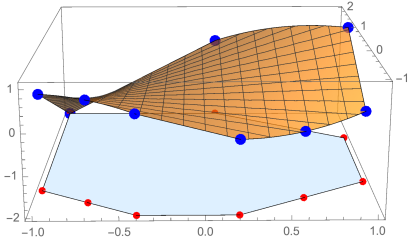
Figure 7: An example of how to compute the minimum and maximum of $x_{i}x_{j}$ on $P_{ij}\subset[-1,1]\times[-1,2]$. The red points are the points in $C(P_{ij})$.

Theorem 2.

Let $P_{ij}\subset\mathbb{R}^{2}$ be a polytope and let $C(P_{ij})$ be the optimal points of $P_{ij}$. Then the equality

$$\min\{\alpha x_{i}x_{j}\mid(x_{i},x_{j})\in P_{ij}\}=\min\{\alpha x_{i}x_{j}\mid(x_{i},x_{j})\in C(P_{ij})\}$$

holds for $\alpha\in\{-1,1\}$.

Proof.

First, due to the fact that $x_{i}x_{j}$ is bilinear, the minimum and maximum must be attained at the boundary of $P_{ij}$. Restricted to a facet, $x_{i}x_{j}$ achieves its maximum and minimum at a point in $C(P_{ij})$. ∎

By construction, $P_{ij}$ has at most four facets that are not axis-parallel. This bounds the number of points in $C(P_{ij})$ by 12. Computing these points requires only simple algebraic computations as illustrated in the example above.

4.2 Reverse propagation

There are two ways to obtain tighter variable bounds for $x_{i}$ and $x_{j}$ by utilizing $P_{ij}$. First, after branching on $x_{i}$ or $x_{j}$, it is possible that a facet of $P_{ij}$ cuts off two vertices of the rectangular domain for some locally valid bounds. This implies that at least one of the variable bounds of $x_{i}$ or $x_{j}$ can be tightened.

Second, the bounds of $X_{ij}$ define a level set for the bilinear term $x_{i}x_{j}$. Intersecting the level set with $P_{ij}$ might imply tighter lower and upper bounds on $x_{i}$ and $x_{j}$. Even though the intersection is in general a nonconvex region, we show that the best possible variable bounds that are implied by the intersection can be computed by considering a finite set of points.

In the following, we give more details on the two possible types of bound reductions for $x_{i}$ and $x_{j}$.

Branching reductions

Even though the facets of $P_{ij}$ are valid and redundant inequalities for the relaxation $\mathcal{X}$ that has been used for computing $P_{ij}$, they are still useful for deriving bound reductions on $x_{i}$ and $x_{j}$ during the tree search. Figure 8 shows that $P_{ij}$ implies tighter bounds on $x_{j}$ after branching on $x_{i}$. Note that optimizing $\pm x_{j}$ over $\mathcal{X}$ leads to bounds that are at least as tight as the bounds implied by $P_{ij}$. However, finding these bounds either requires solving an expensive OBBT-LP or propagating several linear constraints with FBBT. The strength of using $P_{ij}$ together with variable bound changes due to branching is that the facets of $P_{ij}$ contain information of multiple inequalities of $\mathcal{X}$ and are computationally cheap to propagate. Using the facets of $P_{ij}$ in this fashion is very similar to the so-called Lagrangian Variable Bounds of Gleixner et al [22], which are aggregations of linear constraints that are learned during OBBT and used as a computationally cheap approximation for OBBT during the tree search.

Figure 8: The example shows that the upper bound of $x_{j}$ can be improved after using $x_{i}^{*}$ as branching point for $x_{i}$. The vertical red line is the branching point of $x_{i}$. The horizontal green lines correspond to a tighter lower bound $\ell_{j}^{\prime}$ and a tighter upper bound $u_{j}^{\prime}$ in both subproblems, respectively.

Level set reductions

Let $[\ell_{ij},u_{ij}]$ be bounds on $X_{ij}$ such that

$$\ell_{ij}>\min\{x_{i}x_{j}\mid(x_{i},x_{j})\in P_{ij}\}$$

or

$$u_{ij}<\max\{x_{i}x_{j}\mid(x_{i},x_{j})\in P_{ij}\}$$

holds. This means that the bounds on $X_{ij}$ are not implied by $x_{i}x_{j}$ on $P_{ij}$. The best possible lower/upper bound on $x_{i}$ (and analogous for $x_{j}$) using $P_{ij}$ and the bounds $[\ell_{ij},u_{ij}]$ is given by

$$\min/\max\left\{x_{i}\mid\ell_{ij}\leq x_{i}x_{j}\leq u_{ij},\,(x_{i},x_{j})\in P_{ij}\right\},$$ (20)

which is a nonconvex optimization problem. Figure 9 illustrates that intersecting the level set of $x_{i}x_{j}$ and $P_{ij}$ can imply stronger bounds on $x_{i}$ and $x_{j}$. Similar to Theorem 2, we show that (20) can be efficiently solved by scanning a finite set of points. Let $IP\subseteq P_{ij}$ consist of the vertices of $P_{ij}$ that satisfy $x_{i}x_{j}\in[\ell_{ij},u_{ij}]$, and the intersection points of each facet of $P_{ij}$ with $\{(x_{i},x_{j})\mid x_{i}x_{j}=\ell_{ij}\}$ or $\{(x_{i},x_{j})\mid x_{i}x_{j}=u_{ij}\}$. In other words, $IP$ is the set of feasible points for which at least two constraints of (20) are active. Since the vertices and facets of $P_{ij}$ are explicitly given, computing points in $IP$ reduces to solving a univariate quadratic equation.

The following theorem shows that it suffices to consider the points in $IP$ to solve (20).

Theorem 3.

Let $x_{i}x_{j}$ a bilinear term, $[\ell_{ij},u_{ij}]$ bounds on $x_{i}x_{j}$, and $P_{ij}\subseteq\mathbb{R}^{2}$ a polytope. Then the equality

$$\min\left\{\alpha x_{i}\mid\ell_{ij}\leq x_{i}x_{j}\leq u_{ij},\,(x_{i},x_{j})\in P_{ij}\right\}=\min\left\{\alpha x_{i}\mid(x_{i},x_{j})\in IP\right\}$$

holds for $\alpha\in\{-1,1\}$.

Proof.

We only prove the theorem for the objective function $x_{i}$ since $-x_{i}$ is analogous. Let $x_{i}^{*}$ be the optimal value. As the objective function is linear, every optimum is at the boundary. Therefore, at least one constraint it active. We will show that there is at least one optimum for which at least two constraints are active, i.e., is in $IP$. Let $(x_{i}^{*},x_{j}^{*})$ be any optimal point.

If the only active constraint is linear, then it must be $x_{i}\geq x_{i}^{*}$. Since the feasible region is bounded, there is an $M>0$ such that $(x_{i}^{*},x_{j}^{*}+M)$ is infeasible. Therefore, for some $x_{j}\in[x_{j}^{*},x_{j}^{*}+M]$, $(x_{i}^{*},x_{j})$ is active for at least two constraints.

If the only active constraint is nonlinear, say, $x_{i}x_{j}=\phi$ with $\phi\in\{\ell_{ij},u_{ij}\}$, then the region $\{(x_{i},x_{j}):x_{i}x_{j}=\phi\}$, in a neighborhood of $(x_{i}^{*},x_{j}^{*})$, must be contained in $x_{i}\geq x_{i}^{*}$. This can only happen when $x_{i}^{*}=0$ and the same argument as above shows that there is an $x_{j}$ such that $(x_{i}^{*},x_{j})$ is active for another constraint. ∎

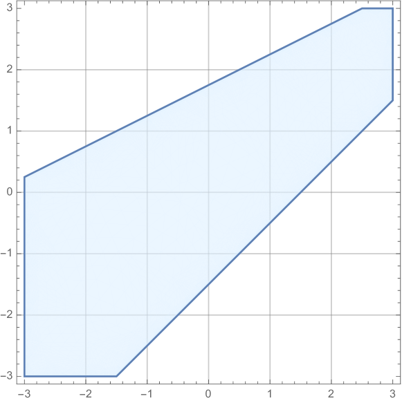
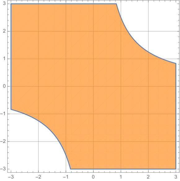
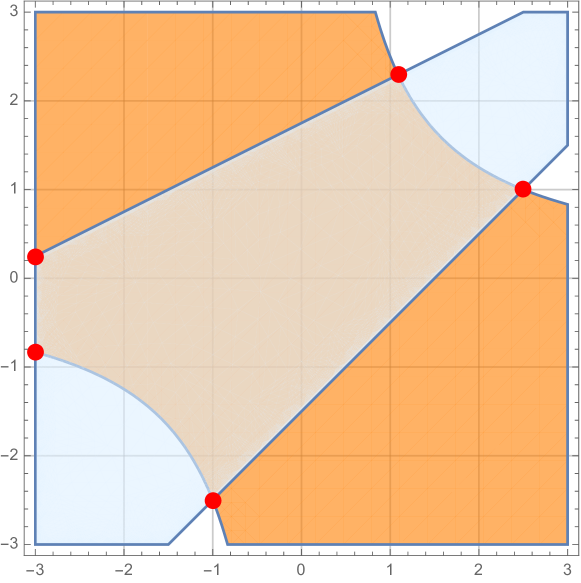
Figure 9: An example that shows bound reductions on $x_{i}$ and $x_{j}$ by utilizing $P_{ij}$ and bounds $[\ell_{ij},u_{ij}]$ on $X_{ij}$. The left plot shows $P_{ij}$, the middle plot shows the points $(x_{i},x_{j})$ that satisfy $x_{i}x_{j}\leq u_{ij}$, and the right plot the intersection of both sets. Optimizing in the unit directions of the intersection, i.e., minimizing and maximizing $x_{i}$ and $x_{j}$, is equivalent to optimizing over the red points.

5 Computational experiments

In this section, we present a computational study of the presented propagation and separation ideas for bilinear terms for publicly available instances of the MINLPLib [42]. We conduct three experiments to answer the following questions:

1. AFFECTED: Since it is unclear whether and to what extend MINLPs in practice allow for a nontrivial projection $\mathcal{X}_{ij}$, we first investigate empirically how many instances have a linear relaxation that provides inequalities of the form (16) that are not axis-parallel.

2. ROOTGAP: How much gap can be closed when using the stronger separation and propagation of bilinear terms only in the root node of a branch-and-bound tree with aggressive root separation settings?

3. TREE: How much do the presented techniques affect the solvability and performance of MINLPs in spatial branch-and-bound? For this experiment, we discuss suitable working limits on the number of LP iterations to solve the projections and investigate the performance impact of the stronger separation and propagation individually.

Our ideas are embedded in the MINLP solver SCIP [49]. We refer to [1, 56, 57] for an overview of the general solving algorithm and MINLP features of SCIP.

5.1 Experimental setup

For the AFFECTED and ROOTGAP experiments, we disable the LP iteration limit of the OBBT propagator, enable the aggressive separation emphasis setting, and disable restarts. The choices for the parameters ensure that the root node has been completely processed and there are no further reductions possible by applying OBBT again. Afterward, we use the current linear relaxation to compute the two-dimensional projections $P_{ij}$ as described in Algorithm 1. The projections are then used to strengthen the separation and propagation of constraints of the form $X_{ij}=x_{i}x_{j}$.

In contrast to the first two experiments, the TREE experiment is based on default settings. The projections are utilized at every node of the branch-and-bound tree. Note that the convex hull of the graph of $x_{i}x_{j}$ on $P_{ij}$ is in general not polyhedral. To prevent a potential slowdown caused by too many separation rounds, at local nodes of the branch-and-bound tree, i.e., not at the root node, we use the inequalities only twice for separation. Additionally, we use a limit on the total number of LP iterations in order to bound to computational cost of solving (15). Similarly to Gleixner et al. [21], a limit of three times the LP iterations that are spent so far at the root node is imposed.

For the AFFECTED and ROOTGAP experiments, we use a time limit of 7200s and a memory limit of 30 GB to ensure that for each instance the root node could be completely processed. For our TREE experiment, all instances run with a time limit of 1800s, a memory limit of 30 GB, and an optimality gap limit of $10^{-4}$ to reduce the impact of tailing-off effects.

Implementation

We extended two existing plug-ins of SCIP: the OBBT propagator, which can now additionally compute the two-dimensional projections for variables that appear in a bilinear term $x_{i}x_{j}$; and a so-called nonlinear handler that calls Locatelli’s algorithm and the propagation techniques described in Section 4 for each $x_{i}x_{j}$ individually. Bilinear terms that only appear in convex constraints or contain binary variables are ignored in both steps. To reduce side effects, we use a separate working limit for solving the LPs (15) after applying standard OBBT. This is similar to the structure of Algorithm 1.

Using OBBT in a local node of the tree search results in a significant slowdown of SCIP. For this reason, by default, SCIP applies OBBT only in the root node of the branch-and-bound tree.

Test set

We used the publicly available instances of the MINLPLib [42], which at time of the experiments contained 1682 instances. This includes among others instances from the first MINLPLib, the nonlinear programming library GLOBALLib, and the CMU-IBM initiative minlp.org [16]. We selected the instances that were available in OSiL format and consisted of nonlinear expressions that could be handled by SCIP: 1671 instances.

Hardware and software

The experiments were performed on a cluster of 64bit Intel Xeon X5672 CPUs at 3.2 GHz with 12 MB cache and 48 GB main memory. In order to safeguard against a potential mutual slowdown of parallel processes, we ran only one job per node at a time. We used a development version of SCIP that is based on version 6.0 with CPLEX 12.8.0.0 as LP solver [28], CppAD 20180000.0 [19], and Ipopt 3.12.11 as NLP solver [58, 18] with Mumps 4.10.0 [4].

Averages and statistical tests

In order to evaluate algorithmic performance over a large set of benchmark instances, we compare geometric means, which provide a measure for relative differences. This avoids results being dominated by outliers with large absolute values as is the case for the arithmetic mean. In order to also avoid an over-representation of differences among very small values, we use the shifted geometric mean. The shifted geometric mean of values $v_{1},\ldots,v_{N}\geq 0$ with shift $s\geq 0$ is defined as

$$\left(\prod_{i=1}^{N}(v_{i}+s)\right)^{1/N}-s.$$

See also the discussion in [1, 2, 25]. We use a shift value of $100$ for LP iterations and a value of one second for the solving time.

5.2 Computational results

In the following, we present results for the three above described experiments.

AFFECTED experiment.

In order to quantify how many instances are potentially affected by our ideas, we use the number of bilinear terms for which a useful two-dimensional projection could be found after processing the root node. We prioritize bilinear terms that appear in multiple quadratic constraints. In our analysis this is captured by taking the occurrence of a bilinear term in the original MIQCP (1) into account. Denote by

$$K_{ij}:=|\{k\in\mathcal{M}\mid(Q_{k})_{ij}\neq 0\}|$$

the number of constraints in (1) that contain $x_{i}x_{j}$. The value $\phi_{ij}\in\{0,1\}$ indicates whether a useful projection could be found for $x_{i}x_{j}$ or not. Then

$$\Psi:=\frac{\sum_{i,j}K_{ij}\phi_{ij}}{\sum_{i,j}K_{ij}}\in[0,1]$$

defines a measure for the effectiveness of an MIQCP. The interpretation of $K_{ij}$ in the definition of $\Psi$ is that each bilinear term $x_{i}x_{j}$ is counted as a separate term of (1).

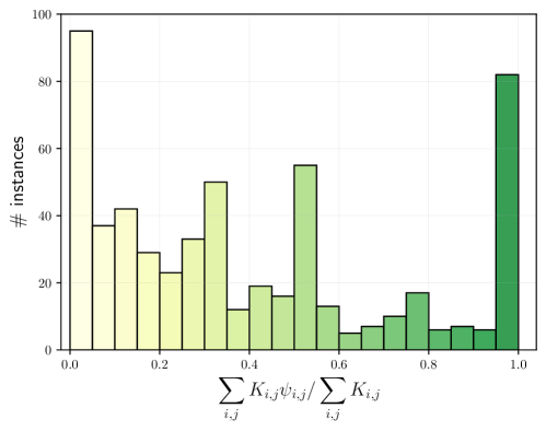
Figure 10: Instances of the MINLPLib that contain at least one bilinear term $x_{i}x_{j}$ for which the two-dimensional projection is not equal to $[\ell_{i},u_{i}]\times[\ell_{j},u_{j}]$. The y-axis displays the total number of instances and the x-axis an interval effectiveness $\Psi\in[0,1]$.

Figure 10 shows the effectiveness on the instances of the MINLPLib, where instances with $\Psi=0$ are filtered out. Detailed results for all instances that contain at least one bilinear term are given in Table LABEL:table:affected:detailed of the electronic supplement. Out of the 1682, 464 do not contain a bilinear term or are solved before computing the two-dimensional projections. In total, 564 instances provide a relevant projection for at least one bilinear term, i.e., $\Psi>0$. There are 97 instances with an effectiveness between $0-5$% and 82 instances with an effectiveness of $95-100$%. The average effectiveness among all instances is 0.19 and 0.40 for the subset of instances that have a strictly positive effectiveness.

Note that although we do not use an exact algorithm for computing the projection, we obtain the same number of relevant instances because if no nontrivial facet was found then the box is the exact projection, i.e, $[\ell_{i},u_{i}]\times[\ell_{j},u_{j}]=\mathcal{X}_{ij}$.

To analyze the computational cost of computing all projections, we use the total number of LP iterations and the time spent for solving all LPs (15). Computing all projections takes on average 2.6 seconds and 4454.6 LP iterations. On instances that do not provide any useful projection, we observe on average 875.3 LP iterations and spend 1.0 seconds in computing the projections. This time can be considered to be a constant slow-down because we could not learn anything for these instances which could pay off in the remaining solution process. For instances with a strict positive effectiveness, we use on average 9374.3 LP iterations and 3.6 seconds.

We briefly report on the success of filtering candidates by exploiting previously computed LP optima in Line 5 and 12 of Algorithm 1. Out of all 1682 instances, we could filter candidates on 797 instances. On these instances, the filtering rate is on average 48.1% and 51.0% on the 564 selected instances.

Last, we report on the impact of finding nontrivial inequalities when applying Algorithm 1 multiple times in the root node. As discussed in Section 3.1, tighter projections could be found when refining $\mathcal{X}$ after calling OBBT. Indeed, we observed a slight improvement in the success when recomputing the projections. The first bar of Figure 10 decreases from $97{}$ to $87$, which means that for $10$ more instances a relevant projection could be found that could not be found before. The average effectiveness improves from $18.9$% to $19.2$% on all instances, and improves from $40.3$% to $41.0$% on the affected instances.

Even though there is a slight improvement in the success when recomputing the projections in the root node, we observed that the tighter projections have almost no impact on the dual bounds of the ROOTGAP experiment. Due to the fact that recomputing the projections can be expensive, we only use Algorithm 1 once in the root node.

ROOTGAP experiment

Aggregated results for the ROOTGAP experiment are shown in Table 1 and visualized in Figure 11. We refer to Table LABEL:table:root:detailed in the electronic supplement for detailed, instance-wise results.

From the potentially 564 affected instances of the previous experiment, we filtered out all instances that have been detected to be infeasible, no primal solution is known, or we could not prove any finite dual bound with the above described settings. This leaves $547$ instances. Let $I:=\{1,\ldots,$547${}\}$ be the index set of these instances.

Definition 1.

Let $p\in\mathbb{R}$ be a valid primal bound and $d_{1}\in\mathbb{R}$ and $d_{2}\in\mathbb{R}$ be two dual bounds for (1), i.e., $d_{1}\leq p$ and $d_{2}\leq p$. The function $GC:\mathbb{R}^{3}\rightarrow[-1,1]$ with

$$GC(p,d_{1},d_{2}):=\begin{cases}0,&\text{ if }d_{1}=d_{2}\\ +1-\frac{p-d_{1}}{p-d_{2}},&\text{ if }d_{1}>d_{2}\\ -1+\frac{p-d_{2}}{p-d_{1}},&\text{ if }d_{1}<d_{2}\end{cases}$$

measures the gap closed improvement when comparing the distance of $d_{1}$ and $d_{2}$ to $p$.

Denote by $d_{1}^{i}$ and $d_{2}^{i}$ the dual bounds of instance $i\in I$ obtained with and without using the two-dimensional projections for separation and propagation. A reference primal bound $p^{i}$ is given by the best known bound for $i\in I$ in the MINLPLib. We use the gap-closed values for comparing the bounds $d_{1}^{i}$ and $d_{2}^{i}$ with respect to $p^{i}$. Note that $GC(d_{1}^{i},d_{2}^{i},p^{i})=1$ implies $d_{1}^{i}=p^{i}$ and $d_{2}^{i}<d_{1}^{i}$, which means that the instance could be solved in the root node to optimality when using the two-dimensional projections, but could not be solved to optimality in the root node without them.

Table 1 shows that using the projections for separation and propagation has a significant impact on the quality of the achieved dual bounds in the root node. On all $547$ instances, the average gap closed improvement is $7.5$%. The average improvement is $20.8$% on $178$ instances for which the gap closed values differ by at least 1%. Considering the affected instances with a minimum improvement or deterioration of 1% reveals that the dual bounds improve on $165$ and only get worse on $13$ instances. The average gap improvement is $24.9$% on the $165$ instances and $-31.1$% on the $13$ instances.

Next, we briefly report on the three instances in Figure 11 that have a gap closed value less than $-80$%. Those instances are crudeoil_lee4_05, crudeoil_lee4_06, and nuclear25b. The dual bounds obtained for both crudeoil instances are $d_{1}=132.585$ and $d_{2}=132.548$, and the dual bounds for nuclear25b are $d_{1}=-1.74673$ and $d_{2}=-1.2208$. The primal bounds are $132.548$ for both crudeoil instances and $-1.1136$ for nuclear25b None of the three instances run into the time limit, which means that the differences in the dual bounds are caused by side effects or internal working limits in SCIP. Interestingly, it can be observed that SCIP applies $1.5$ to $2$ times more cutting planes when deactivating our developed methods for those three instances. However, we could not observe that the performance degradation is causally related to the new methods.

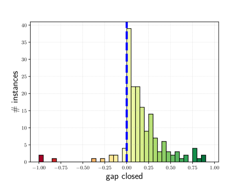
Figure 11: A bar diagram that visualizes the gap closed improvements for the $547$ selected instances. Each bar maps to an interval with width 0.05 that corresponds to the gap closed improvement. The height of the bar displays the total number of instances that achieved a value in the corresponding interval.

	# instances	gap closed
ALL	$547$	$7.5$%
>1% change	$178$	$20.8$%
>1% better	$165$	$24.9$%
>1% worse	$13$	$-31.1$%

Table 1: Aggregated results for the ROOTGAP experiments. The table shows the average gap closed values for different subsets of instances. ALL contains all instances, >1% better instances that improved by at least one percent, >1% worse instances that deteriorate by at least one percent, and >1% change is the union of instances in >1% better and >1% worse.

TREE experiment

For the TREE experiment, we use five permutations for each of the $564{}$ instances per setting in order to robustify the results against performance variability [30, 37]. A permutation of an instance randomly changes the order of the variables and the constraints. This can have a large impact on the behavior and the performance of a MINLP solver. An instance is considered to be solved by a setting if all permutations could be solved by this setting. Hence, if a setting solves more instances it means that it could consistently solve more instances over all permutations. For comparing solving times between different settings, we use the shifted geometric mean with a shift value of one second for the five permutations of an instance and then consider the shifted geometric mean of all these values.

Aggregated results for the tree experiments are shown in Table 2 and more detailed results for each instance are contained in Table LABEL:table:tree:detailed of the electronic supplement. SCIP with its default settings solves 244 of the 564 instances. When activating the use of projections for separation $3$ more instances are solved than with default SCIP; when activating it for both separation and propagation $5$ more instances are solved. Considering the total time, we see that on average SCIP+s and SCIP+s+p is $3\%$ faster than SCIP. The groups [1,tlim], [10,tlim], and [100,tlim] are the subsets of instances for which at least one setting solved the instance in more than one, ten, or $100$ seconds, respectively. These subsets form a hierarchy of increasingly difficult instance sets in an unbiased manner. Compared to SCIP, SCIP+s+p solves $4$ more instances on [1,tlim], $4$ more on [10,tlim], and $5$ more on [100,tlim]. With respect to time, SCIP+s+p is $11\%$ faster on [1,tlim], $18\%$ on [10,tlim], and even $36\%$ on [100,tlim] than SCIP.

A comparison of the second and the third column of Table 2 shows that both the separation and the propagation contribute to the larger number of solved instances. While activating separation alone does not improve the solving time, it can be seen that, more importantly, it does help to solve more instances in total.

		SCIP+s+p	SCIP+s		SCIP
	n	# solved	# solved	time	# solved	time
ALL	564	249	247	$+0\%{}$	244	$+3\%{}$
[1,tlim]	166	159	158	$+1\%{}$	155	$+1\%{}$
[10,tlim]	109	102	101	$+2\%{}$	98	$+18\%{}$
[100,tlim]	44	38	40	$-3\%{}$	33	$+36\%{}$

Table 2: Aggregated results of SCIP on the 564 potentially affected instances of the MINLPLib. For each instance, five permutation including the default permutation have been solved. An instance is considered to be solved when all permutations of this could be solved by a setting. Three different settings for SCIP are used: default settings SCIP, SCIP+s for activating separation, and SCIP+s+p for activating separation and propagation for bilinear terms that provide a useful two-dimensional projection. The column “time” reports the change of solving time relative to SCIP+s+p.

6 Conclusion

In this article, we presented techniques to improve the separation and propagation of bilinear terms when solving MINLPs with spatial branch-and-bound and gave an extensive computational study on a large heterogeneous test set. Our ideas are based on projecting a linear relaxation onto two variables that appear bilinearly by solving a sequence of LPs that are similar to the ones in OBBT. Instead of computing the full projection, we compute a relaxation of the projection that is described by few inequalities. By applying known polyhedral results, we are able to strengthen the separation of quadratic constraints by computing the convex and concave envelope of $x_{i}x_{j}$ on the two-dimensional projections. Additionally, we presented that the projections also enables us to tighten variable bounds. Computing the best possible bounds of $x_{i}$, $x_{j}$, and $x_{i}x_{j}$ on the projection is in general a nonconvex optimization problem. We proved that these problems can be efficiently solved by computing a discrete set of points. This allows us to efficiently solve these optimization problems at every node of the branch-and-bound tree.

Our experiments on the publicly available instances of the MINLPLib based on an implementation in the MINLP solver SCIP show that 564 of the 1682 instances provide nontrivial projections for at least one bilinear term. On these instances, it was possible to compute useful projections for 40.3% of all bilinear terms. When using the projection exhaustively during the separation of the root node, we observed an improvement of the achieved dual bounds on $165$ and a deterioration on only $13$ instances. The average gap closed improvement on all instances for which a change of at least one percent could be observed is $20.8$%. Finally, our tree experiments showed that the new techniques improve performance by $36$% on difficult instances and enable us to consistently solve more instances.

There are two interesting extensions of the presented methods. First, our propagation techniques do not only apply to polyhedral projections but also for general two-dimensional convex sets. How to compute these convex sets efficiently by using a convex relaxation of a MINLP remains an open question. Second, for models that contain symmetric structures the tightness of the two-dimensional projections and the performance improvements gained might profit particularly from symmetry-breaking constraints of the form $x_{i}\leq x_{j}$. These inequalities are in general not implied by a linear relaxation, but can be derived by considering formulation symmetry [34].

[Notes]

Table 3: Detailed results for the effectiveness of instances of the MINLPLib2 that contain bilinear terms. All instances for which Algorithm 1 has not been called are filtered out.

# LPs — total number of solved LPs
# iters — total number of LP iterations used
# filtered — total number of filtered candidates
time — time spent for solving all LPs (in seconds)
Instance	$\sum_{i,j}K_{ij}\phi_{ij}$	$\sum_{i,j}K_{ij}$	# LPs	# iters	# filtered	time
spar30-100-1	0	427	376	29724	878	0.69
spar30-100-2	0	430	493	43747	692	1.62
spar30-100-3	0	428	375	30584	912	0.71
spar30-60-1	0	250	178	10125	608	0.19
spar30-60-2	11	240	313	16239	260	0.60
spar30-60-3	0	288	410	22576	298	0.47
spar30-70-1	0	290	246	16683	600	0.51
spar30-70-2	0	288	376	22727	351	0.69
spar30-70-3	0	312	390	26509	445	0.89
spar30-80-1	0	343	248	18845	819	0.64
spar30-80-2	0	330	334	21244	584	0.79
spar30-80-3	0	349	599	42979	197	1.01
spar30-90-1	0	373	259	20843	927	0.68
spar30-90-2	0	391	455	36242	612	0.82
spar30-90-3	0	377	443	33980	557	0.77
genpool04	2	96	68	17445	124	0.51
genpool04i	2	48	72	16228	120	0.37
genpool04paper	2	96	78	22765	114	0.66
genpool10	0	600	358	131149	842	8.69
genpool10i	0	300	373	210402	827	17.02
genpool10paper	0	600	365	130411	835	8.71
genpool15	6	1350	706	151715	1994	5.28
genpool15i	1	675	858	1283245	1842	259.84
genpool15paper	6	1350	703	83492	1997	2.12
genpool20	2	2520	1275	342223	3765	18.79
genpool20i	2	1260	1375	2906822	3665	734.85
genpool20paper	2	2520	1272	369178	3768	18.44
mpss-basic-marvin-85-85	17	32	82	215187	46	84.02
mpss-basic-ob25-125-125	25	48	122	543425	70	421.12
mpss-basic-red-marvin-85-85	17	32	82	200911	46	61.60
mpss-basic-red-ob25-125-125	25	48	123	417319	69	257.45
mpss-extwarehouse-marvin-85-85	108	2414	1918	1170408	7738	735.45
mpss-extwarehouse-ob25-125-125	50	5428	1011	1308812	16928	2315.00
mpss-extwarehouse-red-ob25-125	34	5388	711	1003194	16628	1294.87
4stufen	13	35	86	2586	26	0.04
alkyl	4	9	24	167	10	0.00
alkylation	2	6	13	90	6	0.01
arki0003	0	360	57	232	25	0.19
arki0004	0	5200	2133	8072	6303	3.55
arki0005	672	3360	48	52935	28	25.00
arki0008	0	2299	583	422386	1305	226.68
arki0009	0	90	270	630	90	7.54
arki0010	0	45	135	315	45	1.53
arki0011	0	135	405	945	135	134.37
arki0012	0	135	405	945	135	173.27
arki0013	0	135	405	945	135	203.41
arki0014	0	135	405	945	135	161.04
arki0015	242	704	1634	835612	1182	831.92
arki0016	910	4634	12107	849097	3874	428.02
arki0017	562	4027	5383	343160	8636	127.38
arki0018	39	9804	10136	24930	19314	91.81
arki0019	494	1018	839	939037	1886	182.31
arki0020	5	2522	2518	6849376	4081	2412.48
arki0022	35	8302	83	1408754	6805	5769.45
arki0024	424	3452	2486	189804	1742	39.97
autocorr_bern35-35	0	595	176	16027	1758	2.84
batch0812_nc	16	37	45	1648	69	0.03
batch_nc	17	38	39	1757	79	0.06
bayes2_10	167	382	734	9412	794	0.21
bayes2_20	199	385	739	18121	801	0.36
bayes2_30	209	385	684	17985	856	0.38
bayes2_50	192	385	846	24357	694	0.35
bchoco05	9	15	31	472	16	0.02
bchoco06	10	21	40	692	26	0.02
bchoco07	19	30	58	3137	32	0.14
bchoco08	10	39	78	1966	39	0.11
beuster	7	62	74	4408	50	0.09
blend029	22	40	60	2318	52	0.06
blend146	76	168	163	14490	253	1.24
blend480	66	248	251	68194	357	3.81
blend531	84	204	209	14008	263	0.74
blend718	92	160	166	21204	234	1.04
blend721	64	168	162	20502	254	1.01
blend852	80	248	234	29613	374	1.96
btest14	0	114	19	220	277	0.02
camcns	59	282	517	233911	39	11.03
camshape100	101	296	268	6701	246	0.14
camshape200	201	596	528	21711	527	0.64
camshape400	398	1196	1044	77967	1094	1.82
camshape800	787	2396	2075	309133	2232	10.31
carton7	57	168	45	6177	31	0.19
carton9	75	207	61	3976	39	0.25
casctanks	52	267	337	16091	289	0.84
case_1scv2	147	1792	1614	1174876	1161	149.96
cesam2log	161	185	310	8280	357	0.64
chain100	99	99	101	102570	97	6.91
chain200	199	199	203	414072	196	26.95
chain400	399	399	406	2640373	392	425.25
chain50	49	49	51	12615	47	0.56
chem	10	20	39	565	1	0.01
chenery	8	22	40	815	32	0.02
chp_partload	572	1041	2515	1860625	595	575.41
chp_shorttermplan2b	0	960	310	72032	319	17.40
chp_shorttermplan2d	261	1632	351	83074	423	56.41
clay0203h	36	120	56	3141	21	0.10
clay0204h	52	160	79	7528	20	0.38
clay0205h	36	200	97	16328	28	0.96
clay0303h	0	180	52	1530	47	0.08
clay0304h	0	240	63	4337	59	0.26
clay0305h	0	300	87	7431	78	0.41
contvar	38	104	168	33084	81	2.31
crudeoil_lee1_05	45	48	107	6223	85	0.21
crudeoil_lee1_06	60	60	114	35898	126	2.22
crudeoil_lee1_07	72	72	133	28405	155	2.18
crudeoil_lee1_08	83	84	149	80563	187	3.84
crudeoil_lee1_09	95	96	169	50603	215	4.63
crudeoil_lee1_10	108	108	191	123973	241	13.94
crudeoil_lee2_05	94	106	232	93047	192	4.09
crudeoil_lee2_06	128	134	278	156948	258	15.09
crudeoil_lee2_07	157	162	353	313322	295	33.52
crudeoil_lee2_08	184	190	404	197679	356	18.43
crudeoil_lee2_09	212	218	444	210673	428	22.26
crudeoil_lee2_10	240	246	505	382964	479	45.80
crudeoil_lee3_05	165	212	446	177718	402	16.99
crudeoil_lee3_06	220	282	615	476446	513	44.64
crudeoil_lee3_07	272	352	804	424006	604	39.58
crudeoil_lee3_08	327	422	986	1145102	702	105.02
crudeoil_lee3_09	378	492	1149	1423496	819	244.22
crudeoil_lee3_10	431	562	1322	1369958	926	279.00
crudeoil_lee4_05	120	146	336	106502	248	7.57
crudeoil_lee4_06	145	184	405	242809	299	27.42
crudeoil_lee4_07	189	222	504	315668	384	52.81
crudeoil_lee4_08	231	260	606	555462	434	64.00
crudeoil_lee4_09	265	298	651	616486	541	134.83
crudeoil_lee4_10	296	336	739	890562	605	210.96
crudeoil_li01	39	56	146	18677	78	0.73
crudeoil_li02	0	15	54	50677	6	4.42
crudeoil_li03	59	192	405	227910	363	22.54
crudeoil_li05	58	192	413	259797	355	18.41
crudeoil_li06	39	192	391	160716	377	18.05
crudeoil_li11	47	192	390	225903	378	25.07
crudeoil_li21	50	192	360	332054	408	44.15
crudeoil_pooling_ct1	9	64	135	17690	65	0.54
crudeoil_pooling_ct2	0	70	149	13541	131	0.62
crudeoil_pooling_ct3	12	223	324	159213	485	9.49
crudeoil_pooling_ct4	0	95	164	26917	216	1.80
crudeoil_pooling_dt1	10	570	1415	3316265	865	710.29
crudeoil_pooling_dt2	215	1106	2277	5868404	2147	2682.20
crudeoil_pooling_dt3	12	2707	3942	5403108	6886	3948.09
crudeoil_pooling_dt4	147	1121	2221	6070617	2263	1746.77
csched1	5	7	17	274	11	0.00
csched1a	0	7	13	347	4	0.00
csched2	16	57	102	24762	126	0.34
csched2a	24	57	78	5105	67	0.25
deb6	62	88	118	6152	58	1.35
deb7	62	176	116	5958	60	1.18
deb8	52	176	122	10403	54	1.62
deb9	62	176	116	5958	60	1.18
dispatch	0	3	12	62	0	0.00
edgecross10-060	0	982	20	2679	69	0.38
edgecross14-039	0	625	67	2645	454	0.56
elec100	0	14850	12235	985544	44955	575.46
elec25	0	900	824	21707	2586	2.86
elec50	0	3675	3529	182404	10608	45.22
elf	3	3	8	328	4	0.02
eq6_1	0	92	74	1396	136	0.05
etamac	0	9	24	392	12	0.03
ethanolh	1	4	11	239	1	0.00
ethanolm	1	4	7	183	5	0.01
ex1226	1	1	1	7	1	0.00
ex1233	0	12	7	190	21	0.01
ex1243	0	12	16	618	13	0.03
ex1244	0	17	24	1038	19	0.02
ex1252	5	15	30	284	30	0.02
ex1252a	7	15	27	330	33	0.01
ex1263	0	16	20	2947	12	0.07
ex1263a	3	16	24	457	8	0.00
ex1264	1	16	16	1204	30	0.02
ex1264a	0	16	22	633	16	0.01
ex1265	2	25	33	2550	22	0.04
ex1265a	3	25	31	1230	21	0.02
ex1266	0	36	36	1859	70	0.03
ex14_1_2	6	23	11	177	5	0.00
ex14_1_3	2	2	3	14	1	0.00
ex14_1_6	0	10	3	31	9	0.00
ex14_1_8	4	10	14	149	6	0.00
ex2_1_9	22	22	22	301	43	0.01
ex3_1_1	4	5	9	65	3	0.00
ex3_1_2	9	9	15	120	1	0.00
ex3_1_4	2	3	3	16	5	0.00
ex5_2_2_case1	4	4	6	37	2	0.00
ex5_2_2_case2	4	4	6	68	2	0.01
ex5_2_2_case3	4	4	6	38	2	0.00
ex5_2_4	4	14	8	99	9	0.00
ex5_2_5	9	195	29	544	171	0.00
ex5_3_2	12	12	28	255	20	0.01
ex5_3_3	32	103	105	1352	175	0.04
ex5_4_2	4	5	9	80	3	0.00
ex5_4_3	7	10	22	250	6	0.01
ex5_4_4	1	18	30	320	24	0.00
ex6_1_1	2	18	30	266	25	0.00
ex6_1_2	4	7	15	88	3	0.00
ex6_1_3	3	39	63	475	51	0.03
ex6_1_4	0	15	28	362	8	0.02
ex6_2_10	15	51	95	1886	46	0.06
ex6_2_11	8	24	45	686	10	0.01
ex6_2_12	6	26	50	744	22	0.02
ex6_2_13	8	37	69	1468	34	0.02
ex6_2_14	11	34	63	703	31	0.03
ex6_2_5	12	30	34	590	35	0.02
ex6_2_6	12	12	24	261	0	0.01
ex6_2_7	3	27	42	2409	20	0.03
ex6_2_8	9	9	18	172	0	0.00
ex6_2_9	10	34	62	1415	32	0.03
ex7_2_1	2	11	13	255	7	0.01
ex7_2_2	4	4	13	106	3	0.00
ex7_2_3	0	4	4	44	7	0.00
ex7_2_4	5	10	16	304	8	0.01
ex7_3_1	0	11	22	95	7	0.01
ex7_3_2	0	2	1	0	0	0.00
ex7_3_3	0	3	8	24	0	0.00
ex7_3_4	0	13	20	76	0	0.00
ex7_3_5	0	20	7	21	2	0.00
ex8_1_1	1	2	3	23	1	0.00
ex8_1_7	0	1	2	26	2	0.01
ex8_2_1b	0	50	100	1889	0	0.04
ex8_2_2b	0	6156	8721	284173	5629	33.43
ex8_2_3b	1	9065	10878	317649	7252	31.03
ex8_2_4b	1	106	212	4847	18	0.16
ex8_2_5b	0	12312	18468	966240	9681	83.38
ex8_3_1	0	229	221	1721	535	0.09
ex8_3_11	0	229	226	1916	530	0.07
ex8_3_12	0	244	204	3000	492	0.08
ex8_3_13	0	214	214	1783	482	0.08
ex8_3_14	0	214	208	6532	468	0.28
ex8_3_2	0	214	203	1175	513	0.05
ex8_3_3	0	214	202	1807	514	0.05
ex8_3_4	0	214	204	1748	512	0.08
ex8_3_5	0	214	212	2200	504	0.10
ex8_3_7	0	271	280	1435	622	0.08
ex8_3_8	3	269	257	2548	639	0.12
ex8_3_9	0	107	121	2092	247	0.07
ex8_4_1	10	10	40	1067	0	0.04
ex8_4_2	8	30	62	3235	58	0.09
ex8_4_4	10	12	41	1518	7	0.03
ex8_4_5	14	22	14	164	2	0.00
ex8_4_6	0	32	56	120	56	0.01
ex8_4_7	0	50	98	5689	22	0.11
ex8_4_8_bnd	10	20	29	5894	15	0.12
ex8_5_1	3	12	8	12	26	0.01
ex8_5_2	0	8	2	0	0	0.00
ex8_5_5	0	6	1	0	1	0.00
ex8_6_1	0	85	85	107	255	0.02
ex8_6_2	0	85	93	2937	247	0.08
ex9_1_2	0	4	5	0	3	0.00
ex9_2_2	1	2	5	11	3	0.00
ex9_2_3	6	6	16	89	8	0.01
ex9_2_4	2	2	8	57	0	0.01
ex9_2_5	0	3	3	0	3	0.00
ex9_2_6	4	6	9	49	15	0.00
ex9_2_7	0	4	12	67	4	0.00
fdesign10	0	1	1	61	2	0.01
fdesign25	0	1	1	137	2	0.00
feedtray	89	259	617	36384	99	2.26
filter	0	3	5	41	3	0.01
fin2bb	21	61	163	90885	1	5.72
forest	27	90	203	7570	157	0.17
gabriel01	102	336	333	49167	499	3.23
gabriel02	220	672	685	172756	979	23.59
gabriel04	234	992	909	366261	1523	46.82
gabriel05	468	1704	1746	342590	2382	79.47
gabriel06	1301	6112	6459	4493136	8261	3371.62
gabriel07	1638	7640	7541	4339658	10859	3372.07
gabriel09	914	5688	4392	1762991	7992	1425.87
gams02	174	192	530	64798	238	2.19
gams03	47	53040	528	307254	150694	561.69
gancns	5	214	181	11647	129	0.72
gasnet	14	41	58	3054	66	0.11
gasnet_al1	10	145	57	1348	31	0.29
gasnet_al2	10	145	56	1333	32	0.15
gasnet_al3	10	145	57	1210	31	0.16
gasnet_al4	10	145	57	1406	31	0.20
gasnet_al5	10	145	56	1217	32	0.21
gasprod_sarawak01	3	34	88	7159	48	0.13
gasprod_sarawak16	169	544	1514	470279	662	46.80
gasprod_sarawak81	846	2754	7094	5117307	3922	1523.17
gastrans135	105	228	498	22679	169	3.98
gastrans582_cold13	114	221	257	11320	71	1.76
gastrans582_cold13_95	114	221	255	11686	73	1.80
gastrans582_cold17	120	222	289	11293	80	1.41
gastrans582_cold17_95	120	222	293	10928	76	1.25
gastrans582_cool12	120	221	277	13251	86	2.21
gastrans582_cool12_95	111	221	277	9241	86	2.16
gastrans582_cool14	111	220	278	10874	78	2.15
gastrans582_cool14_95	111	220	283	8321	73	1.80
gastrans582_freezing27	120	221	310	11716	65	2.69
gastrans582_freezing27_95	120	221	307	11652	68	1.57
gastrans582_freezing30	120	221	317	13436	66	3.20
gastrans582_freezing30_95	120	221	322	10444	61	1.88
gastrans582_mild10	111	219	269	8309	69	1.38
gastrans582_mild10_95	112	219	271	7451	68	1.55
gastrans582_mild11	112	220	266	12155	78	1.40
gastrans582_mild11_95	111	220	269	12152	75	1.27
gastrans582_warm15	115	222	264	10302	66	1.13
gastrans582_warm15_95	115	222	260	11044	70	2.02
gastrans582_warm31	114	224	255	10034	81	1.38
gastrans582_warm31_95	114	224	266	9873	71	1.60
genpooling_lee1	30	72	41	2765	55	0.06
genpooling_lee2	45	108	56	5544	88	0.12
genpooling_meyer04	0	96	69	17739	123	0.43
genpooling_meyer10	4	600	376	211058	824	17.09
genpooling_meyer15	0	1350	740	942004	1960	123.95
ghg_1veh	47	63	47	2601	24	0.06
ghg_2veh	3	148	101	4668	63	0.12
ghg_3veh	97	255	263	22022	41	0.95
glider100	0	1102	201	0	506	0.01
glider200	0	2202	401	0	1006	0.04
glider400	0	4402	801	0	2006	0.17
glider50	0	552	101	0	256	0.00
gsg_0001	18	20	80	2304	0	0.05
haverly	0	4	3	0	1	0.00
heatexch_gen1	4	72	77	2480	99	0.08
heatexch_gen2	0	67	70	3032	98	0.17
heatexch_gen3	6	420	373	120388	667	4.88
heatexch_spec1	0	12	8	232	17	0.02
heatexch_spec2	0	16	11	865	25	0.07
heatexch_spec3	0	60	25	5168	114	0.32
heatexch_trigen	0	18	41	650	31	0.03
hhfair	0	9	6	0	9	0.00
himmel11	9	9	24	212	2	0.00
himmel16	0	7	20	345	8	0.03
house	0	5	7	0	0	0.00
hs62	0	6	4	19	11	0.00
hvb11	0	32	60	9550	4	0.32
hybriddynamic_fixedcc	0	20	14	55	31	0.01
hybriddynamic_var	7	13	22	413	6	0.01
hybriddynamic_varcc	0	68	20	41	126	0.00
hydroenergy1	40	69	179	15287	97	0.75
hydroenergy2	42	161	364	100952	280	4.51
hydroenergy3	66	299	713	244963	483	19.74
infeas1	1148	1237	295	119888	121	9.50
kall_circles_c6a	16	43	75	1647	57	0.03
kall_circles_c6b	16	43	69	1158	76	0.02
kall_circles_c6c	16	57	96	2667	80	0.07
kall_circles_c7a	23	57	78	1742	102	0.04
kall_circles_c8a	36	73	110	3036	110	0.05
kall_circlespolygons_c1p12	3	19	36	958	40	0.01
kall_circlespolygons_c1p13	3	19	47	855	29	0.01
kall_circlespolygons_c1p5a	4	101	217	4966	187	0.25
kall_circlespolygons_c1p5b	10	611	1242	40167	1202	4.18
kall_circlespolygons_c1p6a	11	877	1778	166686	1730	27.74
kall_circlesrectangles_c1r11	3	21	36	722	48	0.01
kall_circlesrectangles_c1r12	3	21	38	666	46	0.01
kall_circlesrectangles_c1r13	3	21	41	549	43	0.02
kall_circlesrectangles_c6r1	9	141	264	7512	281	0.38
kall_circlesrectangles_c6r29	23	283	596	35029	515	2.22
kall_circlesrectangles_c6r39	30	457	967	49535	843	5.73
kall_congruentcircles_c31	4	7	16	151	6	0.00
kall_congruentcircles_c32	4	7	10	65	17	0.00
kall_congruentcircles_c41	6	6	11	104	2	0.00
kall_congruentcircles_c42	7	13	26	273	21	0.02
kall_congruentcircles_c51	11	21	43	612	31	0.06
kall_congruentcircles_c52	11	21	35	402	47	0.03
kall_congruentcircles_c61	16	31	63	1342	46	0.08
kall_congruentcircles_c62	16	31	41	515	80	0.04
kall_congruentcircles_c63	16	31	43	1014	51	0.03
kall_congruentcircles_c71	22	43	87	2185	64	0.03
kall_congruentcircles_c72	22	43	80	876	71	0.02
kall_diffcircles_10	2	81	88	1749	156	0.04
kall_diffcircles_5a	5	21	33	490	31	0.01
kall_diffcircles_5b	1	21	32	749	32	0.02
kall_diffcircles_6	1	31	45	553	47	0.01
kall_diffcircles_7	2	43	45	1376	91	0.03
kall_diffcircles_8	1	49	84	1145	65	0.03
kall_diffcircles_9	2	64	88	1915	87	0.04
kall_ellipsoids_tc02b	0	48	66	1608	108	0.07
kall_ellipsoids_tc03c	0	108	134	3649	245	0.22
kall_ellipsoids_tc05a	57	960	1569	240891	591	54.45
kissing2	0	73768	12356	309820	113138	154.96
knp3-12	0	198	120	3307	550	0.10
knp4-24	0	1104	765	55857	2823	5.95
knp5-40	0	3900	3609	415492	9024	59.93
knp5-41	0	4100	2287	239255	10872	74.57
knp5-42	0	4305	2718	366533	11148	36.76
knp5-43	0	4515	3549	622735	10778	66.26
knp5-44	0	4730	3007	499275	12199	89.59
korcns	23	48	93	7331	43	0.21
launch	2	15	41	650	12	0.01
least	0	12	4	0	6	0.00
lnts100	0	796	313	566	515	0.27
lnts200	0	1596	613	1166	1015	2.14
lnts400	0	3196	1213	2366	2015	9.34
lnts50	0	396	163	266	265	0.10
mathopt1	2	2	4	28	2	0.00
mathopt4	1	2	4	35	0	0.00
mathopt5_3	0	2	4	29	2	0.00
mathopt5_6	0	1	2	4	0	0.00
maxmin	0	132	158	23362	222	0.55
maxmineig2	0	294	354	716	822	0.12
milinfract	0	1	2	28	0	0.07
minlphi	0	4	4	15	4	0.00
minlphix	0	8	4	24	7	0.01
multiplants_mtg1a	49	76	117	20616	20	0.94
multiplants_mtg1b	50	71	105	23828	28	0.97
multiplants_mtg1c	46	76	105	45487	35	2.09
multiplants_mtg2	58	101	158	28179	20	1.56
multiplants_mtg5	93	125	156	10902	26	0.34
multiplants_mtg6	121	173	222	35782	22	1.44
multiplants_stg1	1	67	186	68380	82	2.35
multiplants_stg1a	1	49	104	41238	92	1.48
multiplants_stg1b	1	55	171	77258	49	2.87
multiplants_stg1c	1	43	80	26555	92	0.94
multiplants_stg5	1	49	162	63104	34	1.38
multiplants_stg6	1	65	197	112837	63	4.47
ndcc12	528	528	1056	349712	492	15.61
ndcc12persp	43	124	49	39797	80	2.23
ndcc13	535	546	1092	326759	390	18.66
ndcc13persp	31	112	70	52843	43	4.13
ndcc14	756	756	1512	505373	742	34.80
ndcc14persp	49	156	73	62300	85	4.04
ndcc15	538	540	1080	296086	465	22.86
ndcc15persp	35	104	65	32859	36	2.52
ndcc16	960	960	1920	928823	960	65.00
ndcc16persp	57	180	93	90509	85	10.33
ngone	0	195	147	21301	485	6.99
nous1	20	58	63	502	133	0.02
nous2	20	58	80	717	116	0.03
nuclear10a	852	22962	226	4745248	1590	1362.17
nuclear14a	1905	2568	1108	2219487	428	227.05
nuclear14b	1449	1992	1082	1529710	454	288.17
nuclear25a	2058	2720	1131	1776885	469	201.09
nuclear25b	1624	2095	1328	2504727	272	424.74
nuclear49a	4788	7275	2820	22111293	708	5512.67
nuclear49b	3867	4874	2957	11491979	571	3982.06
nuclearvb	0	1036	14	0	154	0.00
nuclearvc	0	1036	14	0	154	0.00
nuclearvd	0	1474	14	0	154	0.00
nuclearve	0	1474	14	0	154	0.00
nuclearvf	0	1474	14	0	154	0.00
nvs01	1	2	3	24	1	0.00
nvs02	1	9	10	177	18	0.00
nvs04	0	2	2	25	2	0.00
nvs05	1	9	19	377	8	0.02
nvs06	0	2	2	6	4	0.00
nvs13	44	49	16	207	23	0.01
nvs14	1	9	10	175	18	0.00
nvs15	0	2	2	6	0	0.00
nvs16	0	7	6	62	11	0.00
nvs17	140	140	62	1486	20	0.01
nvs18	64	87	20	316	39	0.01
nvs19	206	206	78	3635	34	0.05
nvs20	10	30	60	2095	9	0.08
nvs21	0	2	3	5	3	0.00
nvs22	0	10	20	275	12	0.02
nvs23	290	290	109	4244	35	0.06
nvs24	399	399	128	6503	52	0.10
oil	77	331	688	133697	80	13.16
oil2	80	270	596	6846	8	2.27
ortez	5	24	58	861	18	0.03
orth_d3m6	8	46	42	255	78	0.01
orth_d3m6_pl	15	225	240	939	460	0.22
orth_d4m6_pl	6	105	295	1352	125	0.09
otpop	11	12	48	2050	0	0.06
parallel	65	110	120	12835	137	0.38
pindyck	31	32	99	9237	29	0.37
pointpack04	7	12	14	150	24	0.01
pointpack06	16	30	34	538	72	0.02
pointpack08	29	56	51	688	147	0.02
pointpack10	46	90	97	1858	221	0.09
pointpack12	67	132	159	3731	299	0.13
pointpack14	92	182	239	6939	369	0.45
pollut	3	20	29	281	16	0.01
pooling_adhya1pq	5	20	16	286	64	0.01
pooling_adhya1stp	2	40	40	704	120	0.01
pooling_adhya1tp	2	20	35	520	45	0.01
pooling_adhya2pq	1	20	22	81	58	0.00
pooling_adhya2stp	0	40	51	415	109	0.01
pooling_adhya2tp	2	20	28	252	52	0.01
pooling_adhya3pq	1	32	36	184	92	0.01
pooling_adhya3stp	0	64	71	473	185	0.03
pooling_adhya3tp	6	32	59	808	69	0.02
pooling_adhya4pq	1	40	42	428	118	0.01
pooling_adhya4stp	0	80	80	865	240	0.03
pooling_adhya4tp	6	40	79	731	81	0.03
pooling_bental4pq	6	6	17	109	7	0.01
pooling_bental4stp	0	12	21	158	27	0.01
pooling_bental4tp	6	6	14	111	10	0.00
pooling_bental5stp	0	120	122	796	358	0.04
pooling_digabel16	27	432	197	6667	379	0.18
pooling_digabel18	261	1080	680	58487	760	2.57
pooling_digabel19	159	636	436	42436	412	1.03
pooling_epa1	120	142	153	17238	71	0.53
pooling_epa2	292	351	293	50899	151	2.99
pooling_epa3	252	1480	967	411230	673	96.18
pooling_foulds2stp	0	32	32	139	96	0.00
pooling_foulds3stp	0	1024	1006	9068	3090	0.93
pooling_foulds4stp	0	1024	1006	20704	3090	1.26
pooling_foulds5stp	2	1024	993	30287	3103	2.66
pooling_haverly1pq	4	4	8	56	8	0.00
pooling_haverly1stp	4	8	24	150	8	0.00
pooling_haverly1tp	4	4	12	86	4	0.00
pooling_haverly2pq	4	4	14	106	2	0.00
pooling_haverly2stp	4	8	20	138	12	0.01
pooling_haverly2tp	4	4	10	72	6	0.01
pooling_haverly3pq	4	4	12	127	4	0.00
pooling_haverly3stp	6	8	24	247	8	0.01
pooling_haverly3tp	4	4	12	87	4	0.01
pooling_rt2pq	1	18	27	175	45	0.00
pooling_rt2stp	10	36	56	1416	88	0.02
pooling_rt2tp	10	18	34	833	38	0.01
pooling_sppa0pq	6	329	413	61146	903	3.23
pooling_sppa0stp	2	658	803	177185	1829	7.43
pooling_sppa0tp	8	329	442	147332	874	6.07
pooling_sppa5pq	9	968	968	204838	2904	14.61
pooling_sppa5stp	4	1936	2030	397767	5714	28.79
pooling_sppa5tp	16	968	1007	290852	2865	13.58
pooling_sppa9pq	8	1828	1851	115410	5461	10.06
pooling_sppa9stp	2	3820	3880	417686	11400	35.28
pooling_sppa9tp	9	1992	2153	111430	5815	9.78
pooling_sppb0pq	14	1153	1176	209657	3436	31.45
pooling_sppb0stp	2	2306	2745	496741	6479	94.31
pooling_sppb0tp	18	1153	1429	482396	3183	39.62
pooling_sppb2pq	17	3093	3161	1133060	9211	262.35
pooling_sppb2stp	2	6186	6342	4395622	18402	1047.31
pooling_sppb2tp	16	3093	3723	1372710	8649	145.49
pooling_sppb5pq	16	7947	8215	11130274	23573	1572.60
pooling_sppb5stp	36	15894	15290	25499298	47718	6806.60
pooling_sppc0pq	35	2826	2925	4783872	8379	1451.83
pooling_sppc0stp	15	5652	5693	10640160	16915	4767.84
pooling_sppc0tp	27	2826	3958	5526943	7346	1774.29
pooling_sppc1pq	25	4770	5557	13864945	13523	4173.37
pooling_sppc1stp	50	9540	5206	15821587	28614	6955.07
pooling_sppc1tp	43	4770	6021	14955663	13059	4526.10
pooling_sppc3pq	26	9116	1947	9173015	26745	6385.09
pooling_sppc3stp	5	18232	858	10582833	53501	4778.78
pooling_sppc3tp	13	9116	714	9725129	25461	4958.52
powerflow0009r	22	116	44	1314	92	0.04
powerflow0014r	48	264	162	11311	142	0.32
powerflow0030r	192	584	391	80692	249	4.58
powerflow0039r	192	700	290	100404	438	6.71
powerflow0057r	166	1088	508	43675	708	3.25
powerflow0118r	276	2748	1116	175707	1700	28.98
powerflow0300r	978	6020	2778	2390185	3742	893.46
primary	2879	2917	1731	65916	2097	2.68
prob07	0	30	6	0	14	0.00
prob09	1	1	3	56	1	0.00
process	0	3	9	104	2	0.01
procurement1large	68	136	79	211	198	1.83
procurement1mot	12	24	23	423	37	0.03
prolog	0	8	4	0	4	0.00
qp3	50	50	50	850	82	0.02
rbrock	1	1	2	17	0	0.00
ringpack_10_1	50	660	104	4242	255	0.13
ringpack_10_2	60	840	106	2041	252	0.09
ringpack_20_1	712	4674	405	22259	1092	1.19
ringpack_20_2	782	5434	426	64877	1076	2.59
ringpack_20_3	0	6110	429	35598	1066	1.29
ringpack_30_1	2672	14866	1097	156015	2356	9.75
ringpack_30_2	2856	16606	898	96546	2548	6.66
robot100	0	1489	594	1485	594	0.89
robot200	0	2989	1194	2985	1194	4.23
robot400	0	5989	2394	5985	2394	24.30
robot50	0	739	294	735	294	0.15
rocket100	0	995	299	5150	897	0.13
rocket200	0	1995	599	20302	1797	0.97
rocket400	0	3995	1199	80604	3597	4.17
rocket50	0	495	149	1325	447	0.02
rsyn0805h	1	9	9	117	10	0.01
rsyn0805m02h	1	18	21	370	17	0.04
rsyn0805m03h	4	27	32	1049	24	0.07
rsyn0805m04h	4	36	42	1746	28	0.21
rsyn0810h	2	18	16	240	17	0.01
rsyn0810m02h	0	36	35	880	36	0.06
rsyn0810m03h	5	54	51	1502	56	0.23
rsyn0810m04h	8	72	75	3184	61	0.33
rsyn0815h	0	33	29	910	27	0.03
rsyn0815m02h	1	66	59	2346	54	0.12
rsyn0815m03h	5	99	91	6038	81	0.58
rsyn0815m04h	7	132	123	10680	102	0.91
rsyn0820h	0	42	41	810	33	0.05
rsyn0820m02h	1	84	71	2896	79	0.26
rsyn0820m03h	3	126	111	7518	117	1.04
rsyn0820m04h	5	168	147	11909	159	1.81
rsyn0830h	1	60	46	640	73	0.05
rsyn0830m02h	0	120	108	3897	110	0.32
rsyn0830m03h	0	180	159	8164	166	1.08
rsyn0830m04h	1	239	204	11142	229	1.26
rsyn0840h	1	84	64	1314	98	0.18
rsyn0840m02h	4	168	153	4281	145	0.99
rsyn0840m03h	1	252	219	13505	234	2.26
rsyn0840m04h	8	335	307	28075	281	6.40
saa_2	5424	8992	7386	958322	254	634.91
sep1	2	6	24	216	0	0.01
sepasequ_complex	70	611	643	51204	799	7.13
sepasequ_convent	192	1046	1144	110380	794	8.26
sfacloc1_2_95	2	14	49	2259	7	0.06
sfacloc1_3_95	3	21	62	2242	22	0.06
sfacloc1_4_95	0	28	81	2321	31	0.14
sjup2	0	44400	2836	0	80478	0.04
smallinvSNPr1b010-011	541	4950	6853	288946	7964	11.35
smallinvSNPr1b020-022	772	4950	6678	461149	8138	17.51
smallinvSNPr1b050-055	1183	4950	4827	304980	10007	6.60
smallinvSNPr1b100-110	649	4950	6483	521834	8331	11.54
smallinvSNPr1b150-165	647	4950	6493	456477	8320	10.18
smallinvSNPr1b200-220	634	4950	6590	599430	8222	20.05
smallinvSNPr2b010-011	358	4950	7255	396469	7560	15.99
smallinvSNPr2b020-022	1249	4950	6577	393384	8238	9.65
smallinvSNPr2b050-055	716	4950	4984	270082	9851	8.58
smallinvSNPr2b100-110	562	4950	6943	391858	7869	19.52
smallinvSNPr2b150-165	882	4950	6765	396274	8054	15.25
smallinvSNPr2b200-220	1545	4950	6762	585985	8055	12.92
smallinvSNPr3b010-011	360	4950	7737	386626	7077	14.93
smallinvSNPr3b020-022	450	4950	7342	390364	7471	14.49
smallinvSNPr3b050-055	406	4950	3577	233254	11266	12.21
smallinvSNPr3b100-110	1136	4950	4886	286460	9952	6.59
smallinvSNPr3b150-165	585	4950	7335	524362	7477	21.95
smallinvSNPr3b200-220	875	4950	4575	244438	10259	10.09
smallinvSNPr4b010-011	433	4950	8298	625317	6508	19.41
smallinvSNPr4b020-022	1097	4950	5470	222705	9385	8.40
smallinvSNPr4b050-055	1039	4950	3741	213594	11107	4.69
smallinvSNPr4b100-110	851	4950	4119	288191	10720	6.06
smallinvSNPr4b150-165	629	4950	4201	334772	10636	7.07
smallinvSNPr4b200-220	860	4950	4324	193061	10511	7.40
smallinvSNPr5b010-011	378	4950	8319	492164	6488	14.18
smallinvSNPr5b020-022	595	4950	8319	477858	6486	13.18
smallinvSNPr5b050-055	1004	4950	5163	297039	9676	12.19
smallinvSNPr5b100-110	999	4950	4972	246117	9866	8.84
smallinvSNPr5b150-165	967	4950	4783	225261	10057	5.27
smallinvSNPr5b200-220	966	4950	4617	248387	10220	9.68
space25	0	86	12	225	20	0.00
space25a	0	86	24	658	32	0.02
space960	12	3740	2365	7577269	9330	6504.43
spectra2	1040	1080	354	32394	186	1.60
sporttournament14	0	168	80	2589	222	0.23
spring	3	3	10	142	0	0.00
sssd08-04	0	12	4	261	4	0.00
sssd08-04persp	12	36	24	734	12	0.03
sssd12-05	0	15	5	415	5	0.01
sssd12-05persp	15	45	30	1347	15	0.05
sssd15-04	0	12	4	170	4	0.00
sssd15-04persp	12	36	24	1165	12	0.05
sssd15-06	0	18	6	655	6	0.02
sssd15-06persp	18	54	36	1758	18	0.06
sssd15-08	0	24	8	1045	8	0.02
sssd15-08persp	24	72	48	3258	24	0.16
sssd16-07	0	21	7	617	7	0.02
sssd16-07persp	21	63	42	2037	21	0.10
sssd18-06	0	18	6	905	6	0.03
sssd18-06persp	16	54	34	3788	18	0.13
sssd18-08	0	24	8	1077	8	0.04
sssd18-08persp	24	72	48	7449	24	0.16
sssd20-04	0	12	4	309	4	0.01
sssd20-04persp	12	36	24	1056	12	0.02
sssd20-08	0	24	8	1211	8	0.03
sssd20-08persp	24	72	48	3969	24	0.18
sssd22-08	0	24	8	1186	8	0.05
sssd22-08persp	24	72	48	6662	24	0.31
sssd25-04	0	12	4	214	4	0.01
sssd25-04persp	12	36	24	2117	12	0.05
sssd25-08	0	24	8	647	8	0.03
sssd25-08persp	24	72	48	3496	24	0.10
st_bpaf1a	3	5	9	57	3	0.00
st_e03	5	5	11	170	1	0.01
st_e04	1	1	1	11	1	0.00
st_e05	2	2	7	38	1	0.00
st_e07	4	4	4	35	4	0.00
st_e08	1	1	2	8	0	0.00
st_e09	2	2	4	18	0	0.00
st_e11	1	1	4	18	0	0.00
st_e16	10	10	26	491	2	0.01
st_e17	0	1	2	8	0	0.00
st_e23	1	1	2	10	0	0.00
st_e25	4	6	12	77	1	0.00
st_e28	9	9	24	212	2	0.01
st_e30	2	6	17	211	7	0.01
st_e31	2	6	9	108	15	0.00
st_e32	308	314	413	25878	230	0.66
st_e33	0	4	4	24	4	0.00
st_e35	0	19	20	108	6	0.01
st_e36	3	3	3	31	1	0.00
st_e38	2	4	6	55	3	0.00
st_e40	1	3	4	29	8	0.01
st_e41	14	14	24	285	4	0.01
st_e42	0	1	3	0	1	0.00
st_glmp_fp1	0	1	2	8	0	0.00
st_glmp_fp2	0	1	2	9	0	0.00
st_glmp_fp3	1	1	2	8	0	0.00
st_glmp_kk90	0	1	2	11	0	0.00
st_glmp_kk92	1	1	2	11	0	0.00
st_glmp_kky	2	2	4	24	0	0.00
st_glmp_ss1	1	1	2	11	0	0.00
st_glmp_ss2	1	1	2	10	0	0.00
st_iqpbk1	26	28	53	3135	9	0.06
st_iqpbk2	28	28	52	2565	9	0.06
st_jcbpaf2	3	5	9	137	3	0.00
st_qpc-m1	10	10	13	112	7	0.00
st_qpc-m3a	45	45	46	863	110	0.02
st_qpc-m3b	45	45	45	1079	72	0.03
st_qpk1	1	1	2	10	1	0.00
st_robot	1	5	5	45	7	0.01
steenbrf	0	72	36	0	68	0.00
super3t	193	483	1241	364974	395	35.29
syn05h	0	9	10	73	9	0.00
syn05m02h	0	18	20	238	17	0.01
syn05m03h	0	27	28	345	30	0.02
syn05m04h	0	36	35	524	44	0.02
syn10h	0	18	15	125	18	0.00
syn10m02h	0	36	28	441	40	0.02
syn10m03h	0	54	42	880	64	0.03
syn10m04h	0	72	56	1298	86	0.05
syn15h	0	33	27	420	32	0.02
syn15m02h	0	66	52	1135	66	0.04
syn15m03h	0	99	75	2006	107	0.13
syn15m04h	0	132	110	4722	124	0.35
syn20h	0	42	35	499	43	0.02
syn20m02h	0	84	73	2120	82	0.15
syn20m03h	0	126	99	3920	137	0.25
syn20m04h	0	168	131	5471	183	0.31
syn30h	0	60	52	653	58	0.04
syn30m02h	0	120	102	3874	118	0.39
syn30m03h	0	180	157	9203	176	0.62
syn30m04h	0	239	205	13332	223	1.58
syn40h	0	84	70	1141	81	0.10
syn40m02h	0	168	146	6402	157	0.72
syn40m03h	0	252	211	13533	244	1.17
syn40m04h	0	335	313	37671	281	2.74
synheat	0	12	7	171	18	0.01
tanksize	11	36	44	1066	0	0.03
tln12	0	144	118	28891	337	1.13
tln4	12	16	18	622	21	0.01
tln5	25	25	25	1666	34	0.04
tln6	0	36	31	2491	79	0.06
tln7	0	49	43	3542	122	0.08
tls12	0	252	28	8908	35	1.64
tls2	1	4	3	72	2	0.00
tls4	0	25	12	842	8	0.03
tls5	0	72	9	1000	11	0.03
tls6	0	91	14	1909	6	0.08
tls7	0	49	64	13676	45	1.09
tltr	2	27	18	1915	23	0.05
torsion100	0	19700	512	5967479	27014	3603.99
torsion25	0	4850	2736	2430701	6964	525.13
torsion50	0	9800	5852	12862528	13748	6125.10
torsion75	0	14750	678	6370943	19954	4492.02
transswitch0009r	14	140	83	3931	53	0.13
transswitch0014r	0	344	71	1905	233	0.13
transswitch0030r	12	736	268	13058	372	1.43
transswitch0039r	2	872	257	9100	467	1.76
transswitch0057r	12	1396	702	86215	514	29.72
transswitch0118r	16	3452	1785	406369	1027	254.48
transswitch0300r	324	7492	3752	390991	2764	897.23
tricp	0	462	272	19337	870	0.57
uselinear	0	5570	4526	1047666	12239	70.06
util	5	5	19	330	1	0.01
var_con10	112	240	322	10126	158	1.50
var_con5	108	240	324	6706	156	1.34
wager	2	114	63	2309	30	0.11
waste	5	1230	77	8385	187	0.21
wastepaper3	0	54	10	379	14	0.02
wastepaper4	0	88	9	268	23	0.01
wastepaper5	0	130	9	216	31	0.01
wastepaper6	0	180	10	343	38	0.01
wastewater02m1	6	8	17	87	12	0.02
wastewater02m2	9	12	48	836	0	0.04
wastewater04m1	12	16	24	186	36	0.00
wastewater04m2	6	18	68	1154	4	0.03
wastewater05m1	0	45	42	537	129	0.01
wastewater05m2	0	48	88	3589	104	0.22
wastewater11m1	24	63	115	5498	130	0.07
wastewater11m2	0	112	202	19060	246	0.20
wastewater12m1	55	120	223	8320	247	0.18
wastewater12m2	3	220	520	67647	360	1.35
wastewater13m1	64	255	484	13676	521	0.24
wastewater13m2	0	480	746	153382	1174	3.14
wastewater14m1	15	70	121	1717	149	0.03
wastewater14m2	6	90	224	12706	136	0.17
wastewater15m1	18	45	72	1793	99	0.03
wastewater15m2	0	48	98	4075	94	0.18
water	0	4	2	0	2	0.00
water3	0	2	2	0	2	0.00
water4	0	2	2	0	2	0.00
watercontamination0202	16	137	205	45947	192	3.43
watercontamination0202r	2080	4371	5008	457197	7879	184.96
watercontamination0303	36	243	322	118630	360	13.13
watercontamination0303r	649	17020	16916	10107150	35068	4023.40
waterful2	0	58	171	23830	57	1.26
waternd1	8	32	40	2543	56	0.04
waternd2	32	174	164	22967	472	1.13
waterno2_01	11	35	39	579	45	0.01
waterno2_02	30	72	86	3485	122	0.24
waterno2_03	49	108	129	11353	195	1.00
waterno2_04	62	144	170	14312	262	1.03
waterno2_06	89	216	247	19875	401	2.74
waterno2_09	137	324	388	34319	584	4.72
waterno2_12	185	432	485	53046	811	8.99
waterno2_18	296	648	713	89453	1231	27.22
waterno2_24	382	864	990	91984	1602	32.75
waters	0	2	3	0	1	0.00
watersbp	0	2	2	0	2	0.01
watersym1	0	30	89	36236	27	0.71
watersym2	0	28	82	4189	26	0.21
watertreatnd_conc	0	140	143	2570	397	0.05
watertreatnd_flow	0	150	187	4163	413	0.11
waterund01	17	42	41	1818	98	0.03
waterund08	86	112	236	15908	148	0.37
waterund11	41	84	157	10278	110	0.21
waterund14	183	240	497	31332	235	1.35
waterund17	70	96	173	15347	146	0.23
waterund18	60	81	150	8187	112	0.13
waterund22	118	232	480	91648	233	2.97
waterund25	80	150	311	21370	179	0.56
waterund27	173	608	1174	226273	647	13.99
waterund28	591	2760	3958	1218908	6602	192.67
waterund32	519	1840	4521	3305101	2519	591.14
waterund36	183	702	1444	218473	936	17.61
waterx	0	16	58	3051	2	0.09
waterz	0	2	2	0	2	0.00
weapons	0	3	6	117	0	0.01
windfac	9	9	16	123	12	0.01
ibell3a	1	51	7	76	7	0.01
ivalues	20	3620	4711	124353	6162	10.13
10bar1A	0	10	40	1923	0	0.04
10bar1B	0	10	40	1036	0	0.02
10bar1C	1	10	40	1888	0	0.08
10bar1D	0	10	40	2857	0	0.05
10bar2	0	20	80	3328	0	0.06
10bar3	3	10	40	1087	0	0.05
10bar4	9	20	80	2341	0	0.13
200bar	0	595	2380	231423	0	84.82
25bar	0	50	200	8284	0	0.40
72bar	0	144	576	86396	0	6.20
90bar	2	180	720	156190	0	11.32

Table 4: Detailed results for the root gap experiments. Dual bounds are highlighted if there is an improvement or deterioration of at least one percent. Aggregated results are presented in Table 1.

$GC(d_{1},d_{2},p)$ — gap closed improvement
$d_{1}$ — dual bound obtained with additional separation and propagation for bilinear terms
$d_{2}$ — dual bound obtained without additional separation and propagation for bilinear terms
$p$ — reference primal bound
obj — objective sense
Instance	$GC(d_{1},d_{2},p)$	$d_{1}$	$d_{2}$	$p$	obj
10bar1C	0.00	1485.26	1485.26	1623.09	min
10bar3	0.00	1705.74	1705.74	5156.64	min
10bar4	0.00	1934.78	1934.78	5647.06	min
4stufen	0.00	100948	100948	116330	min
90bar	0.00	90.3833	90.3619	97.5374	min
alkylation	0.00	2374.08	2374.08	1768.81	max
alkyl	0.01	-1.99632	-1.99912	-1.765	min
arki0005	0.00	0	0	372.605	min
arki0015	0.78	-287.002	-337.945	-272.3	min
arki0016	0.09	-1291.09	-1506.76	867.973	min
arki0017	0.19	-1337.94	-1623.99	-121.833	min
arki0018	0.00	-2.96278	-2.96946	0.0104566	min
arki0019	0.05	-33.8267	-34.6682	-17.5453	min
arki0020	0.00	-71.8188	-71.8188	-41.075	min
arki0022	0.00	-138.599	-138.599	-87.0991	min
arki0024	0.00	-8361.94	-8361.94	-7431.03	min
batch0812_nc	0.09	2.67193e+06	2.67051e+06	2.68703e+06	min
batch_nc	0.00	238021	238021	285507	min
bayes2_50	0.00	3.53496e-11	3.53496e-11	0.520208	min
bchoco05	0.00	0.999964	0.999973	0.951903	max
bchoco06	0.00	0.999984	0.999989	0.962776	max
bchoco07	0.00	0.999987	0.999991	0.962992	max
beuster	0.00	19360.2	19360.2	116330	min
blend029	0.09	15.2087	15.3846	13.3594	max
blend146	-0.00	47.704	47.7034	45.2966	max
blend480	0.02	10.2616	10.2873	9.2266	max
blend531	0.00	20.9429	20.9429	20.039	max
blend718	0.00	20.5011	20.5011	7.3936	max
blend721	0.00	14.3443	14.3443	13.5268	max
blend852	0.03	54.5897	54.6086	53.9627	max
camshape100	0.00	-5.02505	-5.02799	-4.28441	min
camshape200	0.00	-5.1528	-5.15304	-4.27952	min
camshape400	0.00	-5.24612	-5.24612	-4.27976	min
camshape800	0.00	-5.31217	-5.31217	-4.29034	min
carton7	0.00	45	45	191.73	min
carton9	-0.25	46.928	86.8414	205.137	min
casctanks	0.00	6.48234	6.48234	9.16347	min
case_1scv2	0.41	2.08988e+11	3.56906e+11	7888.57	max
cesam2log	0.33	-436.742	-656.634	0.50796	min
chain100	0.00	-145.233	-145.769	5.06978	min
chain200	0.03	-486.815	-502.327	5.06892	min
chain400	0.00	-121.906	-121.952	5.06862	min
chain50	0.04	-115.157	-120.213	5.07226	min
chem	0.03	-61.9221	-62.3813	-47.7065	min
chenery	0.15	-1180.41	-1202.43	-1058.92	min
chp_partload	0.01	20.2007	20.1587	23.2981	min
chp_shorttermplan2d	0.00	462599	462599	489382	min
clay0203h	-0.01	200	524.695	41573.3	min
clay0204h	0.00	1585.48	1585.48	6545	min
clay0205h	0.00	1241.72	1241.72	8092.5	min
contvar	0.01	391188	386632	809150	min
crudeoil_lee1_05	0.11	79.9167	79.9854	79.35	max
crudeoil_lee1_06	-0.00	80	80	79.75	max
crudeoil_lee1_07	0.00	80	80	79.75	max
crudeoil_lee1_08	0.00	80	80	79.75	max
crudeoil_lee1_09	0.00	80	80	79.75	max
crudeoil_lee1_10	0.00	80	80	79.75	max
crudeoil_lee2_05	-0.02	102.768	102.656	96.1699	max
crudeoil_lee2_06	0.11	102.794	102.999	101.175	max
crudeoil_lee2_07	-0.01	102.811	102.8	101.175	max
crudeoil_lee2_08	-0.11	102.996	102.8	101.175	max
crudeoil_lee2_09	0.11	102.8	103	101.175	max
crudeoil_lee2_10	-0.00	103	103	101.175	max
crudeoil_lee3_05	0.23	91.7746	93.7	85.4489	max
crudeoil_lee3_06	0.21	93.5643	95.7143	85.4489	max
crudeoil_lee3_07	0.19	94.5867	96.7917	85.4489	max
crudeoil_lee3_08	0.12	95.4342	96.8583	85.4489	max
crudeoil_lee3_09	0.14	95.3685	97	85.4489	max
crudeoil_lee3_10	0.11	95.6961	97	85.4489	max
crudeoil_lee4_05	-0.97	132.585	132.548	132.548	max
crudeoil_lee4_06	-0.97	132.585	132.548	132.548	max
crudeoil_lee4_07	0.00	132.585	132.585	132.548	max
crudeoil_lee4_08	0.34	132.572	132.585	132.548	max
crudeoil_lee4_09	0.00	132.585	132.585	132.548	max
crudeoil_lee4_10	0.00	132.585	132.585	132.548	max
crudeoil_li01	0.00	5239.26	5239.65	5122.56	max
crudeoil_li03	0.00	3578.4	3578.45	3483.65	max
crudeoil_li05	0.00	3471.07	3471.07	3129.84	max
crudeoil_li06	-0.00	3375	3375	3355	max
crudeoil_li11	0.00	4779.68	4779.73	4686.79	max
crudeoil_li21	-0.01	4943.89	4942.79	4799.58	max
crudeoil_pooling_ct1	-0.00	50155.1	50155.9	210538	min
crudeoil_pooling_ct3	0.00	53685.3	53685.3	287000	min
crudeoil_pooling_dt1	-0.00	140292	140625	209585	min
crudeoil_pooling_dt2	0.00	12774.2	12774.2	10239.9	max
crudeoil_pooling_dt3	0.00	180879	180879	284781	min
crudeoil_pooling_dt4	0.00	14333	14333.2	13257.6	max
csched1	0.04	-46735.1	-47322.6	-30639.3	min
csched2	0.00	-1.83098e+07	-1.83098e+07	-166102	min
csched2a	-0.00	-9.8738e+06	-9.87377e+06	-165399	min
deb6	0.00	0	0	201.739	min
deb7	0.00	0	0	116.585	min
deb8	0.00	0	0	116.585	min
deb9	0.00	0	0	116.585	min
elf	0.00	0	0	0.191667	min
ethanolh	0.00	-157.663	-157.663	-157.587	min
ethanolm	0.00	-157.589	-157.589	-157.587	min
ex1252	0.00	6329.03	6329.03	128894	min
ex1252a	0.00	0	0	128894	min
ex1263a	0.00	19.3	19.3	19.6	min
ex2_1_9	0.56	-1.10713	-2.05246	-0.375001	min
ex3_1_1	0.00	2835.87	2825.06	7049.25	min
ex3_1_2	1.00	-30665.5	-30670	-30665.5	min
ex3_1_4	0.00	-6	-6	-4	min
ex5_2_2_case1	0.00	-590.563	-590.563	-400	min
ex5_2_2_case2	0.00	-1200	-1200	-600	min
ex5_2_2_case3	0.00	-868.384	-868.384	-750	min
ex5_2_4	0.07	-2765.38	-2933.33	-450	min
ex5_2_5	0.00	-9700	-9700	-3500	min
ex5_3_2	0.00	0.9979	0.9979	1.86416	min
ex5_3_3	0.00	1.63436	1.63132	3.23402	min
ex5_4_2	0.00	3100.82	3095.61	7512.23	min
ex5_4_3	0.01	4199.84	4193.84	4845.46	min
ex5_4_4	0.00	4250.21	4250.21	10077.8	min
ex6_1_1	0.44	-4.91971	-8.75722	-0.0201983	min
ex6_1_2	0.48	-3.7855	-7.21873	-0.0324638	min
ex6_1_3	0.44	-5.16504	-8.91322	-0.352498	min
ex6_2_10	0.13	-458.252	-527.568	-3.05198	min
ex6_2_11	0.11	-551.081	-622.387	-2.6724e-06	min
ex6_2_12	0.18	-133.39	-163.217	0.289195	min
ex6_2_13	0.13	-92.6301	-106.243	-0.216209	min
ex6_2_14	0.12	-81.8774	-93.3293	-0.695358	min
ex6_2_5	0.30	-19460.2	-27805.5	-70.7521	min
ex6_2_6	0.23	-281.148	-364.721	-2.6025e-06	min
ex6_2_7	0.00	-173.868	-174.146	-0.160848	min
ex6_2_8	0.34	-221.639	-337.127	-0.0270064	min
ex6_2_9	0.18	-556.992	-680.203	-0.0340662	min
ex7_2_1	0.00	1088.8	1088.8	1227.22	min
ex7_2_2	0.31	-0.512116	-0.568234	-0.388811	min
ex7_2_4	0.02	1.17141	1.11347	3.91801	min
ex8_2_3b	0.00	-3731.59	-3731.59	-3731.08	min
ex8_2_4b	0.00	-1197.49	-1197.49	-1197.14	min
ex8_3_8	0.00	-10	-10	-3.25612	min
ex8_4_1	0.14	0.426895	0.396777	0.618573	min
ex8_4_2	0.00	-5.54815e-07	-5.72607e-07	0.485152	min
ex8_4_4	0.07	0.0633458	0.0515233	0.21246	min
ex8_4_8_bnd	0.00	-194025	-194025	3.32185	min
ex9_2_2	1.00	99.9996	78.9871	99.9996	min
ex9_2_3	0.00	-30	-30	-0	min
ex9_2_4	1.00	0.499999	-6.62636e-07	0.499999	min
ex9_2_6	0.53	-1.23022	-1.4901	-1	min
feedtray	0.00	-68.6842	-68.6842	-13.406	min
forest	0.00	2.04172e+07	2.04172e+07	1.43962e+07	max
gabriel01	0.01	47.61	47.6436	45.2444	max
gabriel02	0.01	47.3304	47.4432	39.6097	max
gabriel04	0.09	10.2055	10.2972	9.2266	max
gabriel09	0.00	134.625	134.647	112.42	max
gams02	0.00	2.42232e+06	2.24998e+06	8.94669e+07	min
gams03	0.00	90473.2	90473.2	10182	max
gasnet	0.00	2.33965e+06	2.3245e+06	6.99938e+06	min
gasnet_al1	0.00	6320.77	6320.77	7438.04	min
gasnet_al2	0.00	6122.87	6122.87	7114.13	min
gasnet_al3	0.00	6306.98	6306.98	7363.32	min
gasnet_al4	0.00	6312.36	6312.36	7429.71	min
gasnet_al5	0.00	6279.89	6279.89	7385.11	min
gasprod_sarawak01	0.00	-33085.4	-33085.4	-32445.4	min
gasprod_sarawak16	0.03	-32928.7	-32947.5	-32271.2	min
gasprod_sarawak81	0.00	-33027.7	-33028.2	-32273	min
gastrans582_warm31	0.00	0	0	37.8	min
genpool15	0.00	463471	463471	4.34914e+06	min
genpool15i	0.00	649403	649403	2.07909e+06	min
genpool15paper	0.00	552573	552573	4.34914e+06	min
genpool20	0.00	702565	702565	3.72126e+06	min
genpool20i	0.00	918071	918071	3.94653e+06	min
genpool20paper	0.00	702572	702572	3.72126e+06	min
genpooling_lee1	0.00	-5494.43	-5494.43	-4640.08	min
genpooling_lee2	0.01	-5086.9	-5093.33	-3849.27	min
genpooling_meyer10	0.00	648966	648966	1.08619e+06	min
ghg_1veh	0.02	6.26042	6.22463	7.78163	min
ghg_2veh	0.00	0	0	7.7709	min
ghg_3veh	0.00	0	0	7.75401	min
gsg_0001	0.00	2342.42	2342.42	2378.16	min
heatexch_gen1	0.00	100500	100500	154896	min
himmel11	1.00	-30665.5	-30670	-30665.5	min
hybriddynamic_var	0.08	1.48182	1.47681	1.53641	min
hydroenergy1	0.14	213642	214293	209721	max
hydroenergy2	0.08	379231	379866	371812	max
hydroenergy3	0.04	763522	764383	744964	max
ibell3a	0.00	874307	874307	878785	min
infeas1	0.43	17300.9	20012.4	13685.6	max
ivalues	0.00	-11.4099	-11.4099	-1.16568	min
kall_circles_c6a	0.00	0	0	2.11171	min
kall_circles_c6b	0.00	0	0	1.9736	min
kall_circles_c6c	0.00	0	0	2.7977	min
kall_circles_c7a	0.00	0	0	2.66281	min
kall_circles_c8a	0.00	0	0	2.54092	min
kall_circlespolygons	0.00	0	0	0.339602	min
kall_circlespolygons	0.00	0	0	0.339602	min
kall_circlespolygons	0.00	0	0	2.84872	min
kall_circlespolygons	0.00	0	0	3.84872	min
kall_circlespolygons	0.00	0	0	3.87051	min
kall_circlesrectangl	0.00	0	0	0.214602	min
kall_circlesrectangl	0.00	0	0	0.339602	min
kall_circlesrectangl	0.00	0	0	6.29517	min
kall_circlesrectangl	0.00	0	0	6.63339	min
kall_circlesrectangl	0.00	0	0	7.1645	min
kall_congruentcircle	0.00	0	0	0.643805	min
kall_congruentcircle	0.00	0	0	0.858407	min
kall_congruentcircle	0.00	0	0	0.858407	min
kall_congruentcircle	0.00	0	0	1.07301	min
kall_congruentcircle	0.00	0	0	1.28761	min
kall_congruentcircle	0.00	0	0	1.28761	min
kall_congruentcircle	0.00	0	0	1.28761	min
kall_congruentcircle	0.00	0	0	1.37586	min
kall_congruentcircle	0.00	0	0	1.50221	min
kall_congruentcircle	0.00	0	0	1.53711	min
kall_congruentcircle	0.00	0	0	1.96631	min
kall_diffcircles_10	0.00	-1e-09	-1e-09	11.9355	min
kall_diffcircles_5a	0.00	1.80501	1.80501	5.11618	min
kall_diffcircles_5b	0.00	0	0	5.11618	min
kall_diffcircles_6	0.00	0	0	7.78789	min
kall_diffcircles_7	0.00	0	0	7.15313	min
kall_diffcircles_8	0.00	-1e-09	-1e-09	14.4813	min
kall_diffcircles_9	0.00	-1e-09	-1e-09	13.3503	min
kall_ellipsoids_tc05	0.00	20.9921	20.9921	5.68507e+06	min
launch	0.00	1831.92	1831.92	2257.8	min
mathopt1	0.52	-1368.41	-2863.63	-3.81757e-08	min
mathopt4	0.00	-226.705	-226.705	0	min
mpss-basic-marvin-85	0.09	1462.84	1537.76	670.296	max
mpss-basic-ob25-125-	0.06	103.975	107.778	44.5005	max
mpss-basic-red-marvi	0.08	1464.18	1536.74	669.167	max
mpss-basic-red-ob25-	0.06	104.203	107.931	44.454	max
mpss-extwarehouse-ma	0.00	714.673	714.673	687.608	max
mpss-extwarehouse-ob	0.00	50.0001	50.0001	0	max
mpss-extwarehouse-re	0.00	50.0228	50.0228	3.23207	max
mpss-extwarehouse-re	0.00	715.069	715.069	688.452	max
multiplants_mtg1a	0.08	1872.9	1995.65	391.613	max
multiplants_mtg1b	0.02	3205.84	3261.81	450.548	max
multiplants_mtg1c	0.03	5228.07	5375.64	683.971	max
multiplants_mtg2	0.02	10076.1	10137.8	7099.19	max
multiplants_mtg5	0.20	7101.6	7387.06	5924.65	max
multiplants_mtg6	0.24	6765.9	7221.84	5314.43	max
multiplants_stg1	0.01	10984	11056.3	355.087	max
multiplants_stg1a	0.01	9080.55	9178.87	390.966	max
multiplants_stg1b	0.00	21546	21651.2	471.75	max
multiplants_stg1c	0.00	19346.7	19394.6	708.44	max
multiplants_stg5	0.00	30760.8	30760.8	5843.27	max
multiplants_stg6	-0.00	38984.4	38984.4	5166.12	max
ndcc12persp	0.00	47.8141	47.6512	106.354	min
ndcc12	0.02	48.3895	47.1944	106.354	min
ndcc13	0.00	65.0181	65.0181	84.625	min
ndcc13persp	0.01	65.4329	65.2812	85.8919	min
ndcc14	0.00	60.6594	60.6288	110.328	min
ndcc14persp	-0.00	61.0086	61.0624	111.27	min
ndcc15	0.00	68.788	68.787	94.6112	min
ndcc15persp	-0.00	69.4158	69.4164	94.6112	min
ndcc16	0.00	60.7739	60.7532	112.071	min
ndcc16persp	0.00	60.7714	60.7714	113.546	min
nous1	0.05	-0.182865	-0.272505	1.56707	min
nous2	0.11	0.256654	0.208944	0.625967	min
nuclear14a	-0.00	-12.258	-12.258	-1.12955	min
nuclear14b	0.87	-1.19898	-1.7092	-1.12589	min
nuclear25a	0.00	-12.3207	-12.3207	-1.12051	min
nuclear25b	-0.83	-1.74673	-1.2208	-1.11362	min
nuclear49a	-0.00	-12.3598	-12.3598	-1.15144	min
nuclear49b	-0.13	-1.76511	-1.68278	-1.14	min
nvs01	0.00	6.42354	6.42354	12.4697	min
nvs05	0.00	2.0222	2.0222	5.47093	min
nvs13	0.00	-588.801	-588.801	-585.2	min
nvs17	0.01	-1104.55	-1104.61	-1100.4	min
nvs18	0.00	-782.618	-782.618	-778.4	min
nvs19	-0.00	-1104.17	-1104.16	-1098.4	min
nvs20	0.00	197.377	197.377	230.922	min
nvs23	0.00	-1130.63	-1130.63	-1125.2	min
nvs24	0.00	-1035.77	-1035.77	-1033.2	min
oil	0.00	-1.05575	-1.05579	-0.853598	min
orth_d3m6	0.00	0	0	0.707107	min
orth_d3m6_pl	0.00	0	0	0.707107	min
orth_d4m6_pl	0.00	0	0	0.649519	min
parallel	-0.00	-67742.6	-67740.6	924.296	min
pindyck	0.62	-2239.98	-3972.57	-1170.49	min
pointpack04	0.18	1.16325	1.2	1	max
pointpack06	0.35	0.9375	1.25	0.361111	max
pointpack08	0.32	0.931118	1.25	0.267949	max
pointpack10	0.30	0.931117	1.25	0.177476	max
pointpack12	0.29	0.931118	1.25	0.151111	max
pointpack14	0.28	0.931118	1.25	0.121742	max
pooling_adhya1pq	0.00	-840.271	-840.271	-549.803	min
pooling_adhya1stp	0.00	-840.271	-840.271	-549.803	min
pooling_adhya1tp	0.00	-856.251	-856.251	-549.803	min
pooling_adhya2pq	0.00	-574.783	-574.783	-549.803	min
pooling_adhya2tp	0.00	-573.624	-573.624	-549.803	min
pooling_adhya3pq	0.00	-574.783	-574.783	-561.045	min
pooling_adhya3tp	0.00	-574.783	-574.783	-561.045	min
pooling_adhya4pq	0.00	-961.932	-961.932	-877.646	min
pooling_adhya4tp	0.00	-976.439	-976.439	-877.646	min
pooling_bental4pq	0.04	-464.888	-465.574	-450	min
pooling_bental4tp	0.39	-496.855	-527.165	-450	min
pooling_digabel16	0.00	-2513.72	-2513.72	-2410.69	min
pooling_digabel18	0.00	-799.853	-799.853	-689.161	min
pooling_digabel19	0.03	-4552.22	-4552.55	-4539.91	min
pooling_epa1	0.00	-509.399	-509.85	-280.806	min
pooling_epa2	0.00	-4649.45	-4649.45	-4567.36	min
pooling_epa3	0.00	-14998.6	-14998.6	-14965.2	min
pooling_haverly1tp	0.59	-427.273	-466.667	-400	min
pooling_haverly2pq	0.00	-735	-735	-600	min
pooling_haverly2stp	0.00	-684.906	-684.906	-600	min
pooling_haverly2tp	0.00	-857.143	-857.143	-600	min
pooling_haverly3tp	0.33	-833.951	-875	-750	min
pooling_rt2pq	0.00	-6034.87	-6034.87	-4391.83	min
pooling_rt2stp	0.00	-5528.25	-5528.25	-4391.83	min
pooling_rt2tp	0.00	-5528.25	-5528.25	-4391.83	min
pooling_sppa0pq	0.00	-37780.2	-37780.2	-35812.3	min
pooling_sppa0stp	0.00	-37479.5	-37479.5	-35812.3	min
pooling_sppa0tp	0.00	-37489.6	-37489.6	-35812.3	min
pooling_sppa5pq	0.00	-28257.8	-28257.8	-27915.8	min
pooling_sppa5stp	0.00	-28257.8	-28257.8	-27829	min
pooling_sppa5tp	0.00	-28257.8	-28257.8	-27870.8	min
pooling_sppa9pq	0.00	-21934	-21934	-21933.9	min
pooling_sppa9stp	0.00	-21934	-21934	-21864.2	min
pooling_sppa9tp	0.00	-21934	-21934	-21929.6	min
pooling_sppb0pq	0.00	-45466.5	-45466.5	-43412.4	min
pooling_sppb0stp	0.00	-45466.5	-45466.5	-42546.3	min
pooling_sppb0tp	0.00	-45466.5	-45466.5	-43372.8	min
pooling_sppb2pq	0.00	-56537.4	-56537.4	-53734.4	min
pooling_sppb2stp	0.00	-56537.4	-56537.4	-44847.1	min
pooling_sppb2tp	0.00	-56537.4	-56537.4	-54092.4	min
pooling_sppb5pq	0.00	-60696.4	-60696.4	-60599.2	min
pooling_sppb5stp	0.00	-60696.4	-60696.4	-53800.4	min
pooling_sppb5tp	0.00	-60696.4	-60696.4	-60438	min
pooling_sppc0pq	0.00	-99776.3	-99776.3	-84775.4	min
pooling_sppc0stp	0.00	-99305.2	-99305.2	-80543.6	min
pooling_sppc0tp	0.00	-99616.4	-99616.4	-84639.1	min
pooling_sppc1pq	0.00	-120594	-120594	-99870.2	min
pooling_sppc1stp	0.00	-120154	-120154	-29257.9	min
pooling_sppc1tp	0.00	-120222	-120222	-96689.6	min
pooling_sppc3pq	0.00	-130315	-130315	-114741	min
pooling_sppc3stp	0.00	-130315	-130315	-87023.7	min
pooling_sppc3tp	0.00	-130315	-130315	-118490	min
powerflow0009r	0.00	2244.81	2244.81	5296.69	min
powerflow0014r	0.00	0	0	8082.58	min
powerflow0030r	0.00	0	0	576.893	min
powerflow0039r	0.00	27035.8	27035.8	41869.1	min
powerflow0118r	0.00	0	0	129657	min
primary	0.00	-100	-100	-1.28797	min
prob09	0.00	-100	-100	-0	min
procurement1large	0.26	17806.5	22683.8	3796.23	max
procurement1mot	0.26	2632.87	3454.16	291.542	max
qp3	0.86	-0.384106	-2.81695	0.000809315	min
rbrock	0.00	-29980.8	-29980.8	-4.99907e-08	min
ringpack_10_1	0.00	-20.8582	-20.8582	-20.0665	min
ringpack_10_2	0.00	-20.8582	-20.8582	-20.0665	min
ringpack_20_1	0.00	-41.7164	-41.7164	-30.8777	min
ringpack_20_2	0.00	-41.7164	-41.7164	-36.3387	min
ringpack_30_1	0.00	-62.5747	-62.5747	-34.5547	min
ringpack_30_2	0.00	-62.5747	-62.5747	-45.6934	min
rsyn0805h	0.00	1880.02	1880.02	1296.12	max
rsyn0805m02h	-0.18	4718.12	4279.01	2238.4	max
rsyn0805m03h	0.00	5346.34	5346.34	3068.93	max
rsyn0805m04h	-0.01	9929.58	9888.71	7174.22	max
rsyn0810h	0.00	2218.34	2218.34	1721.45	max
rsyn0810m03h	0.00	8304.2	8304.2	2722.45	max
rsyn0810m04h	0.00	12017.8	12017.8	6581.94	max
rsyn0815m02h	-0.02	4535.62	4475.06	1774.4	max
rsyn0815m03h	0.00	6609.81	6609.81	2827.93	max
rsyn0815m04h	0.00	8382.33	8382.33	3410.86	max
rsyn0820m02h	0.00	3750.17	3750.17	1092.09	max
rsyn0820m03h	0.00	6384.02	6384.02	2028.81	max
rsyn0820m04h	0.00	8241.34	8241.34	2450.77	max
rsyn0830h	0.00	1227.18	1227.18	510.072	max
rsyn0830m04h	0.00	5994.57	5994.57	2529.07	max
rsyn0840h	0.00	1014.56	1014.56	325.555	max
rsyn0840m02h	0.00	2861.44	2861.44	734.984	max
rsyn0840m03h	0.00	5188.82	5188.82	2742.65	max
rsyn0840m04h	0.00	6741.84	6741.84	2564.5	max
saa_2	0.00	2.65718	2.65048	12.1613	min
sep1	0.00	-523.873	-523.873	-510.081	min
sepasequ_complex	0.00	32.9115	32.9115	368.762	min
sepasequ_convent	0.00	206.958	206.958	482.5	min
sfacloc1_2_95	0.00	0.0525273	0.0449145	18.8501	min
sfacloc1_3_95	0.00	0	0	12.3025	min
smallinvSNPr1b010-01	0.14	-0.857926	-1.01251	0.0665282	min
smallinvSNPr1b020-02	0.24	-3.86333	-5.13179	0.249427	min
smallinvSNPr1b050-05	0.26	-27.5666	-37.5919	1.47655	min
smallinvSNPr1b100-11	0.29	-105.148	-150.539	5.81308	min
smallinvSNPr1b150-16	0.28	-244.298	-342.634	12.9912	min
smallinvSNPr1b200-22	0.26	-437.043	-596.091	23.0993	min
smallinvSNPr2b010-01	0.12	-0.627074	-0.724322	0.0665282	min
smallinvSNPr2b020-02	0.18	-2.99537	-3.71319	0.261127	min
smallinvSNPr2b050-05	0.19	-22.0866	-27.5066	1.50222	min
smallinvSNPr2b100-11	0.28	-78.1266	-111.553	5.97772	min
smallinvSNPr2b150-16	0.19	-200.438	-250.187	13.3605	min
smallinvSNPr2b200-22	0.18	-364.768	-452.011	23.7525	min
smallinvSNPr3b010-01	0.10	-0.555164	-0.627159	0.0840684	min
smallinvSNPr3b020-02	0.24	-2.05927	-2.77977	0.263234	min
smallinvSNPr3b050-05	0.13	-17.6986	-20.5786	1.58959	min
smallinvSNPr3b100-11	0.07	-77.8361	-83.9851	6.19995	min
smallinvSNPr3b150-16	0.10	-143.638	-161.416	13.7965	min
smallinvSNPr3b200-22	0.15	-289.597	-343.486	24.4776	min
smallinvSNPr4b010-01	-0.16	-0.237648	-0.181442	0.111102	min
smallinvSNPr4b020-02	0.02	-1.8303	-1.87246	0.282352	min
smallinvSNPr4b050-05	0.03	-11.4576	-11.8816	1.6412	min
smallinvSNPr4b100-11	0.04	-48.2906	-50.6166	6.36716	min
smallinvSNPr4b150-16	0.01	-95.795	-96.3841	14.2952	min
smallinvSNPr4b200-22	0.01	-200.894	-204.051	25.2689	min
smallinvSNPr5b010-01	0.09	-0.313774	-0.356436	0.111102	min
smallinvSNPr5b020-02	0.08	-0.801615	-0.900147	0.308004	min
smallinvSNPr5b050-05	0.01	-8.10856	-8.16781	1.67257	min
smallinvSNPr5b100-11	0.02	-31.1772	-31.8599	6.6369	min
smallinvSNPr5b150-16	0.01	-72.1961	-72.8221	14.8804	min
smallinvSNPr5b200-22	0.01	-130.563	-132.309	26.2652	min
space960	0.00	6.5265e+06	6.5265e+06	1.713e+07	min
spar30-60-2	0.04	1657.79	1668.25	1377.17	max
spectra2	0.00	12.7052	12.7052	13.9783	min
spring	0.00	0.109406	0.109406	0.846246	min
sssd08-04persp	0.21	120380	103803	182023	min
sssd12-05persp	0.05	172054	166435	281409	min
sssd15-04persp	0.18	94591.5	70169	205054	min
sssd15-06persp	0.21	330469	274824	539635	min
sssd15-08persp	0.06	321695	305983	562618	min
sssd16-07persp	0.00	222034	222034	417189	min
sssd18-06persp	0.22	191815	133659	397992	min
sssd18-08persp	0.06	414610	389225	832796	min
sssd20-04persp	0.11	175838	154492	347691	min
sssd20-08persp	0.16	278920	241257	469644	min
sssd22-08persp	0.08	300168	281075	508714	min
sssd25-04persp	0.13	175594	156354	300177	min
sssd25-08persp	0.06	284833	272002	472093	min
st_e03	0.40	-1540	-1788.27	-1161.34	min
st_e04	0.40	4115.28	3393.64	5194.87	min
st_e05	0.78	6694.62	5400.39	7049.25	min
st_e07	0.85	-404.388	-428.571	-400	min
st_e09	0.67	-0.5	-0.502066	-0.5	min
st_e16	0.28	11947.3	11814.3	12292.5	min
st_e23	0.99	-1.08334	-1.27683	-1.08333	min
st_e25	0.49	0.873575	0.856691	0.890193	min
st_e28	1.00	-30665.5	-30670	-30665.5	min
st_e30	0.00	-3	-3	-1.58114	min
st_e31	0.00	-3	-3	-2	min
st_e32	0.00	-9.30136	-9.30952	-1.43041	min
st_e36	0.00	-304.5	-304.5	-246	min
st_e38	-0.37	5914.6	6387.74	7197.73	min
st_e40	-0.02	16.2643	16.4806	30.4142	min
st_glmp_fp3	1.00	-12.0009	-32	-12	min
st_glmp_kk92	1.00	-12.0004	-29.3529	-12	min
st_glmp_kky	0.28	-14.3598	-18.9731	-2.5	min
st_glmp_ss1	0.59	-26.5597	-29.4627	-24.5714	min
st_iqpbk1	0.76	-795.139	-1356.4	-621.488	min
st_iqpbk2	0.75	-1567.78	-2695.49	-1195.23	min
st_jcbpaf2	0.00	-802.914	-802.914	-794.856	min
st_qpc-m1	0.70	-503.999	-573.604	-473.778	min
st_qpc-m3a	0.45	-546.304	-679.23	-382.695	min
st_qpc-m3b	1.00	-1.276e-09	-8.59191	-1.276e-09	min
st_qpk1	0.50	-7	-11	-3	min
super3t	0.00	-1	-1	-0.684104	min
tanksize	0.17	0.99787	0.942958	1.26864	min
tln4	0.20	4.2	3.2	8.3	min
tln5	0.00	4.1	4.1	10.3	min
tls2	0.00	1.72281	1.72281	5.3	min
transswitch0009r	0.00	1188.75	1188.75	5296.69	min
transswitch0030r	0.00	0	0	573.918	min
transswitch0039r	0.00	2	2	41866.1	min
transswitch0118r	0.00	0	0	129469	min
util	0.00	999.554	999.554	999.579	min
var_con10	0.00	0	0	444.214	min
var_con5	0.00	0	0	278.145	min
wager	0.00	19584.2	19584.2	20339.4	min
waste	0.00	297.326	297.326	598.919	min
wastewater02m1	0.01	101.191	101.034	130.703	min
wastewater02m2	0.00	127.924	127.924	130.703	min
wastewater04m1	0.00	69.2386	69.2386	89.8361	min
wastewater04m2	-0.00	75.4002	75.4002	89.8361	min
wastewater11m1	0.00	1024.8	1024.8	2127.12	min
wastewater12m1	0.00	648	648	1201.04	min
wastewater13m1	0.00	1017.2	1017.2	1564.96	min
wastewater14m1	0.00	213.266	213.266	513.001	min
wastewater14m2	0.00	337.654	337.654	513.001	min
wastewater15m1	0.00	975.484	975.484	2446.43	min
watercontamination02	0.00	-18.869	-18.869	125.196	min
watercontamination02	0.00	-302.016	-302.016	97.9045	min
watercontamination03	0.00	-1069.49	-1069.49	207.985	min
watercontamination03	0.00	-1100.73	-1100.73	424.544	min
waternd1	0.00	552397	552397	606763	min
waternd2	0.00	1.04384e+06	1.04384e+06	1.06269e+06	min
waterno2_01	0.10	13.0648	12.3257	19.4567	min
waterno2_02	0.05	4.38405	2.56456	39.5714	min
waterno2_03	0.00	2.10392	1.89093	115.005	min
waterno2_04	0.00	0	0	145.44	min
waterno2_06	0.00	2.14943	2.13696	285.227	min
waterno2_09	0.01	19.4313	6.15643	933.293	min
waterno2_12	0.00	17.9703	15.9098	2302.51	min
waterno2_18	0.00	0	0	5269.64	min
waterno2_24	0.00	5.68434e-14	0	7349.04	min
waterund01	0.26	81.2351	79.2361	86.8333	min
waterund08	0.07	149.475	148.278	164.49	min
waterund11	0.09	90.5111	89.0781	104.886	min
waterund14	0.02	312.678	312.392	329.57	min
waterund17	0.15	148.434	146.894	157.094	min
waterund18	0.13	223.241	220.956	238.733	min
waterund22	0.05	258.205	254.898	323.505	min
waterund25	0.00	290.968	290.606	410.635	min
waterund27	0.00	456.211	456.118	556.675	min
waterund28	0.04	1681.79	1676.23	1812.17	min
waterund32	0.01	256.41	252.716	638.735	min
waterund36	0.03	551.77	548.818	662.807	min
windfac	0.00	0	0	0.254487	min

Table 5: Detailed results for the tree experiments. The table reports shifted geometric means for the number of branch-and-bound nodes and the solving time for five different permutations for each of the 564 relevant instances of the affected instances experiment, see Table LABEL:table:affected:detailed. Aggregated results are presented in Table 2.

SCIP+s+p — SCIP using stronger separation and propagation for bilinear terms
SCIP+s — SCIP using stronger separation for bilinear terms
SCIP — default SCIP
$t$ — shifted geometric mean of solving times (shift value $1.0$)
nodes — shifted geometric mean of branch-and-bound nodes (shift value $100.0$)
	SCIP+s+p		SCIP+s		SCIP
Instance	$t$	nodes	$t$	nodes	$t$	nodes
10bar1C	1.2	246.8	1.2	246.8	1.2	246.8
10bar3	142.5	18.9K	85.3	81.1K	79.6	73.1K
10bar4	296.0	172.4K	274.6	170.6K	239.9	149.7K
4stufen	1800.0	215.9K	1800.0	210.8K	1800.0	224.5K
90bar	640.3	23.6K	723.3	26.4K	820.0	33.6K
alkyl	0.8	99.0	0.8	95.0	0.7	95.0
alkylation	1800.0	2486.9K	1800.0	2499.5K	1800.0	2505.3K
arki0005	1800.0	1.0	1800.0	1.0	1800.0	1.0
arki0015	1800.0	78.8	1800.0	143.0	1800.0	19.5
arki0016	1800.0	634.1	1800.0	664.5	1800.0	985.5
arki0017	1800.0	1.2K	1800.0	1.2K	1800.0	1.5K
arki0018	1800.0	1.0	1800.0	1.0	1800.0	1.0
arki0019	177.2	1.0	176.6	1.0	176.6	1.0
arki0020	538.3	1.0	538.6	1.0	712.0	1.0
arki0022	1596.7	1.0	1596.1	1.0	1595.5	1.0
arki0024	1800.0	9.1K	1800.0	9.2K	1800.0	9.2K
batch0812_nc	1.6	180.7	1.6	180.7	1.7	240.5
batch_nc	1.3	468.8	1.2	473.5	0.8	191.0
bayes2_10	1800.0	70.8K	1800.0	64.9K	1800.0	74.5K
bayes2_20	1800.0	73.6K	1800.0	75.2K	1800.0	73.2K
bayes2_30	1800.0	78.8K	1800.0	74.1K	1800.0	78.6K
bayes2_50	1800.0	80.5K	1800.0	80.4K	1800.0	80.5K
bchoco05	1800.0	192.4	1800.0	194.7	1800.0	194.7
bchoco06	1800.0	173.4	1800.0	327.1	1800.0	327.1
bchoco07	1800.0	692.0	1800.0	355.6	1800.0	355.6
bchoco08	1800.0	1.1K	1800.0	533.7	1800.0	533.7
beuster	1800.0	168.3K	1800.0	162.1K	1800.0	173.0K
blend029	2.9	813.3	2.9	868.5	5.1	2.4K
blend146	1800.0	568.8K	1719.7	536.0K	1630.8	553.3K
blend480	108.5	14.9K	96.5	12.0K	124.3	20.0K
blend531	56.4	10.3K	34.9	5.6K	41.7	7.6K
blend718	522.1	189.3K	659.0	244.3K	612.5	227.2K
blend721	42.7	12.4K	28.6	7.5K	48.3	14.3K
blend852	59.9	9.4K	74.3	11.9K	166.1	37.8K
camcns	1800.0	1.2K	1800.0	1.1K	1800.0	1.3K
camshape100	1800.0	142.4K	1800.0	145.5K	1800.0	146.3K
camshape200	1800.0	42.5K	1800.0	42.3K	1800.0	42.3K
camshape400	1800.0	13.5K	1800.0	13.6K	1800.0	13.6K
camshape800	1800.0	6.3K	1800.0	6.3K	1800.0	6.3K
carton7	1439.6	647.8K	1411.9	638.9K	1276.8	583.5K
carton9	1800.0	484.5K	1800.0	486.0K	1800.0	489.9K
casctanks	230.1	18.7K	208.2	17.4K	352.9	33.0K
case_1scv2	1800.0	1.2K	1800.0	890.4	1800.0	890.2
cesam2log	1800.0	88.2K	1800.0	89.0K	1800.0	202.1K
chain100	1800.0	609.7	1800.0	690.2	1800.0	773.6
chain200	1800.0	94.3	1800.0	56.1	1800.0	167.2
chain400	1800.0	11.0	1800.0	35.5	1800.0	37.0
chain50	1800.0	23.7K	1800.0	23.8K	1800.0	26.6K
chem	1593.3	860.1K	1800.0	1203.8K	1800.0	1160.2K
chenery	8.8	2.5K	8.0	2.2K	5.3	1.5K
chp_partload	1800.0	2.5K	1800.0	2.5K	1800.0	2.5K
chp_shorttermplan2d	1800.0	1.1K	1800.0	1.1K	1800.0	1.1K
clay0203h	4.0	170.3	4.0	170.3	3.9	170.3
clay0204h	13.6	1.2K	13.5	1.2K	13.6	1.2K
clay0205h	112.9	10.4K	113.0	10.4K	112.4	10.4K
contvar	1800.0	8.2K	1800.0	6.8K	1800.0	9.3K
crudeoil_lee1_05	1.9	3.4	1.8	9.2	1.9	6.5
crudeoil_lee1_06	3.1	39.9	3.6	52.2	3.2	44.4
crudeoil_lee1_07	4.8	55.3	4.2	56.3	4.4	39.9
crudeoil_lee1_08	7.4	73.4	7.8	71.3	6.7	61.7
crudeoil_lee1_09	11.1	58.9	12.6	75.3	11.3	75.2
crudeoil_lee1_10	13.1	100.2	14.6	84.7	13.7	96.8
crudeoil_lee2_05	8.5	8.9	8.8	11.7	9.0	8.9
crudeoil_lee2_06	11.9	33.5	12.5	85.8	13.0	71.1
crudeoil_lee2_07	21.5	208.4	23.3	268.0	21.7	142.2
crudeoil_lee2_08	32.7	319.9	32.7	411.8	29.0	319.7
crudeoil_lee2_09	41.3	393.6	56.6	542.8	53.5	588.7
crudeoil_lee2_10	71.6	598.5	80.1	742.4	66.5	565.1
crudeoil_lee3_05	37.1	1.5K	45.2	2.0K	37.5	2.2K
crudeoil_lee3_06	107.1	7.6K	136.0	11.4K	126.2	10.8K
crudeoil_lee3_07	182.1	13.0K	175.2	12.7K	176.1	12.7K
crudeoil_lee3_08	242.4	13.4K	234.1	13.3K	311.4	19.0K
crudeoil_lee3_09	336.6	14.4K	345.4	16.1K	420.0	21.4K
crudeoil_lee3_10	435.9	17.1K	429.8	16.4K	448.8	15.8K
crudeoil_lee4_05	10.1	36.9	10.8	58.2	11.9	39.1
crudeoil_lee4_06	15.5	43.4	15.4	44.7	12.6	43.3
crudeoil_lee4_07	27.8	45.7	31.4	40.5	30.4	63.7
crudeoil_lee4_08	38.0	75.2	34.1	78.6	31.2	41.2
crudeoil_lee4_09	60.3	53.1	55.0	57.9	61.8	44.7
crudeoil_lee4_10	57.7	36.8	66.7	43.9	73.4	59.7
crudeoil_li01	1800.0	304.1K	1800.0	319.8K	1800.0	322.0K
crudeoil_li03	1800.0	93.2K	1800.0	104.6K	1800.0	94.7K
crudeoil_li05	1800.0	102.4K	1800.0	104.4K	1800.0	112.6K
crudeoil_li06	511.6	28.1K	269.9	13.2K	504.0	31.0K
crudeoil_li11	1800.0	82.5K	1800.0	93.9K	1800.0	96.9K
crudeoil_li21	1800.0	76.9K	1800.0	77.8K	1800.0	83.0K
crudeoil_pooling_ct1	1800.0	393.3K	1800.0	398.4K	1800.0	410.7K
crudeoil_pooling_ct3	1800.0	138.2K	1800.0	134.3K	1800.0	134.6K
crudeoil_pooling_dt1	1800.0	13.2K	1800.0	13.3K	1800.0	13.3K
crudeoil_pooling_dt2	1800.0	6.5K	1800.0	6.5K	1800.0	6.6K
crudeoil_pooling_dt3	1800.0	400.6	1800.0	403.1	1800.0	408.4
crudeoil_pooling_dt4	1800.0	7.9K	1800.0	7.5K	1800.0	7.6K
csched1	1800.0	801.9K	1800.0	120.8K	1800.0	40.0K
csched2	1800.0	174.1K	1800.0	174.7K	1800.0	172.7K
csched2a	1800.0	451.1K	1800.0	418.5K	1800.0	384.8K
deb6	1800.0	12.9K	1800.0	14.9K	1800.0	19.1K
deb7	1800.0	7.0K	1800.0	9.7K	1800.0	10.8K
deb8	1800.0	6.2K	1800.0	9.1K	1800.0	11.0K
deb9	1800.0	13.2K	1800.0	7.5K	1800.0	7.5K
elf	0.9	243.7	0.9	244.5	0.8	244.5
ethanolh	2.7	69.9	3.0	97.7	2.9	97.7
ethanolm	1.4	2.0	1.4	2.0	1.4	2.0
ex1226	0.0	1.0	0.0	1.0	0.0	1.0
ex1252	102.7	46.3K	27.5	10.7K	25.8	10.1K
ex1252a	22.4	9.3K	27.3	13.8K	19.1	8.9K
ex1263a	0.3	107.6	0.3	125.8	0.3	150.3
ex1264	0.4	88.3	0.4	88.3	0.4	88.3
ex1265	0.7	186.9	0.7	186.9	0.7	186.9
ex1265a	0.2	88.5	0.2	88.5	0.2	88.5
ex14_1_2	0.1	13.8	0.1	13.8	0.1	13.8
ex14_1_3	0.0	1.0	0.0	1.0	0.0	1.0
ex14_1_8	0.1	4.9	0.1	4.9	0.1	4.9
ex2_1_9	3.8	3.6K	3.9	3.6K	3.6	3.5K
ex3_1_1	1.0	1.0K	1.0	1.0K	1.0	975.4
ex3_1_2	0.0	1.0	0.0	1.0	0.1	3.0
ex3_1_4	0.1	33.0	0.1	33.0	0.1	31.0
ex5_2_2_case1	0.3	39.0	0.3	45.0	0.3	45.0
ex5_2_2_case2	75.8	170.8K	76.3	168.7K	76.6	168.7K
ex5_2_2_case3	0.2	15.0	0.2	15.0	0.2	15.0
ex5_2_4	0.8	311.0	0.8	311.0	0.5	301.0
ex5_2_5	1800.0	644.5K	1800.0	647.5K	1800.0	642.1K
ex5_3_2	1.4	1.1K	0.8	448.3	0.9	302.1
ex5_3_3	1800.0	542.4K	1800.0	545.6K	1800.0	565.5K
ex5_4_2	0.6	326.8	0.7	322.6	0.7	297.2
ex5_4_3	0.2	13.0	0.2	13.0	0.2	13.0
ex5_4_4	7.5	6.3K	7.6	6.5K	24.6	20.5K
ex6_1_1	98.2	40.2K	95.7	39.8K	92.9	39.5K
ex6_1_2	0.7	105.8	0.5	111.0	0.4	112.0
ex6_1_3	1800.0	373.5K	1800.0	375.2K	1800.0	389.0K
ex6_2_10	1800.0	176.1K	1800.0	175.9K	1800.0	177.1K
ex6_2_11	1800.0	1102.8K	1800.0	1044.2K	1800.0	1043.9K
ex6_2_12	1800.0	701.4K	1800.0	731.4K	1800.0	717.7K
ex6_2_13	1800.0	268.0K	1800.0	268.2K	1800.0	266.8K
ex6_2_14	77.6	18.8K	77.6	18.6K	76.0	18.9K
ex6_2_5	1800.0	336.4K	1800.0	336.4K	1800.0	363.7K
ex6_2_6	19.5	11.8K	19.0	11.8K	18.5	11.5K
ex6_2_7	1800.0	328.8K	1800.0	330.8K	1800.0	329.4K
ex6_2_8	10.1	6.5K	9.6	6.1K	9.4	5.9K
ex6_2_9	1800.0	558.8K	1800.0	560.8K	1800.0	574.1K
ex7_2_1	1800.0	2624.6K	1800.0	1910.5K	1800.0	2002.2K
ex7_2_2	0.4	83.1	0.4	83.1	0.4	92.7
ex7_2_4	8.7	3.2K	8.8	3.3K	9.5	3.5K
ex8_1_1	0.0	1.0	0.0	1.0	0.0	1.0
ex8_2_3b	1800.0	11.5K	1800.0	11.6K	1800.0	11.7K
ex8_2_4b	0.6	3.0	0.6	3.0	0.6	3.0
ex8_3_8	1800.0	104.5K	1800.0	97.8K	1800.0	108.5K
ex8_4_1	285.7	12.5K	290.6	11.7K	288.2	11.2K
ex8_4_2	1800.0	3.8K	1800.0	3.8K	1800.0	3.6K
ex8_4_4	2.5	187.5	2.5	187.5	2.6	205.5
ex8_4_5	43.7	3.2K	40.6	2.9K	48.5	3.3K
ex8_4_8_bnd	1800.0	30.5K	1800.0	22.5K	1800.0	8.5K
ex8_5_1	1800.0	1.0	1800.0	1.0	1800.0	1.0
ex9_2_2	0.0	1.0	0.1	1.0	0.2	28.1
ex9_2_3	0.3	35.0	0.2	35.0	0.3	35.0
ex9_2_4	0.0	1.0	0.2	23.0	0.1	23.0
ex9_2_6	0.3	11.0	0.2	19.0	0.2	19.0
feedtray	1800.0	16.4K	1800.0	18.4K	1800.0	19.2K
forest	1800.0	245.9K	1800.0	237.9K	1800.0	225.8K
gabriel01	616.8	95.2K	1072.3	166.3K	1393.7	235.2K
gabriel02	1687.1	162.0K	1633.4	168.7K	1636.9	168.6K
gabriel04	838.5	52.1K	421.2	20.8K	806.6	51.6K
gabriel05	1800.0	44.4K	1800.0	44.0K	1800.0	43.3K
gabriel06	1800.0	1.3K	1800.0	1.3K	1800.0	1.4K
gabriel07	1800.0	136.6	1800.0	126.3	1800.0	131.8
gabriel09	1800.0	4.4K	1800.0	4.5K	1800.0	5.1K
gams02	1800.0	23.1K	1800.0	25.7K	1800.0	40.6K
gams03	1800.0	1.0	1800.0	1.0	1800.0	1.0
gancns	1800.0	200.8	1800.0	247.2	1800.0	396.1
gasnet	1800.0	90.9K	1800.0	85.8K	1800.0	107.2K
gasnet_al1	1800.0	112.1K	1800.0	108.8K	1800.0	105.7K
gasnet_al2	1800.0	108.3K	1800.0	101.1K	1800.0	102.9K
gasnet_al3	1800.0	111.7K	1800.0	107.3K	1800.0	109.3K
gasnet_al4	1800.0	111.6K	1800.0	110.1K	1800.0	107.0K
gasnet_al5	1800.0	113.0K	1800.0	116.8K	1800.0	116.7K
gasprod_sarawak01	2.4	116.4	1.8	67.8	1.8	67.8
gasprod_sarawak16	1800.0	58.7K	1800.0	54.3K	1800.0	54.9K
gasprod_sarawak81	1800.0	6.5K	1800.0	6.7K	1800.0	6.9K
gastrans135	178.3	282.7	449.0	1.9K	734.8	7.9K
gastrans582_cold13	22.0	41.4	58.3	298.4	40.3	219.6
gastrans582_cold13_95	55.1	347.4	22.3	19.6	187.8	2.4K
gastrans582_cold17	23.9	45.6	38.5	176.6	463.8	9.6K
gastrans582_cold17_95	24.3	23.8	31.3	144.3	82.7	975.5
gastrans582_cool12	24.0	49.4	26.0	47.5	52.0	394.3
gastrans582_cool12_95	48.6	314.6	31.0	90.4	370.6	7.7K
gastrans582_cool14	22.0	19.8	44.4	300.3	184.9	2.7K
gastrans582_cool14_95	51.7	325.9	30.2	92.5	29.6	49.2
gastrans582_freezing27	18.8	12.6	24.6	2.0	130.1	1.4K
gastrans582_freezing27_	18.3	2.0	29.3	92.4	47.1	282.0
gastrans582_freezing30	68.8	847.4	83.4	677.4	145.0	2.3K
gastrans582_freezing30_	80.0	759.2	65.0	440.7	279.4	5.1K
gastrans582_mild10	39.3	251.4	62.6	459.3	55.5	501.7
gastrans582_mild10_95	21.4	22.0	26.3	87.1	90.2	882.0
gastrans582_mild11	26.5	75.5	79.9	765.1	39.1	270.9
gastrans582_mild11_95	22.6	25.4	73.9	481.4	31.0	93.4
gastrans582_warm15	22.4	51.4	49.1	347.7	27.8	126.7
gastrans582_warm15_95	96.6	1.0K	31.3	159.7	22.0	59.2
gastrans582_warm31	23.5	39.8	18.7	19.6	17.4	20.2
gastrans582_warm31_95	14.8	17.0	16.2	15.3	31.0	164.4
genpool04	1800.0	727.9K	1800.0	725.9K	1800.0	724.9K
genpool04i	1800.0	23.2K	1800.0	3.7K	1800.0	3.7K
genpool04paper	1800.0	708.4K	1800.0	725.0K	1800.0	718.8K
genpool15	1800.0	66.0K	1800.0	65.9K	1800.0	66.0K
genpool15i	1800.0	52.6K	1800.0	54.0K	1800.0	55.6K
genpool15paper	1800.0	66.0K	1800.0	66.4K	1800.0	66.4K
genpool20	1800.0	15.1K	1800.0	15.2K	1800.0	15.2K
genpool20i	1800.0	15.3K	1800.0	16.4K	1800.0	15.8K
genpool20paper	1800.0	25.2K	1800.0	25.3K	1800.0	25.3K
genpooling_lee1	4.1	1.3K	6.0	1.5K	6.2	1.4K
genpooling_lee2	16.1	3.3K	14.0	2.9K	14.8	2.9K
genpooling_meyer10	1800.0	144.8K	1800.0	146.6K	1800.0	146.5K
ghg_1veh	18.4	1.7K	14.9	1.2K	16.2	1.3K
ghg_2veh	1800.0	62.5K	1800.0	62.9K	1800.0	62.2K
ghg_3veh	1800.0	41.2K	1800.0	42.7K	1800.0	42.0K
gsg_0001	166.9	112.5K	112.3	74.0K	111.9	74.0K
heatexch_gen1	1800.0	266.1K	1800.0	278.1K	1800.0	271.2K
heatexch_gen3	1800.0	80.2K	1800.0	78.3K	1800.0	77.4K
himmel11	0.0	1.0	0.0	1.0	0.1	3.0
hybriddynamic_var	7.8	7.4K	8.0	7.7K	8.1	7.7K
hydroenergy1	1800.0	375.1K	1800.0	382.7K	1800.0	366.4K
hydroenergy2	1800.0	223.2K	1800.0	224.9K	1800.0	253.5K
hydroenergy3	1800.0	97.2K	1800.0	96.7K	1800.0	105.1K
ibell3a	12.4	16.7K	12.4	16.7K	12.4	16.7K
infeas1	1800.0	380.9	1800.0	322.5	1800.0	82.7
ivalues	1800.0	26.2K	1800.0	26.5K	1800.0	26.4K
kall_circles_c6a	1725.2	679.3K	1800.0	757.2K	1800.0	735.1K
kall_circles_c6b	776.0	301.9K	721.4	286.8K	746.0	290.5K
kall_circles_c6c	1800.0	645.2K	1800.0	656.0K	1800.0	629.4K
kall_circles_c7a	1800.0	492.0K	1671.6	444.4K	1674.2	476.4K
kall_circles_c8a	1800.0	504.4K	1800.0	453.9K	1800.0	493.0K
kall_circlespolygons_c1	1800.0	652.9K	1800.0	919.9K	1800.0	885.7K
kall_circlespolygons_c1	1800.0	1091.8K	1800.0	804.2K	1800.0	1145.1K
kall_circlespolygons_c1	1800.0	227.8K	1800.0	212.1K	1800.0	227.1K
kall_circlespolygons_c1	1800.0	49.1K	1800.0	50.9K	1800.0	48.6K
kall_circlespolygons_c1	1800.0	33.2K	1800.0	33.2K	1800.0	35.6K
kall_circlesrectangles_	0.1	1.0	0.1	1.0	0.1	1.0
kall_circlesrectangles_	1703.1	676.6K	1471.6	511.0K	1743.5	931.3K
kall_circlesrectangles_	579.6	405.5K	498.6	324.7K	253.3	155.0K
kall_circlesrectangles_	1800.0	201.4K	1800.0	202.5K	1800.0	207.6K
kall_circlesrectangles_	1800.0	98.6K	1800.0	101.0K	1800.0	99.8K
kall_circlesrectangles_	1800.0	65.5K	1800.0	67.3K	1800.0	69.2K
kall_congruentcircles_c	0.7	226.1	0.7	268.0	0.8	180.6
kall_congruentcircles_c	0.5	163.4	0.5	163.4	0.6	170.2
kall_congruentcircles_c	0.3	11.0	0.2	19.0	0.2	19.0
kall_congruentcircles_c	1.1	272.2	1.1	304.6	0.7	162.0
kall_congruentcircles_c	16.3	8.9K	16.7	9.5K	18.0	10.4K
kall_congruentcircles_c	6.7	2.5K	8.0	3.3K	8.4	4.2K
kall_congruentcircles_c	261.8	111.7K	314.1	138.1K	263.9	114.0K
kall_congruentcircles_c	48.8	17.9K	66.5	27.9K	28.9	11.9K
kall_congruentcircles_c	10.5	3.0K	6.2	1.9K	8.7	2.9K
kall_congruentcircles_c	1800.0	718.3K	1742.4	714.6K	1762.5	689.1K
kall_congruentcircles_c	472.6	144.9K	511.8	172.2K	648.3	200.9K
kall_diffcircles_10	1621.0	465.5K	1800.0	515.2K	1800.0	537.2K
kall_diffcircles_5a	177.7	133.8K	128.8	96.1K	128.8	96.1K
kall_diffcircles_5b	55.2	35.9K	55.4	35.9K	55.0	35.9K
kall_diffcircles_6	39.8	18.5K	44.7	19.0K	31.1	12.9K
kall_diffcircles_7	1515.0	682.8K	1137.6	442.5K	1073.1	432.7K
kall_diffcircles_8	200.7	93.3K	170.0	79.9K	362.5	155.6K
kall_diffcircles_9	401.7	133.2K	281.7	100.8K	256.6	96.2K
kall_ellipsoids_tc05a	1800.0	3.5K	1800.0	3.5K	1800.0	3.5K
korcns	323.8	14.8K	625.6	25.3K	444.7	20.4K
launch	1.6	69.1	1.6	69.1	1.6	69.1
mathopt1	0.2	47.0	0.2	46.0	0.2	46.0
mathopt4	0.2	33.0	0.3	33.0	0.2	33.0
mpss-basic-marvin-85-85	1800.0	41.8K	1800.0	40.4K	1800.0	54.7K
mpss-basic-ob25-125-125	1800.0	852.1	1800.0	446.1	1800.0	463.4
mpss-basic-red-marvin-85-	1800.0	5.3K	1800.0	2.6K	1800.0	6.6K
mpss-basic-red-ob25-125-1	1800.0	711.0	1800.0	547.9	1800.0	898.8
mpss-extwarehouse-marvin-	1800.0	2.4	1800.0	79.2	1800.0	203.6
mpss-extwarehouse-ob25-12	1800.0	1.0	1800.0	1.0	1800.0	1.0
mpss-extwarehouse-red-mar	1800.0	28.4	1800.0	174.8	1800.0	605.5
mpss-extwarehouse-red-ob2	1800.0	1.0	1800.0	1.0	1800.0	1.0
multiplants_mtg1a	1800.0	136.4K	1800.0	136.6K	1774.8	146.2K
multiplants_mtg1b	1800.0	45.7K	1800.0	107.6K	1800.0	88.0K
multiplants_mtg1c	1800.0	73.3K	1799.9	29.3K	1800.0	124.2K
multiplants_mtg2	1800.0	111.5K	1800.0	114.4K	1800.0	112.9K
multiplants_mtg5	1800.0	126.1K	1800.0	122.2K	1800.0	130.4K
multiplants_mtg6	1800.0	79.8K	1800.0	81.4K	1800.0	86.3K
multiplants_stg1	1800.0	16.3K	1800.0	16.3K	1800.0	16.3K
multiplants_stg1a	1800.0	45.6K	1800.0	45.5K	1800.0	45.5K
multiplants_stg1b	1800.0	6.1K	1800.0	6.1K	1800.0	6.1K
multiplants_stg1c	1800.0	2.8K	1800.0	4.9K	1800.0	5.5K
multiplants_stg5	1800.0	7.9K	1800.0	7.9K	1800.0	7.9K
multiplants_stg6	1800.0	22.8K	1800.0	22.8K	1800.0	22.8K
ndcc12	1800.0	89.5K	1800.0	88.8K	1800.0	186.6K
ndcc12persp	1800.0	310.0K	1800.0	323.4K	1800.0	389.3K
ndcc13	1800.0	100.3K	1800.0	90.3K	1800.0	97.1K
ndcc13persp	1800.0	370.7K	1800.0	357.8K	1800.0	367.8K
ndcc14	1800.0	46.4K	1800.0	44.6K	1800.0	97.1K
ndcc14persp	1800.0	243.9K	1800.0	250.4K	1800.0	285.1K
ndcc15	1800.0	102.3K	1800.0	106.7K	1800.0	136.2K
ndcc15persp	1800.0	400.0K	1800.0	452.3K	1800.0	455.9K
ndcc16	1800.0	39.1K	1800.0	40.4K	1800.0	90.8K
ndcc16persp	1800.0	178.7K	1800.0	186.0K	1800.0	186.5K
nous1	1581.2	515.4K	1556.3	504.8K	1609.7	534.7K
nous2	4.3	990.2	3.3	779.4	4.9	1.4K
nuclear10a	1800.0	1.0	1800.0	1.0	1800.0	1.0
nuclear14a	1800.0	8.2K	1800.0	8.8K	1800.0	8.8K
nuclear14b	1800.0	21.6K	1800.0	20.3K	1800.0	19.7K
nuclear25a	1800.0	7.9K	1800.0	8.1K	1800.0	8.1K
nuclear25b	1800.0	18.4K	1800.0	19.6K	1800.0	19.8K
nuclear49a	1800.0	605.2	1800.0	566.1	1800.0	568.3
nuclear49b	1800.0	424.0	1800.0	313.8	1800.0	320.9
nvs01	0.1	10.0	0.1	10.0	0.1	10.0
nvs02	0.1	18.0	0.0	18.0	0.0	18.0
nvs05	2.0	245.6	2.0	245.6	2.0	245.6
nvs13	0.3	28.0	0.2	27.0	0.2	27.0
nvs14	0.0	15.0	0.0	15.0	0.0	15.0
nvs17	1.3	66.7	1.2	54.3	1.3	61.2
nvs18	0.5	41.6	0.5	41.9	0.5	41.9
nvs19	2.8	148.6	2.9	159.0	2.8	158.4
nvs20	1.3	68.6	1.2	68.6	1.3	68.6
nvs23	5.7	225.4	5.3	213.3	5.5	231.1
nvs24	9.0	307.0	8.3	270.6	8.8	298.5
oil	1800.0	16.4K	1800.0	17.9K	1800.0	16.5K
oil2	3.7	5.0	3.6	5.0	3.6	5.0
ortez	0.1	2.0	0.1	2.0	0.1	2.0
orth_d3m6	1800.0	65.3K	1800.0	64.6K	1800.0	65.7K
orth_d3m6_pl	1800.0	203.9K	1800.0	229.0K	1800.0	213.2K
orth_d4m6_pl	1800.0	142.5K	1800.0	142.8K	1800.0	145.2K
otpop	9.7	18.4	9.7	18.4	9.7	18.4
parallel	19.2	2.3K	20.3	2.5K	20.3	2.5K
pindyck	1800.0	233.6K	1800.0	240.0K	1800.0	265.6K
pointpack04	0.2	7.0	0.3	7.0	0.2	7.0
pointpack06	8.3	4.4K	8.0	4.6K	10.0	6.1K
pointpack08	213.1	86.7K	227.9	90.5K	206.8	98.2K
pointpack10	1800.0	481.0K	1800.0	496.6K	1800.0	508.7K
pointpack12	1800.0	324.7K	1800.0	343.0K	1800.0	373.4K
pointpack14	1800.0	306.6K	1800.0	325.1K	1800.0	312.3K
pollut	0.0	1.0	0.0	1.0	0.0	1.0
pooling_adhya1pq	3.5	1.6K	3.0	1.4K	3.3	1.6K
pooling_adhya1stp	10.7	3.0K	10.1	2.5K	10.5	2.7K
pooling_adhya1tp	2.0	847.0	2.1	847.0	2.0	847.0
pooling_adhya2pq	2.5	1.1K	2.3	987.4	2.3	1.0K
pooling_adhya2tp	2.3	529.9	2.4	543.9	2.4	543.9
pooling_adhya3pq	4.3	625.0	4.3	638.1	4.5	649.2
pooling_adhya3tp	5.6	587.1	5.5	587.1	5.5	587.1
pooling_adhya4pq	1.6	200.1	1.5	200.1	1.5	200.1
pooling_adhya4tp	2.3	292.1	2.4	297.6	2.6	340.4
pooling_bental4pq	0.2	3.0	0.2	3.0	0.2	3.0
pooling_bental4tp	0.2	3.0	0.3	3.0	0.2	3.0
pooling_digabel16	16.6	1.8K	18.6	1.9K	18.7	1.9K
pooling_digabel18	1454.8	74.5K	1684.3	86.8K	1783.2	82.9K
pooling_digabel19	1800.0	167.8K	1800.0	167.2K	1800.0	171.1K
pooling_epa1	33.6	2.6K	31.2	2.4K	33.2	2.6K
pooling_epa2	1754.9	48.7K	1800.0	64.5K	1800.0	70.5K
pooling_epa3	1800.0	14.3K	1800.0	12.8K	1800.0	13.9K
pooling_foulds5stp	1064.9	25.5K	1248.0	27.6K	738.7	17.3K
pooling_haverly1pq	0.1	1.0	0.1	1.0	0.1	1.0
pooling_haverly1stp	0.0	1.0	0.0	1.0	0.0	1.0
pooling_haverly1tp	0.1	3.0	0.2	3.0	0.2	3.0
pooling_haverly2pq	0.1	7.0	0.1	7.0	0.1	7.0
pooling_haverly2stp	0.2	6.2	0.2	6.2	0.2	6.2
pooling_haverly2tp	0.2	3.0	0.2	5.0	0.2	5.0
pooling_haverly3pq	0.0	1.0	0.0	1.0	0.0	1.0
pooling_haverly3stp	0.4	1.0	0.4	1.0	0.4	1.0
pooling_haverly3tp	0.1	5.0	0.1	5.0	0.1	5.0
pooling_rt2pq	1.7	677.6	1.6	692.4	1.6	692.4
pooling_rt2stp	2.4	154.5	3.1	121.4	3.0	119.8
pooling_rt2tp	0.6	61.6	0.6	62.6	0.6	62.6
pooling_sppa0pq	1800.0	125.4K	1800.0	129.1K	1800.0	129.1K
pooling_sppa0stp	1800.0	86.7K	1800.0	87.3K	1800.0	87.1K
pooling_sppa0tp	1800.0	122.4K	1800.0	123.3K	1800.0	122.8K
pooling_sppa5pq	1800.0	30.7K	1800.0	31.1K	1800.0	30.5K
pooling_sppa5stp	1800.0	23.3K	1800.0	23.5K	1800.0	23.2K
pooling_sppa5tp	1800.0	28.8K	1800.0	26.8K	1800.0	26.5K
pooling_sppa9pq	1800.0	15.7K	1800.0	17.1K	1800.0	17.4K
pooling_sppa9stp	1800.0	10.2K	1800.0	10.5K	1800.0	10.5K
pooling_sppa9tp	1800.0	9.0K	1800.0	8.3K	1800.0	8.1K
pooling_sppb0pq	1800.0	13.6K	1800.0	13.7K	1800.0	13.2K
pooling_sppb0stp	1800.0	14.8K	1800.0	15.1K	1800.0	15.1K
pooling_sppb0tp	1800.0	6.9K	1800.0	6.3K	1800.0	7.4K
pooling_sppb2pq	1800.0	3.2K	1800.0	3.8K	1800.0	3.6K
pooling_sppb2stp	1800.0	4.2K	1800.0	4.3K	1800.0	4.3K
pooling_sppb2tp	1800.0	2.8K	1800.0	3.0K	1800.0	3.5K
pooling_sppb5pq	1800.0	107.6	1800.0	187.3	1800.0	174.6
pooling_sppb5stp	1800.0	883.5	1800.0	890.0	1800.0	891.6
pooling_sppb5tp	1800.0	203.6	1800.0	249.7	1800.0	249.7
pooling_sppc0pq	1800.0	524.3	1800.0	525.6	1800.0	488.4
pooling_sppc0stp	1800.0	2.6K	1800.0	2.6K	1800.0	2.6K
pooling_sppc0tp	1800.0	609.2	1800.0	610.0	1800.0	610.0
pooling_sppc1pq	1800.0	313.7	1800.0	313.7	1800.0	313.7
pooling_sppc1stp	1800.0	1.1K	1800.0	1.1K	1800.0	1.1K
pooling_sppc1tp	1800.0	872.3	1800.0	753.7	1800.0	747.9
pooling_sppc3pq	1800.0	96.5	1800.0	96.1	1800.0	112.8
pooling_sppc3stp	1800.0	1.2	1800.0	1.4	1800.0	1.4
pooling_sppc3tp	1800.0	77.2	1800.0	70.9	1800.0	61.5
powerflow0009r	1800.0	109.4K	1800.0	109.4K	1800.0	109.8K
powerflow0014r	1800.0	70.6K	1800.0	81.2K	1800.0	78.1K
powerflow0030r	1800.0	16.8K	1800.0	21.0K	1800.0	19.8K
powerflow0039r	1800.0	2.1K	1800.0	2.1K	1800.0	2.1K
powerflow0057r	1800.0	9.0K	1800.0	8.7K	1800.0	9.8K
powerflow0118r	1800.0	196.6	1800.0	423.7	1800.0	489.5
powerflow0300r	1800.0	63.7	1800.0	65.1	1800.0	66.5
primary	1800.0	47.4K	1800.0	45.6K	1800.0	47.2K
prob09	1800.0	9022.8K	1800.0	8684.7K	1800.0	8728.4K
procurement1large	1800.0	33.0K	1800.0	33.7K	1800.0	46.2K
procurement1mot	1800.0	448.2K	1800.0	451.8K	1800.0	730.3K
qp3	1800.0	303.1K	1800.0	282.5K	1800.0	326.2K
rbrock	1800.0	9191.8K	1800.0	8885.9K	1800.0	8949.0K
ringpack_10_1	1800.0	63.2K	1800.0	66.3K	1800.0	64.3K
ringpack_10_2	1800.0	57.2K	1800.0	59.4K	1800.0	54.6K
ringpack_20_1	1800.0	5.4K	1800.0	5.1K	1800.0	5.1K
ringpack_20_2	1800.0	4.0K	1800.0	4.4K	1800.0	3.9K
ringpack_30_1	1800.0	719.7	1800.0	700.0	1800.0	691.7
ringpack_30_2	1800.0	441.1	1800.0	443.7	1800.0	509.0
rsyn0805h	0.8	65.2	0.7	21.2	0.6	21.2
rsyn0805m02h	2.6	502.3	2.8	616.8	2.7	616.8
rsyn0805m03h	10.1	1.5K	11.0	1.8K	11.2	1.8K
rsyn0805m04h	8.1	681.2	4.0	208.4	4.1	208.4
rsyn0810h	1.7	438.8	1.7	436.7	1.7	436.7
rsyn0810m03h	1800.0	216.2K	1800.0	217.6K	1800.0	217.1K
rsyn0810m04h	1740.6	174.6K	1771.7	177.1K	1774.8	177.0K
rsyn0815m02h	331.8	65.4K	408.3	80.4K	407.7	80.4K
rsyn0815m03h	1800.0	142.0K	1800.0	147.7K	1800.0	148.0K
rsyn0815m04h	1800.0	105.2K	1800.0	106.3K	1800.0	106.1K
rsyn0820m02h	1800.0	258.5K	1800.0	53.7K	1800.0	53.8K
rsyn0820m03h	1800.0	96.8K	1800.0	89.1K	1800.0	89.0K
rsyn0820m04h	1800.0	75.6K	1800.0	75.9K	1800.0	76.0K
rsyn0830h	1180.0	329.6K	1006.9	294.9K	1005.1	294.9K
rsyn0830m04h	1800.0	64.4K	1800.0	62.8K	1800.0	62.5K
rsyn0840h	1718.1	415.5K	1755.6	432.1K	1754.9	431.8K
rsyn0840m02h	1800.0	110.5K	1800.0	109.4K	1800.0	109.2K
rsyn0840m03h	1800.0	60.5K	1800.0	58.4K	1800.0	58.1K
rsyn0840m04h	1800.0	41.7K	1800.0	42.3K	1800.0	42.2K
saa_2	1800.0	1.0	1800.0	1.0	1800.0	1.0
sep1	0.4	28.1	0.5	28.1	0.5	28.1
sepasequ_complex	1800.0	24.6K	1800.0	24.3K	1800.0	24.3K
sepasequ_convent	13.7	10.9	13.4	13.3	13.3	8.2
sfacloc1_2_95	1800.0	429.6K	1800.0	432.2K	1800.0	431.9K
sfacloc1_3_95	1800.0	319.7K	1800.0	320.5K	1800.0	319.9K
smallinvSNPr1b010-011	35.5	75.5	35.1	75.5	43.1	151.2
smallinvSNPr1b020-022	143.5	919.2	148.4	899.2	111.3	896.0
smallinvSNPr1b050-055	1780.8	13.4K	1716.6	12.0K	1800.0	19.1K
smallinvSNPr1b100-110	1800.0	5.7K	1800.0	7.7K	1800.0	4.8K
smallinvSNPr1b150-165	1800.0	3.9K	1800.0	4.2K	1800.0	5.7K
smallinvSNPr1b200-220	1800.0	5.0K	1800.0	4.7K	1800.0	6.2K
smallinvSNPr2b010-011	42.9	64.4	47.5	184.7	39.8	63.5
smallinvSNPr2b020-022	78.7	376.6	78.8	376.6	58.9	172.1
smallinvSNPr2b050-055	859.4	7.8K	1080.9	11.1K	623.0	4.0K
smallinvSNPr2b100-110	1800.0	8.4K	1800.0	5.9K	1800.0	4.9K
smallinvSNPr2b150-165	1800.0	6.0K	1800.0	3.6K	1800.0	4.0K
smallinvSNPr2b200-220	1800.0	4.5K	1800.0	4.8K	1800.0	3.9K
smallinvSNPr3b010-011	49.8	145.3	49.5	145.3	45.4	96.4
smallinvSNPr3b020-022	106.2	555.2	105.2	555.2	81.9	543.0
smallinvSNPr3b050-055	1015.1	10.3K	1352.7	14.7K	1356.0	14.7K
smallinvSNPr3b100-110	1800.0	8.7K	1800.0	8.5K	1800.0	9.7K
smallinvSNPr3b150-165	1800.0	4.8K	1800.0	7.1K	1800.0	7.1K
smallinvSNPr3b200-220	1800.0	6.0K	1800.0	4.2K	1800.0	6.6K
smallinvSNPr4b010-011	56.7	401.3	56.1	401.3	56.6	401.3
smallinvSNPr4b020-022	86.9	415.3	69.9	320.2	56.7	265.9
smallinvSNPr4b050-055	562.7	4.3K	501.1	2.9K	500.5	2.9K
smallinvSNPr4b100-110	1800.0	9.5K	1800.0	5.6K	1173.7	8.9K
smallinvSNPr4b150-165	1800.0	6.4K	1800.0	7.9K	1800.0	5.9K
smallinvSNPr4b200-220	1800.0	6.9K	1800.0	6.3K	1800.0	6.3K
smallinvSNPr5b010-011	51.7	275.7	48.4	219.6	34.7	142.0
smallinvSNPr5b020-022	55.3	201.1	58.7	260.1	50.9	216.2
smallinvSNPr5b050-055	356.9	1.7K	350.5	1.6K	350.7	1.6K
smallinvSNPr5b100-110	1300.6	7.9K	1613.9	9.4K	1614.0	9.4K
smallinvSNPr5b150-165	1665.4	9.0K	1742.9	8.4K	1800.0	10.3K
smallinvSNPr5b200-220	1800.0	7.6K	1800.0	10.0K	1714.8	8.4K
space960	1800.0	90.7	1800.0	93.2	1800.0	93.1
spar30-60-2	3.5	175.0	3.5	175.0	3.6	175.0
spectra2	11.1	16.2	11.0	16.2	11.0	16.2
spring	0.3	54.7	0.3	64.4	0.3	64.4
sssd08-04persp	19.0	13.9K	19.4	14.7K	62.4	58.4K
sssd12-05persp	1800.0	1057.8K	1800.0	1137.2K	1800.0	1309.0K
sssd15-04persp	1800.0	742.2K	1800.0	746.2K	1800.0	989.1K
sssd15-06persp	1800.0	686.5K	1800.0	742.1K	1800.0	933.3K
sssd15-08persp	1800.0	682.0K	1800.0	720.9K	1800.0	887.1K
sssd16-07persp	1800.0	726.6K	1800.0	720.4K	1800.0	995.7K
sssd18-06persp	1800.0	571.1K	1800.0	588.5K	1800.0	935.6K
sssd18-08persp	1800.0	615.5K	1800.0	622.2K	1800.0	872.7K
sssd20-04persp	1800.0	488.0K	1800.0	489.3K	1800.0	733.9K
sssd20-08persp	1800.0	541.0K	1800.0	538.9K	1800.0	842.0K
sssd22-08persp	1800.0	517.7K	1800.0	529.2K	1800.0	838.3K
sssd25-04persp	1800.0	450.7K	1800.0	455.9K	1800.0	765.2K
sssd25-08persp	1800.0	431.6K	1800.0	431.0K	1800.0	758.4K
st_bpaf1a	0.0	1.0	0.0	1.0	0.0	1.0
st_e03	1.2	544.7	1.2	562.9	1.2	486.7
st_e04	1.5	11.0	0.8	11.0	0.5	13.0
st_e05	0.4	164.0	0.4	164.0	0.5	164.0
st_e07	0.1	3.0	0.1	3.0	0.1	5.0
st_e08	0.0	1.0	0.0	1.0	0.0	1.0
st_e09	0.0	1.0	0.1	3.0	0.1	3.0
st_e11	0.4	1.0	0.4	1.0	0.4	1.0
st_e16	0.2	9.0	0.2	9.0	0.2	11.0
st_e23	0.0	1.0	0.0	1.0	0.1	33.4
st_e25	0.2	7.0	0.2	7.0	0.2	9.0
st_e28	0.0	1.0	0.0	1.0	0.1	3.0
st_e30	0.3	72.9	0.3	72.9	0.3	72.9
st_e31	1.5	491.3	1.6	555.9	1.6	556.6
st_e32	9.7	921.6	9.0	817.9	8.6	790.2
st_e36	0.3	209.8	0.3	209.8	0.3	209.8
st_e38	0.1	5.0	0.1	9.0	0.1	9.0
st_e40	0.1	15.0	0.1	14.0	0.1	16.0
st_glmp_fp3	0.1	1.0	0.1	8.0	0.1	10.0
st_glmp_kk92	0.1	1.0	0.1	7.4	0.1	11.0
st_glmp_kky	0.1	7.0	0.1	9.0	0.1	7.0
st_glmp_ss1	0.2	32.0	0.2	28.0	0.2	29.0
st_glmp_ss2	0.0	1.0	0.0	1.0	0.0	1.0
st_iqpbk1	0.8	25.0	0.8	25.0	0.7	31.0
st_iqpbk2	0.6	23.0	0.6	27.0	0.7	31.0
st_jcbpaf2	0.1	5.0	0.1	5.0	0.1	5.0
st_qpc-m1	0.1	5.0	0.1	5.0	0.1	7.0
st_qpc-m3a	0.4	41.0	0.4	91.0	0.4	81.0
st_qpc-m3b	0.4	3.0	0.5	3.0	0.5	5.0
st_qpk1	0.1	5.0	0.1	5.0	0.1	7.0
st_robot	0.0	1.0	0.0	1.0	0.0	1.0
super3t	1800.0	7.3K	1800.0	7.0K	1800.0	7.0K
tanksize	4.0	1.4K	4.0	1.4K	4.6	1.7K
tln4	2.4	1.8K	1.9	1.4K	1.6	1.1K
tln5	58.3	36.2K	50.4	30.4K	43.4	26.5K
tls2	0.3	14.4	0.3	14.4	0.3	14.4
tltr	0.3	3.6	0.3	3.6	0.3	3.2
transswitch0009r	1800.0	127.4K	1800.0	121.0K	1800.0	127.5K
transswitch0030r	1800.0	40.8K	1800.0	36.1K	1800.0	33.3K
transswitch0039r	1800.0	71.1K	1800.0	64.9K	1800.0	66.4K
transswitch0057r	1800.0	19.8K	1800.0	20.4K	1800.0	20.3K
transswitch0118r	1800.0	16.8K	1800.0	14.7K	1800.0	14.8K
transswitch0300r	1800.0	1.7K	1800.0	2.5K	1800.0	2.5K
transswitch2383wpr	1800.0	1.0	1800.0	1.0	1800.0	1.0
util	0.4	50.9	0.4	51.8	0.4	51.8
var_con10	1800.0	36.2K	1800.0	37.6K	1800.0	33.1K
var_con5	1800.0	32.6K	1800.0	40.4K	1800.0	34.3K
wager	2.3	35.2	2.3	35.2	2.3	35.2
waste	1800.0	120.0K	1800.0	119.2K	1800.0	118.4K
wastewater02m1	0.4	43.7	0.3	36.8	0.4	43.7
wastewater02m2	0.7	16.2	0.4	17.7	0.4	17.7
wastewater04m1	0.7	62.8	1.1	81.8	0.9	77.7
wastewater04m2	0.7	23.3	0.8	30.1	0.7	30.1
wastewater11m1	1800.0	1142.6K	1800.0	1183.0K	1800.0	1178.7K
wastewater12m1	1800.0	756.8K	1800.0	779.5K	1800.0	778.5K
wastewater13m1	1800.0	478.3K	1800.0	501.3K	1800.0	492.2K
wastewater14m1	1800.0	969.5K	1800.0	987.2K	1800.0	983.9K
wastewater14m2	1800.0	365.3K	1800.0	369.1K	1800.0	423.5K
wastewater15m1	357.6	203.4K	379.2	218.2K	397.7	228.5K
watercontamination0202	1800.0	233.5K	1800.0	224.6K	1800.0	223.9K
watercontamination0202r	1800.0	20.5K	1800.0	20.6K	1800.0	20.7K
watercontamination0303	1800.0	93.0K	1800.0	93.5K	1800.0	93.4K
watercontamination0303r	1800.0	1.0	1800.0	1.0	1800.0	1.0
waternd1	15.1	3.0K	14.0	3.6K	12.1	2.4K
waternd2	1800.0	362.5K	1800.0	375.3K	1800.0	378.8K
waterno2_01	0.4	6.7	0.4	6.7	0.5	8.2
waterno2_02	3.5	154.7	3.3	150.3	3.6	124.9
waterno2_03	529.8	53.2K	591.7	65.3K	736.9	80.0K
waterno2_04	1800.0	113.4K	1800.0	115.6K	1800.0	115.8K
waterno2_06	1800.0	64.6K	1800.0	66.0K	1800.0	67.7K
waterno2_09	1800.0	30.1K	1800.0	29.8K	1800.0	34.1K
waterno2_12	1800.0	19.8K	1800.0	20.6K	1800.0	24.0K
waterno2_18	1800.0	10.1K	1800.0	10.2K	1800.0	11.9K
waterno2_24	1800.0	6.0K	1800.0	5.6K	1800.0	7.6K
waterund01	1800.0	973.8K	1800.0	998.9K	1800.0	1010.8K
waterund08	14.9	2.4K	18.4	3.1K	16.9	2.8K
waterund11	306.3	97.8K	211.5	74.0K	316.8	95.0K
waterund14	1800.0	232.8K	1800.0	228.0K	1800.0	266.5K
waterund17	1800.0	480.8K	1800.0	486.2K	1800.0	575.3K
waterund18	1800.0	564.7K	1800.0	576.8K	1800.0	626.4K
waterund22	1800.0	246.7K	1800.0	229.2K	1800.0	228.1K
waterund25	1800.0	304.8K	1800.0	308.9K	1800.0	315.7K
waterund27	1800.0	69.4K	1800.0	68.3K	1800.0	69.8K
waterund28	1800.0	6.9K	1800.0	7.9K	1800.0	8.8K
waterund32	1800.0	9.3K	1800.0	9.6K	1800.0	9.3K
waterund36	1800.0	57.7K	1800.0	58.9K	1800.0	60.2K
windfac	0.1	15.4	0.1	20.0	0.1	20.6

References

- [1] Achterberg, T.: Constraint integer programming. Ph.D. thesis, Technische Universität Berlin (2007). URL https://doi.org/10.14279/depositonce-1634. URN:nbn:de:kobv:83-opus-16117
- [2] Achterberg, T., Wunderling, R.: Mixed integer programming: Analyzing 12 years of progress. In: Facets of Combinatorial Optimization, pp. 449–481. Springer Berlin Heidelberg (2013). URL https://doi.org/10.1007%2F978-3-642-38189-8_18
- [3] Al-Khayyal, F.A., Falk, J.E.: Jointly constrained biconvex programming. Mathematics of Operations Research 8(2), 273–286 (1983). URL https://doi.org/10.1287%2Fmoor.8.2.273
- [4] Amestoy, P.R., Duff, I.S., L’Excellent, J.Y., Koster, J.: A fully asynchronous multifrontal solver using distributed dynamic scheduling. SIAM Journal on Matrix Analysis and Applications 23(1), 15–41 (2001). URL https://doi.org/10.1137%2Fs0895479899358194
- [5] Anstreicher, K.M.: Semidefinite programming versus the reformulation-linearization technique for nonconvex quadratically constrained quadratic programming. Journal of Global Optimization 43(2-3), 471–484 (2008). URL https://doi.org/10.1007%2Fs10898-008-9372-0
- [6] Anstreicher, K.M.: On convex relaxations for quadratically constrained quadratic programming. Mathematical Programming 136(2), 233–251 (2012). URL https://doi.org/10.1007%2Fs10107-012-0602-3
- [7] ANTIGONE – Algorithms for coNTinuous / Integer Global Optimization of Nonlinear Equations. http://helios.princeton.edu/ANTIGONE
- [8] Balas, E.: Projection, lifting and extended formulation in integer and combinatorial optimization. Annals of Operations Research 140(1), 125–161 (2005). URL https://doi.org/10.1007%2Fs10479-005-3969-1
- [9] Balas, E., Ceria, S., Cornuéjols, G.: A lift-and-project cutting plane algorithm for mixed 0–1 programs. Mathematical Programming 58(1-3), 295–324 (1993). URL https://doi.org/10.1007%2Fbf01581273
- [10] Balas, E., Perregaard, M.: Lift-and-project for mixed 0–1 programming: Recent progress. Discrete Applied Mathematics - DAM 123, 129–154 (2002). URL https://doi.org/10.1016/S0166-218X(01)00340-7
- [11] Bao, X., Sahinidis, N.V., Tawarmalani, M.: Semidefinite relaxations for quadratically constrained quadratic programming: A review and comparisons. Mathematical Programming 129(1), 129–157 (2011). URL https://doi.org/10.1007%2Fs10107-011-0462-2
- [12] Belotti, P., Cafieri, S., Lee, J., Liberti, L.: On feasibility based bounds tightening. Tech. Rep. 3325, Optimization Online (2012). http://www.optimization-online.org/DB_HTML/2012/01/3325.html
- [13] Belotti, P., Lee, J., Liberti, L., Margot, F., Wächter, A.: Branching and bounds tightening techniques for non-convex MINLP. Optimization Methods and Software 24(4-5), 597–634 (2009). URL https://doi.org/10.1080%2F10556780903087124
- [14] Ben-Tal, A., Nemirovski, A.: On polyhedral approximations of the second-order cone. Mathematics of Operations Research 26(2), 193–205 (2001). URL https://doi.org/10.1287%2Fmoor.26.2.193.10561
- [15] Boyd, S., Vandenberghe, L.: Convex optimization. Cambridge university press (2004)
- [16] CMU-IBM Cyber-Infrastructure for MINLP. http://www.minlp.org/
- [17] COIN-OR: Couenne, an exact solver for nonconvex MINLPs. http://www.coin-or.org/Couenne
- [18] COIN-OR: Ipopt, Interior point optimizer. http://www.coin-or.org/Ipopt (2018)
- [19] COIN-OR: CppAD, a package for differentiation of C++ algorithms. http://www.coin-or.org/CppAD (2019). Accessed in December 2019
- [20] Fujie, T., Kojima, M.: Semidefinite programming relaxation for nonconvex quadratic programs. Journal of Global Optimization 10(4), 367–380 (1997). URL https://doi.org/10.1023%2Fa%3A1008282830093
- [21] Gleixner, A., Berthold, T., Müller, B., Weltge, S.: Three enhancements for optimization-based bound tightening. Journal of Global Optimization 67(4), 731–757 (2016). URL https://doi.org/10.1007%2Fs10898-016-0450-4
- [22] Gleixner, A., Weltge, S.: Learning and propagating lagrangian variable bounds for mixed-integer nonlinear programming. In: Integration of AI and OR Techniques in Constraint Programming for Combinatorial Optimization Problems, pp. 355–361. Springer Berlin Heidelberg (2013). URL https://doi.org/10.1007%2F978-3-642-38171-3_26
- [23] Grossmann, I.E., Sahinidis, N.V.: Special issue on mixed integer programming and its application to engineering, part I. Optimization and Engineering 3(4) (2002)
- [24] Helmberg, C., Rendl, F., Weismantel, R.: A semidefinite programming approach to the quadratic knapsack problem. Journal of Combinatorial Optimization 4(2), 197–215 (2000). URL https://doi.org/10.1023%2Fa%3A1009898604624
- [25] Hendel, G.: Empirical analysis of solving phases in mixed integer programming. Master’s thesis, Technische Universität Berlin (2014). URN:nbn:de:0297-zib-54270
- [26] Hijazi, H.: Perspective envelopes for bilinear functions. In: AIP Conference Proceedings (2019). URL https://doi.org/10.1063%2F1.5089984
- [27] Hunsaker, B., Johnson, E.L., Tovey, C.A.: Polarity and the complexity of the shooting experiment. Discrete Optimization 5(2), 541–549 (2008). URL https://doi.org/10.1016%2Fj.disopt.2006.12.001
- [28] ILOG Inc.: CPLEX: High-performance software for mathematical programming and optimization. http://www.ilog.com/products/cplex/ (2019). Accessed in December 2019
- [29] Karush, W.: Minima of functions of several variables with inequalities as side conditions. In: Traces and Emergence of Nonlinear Programming, pp. 217–245. Springer Basel (2013). URL https://doi.org/10.1007%2F978-3-0348-0439-4_10
- [30] Koch, T., Achterberg, T., Andersen, E., Bastert, O., Berthold, T., Bixby, R.E., Danna, E., Gamrath, G., Gleixner, A., Heinz, S., Lodi, A., Mittelmann, H., Ralphs, T., Salvagnin, D., Steffy, D.E., Wolter, K.: MIPLIB 2010. Mathematical Programming Computation 3(2), 103–163 (2011). URL https://doi.org/10.1007%2Fs12532-011-0025-9
- [31] Kuhn, H.W., Tucker, A.W.: Nonlinear programming. In: Traces and Emergence of Nonlinear Programming, pp. 247–258. Springer Basel (2013). URL https://doi.org/10.1007%2F978-3-0348-0439-4_11
- [32] Lee, J., Morris, W.D.: Geometric comparison of combinatorial polytopes. Discrete Applied Mathematics 55(2), 163–182 (1994). URL https://doi.org/10.1016%2F0166-218x%2894%2990006-x
- [33] Lemaréchal, C., Oustry, F.: SDP Relaxations in Combinatorial Optimization from a Lagrangian Viewpoint, pp. 119–134. Springer US (2001). URL https://doi.org/10.1007%2F978-1-4613-0279-7_6
- [34] Liberti, L.: Symmetry in mathematical programming. In: Mixed Integer Nonlinear Programming, pp. 263–283. Springer New York (2011). URL https://doi.org/10.1007%2F978-1-4614-1927-3_9
- [35] Linderoth, J.: A simplicial branch-and-bound algorithm for solving quadratically constrained quadratic programs. Mathematical Programming 103(2), 251–282 (2005). URL https://doi.org/10.1007%2Fs10107-005-0582-7
- [36] Locatelli, M.: Convex envelopes of bivariate functions through the solution of KKT systems. Journal of Global Optimization 72(2), 277–303 (2018). URL https://doi.org/10.1007%2Fs10898-018-0626-1
- [37] Lodi, A., Tramontani, A.: Performance variability in mixed-integer programming. In: Theory Driven by Influential Applications, pp. 1–12. INFORMS (2013). URL https://doi.org/10.1287%2Feduc.2013.0112
- [38] Luo, Z., Ma, W., So, A.M., Ye, Y., Zhang, S.: Semidefinite relaxation of quadratic optimization problems. IEEE Signal Processing Magazine 27(3), 20–34 (2010). URL https://doi.org/10.1109%2Fmsp.2010.936019
- [39] McCormick, G.P.: Computability of global solutions to factorable nonconvex programs: Part i — convex underestimating problems. Mathematical Programming 10(1), 147–175 (1976). URL https://doi.org/10.1007%2Fbf01580665
- [40] Meyer, C.A., Floudas, C.A.: Global optimization of a combinatorially complex generalized pooling problem. AIChE Journal 52(3), 1027–1037 (2006). URL https://doi.org/10.1002%2Faic.10717
- [41] Miller, A.J., Belotti, P., Namazifar, M.: Linear inequalities for bounded products of variables. SIAG/OPT Views and News 22(1), 1–8 (2011). URL http://wiki.siam.org/siag-op/index.php/View_and_News
- [42] MINLP library. http://www.minlplib.org/
- [43] Nazareth, J.L.: The homotopy principle and algorithms for linear programming. SIAM Journal on Optimization 1(3), 316–332 (1991). URL https://doi.org/10.1137%2F0801021
- [44] Poljak, S., Rendl, F., Wolkowicz, H.: A recipe for semidefinite relaxation for (0,1)-quadratic programming. Journal of Global Optimization 7(1), 51–73 (1995). URL https://doi.org/10.1007%2Fbf01100205
- [45] Puranik, Y., Sahinidis, N.V.: Domain reduction techniques for global NLP and MINLP optimization. Constraints 22(3), 338–376 (2017). URL https://doi.org/10.1007%2Fs10601-016-9267-5
- [46] Quesada, I., Grossmann, I.E.: A global optimization algorithm for linear fractional and bilinear programs. Journal of Global Optimization 6(1), 39–76 (1995). URL https://doi.org/10.1007%2Fbf01106605
- [47] Ryoo, H., Sahinidis, N.: Global optimization of nonconvex NLPs and MINLPs with applications in process design. Computers & Chemical Engineering 19(5), 551–566 (1995). URL https://doi.org/10.1016%2F0098-1354%2894%2900097-2
- [48] Sahinidis, N.V.: BARON 17.8.9: Global Optimization of Mixed-Integer Nonlinear Programs, User’s Manual (2017). Available at http://www.minlp.com/downloads/docs/baron%20manual.pdf
- [49] SCIP – Solving Constraint Integer Programs. http://scip.zib.de
- [50] Serra, T.: Essays on postoptimality, lift-and-project, and scheduling. Ph.D. thesis, Carnegie Mellon Tepper (2018). URL https://doi.org/10.1184/R1/6716444.v1
- [51] Sherali, H.D., Adams, W.P.: A Reformulation-Linearization Technique for Solving Discrete and Continuous Nonconvex Problems. Springer US (1999). URL https://doi.org/10.1007%2F978-1-4757-4388-3
- [52] Sherali, H.D., Fraticelli, B.M.P.: Enhancing RLT relaxations via a new class of semidefinite cuts. Journal of Global Optimization 22(1/4), 233–261 (2002). URL https://doi.org/10.1023%2Fa%3A1013819515732
- [53] Smith, E.M., Pantelides, C.C.: Global optimisation of nonconvex MINLPs. Computers & Chemical Engineering 21, S791–S796 (1997). URL https://doi.org/10.1016%2Fs0098-1354%2897%2987599-0
- [54] Speakman, E., Lee, J.: Quantifying double McCormick. Mathematics of Operations Research 42(4), 1230–1253 (2017). URL https://doi.org/10.1287%2Fmoor.2017.0846
- [55] Vandenberghe, L., Boyd, S.: Semidefinite programming. SIAM Review 38(1), 49–95 (1996). URL https://doi.org/10.1137%2F1038003
- [56] Vigerske, S.: Decomposition in multistage stochastic programming and a constraint integer programming approach to mixed-integer nonlinear programming. Ph.D. thesis, Humboldt-Universität zu Berlin, Mathematisch-Naturwissenschaftliche Fakultät II (2013). URN:nbn:de:kobv:11-100208240
- [57] Vigerske, S., Gleixner, A.: SCIP: global optimization of mixed-integer nonlinear programs in a branch-and-cut framework. Optimization Methods and Software 33(3), 563–593 (2017). URL https://doi.org/10.1080%2F10556788.2017.1335312
- [58] Wächter, A., Biegler, L.T.: On the implementation of an interior-point filter line-search algorithm for large-scale nonlinear programming. Mathematical Programming 106(1), 25–57 (2005). URL https://doi.org/10.1007%2Fs10107-004-0559-y
- [59] Zamora, J.M., Grossmann, I.E.: A branch and contract algorithm for problems with concave univariate, bilinear and linear fractional terms. Journal of Global Optimization 14(3), 217–249 (1999). URL https://doi.org/10.1023%2Fa%3A1008312714792
[Notes]