Simultaneous Confidence Band for Stationary

Covariance Function of Dense Functional Data

Jiangyan Wang^a, Guanqun Cao^b, Li Wang^c and Lijian Yang^d

^aNanjing Audit University, China, ^bAuburn University, USA,

^cIowa State University, USA, and ^dTsinghua University, China

Abstract: The inference via simultaneous confidence band is studied for stationary covariance function of dense functional data. A two-stage estimation procedure is proposed based on spline approximation, the first stage involving estimation of all the individual trajectories and the second stage involving estimation of the covariance function through smoothing the empirical covariance function. The proposed covariance estimator is smooth and as efficient as the oracle estimator when all individual trajectories are known. An asymptotic simultaneous confidence band (SCB) is developed for the true covariance function, and the coverage probabilities are shown to be asymptotically correct. Intensive simulation experiments are conducted to demonstrate the performance of the proposed estimator and SCB. The proposed method is also illustrated with a real data example.

Key words and phrases: Confidence band, Covariance function, Functional data, Stationary.

1 Introduction

Since Ramsay and Dalzell (1991) first coined the term “functional data analysis” (FDA), recent years have seen numerous publications emerging in the FDA theory, methods and applications, making it an important area in statistics research. Motivated by specific problems and complex data collected in modern experiments, such as Ramsay and Silverman (2005), Hsing and Eubank (2015), considerable efforts have been made to analyze functional data. The estimation for population mean function and principal component in functional data has been extensively studied, for instance, Cardot (2000), Cao et al. (2012), Ferraty and Vieu (2006), Goldsmith et al. (2013), Hall et al. (2006) and so on.

Related to the smoothness, the second-order structure of random functions can be depicted by the covariance, thus the covariance function is another indispensable ingredient in many areas, such as longitudinal analysis, spatial statistics, and Bayesian hierarchical modeling, see Choi et al. (2013), Diggle and Verbyla (1998), Hall et al. (1994), Yang et al. (2016) and Yin et al. (2010). In this sense, Cao et al. (2016) proposed a simultaneous confidence envelope of covariance function for functional data;  Horváth et al. (2013) proposed a consistent estimator for the long-run covariance operator of stationary time series; Pantle et al. (2010) considered the estimation of integrated covariance functions, which is required to construct asymptotic confidence intervals and significance tests for the mean vector in the context of stationary random fields. Since the covariance function measures stronger association among variables that are closer to each other, the employment of covariance function is considerably highlighted in spatial data analysis when the geometric structure of the surface is rough and self-similar. A common situation is that the observations are specified via a Gaussian process whose finite-dimensional joint distributions are determined by a valid covariance function; see, for instance, Choi et al. (2013).

Let $\left\{\eta(x),x\in\chi\right\}$ be a stochastic process defined on a compact interval $\chi$, with $\mathrm{E}\int_{\chi}\eta^{2}(x)dx<+\infty$. It is covariance stationary if $G(x,x^{\prime})=C(|x-x^{\prime}|)$, where

$$G(x,x^{\prime})=\mathrm{Cov}\left\{\eta(x),\eta(x^{\prime})\right\},\quad x,x^{\prime}\in\chi.$$ (1)

Consider a collection of $n$ trajectories $\left\{\eta_{i}(x)\right\}_{i=1}^{n}$, which are i.i.d realizations of $\eta(x)$, with mean and covariance functions, say $m(x)=\mathrm{E}\{\eta(x)\}$, $G(x,x^{\prime})=\mathrm{Cov}\left\{\eta(x),\eta\left(x^{\prime}\right)\right\}$, respectively. The trajectories $\left\{\eta_{i}(x)\right\}_{i=1}^{n}$ are decomposed as $\eta_{i}(x)=m(x)+Z_{i}(x)$, where $Z_{i}(x)$ can be viewed as a small-scale variation of $x$ on the $i$th trajectory, and is assumed to be a weakly stationary process with $\mathrm{E}Z_{i}(x)=0$ and covariance $G(x,x^{\prime})=\mathrm{Cov}\left\{Z_{i}(x),Z_{i}\left(x^{\prime}\right)\right\}$.

According to classical functional analysis FDA settings, for $G\left(\cdot,\cdot\right)$, there exist eigenvalues $\lambda_{1}\geq\lambda_{2}\geq\cdots\geq 0$ and corresponding eigenfunctions $\left\{\psi_{k}\right\}_{k=1}^{\infty}$, the latter being an orthonormal basis of $L^{2}\left(\chi\right)$, such that $\sum_{k=1}^{\infty}\lambda_{k}<\infty$, $G\left(x,x^{\prime}\right)=\sum_{k=1}^{\infty}\lambda_{k}\psi_{k}(x)\psi_{k}\left(x^{\prime}\right)$, and $\int G\left(x,x^{\prime}\right)\psi_{k}\left(x^{\prime}\right)dx^{\prime}=\lambda_{k}\psi_{k}(x)$. The standard process $\eta(x)$, $x\in\chi$, then allows the well-known Karhunen-Loève $L^{2}$ representation $\eta(x)=m(x)+\sum_{k=1}^{\infty}\xi_{k}\phi_{k}(x)$, in which the random coefficients $\xi_{k}$, called functional principal component (FPC) scores, are uncorrelated with each other of mean $0$ and variance $1$. The rescaled eigenfunctions, $\phi_{k}$, called FPC, satisfy that $\phi_{k}=\sqrt{\lambda_{k}}\psi_{k}$ and $\int\left\{\eta(x)-m(x)\right\}\phi_{k}(x)dx=\lambda_{k}\xi_{k}$, for $k\geq 1$. The $i$th process $\eta_{i}(x)$, $x\in\chi$, is written as $\eta_{i}(x)=m(x)+\sum_{k=1}^{\infty}\xi_{ik}\phi_{k}(x)$, in which the FPC scores $\left\{\xi_{ik}\right\}_{k=1}^{\infty}$, $i=1,\ldots,n$, are i.i.d copies of $\left\{\xi_{k}\right\}_{k=1}^{\infty}$. Although the sequences $\left\{\lambda_{k}\right\}_{k=1}^{\infty}$, $\left\{\phi_{k}\left(\cdot\right)\right\}_{k=1}^{\infty}$ and $\left\{\xi_{ik}\right\}_{k=1}^{\infty}$ exist mathematically, they are either unknown or unobservable.

The actual observed functional data are noisy sampled points from trajectories $\left\{\eta_{i}(x)\right\}_{i=1}^{n}$. Let $\{(Y_{ij},X_{ij}),~{}1\leq i\leq n,~{}1\leq j\leq N\}$ be repeated measurements on a random sample of $n$ experimental units, where $Y_{ij}$ is the response observed on the $i$th unit at value $X_{ij}$ of the variable $x$. The observed data can be modeled as

$$Y_{ij}=\eta_{i}\left(X_{ij}\right)+\sigma\left(X_{ij}\right)\varepsilon_{ij}=m(X_{ij})+Z_{i}\left(X_{ij}\right)+\sigma\left(X_{ij}\right)\varepsilon_{ij},~{}1\leq i\leq n,~{}1\leq j\leq N,$$

where $\varepsilon_{ij}$, independent of $Z_{i}(\cdot)$’s, are i.i.d random errors with mean $0$ and variance $1$, and $\sigma^{2}\left(\cdot\right)$ is the variance function of the measurement errors. For the data considered in this paper, without loss of generality, $\eta_{i}(\cdot)$ is assumed to be recorded on a regular grid in $\chi=[0,1]$, and $X_{ij}=x_{j}=$ $j/N$, $1\leq j\leq N$. This type of functional data was considered in Li and Hsing (2010), Crainiceanu et al. (2009) and Cao et al. (2016), among others. Consequently, our observed data can be written as

$$Y_{ij}=m(j/N)+Z_{i}\left(j/N\right)+\sigma\left(j/N\right)\varepsilon_{ij},~{}1\leq i\leq n,~{}1\leq j\leq N.$$ (2)

It would not be a far stretch if the sample points for the $i$th subject $Y_{ij}$ admit the structure of a nonstationary or locally stationary time series, as in Fryzlewicz and Ombao (2009) and Sanderson et al. (2010). One may further ask if these random observations at regular grid points would even admit the structure of stationary time series. Cao et al. (2016), for instance, concluded that the Tecator near-infrared spectra data is nonstationary based on the simultaneous confidence envelope for the covariance function. There are, however, interesting functional data for which the covariance function exhibits stationarity, because a closer relationship between the geometric structures and covariance function relies on the stationary assumption. In particular, the stationary random processes or fields are prominent in the analysis of 1D and 2D signals; see, for instance, the important spatial covariance model studied in Matérn random fields, stationary multivariate time series and the stationary spectral-space statistics studied in physics such as Tsyrulnikov and Gayfulin (2017). As a fundamental issue, the study of covariance structure in stationary stochastic processes can be applied to a wide range of areas such as hydrosciences and geostatistics.

Typically, it is difficult to interpret the covariance function in the case of FDA and longitudinal data analysis. The estimation strategies of the covariance function generally fall into two categories: direct smoothing and mixed-effects type of approaches, depending on whether there is a requirement of covariance reconstruction. In the literature, the mixed-effects type approaches have been considered intensively. For functional data, the functional principal component (FPC) analysis has become one of the first-line methods; see, for instance, the nonparametric estimation of covariance functions: Hall et al. (2006), Li and Hsing (2010) and Cao et al. (2016), among others. For longitudinal data, James et al. (2000) considered reduced rank spline mixed-effects models to describe the modes of variation; Yao et al. (2005) estimated the covariance structure and the FPC score by a conditioning step; Peng and Paul (2009) proposed a geometric approach within the framework of marginal maximum likelihood estimation by requiring the trajectories are i.i.d. Gaussian processes.

However, to our best knowledge, the direct smoothing study is far from obvious in the FDA setting. This motivates us to develop an approach of direct smoothing for the covariance function. In this paper, we consider a nonparametric estimation of the covariance structure, which is useful either as a guide to the formulation of a parametric model or as the basis for formal inference without imposing parametric assumptions. Our estimation procedure is carried out by spline approximation, where the first step involves the estimation of the $i$th trajectory and the mean function, based on dense functional data,  which is a vital feature that we can borrow strength; the second step estimates the covariance function through smoothing using the residuals of the first step via direct smoothing. The proposed covariance estimator is smooth and as efficient as the oracle estimator when all trajectories $\eta_{i}(\cdot)$ and the mean $m(\cdot)$ are known.

After estimating the covariance function, our next concern is to provide an inferential tool to further examine the covariance structure. Although a straightforward way is to conduct a hypothesis test, it is not well developed as other FDA methods, due to the difficulty of the infinite-dimensionality of the functional space. The existing methods mainly focus on testing of the mean functions for functional data, such as the pointwise t-test provided by Ramsay and Silverman (2005). However, the hypothesis test for covariance receives relatively little attention even though a global conclusion is often more desirable in real data analysis. In this line, Guo et al. (2018) proposed a supremum-norm based test for the equality of several covariance functions. However, it is a general-purpose smoother that is not designed specifically for covariance operators and it ignores that the smoothness of trajectories in FDA setting, hence the simple averaging of the observations is insufficient to meet the manifold needs in reality.

To surmount these challenges, we develop an asymptotic simultaneous confidence band (SCB), which can be used to test the adequacy and validity of certain covariance models. Specifically, the null hypothesis is $H_{0}:C(h)=C\left(h;\mathbf{\theta}\right)$ for some $\mathbf{\theta}\in\Theta$. An SCB is an intuitive and theoretically reliable tool for global inference of functions. For example, in the FDA framework, Cao et al. (2016) proposed SCBs for the covariance functions, and Goldsmith et al. (2013) derived a corrected SCB using principal component. The contribution of this paper is twofold. First, it provides the methodology and asymptotic theory for the estimation of the covariance $C(\cdot)$ in the framework of stationary dense functional data under mild assumptions; second, the estimator of $C(\cdot)$ is accompanied by a procedure for constructing asymptotic SCB.

The rest of the paper is organized as follows. In Section 2, we introduce the two-stage B-spline estimation procedure for the covariance function. Section 3 shows that the proposed estimator is as efficient as if all the $n$ trajectories $\eta_{i}(\cdot)$ and the mean function $m(\cdot)$ are known over the entire data range. Section 4 presents the asymptotic SCB for the covariance function, and describes the implementation of the SCB. Section 5 carries out intensive simulation studies to evaluate the finite sample performance of the proposed SCB. The methodology is verified by a real data example in Section 6. Technical lemmas and proofs are deferred to Appendices A and B. More simulation studies are carried out in Appendix C. Additional analysis of real data is given in Appendix D.

2 B-spline covariance function estimation

In this section, we describe the estimation procedure for the covariance function $C(\cdot)$. If the small-scale variation of $x$, $Z_{i}(x)=\eta_{i}(x)-m(x)$, $1\leq i\leq n$, $x\in$$[0,1]$, on the $i$th trajectory could be observed, one would estimate the covariance as

$$\widetilde{C}(h)=\frac{1}{1-h}\int_{0}^{1-h}\frac{1}{n}\sum_{i=1}^{n}Z_{i}(x)Z_{i}(x+h)dx,\quad h\in\left[0,h_{0}\right],$$ (3)

where $h_{0}\in\left(0,1\right)$ is a pre-specified upper limit.

Since $\{Z_{i}(x)\}_{i=1}^{n}$, $x\in$$[0,1]$, are unobserved, the above estimator $\widetilde{C}(h)$ is “infeasible” in practice. In this paper, we propose to estimate the covariance function based on the following residuals

$$\widehat{Z}_{i}(x)=\widehat{\eta}_{i}(x)-\widehat{m}(x),\quad 1\leq i\leq n,\quad x\in{[0,1],}$$ (4)

where $\widehat{\eta}_{i}(x)$ and $\widehat{m}(x)$ are the estimators of $\eta_{i}(x)$ and $m(x)$.

In such case, a sample-based consistent estimator can be employed, such as the spline smoother proposed in Cao et al. (2012). Denote by $\left\{t_{\ell}\right\}_{\ell=1}^{J_{s}}$ a sequence of equally-spaced points, $t_{\ell}=\ell/\left(J_{s}+1\right)$, $1\leq\ell\leq J_{s}$, $0<t_{1}<\cdots<t_{J_{s}}<1$, called interior knots, which divide the interval $[0,1]$ into $\left(J_{s}+1\right)$ equal subintervals $I_{0}=\left[0,t_{1}\right)$, $I_{\ell}=\left[t_{\ell},t_{\ell+1}\right)$, $\ell=1,\ldots,J_{s}-1$, $I_{J_{s}}=\left[t_{J_{s}},1\right]$. For any positive integer $p$, let $t_{1-p}=\cdots=t_{0}=0$ and $1=t_{J_{s}+1}=\cdots=t_{J_{s}+p}$ be auxiliary knots. Let $\mathcal{S}^{\left(p-2\right)}=\mathcal{S}^{\left(p-2\right)}\left[0,1\right]$ be the polynomial spline space of order $p$ on $I_{\ell}$, $\ell=0,\ldots,J_{s}$, which consists of all $\left(p-2\right)$ times continuously differentiable functions on $[0,1]$ that are polynomials of degree $\left(p-1\right)$ on subintervals $I_{\ell}$, $\ell=0,\ldots,J_{s}$. Following the notation in de Boor (2001), we denote by $\{B_{\ell,p}(x),1\leq\ell\leq J_{s}+p\}$ the $p$th order B-spline basis functions of $\mathcal{S}^{\left(p-2\right)}$, hence $\mathcal{S}^{\left(p-2\right)}=\left\{\left.\sum_{\ell=1}^{J_{s}+p}\lambda_{\ell,p}B_{\ell,p}(x)\right|\lambda_{\ell,p}\in\mathbb{R},x\in[0,1]\right\}$.

The $i$th unknown trajectory $\eta_{i}(x)$ is estimated by using the following formula

$$\widehat{\eta}_{i}\left(\cdot\right)=\operatorname*{arg\,min}_{g\left(\cdot\right)\in\mathcal{S}^{\left(p-2\right)}}\sum_{j=1}^{N}\left\{Y_{ij}-g\left(x_{j}\right)\right\}^{2}.$$ (5)

One can then estimate the unknown mean function $m\left(\cdot\right)$ as

$$\widehat{m}(x)=n^{-1}\sum_{i=1}^{n}\widehat{\eta}_{i}(x),$$ (6)

and obtain the covariance estimator

$$\widehat{C}(h)=\frac{1}{1-h}\int_{0}^{1-h}\frac{1}{n}\sum_{i=1}^{n}\widehat{Z}_{i}(x)\widehat{Z}_{i}(x+h)dx,\quad h\in\left[0,h_{0}\right].$$ (7)

3 Asymptotic Properties

This section studies the asymptotic properties for the proposed estimators.

3.1 Assumptions

To study the asymptotic properties of the two-step spline estimator $\widehat{C}(\cdot)$, one needs some assumptions. Throughout the paper, for sequences $a_{n}$ and $b_{n}$, denote $a_{n}\asymp b_{n}$ if $a_{n}$ and $b_{n}$ are asymptotically equivalent. For any function $\varphi(x)$ defined on a domain $\mathcal{\chi}$, denote $\left\|\varphi\right\|_{\infty}=\sup_{x\in\mathcal{\chi}}\left|\varphi(x)\right|$, and $\varphi^{(q)}(x)$ its $q$th order derivative with respect to $x$. For any $L^{2}$ integrable functions $\phi(x)$ and $\varphi(x)$, $x\in\mathcal{\chi}$, define their theoretical inner product as $\left\langle\phi,\varphi\right\rangle=\int_{\mathcal{\chi}}\phi(x)\varphi(x)dx$, and the empirical inner product as $\left\langle\phi,\varphi\right\rangle_{N}=N^{-1}\sum_{j=1}^{N}\phi\left(j/N\right)\varphi\left(j/N\right)$. The related theoretical and empirical norms are $\left\|\phi\right\|_{2}^{2}=\left\langle\phi,\phi\right\rangle$, $\left\|\phi\right\|_{2,N}^{2}=\left\langle\phi,\phi\right\rangle_{N}$.

For a non-negative integer $q$ and a real number $\mu\in\left(0,1\right]$, write $\mathcal{H}^{\left(q,\mu\right)}[0,1]$ as the space of $\mu$-Hölder continuous functions, i.e.,

$$\mathcal{H}^{\left(q,\mu\right)}[0,1]=\left\{\varphi:[0,1]\rightarrow\mathbb{\ R}\left|\left\|\varphi\right\|_{q,\mu}=\sup_{x,y\in[0,1],x\neq y}\left|\frac{\varphi^{\left(q\right)}(x)-\varphi^{\left(q\right)}\left(y\right)}{\left|x-y\right|^{\mu}}\right|<+\infty\right.\right\}.$$

We next introduce some technical assumptions.

1. There exist an integer $q>0$ and a constant $\mu\in\left(0,1\right]$, such that the regression function $m\left(\cdot\right)\in\mathcal{H}^{\left(q,\mu\right)}\left[0,1\right]$. In the following, one denotes $p^{*}=q+\mu$.

2. The standard deviation function $\sigma(\cdot)\in\mathcal{H}^{\left(0,\nu\right)}[0,1]$ for positive index $\nu\in(0,1]$ and for some constants $M_{\sigma},$ $M_{0}>0$, $\sup_{x\in[0,1]}\sigma(x)\leq M_{\sigma}$, $\sup_{h\in\left[0,h_{0}\right]}\left|C(h)\right|\leq M_{0}$.

3. There exists a constant $\theta>0$, such that as $N\rightarrow\infty$, $n=n\left(N\right)\rightarrow\infty$, $n=\mathcal{O}\left(N^{\theta}\right)$.

4. The rescaled FPCs $\phi_{k}\left(\cdot\right)\in\mathcal{H}^{\left(q,\mu\right)}\left[0,1\right]$ with $\sum_{k=1}^{\infty}\left\|\phi_{k}\right\|_{q,\mu}<+\infty$, $\sum_{k=1}^{\infty}\left\|\phi_{k}\right\|_{\infty}<+\infty$; for increasing positive integers $\left\{k_{n}\right\}_{n=1}^{\infty}$, as $n\rightarrow\infty$, $\sum_{k_{n}+1}^{\infty}\left\|\phi_{k}\right\|_{\infty}={\ \scriptstyle{\mathcal{O}}}(n^{-1/2})$ and $k_{n}=\mathcal{O}\left(n^{\omega}\right)$ for some $\omega>0$.

5. There are positive constants $c_{1},c_{2}\in\left(0,+\infty\right)$, $\gamma_{1},~{}\gamma_{2}\in\left(1,+\infty\right),~{}\beta_{1},~{}\beta_{2}\in\left(0,1/2\right)$, and iid $N\left(0,1\right)$ variables $\left\{U_{ij,\varepsilon}\right\}_{i=1,j=1}^{n,N}$, $\left\{U_{ik,\xi}\right\}_{i=1,k=1}^{n,k_{n}}$ such that $\min\left\{{\frac{2\left(1-\beta_{2}\right)p^{\ast}}{3+\left(1+\beta_{1}\right)p^{\ast}},}\frac{2\left(\nu-\beta_{2}\right)}{\left(1+\beta_{1}\right)}\right\}$$>\theta$ for the index $\nu$ in Assumption (A2), $p^{\ast}$ in Assumption (A1), and

   $$\Pr\left\{\max_{1\leq k\leq k_{n}}\max_{1\leq t\leq n}\left|\sum_{i=1}^{t}\xi_{ik}-\sum_{i=1}^{t}U_{ik,\xi}\right|>n^{\beta_{1}}\right\} <c_{1}n^{-\gamma_{1}},$$

   $$\Pr\left\{\max_{1\leq i\leq n}\max_{1\leq t\leq N}\left|\sum_{j=1}^{t}\varepsilon_{ij}-\sum_{j=1}^{t}U_{ij,\varepsilon}\right|>N^{\beta_{2}}\right\} <c_{2}N^{-\gamma_{2}}.$$

6. The iid variables $\left\{\varepsilon_{ij}\right\}_{i\geq 1,j\geq 1}$ are independent of $\left\{\xi_{ik}\right\}_{i\geq 1,k\geq 1}$. The number of distinct distributions for all FPC scores $\left\{\xi_{ik}\right\}_{i\geq 1,k\geq 1}$ is finite. There exist constants $r_{1}>4+2\omega$, $r_{2}>4+2\theta$, for $\omega$ in Assumption (A4) and $\theta$ in Assumption (A3), such that $\mathrm{E}|\varepsilon_{11}|^{r_{2}}$ and $\mathrm{E}|\xi_{1k}|^{r_{1}},k=1,2,\ldots$ are finite.

7. The spline order $p\geq p^{\ast}$, the number of interior knots $J_{s}\asymp N^{\gamma}d_{N}$ for some $\tau>0$ with $d_{N}+d_{N}^{-1}=\mathcal{O}\left(\log^{\tau}N\right)$ as $N\rightarrow\infty$, and for $p^{\ast}$ in Assumption (A1), $\nu$ in Assumption (A2), $\theta$ in Assumption (A3), $\beta_{1},\beta_{2}$ and $\gamma_{1}$ in Assumption (A5)

   $$\max\left\{\frac{5\theta}{4p^{\ast}},\frac{\theta+\left(\gamma_{1}+1+\omega\right)^{-1}8\theta\beta_{1}}{2p^{\ast}},1-\nu\right\}<\gamma<1-\frac{\theta}{2}-\beta_{2}-\frac{\theta}{2}\beta_{1}\text{.}$$

Assumptions (A1)–(A2) are standard in the literature, see Cao et al. (2012) and Song and Yang (2009) for instance. In particular, (A1) and (A4) control the size of the bias of the spline smoother for $m(\cdot)$ and $\phi_{k}(\cdot)$. Assumption (A2) ensures the variance function is a uniformly bounded function. Assumption (A3) regulates that sample size $n$ grows as a fractional power $\theta$ of $N$, the number of observations per subject. The bounded smoothness of the principal components is guaranteed in Assumption (A4). Assumption (A5) provides a strong approximation of estimation errors and FPC scores. Assumption (A5’) is an elementary assumption to guarantee the high level Assumption (A5). It is noteworthy that the smoothness of our estimator is controlled by the knots of the splines. Assumption (A6) specifies the requirement that the number of knots has to meet for the B-spline smoothing.

Remark 1.

These assumptions are mild conditions that can be satisfied in many practical situations. One simple and reasonable setup for the above parameters $q$, $\mu$, $\theta$, $p$, $\gamma$ can be as follows: $q+\mu=p^{\ast}=4$, $\nu=1$, $\theta=1$, $p=4$ (cubic spline), $\gamma=3/8$, $d_{N}\asymp\log\log N$. These constants are used as defaults in implementing the method; see Section 4.

3.2 Oracle efficiency

We now show that the proposed two-step estimator $\widehat{C}(\cdot)$ defined in (7) is oracle-efficient, i.e., it is as efficient as if all trajectories $\eta_{i}(\cdot)$ are known over the entire data range. To begin with, we first investigate the asymptotic property of the infeasible covariance estimator $\widetilde{C}(h)$. Denote by $\Delta(h)=\widetilde{C}(h)-C(h)$, $h\in[0,h_{0}]$.

According to the definition of $C(h)$ and $\widetilde{C}(h)$ in (1) and (3), one has

$$C(h) =\sum_{k=1}^{\infty}\sum_{k^{\prime}=1}^{\infty}\mathrm{E}\left(\xi_{ik}\xi_{ik^{\prime}}\right)\frac{1}{1-h}\int_{0}^{1-h}\phi_{k}(x)\phi_{k^{\prime}}\left(x+h\right)dx$$

$$=\frac{1}{1-h}\int_{0}^{1-h}\sum_{k=1}^{\infty}\phi_{k}(x)\phi_{k}(x+h)dx,$$

$$\widetilde{C}(h) =\frac{1}{n(1-h)}\sum_{i=1}^{n}\sum_{k=1}^{\infty}\sum_{k^{\prime}=1}^{\infty}\xi_{ik}\xi_{ik^{\prime}}\int_{0}^{1-h}\phi_{k}(x)\phi_{k^{\prime}}(x+h)dx.$$

Thus,

$$\Delta(h)=\frac{1}{1-h}\sum_{k,k^{\prime}=1}^{\infty}\left(\bar{\xi}_{\cdot kk^{\prime}}-\delta_{kk^{\prime}}\right)\int_{0}^{1-h}\phi_{k}(x)\phi_{k^{\prime}}\left(x+h\right)dx,$$

where $\bar{\xi}_{\cdot kk^{\prime}}=n^{-1}\sum_{i=1}^{n}\xi_{ik}\xi_{ik^{\prime}}$, and $\delta_{kk^{\prime}}=1$ for $k=k^{\prime}$ and $0$ otherwise.

Then the asymptotic mean squared error of the infeasible covariance estimator $\widetilde{C}(\cdot)$ is provided in Theorem 1 below.

Theorem 1.

Under Assumptions (A1)–(A6), $\sup_{h\in\left[0,h_{0}\right]}|n\mathrm{E}\left\{\Delta(h)\right\}^{2}-\Xi(h)|=o(1)$, in which

$$\Xi(h)= \sum_{k,k^{\prime}=1}^{\infty}\left\{\frac{1}{1-h}\int_{0}^{1-h}\phi_{k}(x)\phi_{k^{\prime}}(x+h)dx\right\}^{2}$$

$$+\sum_{k,k^{\prime}=1}^{\infty}\left\{\frac{1}{1-h}\int_{0}^{1-h}\phi_{k}(x)\phi_{k^{\prime}}(x+h)dx\right\}\left\{\frac{1}{1-h}\int_{0}^{1-h}\phi_{k^{\prime}}(x)\phi_{k}(x+h)dx\right\}$$

$$+\sum_{k=1}^{\infty}\left(\mathrm{E}\xi_{1k}^{4}-3\right)\left\{\frac{1}{1-h}\int_{0}^{1-h}\phi_{k}(x)\phi_{k}\left(x+h\right)dx\right\}^{2}.$$ (8)

Remark 2.

By rewriting $\Xi(h)$, one has

$$\Xi(h)= \sum_{k=1}^{\infty}\left(\mathrm{E\xi_{1k}^{4}-1}\right)\left\{\frac{1}{1-h}\int_{0}^{1-h}\phi_{k}(x)\phi_{k}(x+h)dx\right\}^{2}$$

$$+\sum_{k<k^{\prime}}^{\infty}\left[\frac{1}{1-h}\left\{\int_{0}^{1-h}\phi_{k}(x)\phi_{k^{\prime}}(x+h)dx+\int_{0}^{1-h}\phi_{k^{\prime}}(x)\phi_{k}\left(x+h\right)dx\right\}\right]^{2}.$$

Following from (3.2) in Cao et al. (2016),

$$V\left(x,x+h\right)=\sum_{k<k^{\prime}}^{\infty}\left\{\phi_{k}(x)\phi_{k^{\prime}}(x+h)+\phi_{k^{\prime}}(x)\phi_{k}(x+h)\right\}^{2}+\sum_{k=1}^{\infty}\phi_{k}^{2}(x)\phi_{k}^{2}(x+h)\left(\mathrm{E}\xi_{1k}^{4}-1\right),$$

thus, $\left(1-h\right)^{-1}\int_{0}^{1-h}V\left(x,x+h\right)dx\geq\Xi(h)$, $h\in\left[0,h_{0}\right]$. Therefore, if the covariance function is stationary, the infeasible estimator $\widetilde{C}(\cdot)$ is more efficient than the covariance estimator given in Cao et al. (2016).

Proposition 1.

Under Assumptions (A1)–(A6), as $N\rightarrow\infty$, $\sqrt{n}\Delta(\cdot)\rightarrow_{D}\zeta(\cdot)$, where $\zeta(\cdot)$ is a Gaussian process defined on $\left[0,h_{0}\right]$ such that $\mathrm{E}\zeta(h)=0$, $\mathrm{E}\zeta^{2}(h)=\Xi(h)$, with covariance function

$$\Omega\left(h,h^{\prime}\right)= \mathrm{Cov}\left(\zeta(h),\zeta\left(h^{\prime}\right)\right)=(1-h)^{-1}(1-h^{\prime})^{-1}$$

$$\times\Bigg{\{}\int_{0}^{1-h}\int_{0}^{1-h^{\prime}}\sum_{k,k^{\prime}=1}^{\infty}\phi_{k}(x)\phi_{k}\left(x^{\prime}\right)\phi_{k^{\prime}}(x+h)\phi_{k^{\prime}}\left(x^{\prime}+h^{\prime}\right)dxdx^{\prime}$$

$$+\int_{0}^{1-h}\int_{0}^{1-h^{\prime}}\sum_{k,k^{\prime}=1}^{\infty}\phi_{k}(x)\phi_{k}\left(x^{\prime}+h^{\prime}\right)\phi_{k^{\prime}}\left(x+h\right)\phi_{k^{\prime}}\left(x^{\prime}\right)dxdx^{\prime}$$

$$+\int_{0}^{1-h}\int_{0}^{1-h^{\prime}}\sum_{k=1}^{\infty}\left(\mathrm{E}\xi_{1k}^{4}-3\right)\phi_{k}(x)\phi_{k}(x+h)\phi_{k}\left(x^{\prime}\right)\phi_{k}\left(x^{\prime}+h^{\prime}\right)dxdx^{\prime}\Bigg{\}},$$

for any $h,h^{\prime}\in\left[0,h_{0}\right]$.

The proof is deferred to the Appendix. Although the oracle smoother $\widetilde{C}(\cdot)$ enjoys the desirable theoretical property, it is not a statistic since $Z_{i}(x)=\eta_{i}(x)-m(x)$ is unknown. According to Proposition 2 below, the price for using $\widehat{Z}_{i}(x)=\widehat{\eta}_{i}(x)-\widehat{m}(x)$ in place of $Z_{i}(x)$ in the covariance estimator is asymptotically negligible, that is, two-step estimator $\widehat{C}(\cdot)$ is as efficient as the infeasible estimator $\widetilde{C}(\cdot)$.

Proposition 2.

Under Assumptions (A1)–(A6), $\sup_{h\in\left[0,h_{0}\right]}|\widehat{C}(h)-\widetilde{C}(h)|={\scriptstyle{\mathcal{O}}}_{p}(n^{-1/2})$.

Combining the above two propositions, we obtain the following result.

Theorem 2.

Under Assumptions (A1)–(A6), $\sup_{h\in\left[0,h_{0}\right]}|\widehat{C}(h)-C(h)-\Delta(h)|={\scriptstyle{\mathcal{O}}}_{p}(n^{-1/2})$.

Theorem 2 indicates that $\Delta(h)$ is the leading term of $\widehat{C}(h)-C(h)$.

4 Simultaneous confidence band

In this section, we construct the SCB for the covariance function $C(\cdot)$.

4.1 Asymptotic SCB

Next theorem presents the asymptotic behavior of the maximum of the normalized deviation of the covariance estimator $\widehat{C}(\cdot)$, which sheds the lights on how to construct the asymptotic SCB for $C(\cdot)$.

Theorem 3.

Under Assumptions (A1)–(A6), for any $\alpha\in\left(0,1\right)$,

$$\lim_{N\rightarrow\infty}\Pr\left\{\sup_{h\in\left[0,h_{0}\right]}n^{1/2}\left|\widehat{C}(h)-C(h)\right|\Xi(h)^{-1/2}\leq Q_{1-\alpha}\right\}=1-\alpha,$$

$$\lim_{N\rightarrow\infty}\Pr\left\{n^{1/2}\left|\widehat{C}(h)-C(h)\right|\Xi(h)^{-1/2}\leq z_{1-\alpha/2}\right\}=1-\alpha,\quad\forall h\in\left[0,h_{0}\right],$$

where $Q_{1-\alpha}$ is the $100\left(1-\alpha\right)^{th}$ percentile of the absolute maxima distribution of $\zeta(h)\Xi^{-1/2}(h)$, while $z_{1-\alpha/2}$ is denoted as the $100\left(1-\alpha/2\right)^{th}$ percentile of the standard normal distribution, and $\zeta(h)$ is the mean zero Gaussian process defined in Proposition 1.

Theorem 3 is a direct result of Propositions 1, 2 and Theorem 2, thus the proof is omitted.

Corollary 1.

Under Assumptions (A1)–(A6), an asymptotic $100\left(1-\alpha\right)\%$ exact SCB for $C(\cdot)$ is $\widehat{C}(h)\pm n^{-1/2}Q_{1-\alpha}\Xi^{1/2}(h)$, $h\in\left[0,h_{0}\right]$. While an asymptotic pointwise confidence band for $C(\cdot)$ is given by $\widehat{C}(h)\pm n^{-1/2}z_{1-\alpha/2}\Xi^{1/2}(h)$, $h\in\left[0,h_{0}\right]$.

Note that the percentile $Q_{1-\alpha}$ and the variance function $\Omega\left(h,h^{\prime}\right)$ have to be estimated from the data. These issues are addressed in Section 4.4.

4.2 Knots selection

In spline smoothing, the number of knots is often treated as an unknown tuning parameters, and the fitting results can be sensitive to it. Though in the literature there is no optimal method to choose $J_{s}$, we recommend the following two ways: (a) criterion-based selection strategies such as Generalized Cross Validation (GCV) and Bayesian Information Criterion (BIC), and the candidate pool for $J_{s}$ is all the integers between $1$ and $J_{s^{\ast}}$, where $J_{s}^{\ast}=\min\left\{10,\lfloor n/4\rfloor\right\}$; (b) formula based selection strategies stated in Remark 1, specifically, we seek $J_{s}$ that satisfies Assumption (C6) such that $J_{s}\asymp N^{\gamma}d_{N}$. In practice, the smoothness order $\left(q,\mu\right)$ of $m\left(\cdot\right)$ and $\phi_{k}\left(\cdot\right)$ are taken as default $(3,1)$ or $(4,0)$ with a matching spline order $p=4$ (cubic spline). Therefore, we suggest $J_{s}=\lfloor cN^{\gamma}\left\{\log\log\left(N\right)\right\}^{\gamma}\rfloor$ for some positive constant $c$. Note that the default of parameter $\gamma=3/8$ satisfies the condition given in Assumption (C6). In our extensive simulation studies, we find that $c=0.8$ is a good choice for the tuning parameter. Both methods give very similar estimators and SCBs in our numerical studies.

4.3 FPC analysis

We now describe how to obtain the covariance function $\widehat{G}\left(\cdot,\cdot\right)$, and its eigenfunctions $\widehat{\phi}_{k}(\cdot)$ and eigenvalues $\widehat{\lambda}_{k}$ in the FPC analysis.

We estimate $G(\cdot,\cdot)$ by

$$\widehat{G}\left(x,x^{\prime}\right)=n^{-1}\sum_{i=1}^{n}\widehat{Z}_{i}(x)\widehat{Z}_{i}(x^{\prime})=\sum_{s=1}^{J_{s}+p}\sum_{s^{\prime}=1}^{J_{s}+p}\widehat{\beta}_{ss^{\prime}}B_{s,p}(x)B_{s^{\prime},p}\left(x^{\prime}\right),$$ (9)

where $\widehat{Z}_{i}$ is defined in (4) and $\widehat{\beta}_{ss^{\prime}}$’s are the coefficients.

In FPC applications, it is typical to truncate the spectral decomposition at an integer $\kappa$ to account for the some predetermined proportion of the variance. For example, in our numerical studies below, $\kappa$ is selected as the number of eigenvalues that can explain 95% of the variation in the data. Next, let $\mathbf{B}(x)=\left\{B_{1,p}(x),\ldots,B_{J_{s}+p,p}(x)\right\}^{\top}$, and the $N\times\left(J_{s}+p\right)$ design matrix $\mathbf{B}$ for spline regression is

$$\mathbf{B}=\left\{\mathbf{\mathbf{B}}\left(1/N\right)\mathbf{,\ldots,\mathbf{B}}\left(N/N\right)\right\}^{\top}=\left(\begin{array}[]{ccc}B_{1,p}\left(1/N\right)&\cdots&B_{J_{s}+p,p}\left(1/N\right)\\ \vdots&\cdots&\vdots\\ B_{1,p}\left(N/N\right)&\cdots&B_{J_{s}+p,p}\left(N/N\right)\end{array}\right).$$ (10)

Then for any $k=1,\ldots,\kappa$, we consider the following spline approximation for $\psi_{k}(\cdot)$: $\widehat{\psi}_{k}\left(x^{\prime}\right)=\sum_{\ell=1}^{J_{s}+p}\widehat{\gamma}_{\ell k}B_{\ell,p}\left(x^{\prime}\right)$, where $\widehat{\gamma}_{\ell k}$’s are coefficients of B-spline estimator subject to $\widehat{\mathbf{\gamma}}_{k}^{\top}\mathbf{B}^{\top}\mathbf{B\widehat{\gamma}}_{k}=1$ with $\widehat{\mathbf{\gamma}}_{k}=\left(\widehat{\gamma}_{1,k},\ldots,\widehat{\gamma}_{J_{s}+p,k}\right)^{\top}$. The estimates of eigenfunctions and eigenvalues correspond ${\psi}_{k}$ and $\lambda_{k}$ can be obtained by solving the eigenequations,

$$\int\widehat{G}\left(x,x^{\prime}\right)\widehat{\psi}_{k}\left(x^{\prime}\right)dx^{\prime}=\widehat{\lambda}_{k}\widehat{\psi}_{k}\left(x\right),\quad k=1,\ldots,\kappa.$$ (11)

According to (9), solving (11) is equivalent to solve the following: ${\mathbf{B}^{\top}(x)}\widehat{\mathbf{\beta}}\mathbf{B}^{\top}\mathbf{B}\widehat{\mathbf{\gamma}}_{k}=\widehat{\lambda}_{k}{\mathbf{B}^{\top}(x)}\widehat{\mathbf{\gamma}}_{k}$, $k=1,\ldots,\kappa$, where $\widehat{\mathbf{\beta}}^{\top}=(\widehat{\beta}_{s,s^{\prime}})_{s,s^{\prime}=1}^{J_{s}+p}$.

By simple algebra and Lemma 3.1 in Wang and Yang (2009), one needs to solve $\widehat{\mathbf{\beta}}\mathbf{B}^{\top}\mathbf{B}\widehat{\mathbf{\gamma}}_{k}=\widehat{\lambda}_{k}\widehat{\mathbf{\gamma}}_{k}$, for any $k=1,\ldots,\kappa$. Consider the following Cholesky decomposition: $\mathbf{B}^{\top}\mathbf{B}=\mathbf{L}_{B}\mathbf{L}_{B}^{\top}$. Therefore, solving (11) is equivalent to solve $\widehat{\lambda}_{k}\mathbf{L}_{B}^{\top}\widehat{\mathbf{\gamma}}_{k}=\mathbf{L}_{B}^{\top}\widehat{\mathbf{\beta}}\mathbf{L}_{B}\mathbf{L}_{B}^{\top}\widehat{\mathbf{\gamma}}_{k}$, that is, $\widehat{\lambda}_{k}$ and $\mathbf{L}_{B}^{\top}\widehat{\mathbf{\gamma}}_{k}$, $k=1,\ldots,\kappa$, are the eigenvalues and unit eigenvectors of $\mathbf{L}_{B}^{\top}\widehat{\mathbf{\beta}}\mathbf{L}_{B}$. In other words, $\widehat{\mathbf{\gamma}}_{k}$ is obtained by multiplying $\left(\mathbf{L}_{B}^{\top}\right)^{-1}$ immediately after the unit eigenvectors of $\mathbf{L}_{B}^{\top}\widehat{\mathbf{\beta}}\mathbf{L}_{B}$, hence $\widehat{\psi}_{k}\left(\cdot\right)$ is obtained. Consequently, $\widehat{\phi}_{k}\left(x^{\prime}\right)=\widehat{\lambda}_{k}^{1/2}\widehat{\psi}_{k}\left(x^{\prime}\right)$. Then, the $k$th FPC score of the $i$th curve can be estimated by a numerical integration

$$\widehat{\xi}_{ik}=\frac{1}{N}\sum\limits_{j=1}^{N}\widehat{\lambda}_{k}^{-1}\left\{Y_{ij}-\widehat{m}\left(\frac{j}{N}\right)\right\}\widehat{\phi}_{k}\left(\frac{j}{N}\right).$$

4.4 Estimating the variance function $\Xi$ and the percentile $Q_{1-\alpha}$

Notice the fact that (8) entails us to estimate the variance function $\Xi(\cdot)$ by merely computing $\widehat{\xi}_{1k}^{4}$, $\widehat{C}(\cdot)$ and $\widehat{\phi}_{k}$. In practice, the following estimator is employed

$$\widehat{\Xi}(h)= \sum_{k,k^{\prime}=1}^{\kappa}\left(\frac{1}{1-h}\int_{0}^{1-h}\widehat{\phi}_{k}(x)\widehat{\phi}_{k^{\prime}}\left(x+h\right)dx\right)^{2}$$

$$+\widehat{C}^{2}(h)+\sum_{k=1}^{\kappa}\left(\mathrm{E}\widehat{\xi}_{1k}^{4}-3\right)\left\{\frac{1}{1-h}\int_{0}^{1-h}\widehat{\phi}_{k}(x)\widehat{\phi}_{k}(x+h)dx\right\}^{2}.$$

Next, to derive the percentile $Q_{1-\alpha}$, the Gaussian process is simulated as follows

$$\widehat{\zeta}(h)= \sum_{k\neq k^{\prime}}^{\kappa}\frac{1}{1-h}\int_{0}^{1-h}\epsilon_{kk^{\prime}}\widehat{\phi}_{k}(x)\widehat{\phi}_{k^{\prime}}(x+h)dx$$

$$+\sum_{k=1}^{\kappa}\frac{1}{1-h}\int_{0}^{1-h}\epsilon_{k}\widehat{\phi}_{k}(x)\widehat{\phi}_{k}(x+h)\left(\mathrm{E}\widehat{\xi}_{1k}^{4}-1\right)^{1/2}dx,$$

where $\epsilon_{kk^{\prime}}$ and $\epsilon_{k}$ are independent standard Gaussian random variables. Hence, $\widehat{\zeta}(h)$ is a zero mean Gaussian process with variance function $\widehat{\Xi}(h)$ and covariance function

$$\widehat{\Omega} \left(h,h^{\prime}\right)=\mathrm{Cov}\left\{\widehat{\zeta}(h),\widehat{\zeta}\left(h^{\prime}\right)\right\}$$

$$=\frac{1}{1-h}\frac{1}{1-h^{\prime}}\int_{0}^{1-h}\int_{0}^{1-h^{\prime}}\left\{\sum_{k,k^{\prime}=1}^{\kappa}\widehat{\phi}_{k}(x)\widehat{\phi}_{k}\left(x^{\prime}\right)\widehat{\phi}_{k^{\prime}}(x+h)\widehat{\phi}_{k^{\prime}}\left(x^{\prime}+h^{\prime}\right)\right.$$

$$\quad\left.+\sum_{k=1}^{\kappa}\left(\mathrm{E}\widehat{\xi}_{1k}^{4}-3\right)\widehat{\phi}_{k}(x)\widehat{\phi}_{k}\left(x+h\right)\widehat{\phi}_{k}\left(x^{\prime}\right)\widehat{\phi}_{k}\left(x^{\prime}+h^{\prime}\right)\right\}dxdx^{\prime}+\widehat{C}(h)\widehat{C}\left(h^{\prime}\right),$$

for any $h,h^{\prime}\in\left[0,h_{0}\right]$. A large number of independent realizations of $\widehat{\zeta}(h)$ are simulated, then the maximal absolute deviation for each copy of $\widehat{\zeta}(h)\widehat{\Xi}^{-1/2}(h)$ is taken. Eventually, $Q_{1-\alpha}$ is estimated by the empirical percentiles of these maximum values.

5 Simulation Studies

To illustrate the finite-sample behavior of our confidence bands, we conduct simulation studies to illustrate the finite-sample performance of the proposed method.

5.1 General study

The data are generated from the following model: $Y_{ij}=m\left(j/N\right)+\sum_{k=1}^{\infty}\xi_{ik}\phi_{k}\left(j/N\right)+\sigma(j/N)\varepsilon_{ij}$, $1\leq j\leq N$, $1\leq i\leq n$, where $m(x)=\sin\{2\pi\left(x-1/2\right)\}$, $\varepsilon_{ij}$ are i.i.d standard normal variables, $\phi_{k}(x)=\sqrt{\lambda_{k}}\psi_{k}(x)$ with $\lambda_{k}=\left(1/4\right)^{\left[k/2\right]}$, $\psi_{2k-1}(x)=\sqrt{2}\cos\left(2k\pi x\right)$, $\psi_{2k}(x)=\sqrt{2}\sin\left(2k\pi x\right)$, $k\geq 1$. We consider both homogenous errors with $\sigma(x)=\sigma_{\epsilon}$ and strongly heteroscedastic errors with $\sigma(x)=\sigma_{\epsilon}\left\{5+\exp\left(x\right)\right\}^{-1}\left\{5-\exp\left(x\right)\right\}$, where the noise level $\sigma_{\epsilon}=0.1,~{}0.5$. Since Assumption (C5) is satisfied, following Cao et al. (2016), we truncate $\sum_{k=1}^{\infty}\xi_{ik}\phi_{k}\left(j/N\right)$ at $1000$. The number of curves $n=\lfloor cN^{\theta}\rfloor$ with $c=0.8$ and $\theta=1$, and the number of observations per curve $N$ is taken to be $50$, $100$ and $200$, respectively. Each simulation is repeated $500$ times. Throughout this section, the mean function is estimated by cubic splines, i.e., $p=4$, with the number of knots selected using the formula and GCV given in Section 4.2.

First, we examine the accuracy of the proposed two-stage estimation procedure. The average mean squared error (AMSE) is computed to assess the performance of the covariance estimators $\widehat{C}(\cdot)$ and $\widetilde{C}(\cdot)$ defined in (7) and (3), respectively. The AMSE of $\widehat{G}(\cdot,\cdot)$, the eigenvalue $\widehat{\lambda}_{k}$’s and the eigenfunction $\widehat{\phi}_{k}$’s are defined as

$$\text{AMSE}(\widehat{G}) =\frac{1}{500N^{2}}\sum_{s=1}^{500}\sum_{j,j^{\prime}=1}^{N}\left\{\widehat{G}_{s}\left(\frac{j}{N},\frac{j^{\prime}}{N}\right)-G\left(\frac{j}{N},\frac{j^{\prime}}{N}\right)\right\}^{2},$$

$$\text{AMSE}(\widehat{\lambda}) =\frac{1}{500\kappa}\sum_{s=1}^{500}\sum_{k=1}^{\kappa}(\widehat{\lambda}_{ks}-\lambda_{k})^{2},\text{AMSE}(\widehat{\phi})=\frac{1}{500N\kappa}\sum_{s=1}^{500}\sum_{j=1}^{N}\sum_{k=1}^{\kappa}\left\{(\widehat{\phi}_{ks}-\phi_{k})\left(\frac{j}{N}\right)\right\}^{2},$$

where $\widehat{G}_{s}$, $\widehat{\lambda}_{ks}$, $\widehat{\phi}_{ks}$ represent the values of the $s$-th replication of $\widehat{G}(\cdot,\cdot)$, $\widehat{\lambda}_{k}$, $\widehat{\phi}_{k}$ in (11), respectively. Our simulation results based on homogeneous and heteroscedastic variance functions are listed in Tables 1 and 2, respectively. One concludes that a lager noise level leads to a higher AMSE over all, and the AMSEs of the two estimators $\widehat{C}(\cdot)$ and $\widetilde{C}(\cdot)$ are very similar in each scenario. Moreover, the AMSE$(\widehat{\lambda})$ is getting smaller when $N$ is increasing in each scenario. The GCV method has smaller AMSE$(\widehat{\lambda})$  and AMSE$(\widehat{G})$ than the formula method does. The value of the AMSE for $\widehat{\phi}$ varies in each of the scenarios. When $N=50$, the AMSE$(\widehat{\phi})$ based on the formula method is smaller than that based on the GCV method, while a converse phenomenon is observed when $N=100,200$.

Tables 1 and 2 also present the empirical coverage rate (CR), i.e., the percentage of the event that the true curve $C(\cdot)$ is entirely covered by the SCB among all $500$ replications, respectively. As the sample size increases, the CR of the SCB becomes closer to the nominal confidence level, which shows a positive confirmation of Theorem 3. In addition, the average widths (WD) of the bands are calculated and presented in columns $9$ and $11$ of Tables 1–2. It is obvious that the width tends to be narrower when the sample size becomes larger and noise level $\sigma_{\epsilon}$ smaller.

Table 1: Simulation results based on homogeneous errors with $\sigma(x)=\sigma_{\epsilon}$: AMSE of estimators $\widehat{C}$, $\widetilde{C}$, $\widehat{\lambda}$, $\widehat{G}$, $\widehat{\phi}$; CR (outside/inside of the parentheses is based on $\widehat{C}$, $\widetilde{C}$) and WD of SCBs based on $\widehat{C}$.

$\sigma_{\epsilon}$	$N$	AMSE						SCB
		$\widehat{C}$	$\widetilde{C}$	$\widehat{\lambda}$	$\widehat{G}$	$\widehat{\phi}$		$95\%$			$99\%$
								CR	WD		CR	WD
$0.1$	$50$	$0.068$	$0.065$	$0.014$	$0.130$	$0.661$		$0.866(0.892)$	$1.25$		$0.926(0.942)$	$1.51$
Formula	$100$	$0.034$	$0.035$	$0.006$	$0.051$	$0.871$		$0.910(0.922)$	$0.92$		$0.970(0.970)$	$1.11$
	$200$	$0.016$	$0.016$	$0.003$	$0.025$	$0.845$		$0.958(0.962)$	$0.67$		$0.992(0.992)$	$0.80$
$0.1$	$50$	$0.065$	$0.065$	$0.009$	$0.095$	$0.806$		$0.868(0.894)$	$1.25$		$0.940(0.948)$	$1.51$
GCV	$100$	$0.035$	$0.034$	$0.005$	$0.048$	$0.790$		$0.914(0.920)$	$0.92$		$0.968(0.970)$	$1.11$
	$200$	$0.016$	$0.016$	$0.002$	$0.025$	$0.769$		$0.960(0.960)$	$0.67$		$0.992(0.994)$	$0.80$
$0.5$	$50$	$0.070$	$0.065$	$0.014$	$0.133$	$0.651$		$0.864(0.892)$	$1.26$		$0.920(0.938)$	$1.53$
Formula	$100$	$0.035$	$0.035$	$0.006$	$0.052$	$0.876$		$0.910(0.922)$	$0.93$		$0.966(0.970)$	$1.11$
	$200$	$0.016$	$0.016$	$0.003$	$0.025$	$0.845$		$0.956(0.960)$	$0.67$		$0.992(0.992)$	$0.80$
$0.5$	$50$	$0.070$	$0.065$	$0.012$	$0.107$	$0.871$		$0.858(0.896)$	$1.27$		$0.918(0.940)$	$1.53$
GCV	$100$	$0.036$	$0.035$	$0.006$	$0.052$	$0.826$		$0.898(0.920)$	$0.92$		$0.958(0.964)$	$1.11$
	$200$	$0.017$	$0.016$	$0.003$	$0.026$	$0.798$		$0.946(0.960)$	$0.67$		$0.988(0.992)$	$0.80$

Overall, the performance of the SCB based on estimator $\widehat{C}$ is indistinguishable from the infeasible SCB based on estimator $\widetilde{C}$; and they approximate the nominal level as $N$ increases. The knots number selected by the GCV yield similar results as those of the formula. For visualization of actual estimation, Figure 1 depicts the true covariance $C(\cdot)$, the spline covariance estimators $\widehat{C}(\cdot)$, as well as the $99\%$ SCB for $C(\cdot)$. They are all based on a typical run under the setting $N=50$, $N=200$ and $\sigma_{\epsilon}=0.1$. It is clear from Figure 1 that the estimator $\widehat{C}(\cdot)$ is very close to the true covariance function $C(\cdot)$ and the true covariance function is entirely covered by the SCB.

Table 2: Simulation results based on heteroscedastic errors with $\sigma(x)=\sigma_{\epsilon}\frac{5-\exp\left(x\right)}{5+\exp\left(x\right)}$: AMSE of estimators $\widehat{C}$, $\widetilde{C}$, $\widehat{\lambda}$, $\widehat{G}$, $\widehat{\phi}$; CR (outside/inside of the parentheses is based on $\widehat{C}$, $\widetilde{C}$), and WD of SCBs based on $\widehat{C}$.

$\sigma_{\epsilon}$	$N$	AMSE						SCB
		$\widehat{C}$	$\widetilde{C}$	$\widehat{\lambda}$	$\widehat{G}$	$\widehat{\phi}$		$95\%$			$99\%$
								CR	WD		CR	WD
$0.1$	$50$	$0.068$	$0.065$	$0.014$	$0.130$	$0.650$		$0.862(0.890)$	$1.25$		$0.930(0.942)$	$1.51$
Formula	$100$	$0.034$	$0.035$	$0.006$	$0.051$	$0.870$		$0.912(0.922)$	$0.92$		$0.966(0.970)$	$1.11$
	$200$	$0.016$	$0.016$	$0.003$	$0.025$	$0.859$		$0.954(0.960)$	$0.67$		$0.988(0.990)$	$0.80$
$0.1$	$50$	$0.065$	$0.065$	$0.009$	$0.095$	$0.808$		$0.868(0.896)$	$1.25$		$0.938(0.948)$	$1.51$
GCV	$100$	$0.034$	$0.035$	$0.005$	$0.048$	$0.772$		$0.918(0.920)$	$0.92$		$0.970(0.970)$	$1.11$
	$200$	$0.016$	$0.016$	$0.002$	$0.025$	$0.772$		$0.960(0.960)$	$0.67$		$0.992(0.994)$	$0.80$
$0.5$	$50$	$0.070$	$0.065$	$0.014$	$0.133$	$0.651$		$0.864(0.890)$	$1.26$		$0.926(0.940)$	$1.52$
Formula	$100$	$0.035$	$0.035$	$0.006$	$0.051$	$0.879$		$0.916(0.920)$	$0.92$		$0.966(0.970)$	$1.11$
	$200$	$0.016$	$0.016$	$0.003$	$0.025$	$0.847$		$0.960(0.964)$	$0.67$		$0.988(0.990)$	$0.80$
$0.5$	$50$	$0.067$	$0.065$	$0.010$	$0.098$	$0.857$		$0.868(0.898)$	$1.26$		$0.930(0.942)$	$1.51$
GCV	$100$	$0.035$	$0.034$	$0.005$	$0.049$	$0.817$		$0.912(0.922)$	$0.92$		$0.962(0.968)$	$1.11$
	$200$	$0.016$	$0.016$	$0.003$	$0.025$	$0.783$		$0.954(0.962)$	$0.67$		$0.992(0.994)$	$0.80$

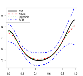
(a) $N=50$

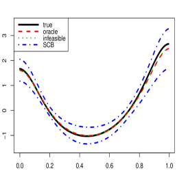
(b) $N=200$

Figure 1: Plot of true covariance function (thick solid line), oracle estimator $\widehat{C}$ (dashed line) and the $99\%$ SCB (dotted-dashed line), infeasible estimator $\widetilde{C}$ (dotted line) for the covariance function with $\sigma_{\epsilon}=0.1$.

5.2 Spatial covariance models

In order to compare the finite-sample performance of the proposed estimator to that of Cao et al. (2016), we consider the following spatial covariance models:

• Spherical model (M1): $C(h;\sigma_{s}^{2},\theta_{s})=\sigma_{s}^{2}\{1-\frac{3}{2}\frac{h}{\theta_{s}}+\frac{1}{2}(\frac{h}{\theta_{s}})^{3}\}I\left\{h\leq\theta_{s}\right\}$;

• Matérn model (M2): $C(h;\sigma_{s}^{2},\theta_{s},v)=\sigma_{s}^{2}\left\{\Gamma(v)\right\}^{-1}2^{1-v}\left(2\sqrt{v}h/\theta_{s}\right)^{v}\digamma_{v}\left(2\sqrt{v}h/\theta_{s}\right),$ where $\Gamma$ is the gamma function, $\digamma_{v}$ is the modified Neumann function;

• Gaussian Model (M3): $C(h;\sigma_{s}^{2},\theta_{s})=\sigma_{s}^{2}\exp(-h^{2}/\theta_{s}^{2})$.

In the parameterization (following Banerjee et al. (2004) page 29) of the covariance structure, $\sigma_{s}^{2}$ is the sill and $\theta_{s}$ is the range parameter. In the simulation, we set $\sigma_{s}^{2}$ $=2$ for M1, M2 and M3, and choose $\theta_{s}=1$ for M1 and M2, $\theta_{s}=3$ for M3, while for M2, $v=3$. Since $C\left(h\right)\rightarrow 0$ as $h\rightarrow\infty$, in practice, we only numerically evaluate the covariance $C\left(h\right)$ over the “effective range” defined as the distance beyond which the correlation between observations, $\rho(h)=C\left(h\right)/C\left(0\right)$, is less than or equal to $0.05$. In such sense, we choose the compact interval $[0,s]$ to represent the “effective range”, where $s$ is the largest $h$ satisfying $\rho(h)\leq 0.05$. An exception of this phenomenon is the spherical model that has an exact range $\left[0,\theta_{s}\right]$, i.e., $C\left(h\right)=0$ when $h=\theta_{s}$. To be consistent in our evaluation of the methods, we apply the “effective range” to the spherical model as well.

Our data are generated from $Y_{ij}=m(x_{j})+Z_{i}\left(x_{j}\right)+\sigma\left(x_{j}\right)\varepsilon_{ij}$, where $m(x)=\sin\{2\pi\left(x-1/2\right)\}$, $\{x_{j}\}_{j=1}^{N}$ are equally spaced grid points over “effective range” $[0,s]$, $\varepsilon_{ij}$ $\sim N(0,1)$ are i.i.d variables, and the process $Z_{i}(\cdot)$ is generated from a zero mean Gaussian process. We examine the performance of models containing homogeneous errors with $\sigma(x)=\sigma_{\epsilon}$ and heteroscedastic errors with $\sigma(x)=\sigma_{\epsilon}\frac{5-\exp\left(x/2\right)}{5+\exp\left(x/2\right)}$ for M1, and $\sigma(x)=\sigma_{\epsilon}\frac{30-\exp\left(x/2\right)}{30+\exp\left(x/2\right)}$ for M2 and M3. The results are similar to each other, so we only present the results with homogeneous errors. The number of curves $n=\lfloor 0.8N\rfloor$ with $N=50$, $100$ and $200$, and the noise levels are $\sigma_{\epsilon}=0.1,~{}0.5$. The mean function is estimated by cubic splines, i.e., $p=4$, with the number of knots selected using the formula given in Section 4.2. The GCV selected knots yield similar results but it is more time consuming, hence they are not summarized here.

The AMSE of the covariance estimators $\widehat{C}$ and $\widetilde{C}$ are reported in columns 4–5 of Table 3. The performance of the two estimators is very similar. Columns 6 and 8 present the empirical coverage rate CR, i.e., the percentage of the true curve $C(\cdot)$ entirely covered by the SCB, based on $95\%$ and $99\%$ confidence levels, respectively. As the sample size increases, the coverage probability of the SCB becomes closer to the nominal confidence level. In addition, the WDs of the bands are calculated and presented in columns 7 and 9 in Table 3. It is obvious that the width tends to be narrower when the sample size becomes larger or $\sigma_{\epsilon}$ is smaller.

Table 3: Simulation results based on homogeneous errors with $\sigma(x)=\sigma_{\epsilon}$: AMSE of estimators $\widehat{C}$, $\widetilde{C}$; CR (outside/inside of the parentheses is based on $\widehat{C}$ and $\widetilde{C}$), and WD of SCBs based on $\widehat{C}$.

$\sigma_{\epsilon}$	Model	$N$	AMSE			SCB
			$\widehat{C}$	$\widetilde{C}$		$95\%$			$99\%$
						CR	WD		CR	WD
$0.1$	M1	$50$	$0.082$	$0.081$		$0.910(0.918)$	$1.37$		$0.960(0.966)$	$1.68$
		$100$	$0.040$	$0.040$		$0.920(0.926)$	$0.99$		$0.974(0.978)$	$1.21$
		$200$	$0.019$	$0.018$		$0.946(0.952)$	$0.72$		$0.980(0.986)$	$0.87$
	M2	$50$	$0.096$	$0.095$		$0.904(0.908)$	$1.44$		$0.950(0.954)$	$1.78$
		$100$	$0.048$	$0.049$		$0.926(0.924)$	$1.05$		$0.978(0.978)$	$1.30$
		$200$	$0.022$	$0.022$		$0.958(0.958)$	$0.76$		$0.992(0.994)$	$0.94$
	M3	$50$	$0.109$	$0.109$		$0.906(0.910)$	$1.50$		$0.954(0.958)$	$1.86$
		$100$	$0.055$	$0.055$		$0.922(0.928)$	$1.09$		$0.976(0.978)$	$1.35$
		$200$	$0.025$	$0.025$		$0.960(0.958)$	$0.79$		$0.988(0.990)$	$0.98$
$0.5$	M1	$50$	$0.082$	$0.080$		$0.896(0.912)$	$1.38$		$0.952(0.964)$	$1.70$
		$100$	$0.040$	$0.040$		$0.920(0.928)$	$0.99$		$0.980(0.980)$	$1.21$
		$200$	$0.019$	$0.018$		$0.938(0.946)$	$0.72$		$0.988(0.988)$	$0.88$
	M2	$50$	$0.097$	$0.096$		$0.896(0.908)$	$1.46$		$0.946(0.958)$	$1.80$
		$100$	$0.048$	$0.049$		$0.914(0.930)$	$1.06$		$0.978(0.980)$	$1.30$
		$200$	$0.022$	$0.022$		$0.954(0.958)$	$0.77$		$0.990(0.994)$	$0.94$
	M3	$50$	$0.111$	$0.111$		$0.908(0.916)$	$1.51$		$0.952(0.962)$	$1.88$
		$100$	$0.055$	$0.055$		$0.912(0.924)$	$1.10$		$0.974(0.978)$	$1.36$
		$200$	$0.025$	$0.025$		$0.958(0.956)$	$0.79$		$0.988(0.990)$	$0.98$

When the covariance structure is not necessarily stationary, Cao et al. (2016) proposed a tensor-product bivariate B-spline estimator $\widehat{G}^{\mathrm{TPS}}(x,x^{\prime})$ and a SCB for the covariance function $G(x,x^{\prime})=\mathrm{Cov}\left\{Z_{1}(x),Z_{1}\left(x^{\prime}\right)\right\}$.  Following the suggestion of one referee, to assess the accuracy of recovering $G(\cdot,\cdot)$, the covariance function estimators $\widehat{C}$ is also presented in 2D to make a comparison, say, $\widehat{G}^{\mathrm{PROP}}(x,x^{\prime})=\widehat{C}(\left|x-x^{\prime}\right|)$. In addition, the simultaneous confidence envelops (SCE) is constructed by using $\widehat{G}^{\mathrm{PROP}}(x,x^{\prime})$ and $\widehat{G}^{\mathrm{TPS}}(x,x^{\prime})$ are compared, named SCE-I and SCE-II, respectively.

Columns 4–5 of Table 4 present the AMSEs of $\widehat{G}^{\mathrm{PROP}}(x,x^{\prime})$ and $\widehat{G}^{\mathrm{TPS}}(x,x^{\prime})$. The results of AMSEs indicate that $\widehat{G}^{\mathrm{PROP}}$ is more accurate than $\widehat{G}^{\mathrm{TPS}}$, while $\widehat{G}^{\mathrm{TPS}}$ usually gives larger AMSE. Columns 6–13 of Table 4 report the CR and WD of SCE-I and SCE-II. One sees that the CRs of SCE-I are much closer to the nominal levels than those of SCE-II, and increasing the sample size helps to improve the CR of the SCEs to their nominal levels. One also observes the widths of the SCE-I are much narrower than those of the SCE-II. These findings indicate our proposed SCE-I is more efficient than SCE-II when the true covariance function is stationary.

Table 4: Simulation results based on homogeneous errors with $\sigma(x)=\sigma_{\epsilon}$: AMSE of estimators $\widehat{G}^{\mathrm{PROP}}(\cdot,\cdot)$, $\widehat{G}^{\mathrm{TPS}}(\cdot,\cdot)$; CR and WD of SCE-I and SCE-II.

$\sigma_{\epsilon}$	Model	$N$	AMSE			SCE-I					SCE-II
			$\widehat{G}^{\mathrm{PROP}}$	$\widehat{G}^{\mathrm{TPS}}$		$95\%$		$99\%$			$95\%$		$99\%$
						CR	WD	CR	WD		CR	WD	CR	WD
$0.1$	M1	$50$	$0.079$	$0.123$		$0.910$	$1.40$	$0.960$	$1.71$		$0.744$	$2.08$	$0.840$	$2.55$
		$100$	$0.039$	$0.063$		$0.920$	$1.01$	$0.974$	$1.24$		$0.852$	$1.64$	$0.944$	$2.02$
		$200$	$0.018$	$0.031$		$0.946$	$0.73$	$0.980$	$0.90$		$0.904$	$1.19$	$0.964$	$1.47$
	M2	$50$	$0.096$	$0.148$		$0.904$	$1.50$	$0.950$	$1.86$		$0.682$	$2.09$	$0.816$	$2.56$
		$100$	$0.048$	$0.072$		$0.926$	$1.10$	$0.978$	$1.35$		$0.780$	$1.62$	$0.898$	$2.00$
		$200$	$0.022$	$0.036$		$0.958$	$0.79$	$0.992$	$0.98$		$0.926$	$1.16$	$0.976$	$1.43$
	M3	$50$	$0.114$	$0.153$		$0.906$	$1.57$	$0.954$	$1.95$		$0.724$	$2.15$	$0.824$	$2.65$
		$100$	$0.057$	$0.074$		$0.922$	$1.15$	$0.976$	$1.42$		$0.852$	$1.52$	$0.942$	$1.86$
		$200$	$0.026$	$0.039$		$0.960$	$0.83$	$0.988$	$1.21$		$0.882$	$1.09$	$0.956$	$1.33$
$0.5$	M1	$50$	$0.079$	$0.133$		$0.896$	$1.41$	$0.952$	$1.73$		$0.740$	$2.10$	$0.858$	$2.58$
		$100$	$0.039$	$0.064$		$0.920$	$1.02$	$0.980$	$1.25$		$0.814$	$1.64$	$0.924$	$2.03$
		$200$	$0.018$	$0.032$		$0.938$	$0.74$	$0.988$	$0.90$		$0.896$	$1.19$	$0.968$	$1.46$
	M2	$50$	$0.097$	$0.146$		$0.898$	$1.51$	$0.946$	$1.87$		$0.666$	$2.13$	$0.780$	$2.60$
		$100$	$0.048$	$0.071$		$0.914$	$1.10$	$0.978$	$1.35$		$0.768$	$1.62$	$0.906$	$2.00$
		$200$	$0.022$	$0.036$		$0.954$	$0.79$	$0.990$	$0.98$		$0.928$	$1.16$	$0.970$	$1.43$
	M3	$50$	$0.115$	$0.161$		$0.908$	$1.58$	$0.952$	$1.97$		$0.694$	$2.16$	$0.792$	$2.65$
		$100$	$0.057$	$0.075$		$0.912$	$1.15$	$0.974$	$1.42$		$0.814$	$1.53$	$0.928$	$1.87$
		$200$	$0.026$	$0.037$		$0.958$	$0.83$	$0.988$	$1.03$		$0.864$	$1.09$	$0.956$	$1.33$

6 Real data analysis

To further illustrate our methodology, we first consider the modeling of the Gait Data collected by the Motion Analysis Laboratory at the Children’s Hospital in San Diego, CA. We focus on the “Hip Angle” functional dataset, which consists of the angles formed by the hip of each boy over his gait cycle. See Olshen et al. (1989) for the details. In the study, the cycle begins and ends at the point where the heel of the limb under observation strikes the ground, which has been translated into values over $[0,1]$. There are measurements on $n=39$ samples (boys), where for each sample $N=20$ hip angles were recorded every $0.05$ second with time being measured on $[0,1]$. Denote by $Y_{ij}$ the hip angle of the $i$th boy at the time $x_{j}$, $j=1,\ldots,N$ and $i=1,\ldots,n$. Figure 2 (a) shows hip curves together with their estimated mean curve, and Figure 2 (b) describes the 3D shape of all curves, where “time” is plotted on one axis and sample index on the other.

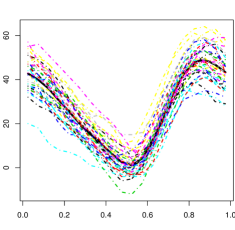
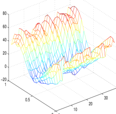
Figure 2: (a) Hip angle data (dotted lines) with its mean function estimator (solid line); (b) 3D plot.

Figure 3 (a) and (b) display the 3D and contour plots of the sample correlation of the hip data. From the plot, the contours are almost parallel to the main diagonal, indicating that the variation of the hip angles can be considered as an approximately stationary process. Figure 4 (a) shows a 3D plot of the proposed covariance matrix estimator $\widehat{G}^{\mathrm{PROP}}(x,x^{\prime})=\widehat{C}(|x-x^{\prime}|)$ with its asymptotic SCE. For comparison, the nonstationary covariance function estimator $\widehat{G}^{\mathrm{TPS}}$ and its SCE are also presented; see Figure 4 (b).

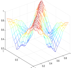
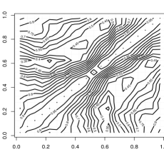
Figure 3: (a): Unsmoothed sample correlation 3D plot for the hip angle data; (b): Unsmoothed sample correlation contour plot for the hip angle data.

As mentioned in Section 1, SCB is a very insightful and useful tool to examine the adequacy of certain parametric specifications of a covariance function. Now we make use of the proposed SCB to test if this hip data has a parametric covariance form like M1, M2 or M3. We set the null hypothesis $H_{0}$ for M1, M2 and M3 in the following:

$$\text{M1 }H_{0} \text{:}\text{ }C\left(h\right)=C\left(h;32,\theta_{s}\right)=32\{1-1.5\left(h/\theta_{s}\right)+0.5(h/\theta_{s})^{3}\}I\left\{h\leq\theta_{s}\right\}\text{,}$$ (12)

$$\text{M2 }H_{0} \text{:}\text{ }C\left(h\right)=C(h;32,\theta_{s},\nu)=32\left\{\Gamma\left(v\right)\right\}^{-1}2^{1-v}\left\{2\sqrt{v}h/\theta_{s}\right\}^{v}\digamma_{v}\left(2\sqrt{v}h/\theta_{s}\right)\text{,}$$ (13)

$$\text{M3 }H_{0} \text{:}\text{ }C\left(h\right)=C(h;32,\theta_{s})=32\exp(-h^{2}/\theta_{s}^{2}),$$ (14)

where $\theta_{s}=1.12$ for M1 and M2, $v=1.2$ for M2 and $\theta_{s}=2.19$ for M3. In Figure 5, the thick solid line is the covariance function $C\left(h\right)$ under $H_{0}$, the center dashed line is the B-spline estimator , and the dotted-dashed lines are the SCBs. From Figure 5 (a), one observes that even the $99\%$ SCB cannot contain $C\left(h;32,1.12\right)$, hence the null hypothesis in (12) is rejected with $p$-value $<0.01$. Figure 5 (b) and (c) indicate that the $80\%$ SCB contains $C\left(h;32,1.2,1.12\right)$ and $C\left(h;32,2.19\right)$, the null hypothesis in (13) and (14) is not rejected with $p$-value $>0.2$.

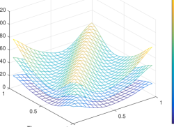
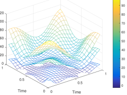
Figure 4: (a): Covariance matrix estimator based on $\widehat{G}^{\mathrm{PROP}}(x,x^{\prime})$ (middle) with $95\%$ SCE (up and below); (b): covariance matrix estimator $\widehat{G}^{\mathrm{TPS}}(x,x^{\prime})$ (middle) of Cao et al. (2016) with $95\%$ SCE (up and below).

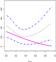
(a) 99% SCB for M1

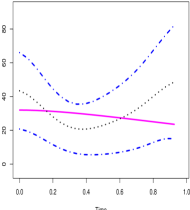
(b) 80% SCB for M2

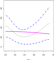
(c) 80% SCB for M3

Figure 5: Covariance function $C\left(h\right)$ under $H_{0}$ (thick solid line), B-spline covariance estimator $\widehat{C}$ (dotted line), and the SCB based on $\widehat{C}$ (dotted-dashed line) for the hip angle data.

A. Technical Lemmas and Proofs of Propositions 1 and 2

Throughout this section, $\mathcal{O}_{p}$ (or ${\scriptstyle{\mathcal{O}}}_{p}$) denotes a sequence of random variables of certain order in probability. For instance, ${\scriptstyle{\mathcal{O}}}_{p}(n^{-1/2})$ means a smaller order than $n^{-1/2}$ in probability, and by $\mathcal{O}_{a.s.}$ (or ${\scriptstyle{\mathcal{O}}}_{a.s.}$) almost surely $\mathcal{O}$ (or ${\scriptstyle{\mathcal{O}}}$). In addition, $\mathcal{U}_{p}$ denotes a sequence of random functions which are $\mathcal{O}_{p}$ uniformly defined in the domain.

For any vector $\mathbf{a}=\left(a_{1},\ldots,a_{n}\right)\in\mathcal{R}^{n}$, denote the norm $\left\|\mathbf{a}\right\|_{r}=(\left|a_{1}\right|^{r}+$ $\cdots$ $+\left|a_{n}\right|^{r})^{1/r}$, $1\leq r<+\infty$, $\left\|\mathbf{a}\right\|_{\infty}=\max\left(\left|a_{1}\right|,\ldots,\left|a_{n}\right|\right)$. For any matrix $\mathbf{A}=\left(a_{ij}\right)_{i=1,j=1}^{m,n}$, denote its $L_{r}$ norm as $\left\|\mathbf{A}\right\|_{r}=\max_{\mathbf{a}\in\mathcal{R}^{n},\mathbf{a}\neq\mathbf{0}}\left\|\mathbf{Aa}\right\|_{r}$ $\left\|\mathbf{a}\right\|_{r}^{-1}$, for $r<+\infty$ and $\left\|\mathbf{A}\right\|_{r}=\max_{1\leq i\leq m}\sum_{j=1}^{n}\left|a_{ij}\right|$, for $r=\infty$.

A.1 Lemmas

Let $\mathbf{Y}_{i}=\left(Y_{i1},\ldots,Y_{iN}\right)^{\top}$, then the spline estimator $\widehat{\eta}_{i}(x)$ in (5) can be represented as $\widehat{\eta}_{i}(x)=\mathbf{B}(x)^{\top}(\mathbf{B}^{\top}\mathbf{B})^{-1}\mathbf{B}^{\top}\mathbf{Y}_{i}$, where $\mathbf{B}$ is given in (10). Define the empirical inner product matrix of B-spline basis $\left\{B_{\ell,p}(x)\right\}_{\ell=1}^{J_{s}+p}$ as $\mathbf{V}_{n,p}=\left\{\left\langle B_{\ell,p},B_{\ell^{\prime},p}\right\rangle_{N}\right\}_{\ell,\ell^{\prime}=1}^{J_{s}+p}=N^{-1}\mathbf{B}^{\top}\mathbf{B}$, and according to Lemma A.3 in Cao et al. (2012), for some constant $C_{p}>0$

$$\left\|\mathbf{V}_{n,p}^{-1}\right\|_{\infty}\leq C_{p}J_{s}.$$ (A.1)

According to model (2), $\mathbf{\eta}_{i}=\mathbf{m}+\mathbf{Z}_{i}$, where $\mathbf{\eta}_{i}=\left\{\eta_{i}\left(1/N\right),\ldots,\eta_{i}\left(N/N\right)\right\}^{\top}$, $\mathbf{Z}_{i}=\left\{Z_{i}\left(1/N\right),\ldots,Z_{i}\left(N/N\right)\right\}^{\top}$, $\mathbf{m}=\left\{m\left(1/N\right),\ldots,m\left(N/N\right)\right\}^{\top}$, then the approximation error $\widehat{\eta}_{i}(x)-\eta_{i}(x)$ can be decomposed into the following:

$$\widehat{\eta}_{i}(x)-\eta_{i}(x)=\widetilde{\eta}_{i}(x)-\eta_{i}(x)+\widetilde{\varepsilon}_{i}(x),$$ (A.2)

where $\widetilde{\varepsilon}_{i}(x)=N^{-1}\mathbf{B}(x)^{\mathbf{\top}}\mathbf{V}_{n,p}^{-1}\mathbf{B}^{\top}\mathbf{\varepsilon}_{i}$, and

$$\widetilde{\eta}_{i}(x) =N^{-1}\mathbf{B}(x)^{\top}\mathbf{V}_{n,p}^{-1}\mathbf{B}^{\top}\mathbf{\eta}_{i}=\widetilde{m}(x)+\widetilde{Z}_{i}(x),$$ (A.3)

$$\widetilde{m}(x) =N^{-1}\mathbf{B}(x)^{\top}\mathbf{V}_{n,p}^{-1}\mathbf{B}^{\top}\mathbf{m},~{}\widetilde{Z}_{i}(x)=N^{-1}\mathbf{B}(x)^{\mathbf{\top}}\mathbf{V}_{n,p}^{-1}\mathbf{B}^{\top}\mathbf{Z}_{i},$$ (A.4)

where $\mathbf{\varepsilon}_{i}=(\sigma\left(1/N\right)\varepsilon_{i1},\ldots,\sigma\left(N/N\right)\varepsilon_{iN})^{\top}$. Thus, one has $\widehat{\eta}_{i}(x)-\eta_{i}(x)=\widetilde{Z}_{i}(x)-Z_{i}(x)+\widetilde{m}(x)-m(x)+\widetilde{\varepsilon}_{i}(x)$. Therefore, by (4), (6) and (A.2), the approximation error of $\widehat{Z}_{i}(x)$ in (4) to $Z_{i}(x)$ can be represented by

$$\widehat{Z}_{i}(x)-Z_{i}(x)=\widetilde{Z}_{i}(x)-Z_{i}(x)+\widetilde{\varepsilon}_{i}(x)-\frac{1}{n}\sum_{i^{\prime}=1}^{n}\left\{\widetilde{Z}_{i^{\prime}}(x)+\widetilde{\varepsilon}_{i^{\prime}}(x)\right\}.$$ (A.5)

Lemma A.1.

Under Assumptions (A1)–(A6), as $N\rightarrow\infty$, one has

$$\max_{1\leq i\leq n}\left\|\widetilde{\eta}_{i}-\eta_{i}\right\|_{\infty} =\mathcal{O}_{a.s.}\{J_{s}^{-p^{*}}\left(n\log n\right)^{2/r_{1}}\},$$ (A.6)

$$\max_{1\leq i\leq n}\|\widetilde{Z}_{i}-Z_{i}\|_{\infty}=\mathcal{O}_{a.s.}\{J_{s}^{-p^{*}}(n\log n)^{2/r_{1}}\}, ~{}\max_{1\leq i\leq n}\left\|Z_{i}\right\|_{\infty}=\mathcal{O}_{a.s.}\{(n\log n)^{2/r_{1}}\}.$$

Lemma A.2.

Under Assumptions (A1)–(A6), as $N\rightarrow\infty$, one has

$$\max_{1\leq i\leq n}\left\|\widetilde{\varepsilon}_{i}\right\|_{\infty}=\mathcal{O}_{a.s}\{J_{s}^{1/2}N^{-1/2}(\log N)^{1/2}\}.$$

The next lemma follows from Lemmas A.1, A.2, (A.2) and (A.5).

Lemma A.3.

Under Assumptions (A1)–(A6), as $N\rightarrow\infty$,

$$\max_{1\leq i\leq n}\left\|\widehat{\eta}_{i}-\eta_{i}\right\|_{\infty} =\mathcal{O}_{p}\left\{J_{s}^{-p^{*}}\left(n\log n\right)^{2/r_{1}}+J_{s}^{1/2}N^{-1/2}\left(\log N\right)^{1/2}\right\},$$

$$\max_{1\leq i\leq n}\|\widehat{Z}_{i}-Z_{i}\|_{\infty} =\mathcal{O}_{p}\left\{J_{s}^{-p^{*}}\left(n\log n\right)^{2/r_{1}}+J_{s}^{1/2}N^{-1/2}\left(\log N\right)^{1/2}\right\}.$$ (A.7)

Lemma A.4.

Assumption (A5) holds under Assumptions (A4) and (A5’).

Lemma A.5.

Under Assumptions (A1)–(A6),

$$\sup_{h\in\left[0,h_{0}\right]}\left|\frac{1}{n(1-h)}\int_{0}^{1-h}\sum_{i=1}^{n}Z_{i}(x+h)\left\{\widetilde{Z}_{i}(x)-Z_{i}(x)\right\}dx\right|={\scriptstyle{\mathcal{O}}}_{p}(n^{-1/2}).$$

Lemma A.6.

Under Assumptions (A1)–(A6),

$$\max_{1\leq i\leq n}\max_{1\leq\ell\leq J_{s}+p}\left|N^{-1}\sum_{j=1}^{N}B_{\ell,p}(j/N)\sigma\left(j/N\right)U_{ij,\varepsilon}\right|=\mathcal{O}_{a.s.}(N^{-1/2}J_{s}^{-1/2}\log^{1/2}N),$$

where $U_{ij,\varepsilon}$, $1\leq i\leq n$, $1\leq j\leq N$, are iid standard normal random variables.

Lemma A.7.

Under Assumptions (A1)–(A6),

$$\max_{1\leq k\leq k_{n}\atop 1\leq\ell\leq J_{s}+p}\left|\frac{1}{nN}\sum_{i=1}^{n}U_{ik,\xi}\left\{\sum_{j=1}^{N}B_{\ell,p}\left(\frac{j}{N}\right)\sigma\left(j/N\right)(\varepsilon_{ij}-U_{ij,\varepsilon})\right\}\right|=\mathcal{O}_{a.s.}\left(n^{-1/2}N^{\beta_{2}-1}\log^{1/2}N\right),$$

where $0<\beta_{2}<1/2$.

Lemma A.8.

Under Assumptions (A1)–(A6), one has

$$\max_{1\leq k\leq k_{n}\atop 1\leq\ell\leq J_{s}+p}\left|(nN)^{-1}\sum_{i=1}^{n}\left(\xi_{ik}-U_{ik,\xi}\right)\sum_{j=1}^{N}B_{\ell,p}\left(\frac{j}{N}\right)\sigma\left(\frac{j}{N}\right)U_{ij,\varepsilon}\right|$$

$$=\mathcal{O}_{a.s.}(n^{\beta_{1}-1/2}N^{-1/2}J_{s}^{-1/2}\log^{1/2}N),\textrm{~{} for ~{}}0<\beta_{1}<1/2.$$

Lemma A.9.

Under Assumptions (A2)–(A6),

$$\max_{1\leq k\leq k_{n}\atop 1\leq\ell\leq J_{s}+p}\left|\frac{1}{nN}\sum_{i=1}^{n}\left(\xi_{ik}-U_{ik,\xi}\right)\left\{\sum_{j=1}^{N}B_{\ell,p}\left(\frac{j}{N}\right)\sigma\left(\frac{j}{N}\right)(\varepsilon_{ij}-U_{ij,\varepsilon})\right\}\right|=\mathcal{O}_{a.s.}\left(n^{\beta_{1}}N^{\beta_{2}-1}\right).$$

Lemma A.10.

Under Assumptions (A2)–(A6),

$$\sup_{h\in\left[0,h_{0}\right]}\sup_{x\in\left[0,1\right]}\left|\frac{1}{n}\sum_{i=1}^{n}Z_{i}(x+h)\widetilde{\varepsilon}_{i}(x)\right|={\scriptstyle{\mathcal{O}}}_{p}(n^{-1/2}).$$

Lemma A.11.

Under Assumptions (A2)–(A6), one has

$$\sup_{h\in\left[0,h_{0}\right]}\sup_{x\in\left[0,1\right]}\left|\frac{1}{n}\sum\limits_{i=1}^{n}Z_{i}(x+h)\frac{1}{n}\sum\limits_{i^{\prime}=1}^{n}\widetilde{Z}_{i^{\prime}}(x)\right|={\scriptstyle{\mathcal{O}}}_{p}(n^{-1/2}).$$

Lemma A.12.

Let $W_{i}\sim N\left(0,\sigma_{i}^{2}\right),\sigma_{i}>0,i=1,\ldots,n$, then for $a>2$

$$\Pr\left(\max_{1\leq i\leq n}\left|W_{i}/\sigma_{i}\right|>a\sqrt{\log n}\right)<2n^{1-a^{2}/2}.$$ (A.8)

Hence, $\left(\max_{1\leq i\leq n}\left|W_{i}\right|\right)/\left(\max_{1\leq i\leq n}\sigma_{i}\right)\leq\max_{1\leq i\leq n}\left|W_{i}/\sigma_{i}\right|={{\mathcal{O}}}_{a.s.}\left(\sqrt{\log n}\right)$.

A.2 Proof of Proposition 1

Let $\mathcal{F}_{t}=\sigma\left(\bar{\xi}_{\cdot 11},\bar{\xi}_{\cdot 12},\ldots,\bar{\xi}_{\cdot 1t},\bar{\xi}_{\cdot 22},\ldots,\bar{\xi}_{\cdot t-1,t},\bar{\xi}_{\cdot tt}\right)$, so that $\mathcal{F}_{2}\subseteq\mathcal{F}_{3}\subseteq\mathcal{F}_{4}\subseteq\mathcal{\cdots}$ is an increasing sequence of $\sigma$-fields. Denote

$$S_{t}(h)= \sqrt{n}\Delta(\cdot)=\sqrt{n}\textstyle\sum\limits_{1\leq k\neq k^{\prime}\leq t}\bar{\xi}_{\cdot kk^{\prime}}\frac{1}{1-h}\int_{0}^{1-h}\phi_{k}(x)\phi_{k^{\prime}}(x+h)dx$$

$$+\sqrt{n}\textstyle\sum\limits_{1\leq k\leq t}\left(\bar{\xi}_{\cdot kk}-1\right)\frac{1}{1-h}\int_{0}^{1-h}\phi_{k}(x)\phi_{k}(x+h)dx,$$

for $t=1,\ldots,k_{n}$, where $k_{n}$ satisfies Assumption (A4). We show that $S_{t}(h)$ is a martingale process in $h\in\left[0,h_{0}\right]$.

Define $D_{t}(h)=S_{t}(h)-S_{t-1}(h)$, thus,

$$D_{t}(h)=\frac{\sqrt{n}}{1-h}\left\{\textstyle\sum\limits_{k=1}^{t-1}\bar{\xi}_{\cdot kt}\int_{0}^{1-h}\left\{\phi_{k}(x)\phi_{t}(x+h)+\phi_{t}(x)\phi_{k}(x+h)\right\}dx+\left(\bar{\xi}_{\cdot tt}-1\right)\int_{0}^{1-h}\phi_{t}(x)\phi_{t}(x+h)dx\right\},$$

which is $\mathcal{F}_{t}$-measurable. While notice that for any $t$,

$$\mathrm{E}\left(\left.D_{t}(h)\right|\mathcal{F}_{t-1}\right)=\frac{\sqrt{n}}{1-h}\mathrm{E}\left\{\textstyle\sum\limits_{k=1}^{t-1}\bar{\xi}_{\cdot kt}\int_{0}^{1-h}\left\{\phi_{k}(x)\phi_{t}(x+h)+\phi_{t}(x)\phi_{k}(x+h)\right\}dx\right.$$

$$\quad\left.\left.+\left(\bar{\xi}_{\cdot tt}-1\right)\int_{0}^{1-h}\phi_{t}(x)\phi_{t}(x+h)dx\right|\mathcal{F}_{t-1}\right\}$$

$$=\frac{\sqrt{n}}{1-h}\mathrm{E}\left\{\left.\frac{1}{n}\textstyle\sum\limits_{i=1}^{n}\xi_{it}\textstyle\sum\limits_{k=1}^{t-1}\xi_{ik}\int_{0}^{1-h}\left\{\phi_{k}(x)\phi_{t}(x+h)+\phi_{t}(x)\phi_{k}(x+h)\right\}dx\right|\mathcal{F}_{t-1}\right\}$$

$$\quad+\sqrt{n}\mathrm{E}\left\{\left.\left(\bar{\xi}_{\cdot tt}-1\right)\int_{0}^{1-h}\phi_{t}(x)\phi_{t}(x+h)dx\right|\mathcal{F}_{t-1}\right\}=0,$$

which implies that $\left\{D_{t}(h),t=2,3,\ldots\right\}$ is a martingale difference process with respect to $\left\{\mathcal{F}_{t-1},t=2,3,\ldots\right\}$.

Next denote

$$\mathrm{E}\left(\left.D_{t}^{2}(h)\right|\mathcal{F}_{t-1}\right)=\mathrm{V}_{t}^{\left(1\right)}(h)+\mathrm{V}_{t}^{\left(2\right)}(h)+\mathrm{V}_{t}^{\left(3\right)}(h),$$ (A.9)

in which

$$\mathrm{V}_{t}^{\left(1\right)}(h)= n\mathrm{E}\left[\left.\left\{n^{-1}\textstyle\sum\limits_{i=1}^{n}\xi_{it}\textstyle\sum\limits_{k=1}^{t-1}\xi_{ik}\frac{1}{1-h}\int_{0}^{1-h}\left\{\phi_{k}(x)\phi_{t}(x+h)+\phi_{t}(x)\phi_{k}(x+h)\right\}dx\right\}^{2}\right|\mathcal{F}_{t-1}\right],$$

$$\mathrm{V}_{t}^{\left(2\right)}(h)= n\mathrm{E}\left[\left.\left\{\left(\bar{\xi}_{\cdot tt}-1\right)\frac{1}{1-h}\int_{0}^{1-h}\phi_{t}(x)\phi_{t}(x+h)dx\right\}^{2}\right|\mathcal{F}_{t-1}\right],$$

$$\mathrm{V}_{t}^{\left(3\right)}(h)= 2n\mathrm{E}\left[\left\{n^{-1}\textstyle\sum\limits_{i=1}^{n}\xi_{it}\textstyle\sum\limits_{k=1}^{t-1}\xi_{ik}\frac{1}{1-h}\int_{0}^{1-h}\left\{\phi_{k}(x)\phi_{t}(x+h)+\phi_{t}(x)\phi_{k}(x+h)\right\}dx\right\}\right.$$

$$\times\left.\left.\left(\bar{\xi}_{\cdot tt}-1\right)\frac{1}{1-h}\int_{0}^{1-h}\phi_{t}(x)\phi_{t}(x+h)dx\right|\mathcal{F}_{t-1}\right].$$

Moreover, one can show that

$$\mathrm{V}_{t}^{\left(1\right)}(h) =\mathrm{E}\left[\left.\left\{\frac{1}{n}\textstyle\sum\limits_{i=1}^{n}\xi_{it}\textstyle\sum\limits_{k=1}^{t-1}\xi_{ik}\frac{1}{1-h}\int_{0}^{1-h}\left\{\phi_{k}(x)\phi_{t}(x+h)+\phi_{t}(x)\phi_{k}(x+h)\right\}dx\right\}^{2}\right|\mathcal{F}_{t-1}\right]$$

$$=\mathrm{E}\textstyle\sum\limits_{k=1}^{t-1}\left[\left.\frac{1}{n}\textstyle\sum\limits_{i=1}^{n}\xi_{it}^{2}\xi_{ik}^{2}\left(\frac{1}{1-h}\int_{0}^{1-h}\left\{\phi_{k}(x)\phi_{t}(x+h)+\phi_{t}(x)\phi_{k}(x+h)\right\}dx\right)^{2}\right|\mathcal{F}_{t-1}\right]$$

$$=\mathrm{E}\xi_{1t}^{2}\textstyle\sum\limits_{k=1}^{t-1}\bar{\xi}_{\cdot kk}\left[\frac{1}{1-h}\int_{0}^{1-h}\left\{\phi_{k}(x)\phi_{t}(x+h)+\phi_{t}(x)\phi_{k}(x+h)\right\}dx\right]^{2},$$

therefore, one has when $n\rightarrow\infty$,

$$\textstyle\sum\limits_{t=2}^{k_{n}} \mathrm{V}_{t}^{\left(1\right)}(h)\rightarrow\textstyle\sum\limits_{k\neq k^{\prime}}^{\infty}\left\{\frac{1}{1-h}\int_{0}^{1-h}\phi_{k}(x)\phi_{k^{\prime}}(x+h)dx\right\}^{2}$$

$$+\textstyle\sum\limits_{k\neq k^{\prime}}^{\infty}\left\{\frac{1}{1-h}\int_{0}^{1-h}\phi_{k}(x)\phi_{k^{\prime}}(x+h)dx\right\}\left\{\frac{1}{1-h}\int_{0}^{1-h}\phi_{k}(x+h)\phi_{k^{\prime}}(x)dx\right\}<\infty.$$

Note that $\mathrm{V}_{t}^{\left(2\right)}(h)=\left(\mathrm{E}\xi_{1t}^{4}-1\right)\left\{(1-h)^{-1}\int_{0}^{1-h}\phi_{t}(x)\phi_{t}(x+h)dx\right\}^{2}<\infty$, so one has that $\textstyle\sum_{t=2}^{k_{n}}\mathrm{V}_{t}^{\left(2\right)}\left(h\right)\rightarrow\textstyle\sum_{k=1}^{\infty}\left(\mathrm{E}\xi_{1k}^{4}-1\right)\left\{(1-h)^{-1}\int_{0}^{1-h}\phi_{k}(x)\phi_{k}(x+h)dx\right\}^{2}<\infty$. Similarly,

$$\mathrm{V}_{t}^{\left(3\right)}(h) =2n\mathrm{E}\left[\left\{\textstyle\sum\limits_{k=1}^{t-1}\frac{1}{n}\textstyle\sum\limits_{i=1}^{n}\xi_{it}\xi_{ik}\frac{1}{1-h}\int_{0}^{1-h}\left\{\phi_{k}(x)\phi_{t}(x+h)+\phi_{t}(x)\phi_{k}(x+h)\right\}dx\right\}\right.$$

$$\times\left.\left(\frac{1}{n}\textstyle\sum\limits_{i=1}^{n}\xi_{it}^{2}-1\right)\frac{1}{1-h}\int_{0}^{1-h}\phi_{t}(x)\phi_{t}(x+h)dx\mathcal{F}_{t-1}\right]$$

$$=2\left(\mathrm{E}\xi_{1t}^{3}-1\right)\mathrm{E}\left[\textstyle\sum\limits_{k=1}^{t-1}\bar{\xi}_{\cdot k}\frac{1}{1-h}\int_{0}^{1-h}\left\{\phi_{k}(x)\phi_{t}(x+h)+\phi_{t}(x)\phi_{k}(x+h)\right\}dx\right.$$

$$\quad\times\left.\frac{1}{1-h}\int_{0}^{1-h}\phi_{t}(x)\phi_{t}(x+h)dx\mathcal{F}_{t-1}\right],$$

where $\bar{\xi}_{\cdot k}=n^{-1}\textstyle\sum_{i=1}^{n}\xi_{ik}$. Next, notice that

$$\sup_{h\in\left[0,h_{0}\right]}\textstyle\sum\limits_{k=1}^{\infty}\textstyle\sum\limits_{k^{\prime}=1}^{\infty}\frac{1}{1-h}\int_{0}^{1-h}\left\{\phi_{k}(x)\phi_{t}(x+h)+\phi_{t}(x)\phi_{k}(x+h)\right\}dx<\infty.$$

Therefore, one has

$$\textstyle\sum_{t=2}^{k_{n}} \mathrm{V}_{t}^{\left(3\right)}(h)\rightarrow 2\textstyle\sum_{t=2}^{k_{n}}\left(\mathrm{E}\xi_{1t}^{3}-1\right)\textstyle\sum_{k=1}^{\infty}\mathrm{E}\left(\left.\bar{\xi}_{\cdot k}\right|\mathcal{F}_{t-1}\right)\times\frac{1}{(1-h)^{2}}$$

$$\times\int_{0}^{1-h}\left\{\phi_{k}(x)\phi_{t}(x+h)+\phi_{t}(x)\phi_{k}(x+h)\right\}dx\times\int_{0}^{1-h}\phi_{t}(x)\phi_{t}(x+h)dx\rightarrow_{p}0,$$

as $n\rightarrow\infty$.

According to (A.9), as $n\rightarrow\infty$, one has

$$\textstyle\sum_{t=2}^{k_{n}} \mathrm{E}\left(\left.D_{t}^{2}\left(h\right)\right|\mathcal{F}_{t-1}\right)\rightarrow_{p}\textstyle\sum\limits_{k\neq k^{\prime}}^{\infty}\left\{\frac{1}{1-h}\int_{0}^{1-h}\phi_{k}(x)\phi_{k^{\prime}}(x+h)dx\right\}^{2}$$

$$+\textstyle\sum\limits_{k\neq k^{\prime}}^{\infty}\left\{\frac{1}{1-h}\int_{0}^{1-h}\phi_{k}(x)\phi_{k^{\prime}}(x+h)dx\right\}\left\{\frac{1}{1-h}\int_{0}^{1-h}\phi_{k}(x+h)\phi_{k^{\prime}}(x)dx\right\}$$

$$+\left(\mathrm{E}\xi_{1t}^{4}-1\right)\left\{\frac{1}{1-h}\int_{0}^{1-h}\phi_{t}(x)\phi_{t}(x+h)dx\right\}^{2}.$$

Denote by $\mathrm{E}\left(\left.D_{t}^{3}(h)\right|\mathcal{F}_{t-1}\right)=d_{t}^{\left(1\right)}(h)+3d_{t}^{\left(2\right)}(h)+3d_{t}^{\left(3\right)}(h)+d_{t}^{\left(4\right)}(h)$, where

$$d_{t}^{\left(1\right)}(h)= n^{3/2}\mathrm{E}\left[\left.\left\{\textstyle\sum\limits_{k=1}^{t-1}\bar{\xi}_{\cdot kt}\frac{1}{1-h}\int_{0}^{1-h}\left\{\phi_{k}(x)\phi_{t}(x+h)+\phi_{t}(x)\phi_{k}(x+h)\right\}dx\right\}^{3}\right|\mathcal{F}_{t-1}\right],$$

$$d_{t}^{\left(2\right)}(h)= n^{3/2}\mathrm{E}\left[\left\{\textstyle\sum\limits_{k=1}^{t-1}\bar{\xi}_{\cdot kt}\frac{1}{1-h}\int_{0}^{1-h}\left\{\phi_{k}(x)\phi_{t}(x+h)+\phi_{t}(x)\phi_{k}(x+h)\right\}dx\right\}^{2}\right.$$

$$\times\left.\left.\left(\bar{\xi}_{\cdot tt}-1\right)\frac{1}{1-h}\int_{0}^{1-h}\phi_{t}(x)\phi_{t}(x+h)dx\right|\mathcal{F}_{t-1}\right],$$

$$d_{t}^{\left(3\right)}(h)= n^{3/2}\mathrm{E}\left[\left\{\textstyle\sum\limits_{k=1}^{t-1}\bar{\xi}_{\cdot kt}\frac{1}{1-h}\int_{0}^{1-h}\left\{\phi_{k}(x)\phi_{t}(x+h)+\phi_{t}(x)\phi_{k}(x+h)\right\}dx\right\}\right.$$

$$\times\left.\left.\left(\bar{\xi}_{\cdot tt}-1\right)^{2}\left\{\frac{1}{1-h}\int_{0}^{1-h}\phi_{t}(x)\phi_{t}(x+h)dx\right\}^{2}\right|\mathcal{F}_{t-1}\right],$$

$$d_{t}^{\left(4\right)}(h)= n^{3/2}\mathrm{E}\left[\left.\left\{\left(\bar{\xi}_{\cdot tt}-1\right)\frac{1}{1-h}\int_{0}^{1-h}\phi_{t}(x)\phi_{t}(x+h)dx\right\}^{3}\right|\mathcal{F}_{t-1}\right].$$

Applying similar arguments in Lemma 6 of Cao et al. (2016), one has $\textstyle\sum_{t=2}^{k_{n}}\mathrm{E}\{d_{t}^{\left(i\right)}(h)|\mathcal{F}_{t-1}\}\rightarrow_{p}0$, for $i=1,2,3,4$. Hence, for any $\epsilon>0$, $\sup_{h\in\left[0,h_{0}\right]}\textstyle\sum_{t=2}^{k_{n}}\mathrm{E}\left\{\left.D_{t}^{3}(h)I\left(D_{t}^{2}(h)>\epsilon\right)\right|\mathcal{F}_{t-1}\right\}\rightarrow_{p}0$.

By the uniform central limit theorem, one has $\sqrt{n}\Delta(\cdot)=S_{t}(h)\rightarrow_{D}\zeta(\cdot)$, as $n\rightarrow\infty$, where $\zeta(h)$ is a Gaussian process such that $\mathrm{E}\zeta(h)=0$,

$$\Xi(h) =\mathrm{E}\zeta^{2}(h)=\sum_{k=1}^{\infty}\left(\mathrm{E}\xi_{1k}^{4}-1\right)\left(\frac{1}{1-h}\int_{0}^{1-h}\phi_{k}(x)\phi_{k}(x+h)dx\right)^{2}$$

$$+\sum_{k<k^{\prime}}^{\infty}\left\{\frac{1}{1-h}\left(\int_{0}^{1-h}\phi_{k}(x)\phi_{k^{\prime}}(x+h)dx+\int_{0}^{1-h}\phi_{k^{\prime}}(x)\phi_{k}\left(x+h\right)dx\right)\right\}^{2},$$

and covariance function

$$\Omega\left(h,h^{\prime}\right)= \mathrm{Cov}\left(\zeta(h),\zeta\left(h^{\prime}\right)\right)=\frac{1}{1-h}\frac{1}{1-h^{\prime}}$$

$$\times\Bigg{\{}\int_{0}^{1-h}\int_{0}^{1-h^{\prime}}\sum_{k,k^{\prime}=1}^{\infty}\phi_{k}(x)\phi_{k}\left(x^{\prime}\right)\phi_{k^{\prime}}(x+h)\phi_{k^{\prime}}\left(x^{\prime}+h^{\prime}\right)dxdx^{\prime}$$

$$+\int_{0}^{1-h}\int_{0}^{1-h^{\prime}}\sum_{k,k^{\prime}=1}^{\infty}\phi_{k}(x)\phi_{k}\left(x^{\prime}+h^{\prime}\right)\phi_{k^{\prime}}\left(x+h\right)\phi_{k^{\prime}}\left(x^{\prime}\right)dxdx^{\prime}$$

$$+\int_{0}^{1-h}\int_{0}^{1-h^{\prime}}\sum_{k=1}^{\infty}\left(\mathbb{E}\xi_{1k}^{4}-3\right)\phi_{k}(x)\phi_{k}(x+h)\phi_{k}\left(x^{\prime}\right)\phi_{k}\left(x^{\prime}+h^{\prime}\right)dxdx^{\prime}\Bigg{\}},$$

for any $h,h^{\prime}\in\left[0,h_{0}\right]$. The proposition is proved.

A.3 Proof of Proposition 2

We decompose the difference between $\widehat{C}(h)$ and $\widetilde{C}(h)$ into the following three terms: $\widehat{C}(h)-\widetilde{C}(h)=\mathrm{I}(h)+\mathrm{II}(h)+\mathrm{III}(h)$, where

$$\mathrm{I}(h) =\frac{1}{n(1-h)}\int_{0}^{1-h}\sum_{i=1}^{n}\left\{\widehat{Z}_{i}(x)-Z_{i}(x)\right\}\left\{\widehat{Z}_{i}(x+h)-Z_{i}(x+h)\right\}dx,$$ (A.10)

$$\mathrm{II}(h) =\frac{1}{n(1-h)}\int_{0}^{1-h}\sum_{i=1}^{n}Z_{i}(x+h)\left\{\widehat{Z}_{i}(x)-Z_{i}(x)\right\}dx,$$

$$\mathrm{III}(h) =\frac{1}{n(1-h)}\int_{0}^{1-h}\sum_{i=1}^{n}Z_{i}(x)\left\{\widehat{Z}_{i}(x+h)-Z_{i}(x+h)\right\}dx.$$

Note that by (A.5), $\sup_{h\in\left[0,h_{0}\right]}\left|\mathrm{I}(h)\right|\leq\max_{1\leq i\leq n}\|\widehat{Z}_{i}-Z_{i}\|_{\infty}^{2}$. According to (A.7),

$$\max_{1\leq i\leq n}\|\widehat{Z}_{i}-Z_{i}\|_{\infty}=\mathcal{O}_{p}\left\{J_{s}^{-p^{*}}n\log n+J_{s}^{1/2}N^{-1/2}\left(\log N\right)^{1/2}\right\}.$$

By (A.5), one has

$$\mathrm{II}(h)= \frac{1}{n(1-h)}\int_{0}^{1-h}\sum_{i=1}^{n}Z_{i}(x+h)\left\{\widehat{Z}_{i}(x)-Z_{i}(x)\right\}dx$$

$$= \frac{1}{n(1-h)}\left[\int_{0}^{1-h}\sum_{i=1}^{n}Z_{i}(x+h)\left\{\widetilde{Z}_{i}(x)-Z_{i}(x)\right\}dx+\int_{0}^{1-h}\sum_{i=1}^{n}Z_{i}(x+h)\widetilde{\varepsilon}_{i}(x)dx\right]$$

$$-\frac{1}{n^{2}(1-h)}\left[\int_{0}^{1-h}\sum_{i=1}^{n}Z_{i}(x+h)\sum_{i^{\prime}=1}^{n}\widetilde{Z}_{i^{\prime}}(x)dx+\int_{0}^{1-h}\sum_{i=1}^{n}Z_{i}(x+h)\sum_{i^{\prime}=1}^{n}\widetilde{\varepsilon}_{i^{\prime}}(x)dx\right].$$

Similar to the proof of Lemma A.10, it is easy to see

$$\sup\limits_{h\in\left[0,h_{0}\right]}\frac{1}{n^{2}(1-h)}\left|\int_{0}^{1-h}\sum_{i=1}^{n}Z_{i}(x+h)\sum_{i^{\prime}=1}^{n}\widetilde{\varepsilon}_{i^{\prime}}(x)dx\right|={\scriptstyle{\mathcal{O}}}_{p}(n^{-1/2}).$$

Consequently, by Lemmas A.5, A.10 and A.11, one has

$$\sup\limits_{h\in\left[0,h_{0}\right]}\left|\mathrm{II}(h)\right|=\sup_{h\in\left[0,h_{0}\right]}\frac{1}{n(1-h)}\left|\int_{0}^{1-h}\sum_{i=1}^{n}Z_{i}(x+h)\left\{\widehat{Z}_{i}(x)-Z_{i}(x)\right\}dx\right|={\scriptstyle{\mathcal{O}}}_{p}(n^{-1/2}).$$

Similarly, one can show that $\sup_{h\in\left[0,h_{0}\right]}\left|\mathrm{III}(h)\right|=\sup_{h\in\left[0,h_{0}\right]}\left|\mathrm{II}(h)\right|$. Consequently,

$$\sup_{h\in\left[0,h_{0}\right]}|\widehat{C}(h)-\widetilde{C}(h)|=\sup_{h\in\left[0,h_{0}\right]}|\mathrm{I}(h)+\mathrm{II}(h)+\mathrm{III}(h)|={\scriptstyle{\mathcal{O}}}_{p}(n^{-1/2}).$$

B. Proofs of Technical Lemmas

In this section, we provide the proofs of technical lemmas introduced in Appendix A.

Proof of Lemma A.1. For any $k=1,2,\ldots$, let $\mathbf{\phi}_{k}=\left(\phi_{k}(1/N),\ldots,\phi_{k}\left(N/N\right)\right)^{\top}$, and denote $\widetilde{\phi}_{k}(x)=N^{-1}\mathbf{B}(x)^{\top}\mathbf{V}_{n,p}^{-1}\mathbf{B}^{\top}\mathbf{\phi}_{k}$. According to (A.3), $\widetilde{\eta}_{i}(x)=\widetilde{m}(x)+\sum_{k=1}^{\infty}\xi_{ik}\widetilde{\phi}_{k}(x)$, therefore,

$$\widetilde{\eta}_{i}(x)-\eta_{i}(x)=\widetilde{m}(x)-m(x)+\sum_{k=1}^{\infty}\xi_{ik}\left\{\widetilde{\phi}_{k}(x)-\phi_{k}(x)\right\}.$$

By Lemma A.4 of  Cao et al. (2012), there exists a constant $C_{q,\mu}>0$, such that

$$\|\widetilde{m}-m\|_{\infty}\leq C_{q,\mu}\left\|m\right\|_{q,\mu}J_{s}^{-p^{*}},~{}\|\widetilde{\phi}_{k}-\phi_{k}\|_{\infty}\leq C_{q,\mu}\left\|\phi_{k}\right\|_{q,\mu}J_{s}^{-p^{*}},~{}k\geq 1.$$

Thus, by Assumption (A4), one obtains

$$\left\|\widetilde{\eta}_{i}-\eta_{i}\right\|_{\infty}\leq\left\|\widetilde{m}-m\right\|_{\infty}+\sum_{k=1}^{\infty}|\xi_{ik}|\|\widetilde{\phi}_{k}-\phi_{k}\|_{\infty}\leq C_{q,\mu}W_{i}J_{s}^{-p^{*}},$$

where $W_{i}=\left\|m\right\|_{q,\mu}+\sum_{k=1}^{\infty}\left|\xi_{ik}\right|\left\|\phi_{k}\right\|_{q,\mu}$, $i=1,\ldots,n,$ are iid nonnegative random variables with finite absolute moment. According to Assumption (A6), one has

$$\Pr\left\{\max_{1\leq i\leq n}W_{i}>\left(n\log n\right)^{2/r_{1}}\right\}\leq n\frac{\mathrm{E}W_{i}^{r_{1}}}{\left(n\log n\right)^{2}}=\mathrm{E}W_{i}^{r_{1}}n^{-1}\left(\log n\right)^{-2},$$

thus, $\sum\limits_{n=1}^{\infty}\Pr\left\{\max_{1\leq i\leq n}W_{i}>n\log n\right\}\leq\mathrm{E}W_{i}^{r_{1}}\sum\limits_{n=1}^{\infty}n^{-1}\left(\log n\right)^{-2}<+\infty$, so $\max_{1\leq i\leq n}W_{i}=\mathcal{O}_{a.s.}\left\{\left(n\log n\right)^{2/r_{1}}\right\}$ and (A.6) is proved. Similarly, one obtains that $\max_{1\leq i\leq n}\left\|Z_{i}\right\|_{\infty}=\mathcal{O}_{a.s.}\left\{(n\log n)^{2/r_{1}}\right\}$ and $\max_{1\leq i\leq n}\|\widetilde{Z}-Z_{i}\|_{\infty}=\mathcal{O}_{a.s.}\left\{J_{s}^{-p^{*}}(n\log n)^{2/r_{1}}\right\}$. Lemma A.1 holds consequently. $\blacksquare$

Proof of Lemma A.2. Note that $\left\{\varepsilon_{ij}\right\}$ are iid variables with $\mathrm{E}\left(\varepsilon_{ij}^{2}\right)=1$ and Lemma 2 of Wang (2012) implies that $\left\|B_{\ell,p}\right\|_{2,N}^{2}\asymp J_{s}^{-1}$ uniformly for all $1-p\leq\ell\leq J_{s}$. Thus, one has uniformly for all $1-p\leq\ell\leq J_{s}$,

$$\mathrm{E}\left\{\frac{1}{N}\sum_{j=1}^{N}B_{\ell,p}\left(\frac{j}{N}\right)\sigma\left(\frac{j}{N}\right)\varepsilon_{ij}\right\}^{2}=\frac{1}{N^{2}}\sum_{j=1}^{N}B_{\ell,p}^{2}\left(\frac{j}{N}\right)\sigma^{2}\left(\frac{j}{N}\right)=\frac{1}{N}\left\|B_{\ell,p}\sigma\right\|_{2,N}^{2}\asymp J_{s}^{-1}N^{-1}.$$

Applying Bernstein inequality of Theorem 1.2 of Bosq (1998), similar to the proof of Lemma A.6, one has $\max_{1\leq i\leq n}\left\|N^{-1}\mathbf{B}^{T}\mathbf{\varepsilon}_{i}\right\|_{\infty}=\mathcal{O}_{a.s}\{J_{s}^{-1/2}N^{-1/2}(\log N)^{1/2}\}$. Therefore, by recalling (A.1) and $\widetilde{\varepsilon}_{i}(x)$ in (A.2), one obtains

$$\max_{1\leq i\leq n}\left\|\widetilde{\varepsilon}_{i}\right\|_{\infty}=\max_{1\leq i\leq n}\left\|N^{-1}\mathbf{B}(x)^{\mathbf{\top}}\mathbf{V}_{n,p}^{-1}\mathbf{B}^{T}\mathbf{\varepsilon}_{i}\right\|_{\infty}=\mathcal{O}_{a.s}\left\{J_{s}^{1/2}N^{-1/2}(\log N)^{1/2}\right\}.$$

The lemma follows. $\blacksquare$

Proof of Lemma A.4. Under Assumption (A5’), $\mathrm{E}\left|\xi_{ik}\right|^{r_{1}}<+\infty$, $r_{1}>4+2\omega$, $\mathrm{E}\left|\varepsilon_{ij}\right|^{r_{2}}<+\infty$, $r_{2}>4+2\theta$, where $\omega$ is defined in Assumption (A4) and $\theta$ is defined in Assumption (A3), so there exists some $\beta_{1},\beta_{2}\in\left(0,1/2\right)$, such that $r_{1}>\left(2+\omega\right)/\beta_{1}$, $r_{2}>\left(2+\theta\right)/\beta_{2}$.

Let $H(x)=x^{r_{1}}$. Theorem 2.6.7 of Csörgo and Révész (1981) entails that there exist constants $c_{1k}$ and $a_{k}$ depending on the distribution of $\xi_{ik}$, such that for $x_{n}=n^{\beta_{1}}$, $n/H\left(a_{k}x_{n}\right)=a_{k}^{-r_{1}}n^{1-r_{1}\beta_{1}}$ and iid $\mathcal{N}(0,1)$ variables $U_{ik,\xi}$,

$$\Pr\left\{\max_{1\leq t\leq n}\left|\sum_{i=1}^{t}\xi_{ik}-\sum_{i=1}^{t}U_{ik,\xi}\right|>n^{\beta_{1}}\right\}<c_{1k}a_{k}^{-r_{1}}n^{1-r_{1}\beta_{1}},$$

by noticing that $r_{1}>\left(2+\omega\right)/\beta_{1}$, $\gamma_{1}=r_{1}\beta_{1}-1-\omega>1$. Since Assumption (A5’) ensures that the number of distinct distributions for $\xi_{ik}$ is finite, there is a common $c_{1}>0$, such that $\max_{1\leq k\leq k_{n}}\Pr\left\{\max_{1\leq t\leq n}\left|\sum_{i=1}^{t}\xi_{ik}-\sum_{i=1}^{t}U_{ik,\xi}\right|>n^{\beta_{1}}\right\}<c_{1}n^{-\gamma_{1}}$, and consequently, there is a $C_{1}>0$ such that

$$\Pr\left\{\max_{1\leq k\leq k_{n}\atop 1\leq t\leq n}\left|\sum_{i=1}^{t}\xi_{ik}-\sum_{i=1}^{t}U_{ik,\xi}\right|>n^{\beta_{1}}\right\}<k_{n}c_{1}n^{1-r_{1}\beta_{1}}\leq C_{1}n^{-\gamma_{1}}.$$

Likewise, under Assumption (A5), taking $H(x)=x^{r_{2}}$, Theorem 2.6.7 of Csörgo and Révész (1981) implies that there exists constants $c_{2}$ and $b$ depending on the distribution of $\varepsilon_{ij}$, such that for $x_{N}=N^{\beta_{2}}$, $N/H(ax_{N})=b^{-r_{2}}c_{2}^{-r_{2}}N^{1-r_{2}\beta_{2}}$ and iid standard normal random variables $U_{ij,\varepsilon}$ such that

$$\max_{1\leq i\leq n}\Pr\left\{\max_{1\leq t\leq N}\left|\sum_{j=1}^{t}\varepsilon_{it}-\sum_{j=1}^{t}U_{it,\varepsilon}\right|>N^{\beta_{2}}\right\}<c_{2}b^{-r_{2}}N^{1-\gamma_{2}\beta_{2}},$$

and consequently there is a $C_{2}>0$ such that

$$\Pr\left\{\max_{1\leq i\leq n\atop 1\leq t\leq N}\left|\sum_{j=1}^{t}\varepsilon_{it}-\sum_{j=1}^{t}U_{it,\varepsilon}\right|>N^{\beta_{2}}\right\}<c_{2}b^{-r_{2}}n\times N^{1-\gamma_{2}\beta_{2}}\leq C_{2}N^{\theta+1-\gamma_{2}\beta_{2}}.$$

Since $r_{2}\beta_{2}>\left(2+\theta\right)$, there is $\gamma_{2}=r_{2}\beta_{2}-1-\theta>1$ and Assumption (A5) follows. The lemma holds consequently. $\blacksquare$

Proof of Lemma A.5. According to Lemma A.1, one has

$$\sup_{h\in\left[0,h_{0}\right]}\left|\frac{1}{n(1-h)}\int_{0}^{1-h}\sum_{i=1}^{n}Z_{i}(x+h)\left\{\widetilde{Z}_{i}(x)-Z_{i}(x)\right\}dx\right|\leq\max_{1\leq i\leq n}\sup_{h\in\left[0,h_{0}\right]}\sup_{x\in\left[0,1\right]}\left|Z_{i}(x+h)\right|$$

$$\quad\times\max_{1\leq i\leq n}\|\widetilde{Z}_{i}-Z_{i}\|_{\infty}=\mathcal{O}_{a.s.}\left\{J_{s}^{-p^{\ast}}\left(n\log n\right)^{4/r_{1}}\right\}={\scriptstyle{\mathcal{O}}}_{p}(n^{-1/2}).$$

The proof is completed. $\blacksquare$

Proof of Lemma A.6. We apply Lemma A.12 to obtain the uniform bound for the zero mean Gaussian variables $N^{-1}\sum_{j=1}^{N}B_{\ell,p}(j/N)\sigma\left(j/N\right)U_{ij,\varepsilon}$, $1\leq i\leq n,1\leq\ell\leq J_{s}+p$ with variance $N^{-1}\left\|B_{\ell,p}\sigma\right\|_{2,N}^{2}\leq CN^{-1}J_{s}^{-1}$. It follows from Lemma A.12 that

$$\max_{1\leq i\leq n\atop 1\leq\ell\leq J_{s}+p}\left|N^{-1}\sum_{j=1}^{N}B_{\ell,p}(j/N)\sigma\left(j/N\right)U_{ij,\varepsilon}\right| =\mathcal{O}_{a.s.}\left\{N^{-1/2}J_{s}^{-1/2}\log^{1/2}\left(J_{s}+p\right)n\right\}$$

$$=\mathcal{O}_{a.s.}\left(N^{-1/2}J_{s}^{-1/2}\log^{1/2}N\right),$$ (B.1)

where the last step follows from Assumptions (A4) and (A3) on the order of $J_{s}$ and $n$ relative to $N$. The lemma is proved. $\blacksquare$

Proof of Lemma A.7. Applying Lemma A.4, one has

$$\max_{1\leq i\leq n\atop 1\leq j\leq N}\left|N^{-1}\sum_{t=1}^{j}\left(\varepsilon_{it}-U_{it,\varepsilon}\right)\right|=\mathcal{O}_{a.s.}(N^{\beta_{2}-1}).$$

Next, we denote the following sequences:

$$\mathrm{Q}_{1,lk}= (nN)^{-1}\sum_{i=1}^{n}U_{ik,\xi}\left[\sum_{j=1}^{N-1}\left\{B_{\ell,p}\left(\frac{j}{N}\right)\sigma\left(\frac{j}{N}\right)-B_{\ell,p}\left(\frac{j+1}{N}\right)\sigma\left(\frac{j+1}{N}\right)\right\}\sum_{t=1}^{j}\left(\varepsilon_{it}-U_{it,\varepsilon}\right)\right],$$

$$\mathrm{Q}_{2,lk}= (nN)^{-1}\sum_{i=1}^{n}U_{ik,\xi}\left\{B_{\ell,p}(1)\sigma\left(1\right)\sum_{t=1}^{N}\left(\varepsilon_{it}-U_{it,\varepsilon}\right)\right\}.$$

Further denote the $\sigma$-field $\mathcal{F}_{\varepsilon}=\sigma\left\{\varepsilon_{ij},i,j=1,2,\ldots\right\}$, then for $1\leq k\leq k_{n},1\leq\ell\leq J_{s}+p$, $\left.\mathrm{Q}_{1,lk}\right|\mathcal{F}_{\varepsilon}=_{D}N\left(0,\sigma_{lk}^{2}\right)$, in which

$$\sigma_{lk}^{2}=n^{-2}\sum_{i=1}^{n}\left[\sum_{j=1}^{N-1}\left\{B_{\ell,p}\left(\frac{j}{N}\right)\sigma\left(\frac{j}{N}\right)-B_{\ell,p}\left(\frac{j+1}{N}\right)\sigma\left(\frac{j+1}{N}\right)\right\}N^{-1}\sum_{t=1}^{j}\left(\varepsilon_{it}-U_{it,\varepsilon}\right)\right]^{2}.$$

Applying (A.8), for any $a>2$

$$\Pr\left[\left.\max_{1\leq k\leq k_{n}\atop 1\leq\ell\leq J_{s}+p}\left|\mathrm{Q}_{1,lk}\right|/\sigma_{lk}>a\left\{\log k_{n}\left(J_{s}+p\right)\right\}^{1/2}\right|\mathcal{F}_{\varepsilon}\right]<2\left\{k_{n}\left(J_{s}+p\right)\right\}^{1-a^{2}/2},$$

and hence

$$\Pr\left[\max_{1\leq k\leq k_{n}\atop 1\leq\ell\leq J_{s}+p}\left|\mathrm{Q}_{1,lk}\right|/\sigma_{lk}>a\left\{\log k_{n}\left(J_{s}+p\right)\right\}^{1/2}\right]<2\left\{k_{n}\left(J_{s}+p\right)\right\}^{1-a^{2}/2}.$$

Taking large enough $a$, while noting Assumptions (A6) and (A4) on the order of $J_{s}$ and $k_{n}$ relative to $N$, one concludes with Borel-Cantelli Lemma that

$$\max_{1\leq k\leq k_{n}\atop 1\leq\ell\leq J_{s}+p}\left|\mathrm{Q}_{1,lk}\right|/\sigma_{lk}=\mathcal{O}_{a.s.}\left(\left\{\log k_{n}\left(J_{s}+p\right)\right\}^{1/2}\right)=\mathcal{O}_{a.s.}(\log^{1/2}N).$$ (B.2)

Next, the B spline basis satisfies

$$\left|B_{\ell,p}\left(\frac{j}{N}\right)-B_{\ell,p}\left(\frac{j+1}{N}\right)\right|\leq N^{-1}\left\|B_{\ell,p}\right\|_{0,1}\leq CJ_{s}N^{-1}$$

uniformly over $1\leq j\leq N$ and $1\leq\ell\leq J_{s}+p$, while Assumptions (A2) and (A6) imply that $J_{s}N^{-1}\sim N^{\gamma}d_{N}N^{-1}\sim N^{\gamma-1}d_{N}\gg N^{-\nu}$, hence

$$\left|\sigma\left(\frac{j}{N}\right)-\sigma\left(\frac{j+1}{N}\right)\right|\leq N^{-\nu}\left\|\sigma\right\|_{0,\nu}\leq CJ_{s}N^{-1}$$

uniformly over $1\leq j\leq N$. it then follows that

$$\sigma_{lk}^{2} \leq n^{-1}\left\{\max_{1\leq i\leq n\atop 1\leq j\leq N}\left|N^{-1}\sum_{t=1}^{j}\left(\varepsilon_{it}-U_{it,\varepsilon}\right)\right|\right\}^{2}\left\{CNJ_{s}^{-1}\times\left\|B_{\ell,p}\right\|_{0,1}N^{-1}\right\}^{2}$$ (B.3)

$$\leq Cn^{-1}\left\{\max_{1\leq i\leq n\atop 1\leq j\leq N}\left|N^{-1}\sum_{t=1}^{j}\left(\varepsilon_{it}-U_{it,\varepsilon}\right)\right|\right\}^{2}=\mathcal{U}_{a.s.}(n^{-1}N^{2\beta_{2}-2}).$$

Putting together the bounds in (B.2) and (B.3), one obtains that

$$\max_{1\leq k\leq k_{n}\atop 1\leq\ell\leq J_{s}+p}\left|\mathrm{Q}_{1,lk}\right|=\mathcal{O}_{a.s.}(n^{-1/2}N^{\beta_{2}-1}\log^{1/2}N).$$

Similarly, $\max_{1\leq k\leq k_{n}}\max_{1\leq\ell\leq J_{s}+p}\left|\mathrm{Q}_{2,lk}\right|=\mathcal{O}_{a.s.}(n^{-1/2}N^{\beta_{2}-1}\log^{1/2}N)$. Finally, the Lemma is proved by noticing that

$$\left|n^{-1}\sum_{i=1}^{n}U_{ik,\xi}\left\{N^{-1}\sum_{j=1}^{N}B_{\ell,p}\left(\frac{j}{N}\right)\sigma\left(\frac{j}{N}\right)(\varepsilon_{ij}-U_{ij,\varepsilon})\right\}\right|$$

$$=\left|(nN)^{-1}\sum_{i=1}^{n}U_{ik,\xi}\left[\sum_{j=1}^{N-1}\left\{B_{\ell,p}\left(\frac{j}{N}\right)\sigma\left(\frac{j}{N}\right)-B_{\ell,p}\left(\frac{j+1}{N}\right)\sigma\left(\frac{j+1}{N}\right)\right\}\sum_{t=1}^{j}\left(\varepsilon_{it}-U_{it,\varepsilon}\right)\right]\right.$$

$$\quad\left.+(nN)^{-1}\sum_{i=1}^{n}U_{ik,\xi}\left\{B_{\ell,p}\left(1\right)\sigma\left(1\right)\sum_{t=1}^{N}\left(\varepsilon_{it}-U_{it,\varepsilon}\right)\right\}\right|\leq\left|\mathrm{Q}_{1,lk}\right|+\left|\mathrm{Q}_{2,lk}\right|.~{}\blacksquare$$

Proof of Lemma A.8. According to Lemma A.5 in Cao et al. (2012), under Assumptions (A4)–(A5), $\max_{1\leq k\leq k_{n}}\max_{1\leq t\leq n}\left|\sum_{i=1}^{t}\left(\xi_{ik}-U_{ik,\xi}\right)\right|=\mathcal{O}_{a.s.}(n^{\beta_{1}})$. Next, denote

$$\mathrm{Q}_{3,lk} =\left(nN\right)^{-1}\sum_{t=1}^{n-1}\sum_{i=1}^{t}\left(\xi_{ik}-U_{ik,\xi}\right)\sum_{j=1}^{N}B_{\ell,p}\left(\frac{j}{N}\right)\sigma\left(\frac{j}{N}\right)U_{tj,\varepsilon},$$

$$\mathrm{Q}_{4,lk} =-\left(nN\right)^{-1}\sum_{t=1}^{n-1}\sum_{i=1}^{t}\left(\xi_{ik}-U_{ik,\xi}\right)\sum_{j=1}^{N}B_{\ell,p}\left(\frac{j}{N}\right)\sigma\left(\frac{j}{N}\right)U_{\left(t+1\right)j,\varepsilon},$$

$$\mathrm{Q}_{5,lk} =(nN)^{-1}\sum_{t=1}^{n}\left(\xi_{tk}-U_{tk,\xi}\right)\sum_{j=1}^{N}B_{\ell,p}\left(\frac{j}{N}\right)\sigma\left(\frac{j}{N}\right)U_{nj,\varepsilon}.$$

Denote the $\sigma$-field $\mathcal{F}_{\xi}=\sigma\left\{\xi_{ij},~{}i,j=1,2,\ldots\right\}$, then for $1\leq k\leq k_{n},1\leq\ell\leq J_{s}+p$, one has $\left.\mathrm{Q}_{3,lk}\right|\mathcal{F}_{\xi}=_{D}N\left(0,\sigma_{lk,3}^{2}\right)$, where

$$\sigma_{lk,3}^{2}=2(nN)^{-2}\sum_{t=1}^{n-1}\left\{\sum_{i=1}^{t}\left(\xi_{ik}-U_{ik,\xi}\right)\right\}^{2}\sum_{j=1}^{N}B_{\ell,p}^{2}\left(\frac{j}{N}\right)\sigma^{2}\left(\frac{j}{N}\right).$$

Similar to Lemma A.7, applying (A.8), for any $a>2$

$$\Pr\left[\left.\max_{1\leq k\leq k_{n}\atop 1\leq\ell\leq J_{s}+p}\left|\mathrm{Q}_{3,lk}\right|/\sigma_{lk,3}>a\left\{\log k_{n}\left(J_{s}+p\right)\right\}^{1/2}\right|\mathcal{F}_{\varepsilon}\right]\leq 2\left\{k_{n}\left(J_{s}+p\right)\right\}^{1-a^{2}/2},$$

and hence

$$\Pr\left[\max_{1\leq k\leq k_{n}\atop 1\leq\ell\leq J_{s}+p}\left|\mathrm{Q}_{3,lk}\right|/\sigma_{lk,3}>a\left\{\log k_{n}\left(J_{s}+p\right)\right\}^{1/2}\right]\leq 2\left\{k_{n}\left(J_{s}+p\right)\right\}^{1-a^{2}/2}.$$

Taking large enough $a$, according to Assumptions (A4) and (A6), one concludes with Borel-Cantelli Lemma that

$$\max_{1\leq k\leq k_{n}\atop 1\leq\ell\leq J_{s}+p}\left|\mathrm{Q}_{3,lk}\right|/\sigma_{lk,3}=\mathcal{O}_{a.s.}\left(\left\{\log k_{n}\left(J_{s}+p\right)\right\}^{1/2}\right)=\mathcal{O}_{a.s.}(\log^{1/2}N).$$ (B.4)

Noticing that $\max_{1\leq\ell\leq J_{s}+p}\left\|B_{\ell,p}\sigma\right\|_{2,N}^{2}=\mathcal{O}\left(J_{s}^{-1}\right)$, one has

$$\sigma_{lk,3}^{2}=2n^{-2}\left\{\sum_{t=1}^{n-1}\sum_{i=1}^{t}\left(\xi_{ik}-U_{ik,\xi}\right)\right\}^{2}N^{-2}\sum_{j=1}^{N}B_{\ell,p}^{2}\left(\frac{j}{N}\right)\sigma^{2}\left(\frac{j}{N}\right)$$

$$\leq 2N^{-1}\left\|B_{\ell,p}\sigma\right\|_{2,N}^{2}\left\{\left(n-1\right)\times\max_{1\leq t\leq n}\left|n^{-1}\sum_{t=1}^{n-1}\left(\xi_{tk}-U_{tk,\xi}\right)\right|\right\}^{2}\leq cJ_{s}^{-1}N^{-1}n^{2\beta_{1}-1}.$$ (B.5)

Putting together the bounds in (B.4) and (B.5), one obtains that

$$\max_{1\leq k\leq k_{n}}\max_{1\leq\ell\leq J_{s}+p}\left|\mathrm{Q}_{3,lk}\right|=\mathcal{O}_{a.s.}\left(n^{\beta_{1}-1/2}J_{s}^{-1/2}N^{-1/2}\log^{1/2}N\right).$$

Thus, one can show the following similarly,

$$\max_{1\leq k\leq k_{n}}\max_{1\leq\ell\leq J_{s}+p}\left|\mathrm{Q}_{4,lk}\right|=\mathcal{O}_{a.s.}\left(n^{\beta_{1}-1/2}N^{-1/2}J_{s}^{-1/2}\log^{1/2}N\right).$$

$$\max_{1\leq k\leq k_{n}}\max_{1\leq\ell\leq J_{s}+p}\left|\mathrm{Q}_{5,lk}\right|=\mathcal{O}_{a.s.}\left(n^{\beta_{1}-1/2}N^{-1/2}J_{s}^{-1/2}\log^{1/2}N\right).$$

Therefore, the lemma holds by noticing that

$$\max_{1\leq k\leq k_{n}} \max_{1\leq\ell\leq J_{s}+p}\left|n^{-1}\sum_{i=1}^{n}\left(\xi_{ik}-U_{ik,\xi}\right)N^{-1}\sum_{j=1}^{N}B_{\ell,p}\left(\frac{j}{N}\right)\sigma\left(\frac{j}{N}\right)U_{ij,\varepsilon}\right|$$

$$\leq\max_{1\leq k\leq k_{n}}\max_{1\leq\ell\leq J_{s}+p}\left|\mathrm{Q}_{3,lk}\right|+\max_{1\leq k\leq k_{n}}\max_{1\leq\ell\leq J_{s}+p}\left|\mathrm{Q}_{4,lk}\right|+\max_{1\leq k\leq k_{n}}\max_{1\leq\ell\leq J_{s}+p}\left|\mathrm{Q}_{5,lk}\right|.~{}\blacksquare$$

Proof of Lemma A.9. Simple algebra provides that

$$\sum_{i=1}^{n} \left(\xi_{ik}-U_{ik,\xi}\right)\left\{\sum_{j=1}^{N}B_{\ell,p}\left(\frac{j}{N}\right)\sigma\left(\frac{j}{N}\right)(\varepsilon_{ij}-U_{ij,\varepsilon})\right\}$$

$$=\sum_{t=1}^{n-1}\sum_{i=1}^{t}\left(\xi_{ik}-U_{ik,\xi}\right)\left\{\sum_{j=1}^{N}B_{\ell,p}\left(\frac{j}{N}\right)\sigma\left(\frac{j}{N}\right)(\varepsilon_{tj}-U_{tj,\varepsilon})\right\}$$

$$\quad-\sum_{t=1}^{n-1}\sum_{i=1}^{t}\left(\xi_{ik}-U_{ik,\xi}\right)\left\{\sum_{j=1}^{N}B_{\ell,p}\left(\frac{j}{N}\right)\sigma\left(\frac{j}{N}\right)(\varepsilon_{\left(t+1\right)j}-U_{\left(t+1\right)j,\varepsilon})\right\}$$

$$\quad-\sum_{i=1}^{n}\left(\xi_{ik}-U_{ik,\xi}\right)\left\{\sum_{j=1}^{N}B_{\ell,p}\left(\frac{j}{N}\right)\sigma\left(\frac{j}{N}\right)(\varepsilon_{nj}-U_{nj,\varepsilon})\right\}.$$

By noticing that

$$\max_{1\leq t\leq n}\max_{1\leq k\leq k_{n}}\left|n^{-1}\sum_{i=1}^{t}\left(\xi_{ik}-U_{ik,\xi}\right)\right| ={{\mathcal{O}}}_{a.s.}\left(n^{\beta_{1}-1}\right),$$

$$\max_{1\leq t\leq n}\max_{1\leq\ell\leq J_{s}+p}\left|N^{-1}\sum_{j=1}^{N}B_{\ell,p}\left(\frac{j}{N}\right)\sigma\left(\frac{j}{N}\right)(\varepsilon_{tj}-U_{tj,\varepsilon})\right| =\mathcal{O}_{a.s.}(N^{\beta_{2}-1}),$$

one has

$$\max_{1\leq k\leq k_{n}}\max_{1\leq\ell\leq J_{s}+p}\left|n^{-1}\sum_{i=1}^{n}\left(\xi_{ik}-U_{ik,\xi}\right)\left\{N^{-1}\sum_{j=1}^{N}B_{\ell,p}\left(\frac{j}{N}\right)\sigma\left(\frac{j}{N}\right)(\varepsilon_{ij}-U_{ij,\varepsilon})\right\}\right|$$

$$\leq n\max_{1\leq k\leq k_{n}}\left|n^{-1}\sum_{i=1}^{n}\left(\xi_{ik}-U_{ik,\xi}\right)\right|\max_{1\leq\ell\leq J_{s}+p}\max_{1\leq i\leq n}\left|N^{-1}\sum_{j=1}^{N}B_{\ell,p}\left(\frac{j}{N}\right)\sigma\left(\frac{j}{N}\right)(\varepsilon_{ij}-U_{ij,\varepsilon})\right|$$

$$=\mathcal{O}_{a.s.}(n^{\beta_{1}}N^{\beta_{2}-1}).$$

The lemma holds. $\blacksquare$

Proof of Lemma A.10. By the definition of $\widetilde{\varepsilon}_{i}(x)$ in (A.2), one has

$$Z_{i}(x+h)\widetilde{\varepsilon}_{i}(x)=N^{-1}\mathbf{B}(x)^{\top}\mathbf{V}_{n,p}^{-1}\mathbf{B}^{\top}\left\{Z_{i}(x+h)\sigma\left(\frac{j}{N}\right)\varepsilon_{ij}\right\}_{j=1}^{N},$$

which implies that

$$\sum_{i=1}^{n} Z_{i}(x+h)\widetilde{\varepsilon}_{i}(x)=\mathbf{B}(x)^{\top}\mathbf{V}_{n,p}^{-1}\left\{\sum_{k=1}^{\infty}\phi_{k}(x+h)\frac{1}{N}\sum_{i=1}^{n}\sum_{j=1}^{N}B_{\ell,p}\left(\frac{j}{N}\right)\sigma\left(\frac{j}{N}\right)\xi_{ik}\varepsilon_{ij}\right\}$$

$$= \mathbf{B}(x)^{\top}\mathbf{V}_{n,p}^{-1}\left\{\left(\sum_{k=1}^{k_{n}}+\sum_{k=k_{n}+1}^{\infty}\right)\phi_{k}(x+h)\frac{1}{N}\sum_{i=1}^{n}\sum_{j=1}^{N}B_{\ell,p}\left(\frac{j}{N}\right)\sigma\left(\frac{j}{N}\right)\xi_{ik}\varepsilon_{ij}\right\}.$$

First, uniformly for $1\leq\ell\leq J_{s}+p,h\in\left[0,h_{0}\right]$, one has

$$\left|\frac{1}{nN}\sum_{k=k_{n}+1}^{\infty}\phi_{k}(x+h)\sum_{i=1}^{n}\sum_{j=1}^{N}B_{\ell,p}\left(\frac{j}{N}\right)\sigma\left(\frac{j}{N}\right)\xi_{ik}\varepsilon_{ij}\right|\leq\mathrm{D},$$

where $\mathrm{D}=\max_{1\leq\ell\leq J_{s}+p}\sum_{k=k_{n}+1}^{\infty}\left\|\phi_{k}\right\|_{\infty}\left(nN\right)^{-1}\sum_{i=1}^{n}\sum_{j=1}^{N}B_{\ell,p}(j/N)\sigma\left(\frac{j}{N}\right)\left|\xi_{ik}\right|\left|\varepsilon_{ij}\right|$, and

$$\mathrm{E}\mathrm{D}\leq\max_{1\leq\ell\leq J_{s}+p}\sum_{k=k_{n}+1}^{\infty}\left\|\phi_{k}\right\|_{\infty}\left(nN\right)^{-1}\sum_{i=1}^{n}\sum_{j=1}^{N}B_{\ell,p}\left(\frac{j}{N}\right)\sigma\left(\frac{j}{N}\right)\mathrm{E}\left|\xi_{ik}\right|\mathrm{E}\left|\varepsilon_{ij}\right|\leq cJ_{s}^{-1}\sum_{k=k_{n}+1}^{\infty}\left\|\phi_{k}\right\|_{\infty}.$$

As Assumption (A4) guarantees that $\sum_{k=k_{n}+1}^{\infty}\left\|\phi_{k}\right\|_{\infty}\ll n^{-1/2}$, while $\left\|\mathbf{V}_{n,p}^{-1}\right\|\leq CJ_{s}$ for large $N$, one has

$$\sup_{h\in\left[0,h_{0}\right]}\sup_{x\in\left[0,1\right]}\left|\mathbf{B}(x)^{\top}\mathbf{V}_{n,p}^{-1}\left\{\sum_{k=k_{n}+1}^{\infty}\phi_{k}(x+h)\frac{1}{nN}\sum_{i=1}^{n}\sum_{j=1}^{N}B_{\ell,p}\left(\frac{j}{N}\right)\sigma\left(\frac{j}{N}\right)\xi_{ik}\varepsilon_{ij}\right\}\right|={\scriptstyle{\mathcal{O}}}_{p}(n^{-1/2}).$$ (B.6)

Next, one bounds the sum $\sum_{k=1}^{k_{n}}$. According to Assumption (A4), (B. Proofs of Technical Lemmas) and Lemma A.7, one has

$$\sup_{h\in\left[0,h_{0}\right]}\sup_{x\in\left[0,1\right]}\left|\mathbf{B}(x)^{\top}\mathbf{V}_{n,p}^{-1}\left\{\sum_{k=1}^{k_{n}}\phi_{k}(x+h)\frac{1}{nN}\sum_{i=1}^{n}\xi_{ik}\sum_{j=1}^{N}B_{\ell,p}\left(\frac{j}{N}\right)\sigma\left(\frac{j}{N}\right)\left(\varepsilon_{ij}-U_{ij,\varepsilon}\right)\right\}\right|$$

$$={\scriptstyle{\mathcal{O}}}_{p}(J_{s}n^{-1/2}N^{\beta_{2}-1}).$$

In addition, by Lemma A.8, one obtains that

$$\sup_{h\in\left[0,h_{0}\right]}\sup_{x\in\left[0,1\right]}\left|\mathbf{B}(x)^{\top}\mathbf{V}_{n,p}^{-1}\left\{\sum_{k=1}^{k_{n}}\phi_{k}(x+h)\frac{1}{nN}\sum_{i=1}^{n}\left(\xi_{ik}-U_{ik,\xi}\right)\sum_{j=1}^{N}B_{\ell,p}\left(\frac{j}{N}\right)\sigma\left(\frac{j}{N}\right)U_{ij,\varepsilon}\right\}\right|$$

$$={\scriptstyle{\mathcal{O}}}_{p}(n^{\beta_{1}-1/2}N^{-1/2}J_{s}^{1/2}).$$

Note that $U_{ik,\xi}$ and $U_{ij,\varepsilon}$ are independent standard normal random variables. Similar to (B.1), one obtains that

$$\max_{1\leq\ell\leq J_{s}+p}\left|\frac{1}{n}\sum_{i=1}^{n}U_{ik,\xi}\left\{\frac{1}{N}\sum_{j=1}^{N}B_{\ell,p}\left(\frac{j}{N}\right)\sigma\left(\frac{j}{N}\right)U_{ij,\varepsilon}\right\}\right|=\mathcal{O}_{a.s.}\left(N^{-1/2}J_{s}^{-1/2}n^{-1/2}\sqrt{\log N}\right).$$

It is easy to see that

$$\left|\mathbf{B}(x)^{\top}\mathbf{V}_{n,p}^{-1}\left\{\sum_{k=1}^{k_{n}}\phi_{k}(x+h)\frac{1}{nN}\sum_{i=1}^{n}\sum_{j=1}^{N}B_{\ell,p}\left(\frac{j}{N}\right)\sigma\left(\frac{j}{N}\right)\xi_{ik}\varepsilon_{ij}\right\}\right|$$

$$\leq\left|\mathbf{B}(x)^{\top}\mathbf{V}_{n,p}^{-1}\left\{\sum_{k=1}^{k_{n}}\phi_{k}(x+h)\frac{1}{nN}\sum_{i=1}^{n}\left(\xi_{ik}-U_{ik,\xi}\right)\sum_{j=1}^{N}B_{\ell,p}\left(\frac{j}{N}\right)\sigma\left(\frac{j}{N}\right)\left(\varepsilon_{ij}-U_{ij,\varepsilon}\right)\right\}\right|$$

$$\quad+\left|\mathbf{B}(x)^{\top}\mathbf{V}_{n,p}^{-1}\left\{\sum_{k=1}^{k_{n}}\phi_{k}(x+h)\frac{1}{nN}\sum_{i=1}^{n}U_{ik,\xi}\sum_{j=1}^{N}B_{\ell,p}\left(\frac{j}{N}\right)\sigma\left(\frac{j}{N}\right)\left(\varepsilon_{ij}-U_{ij,\varepsilon}\right)\right\}\right|$$

$$\quad+\left|\mathbf{B}(x)^{\top}\mathbf{V}_{n,p}^{-1}\left\{\sum_{k=1}^{k_{n}}\phi_{k}(x+h)\frac{1}{n}\sum_{i=1}^{n}\left(\xi_{ik}-U_{ik,\xi}\right)N^{-1}\sum_{j=1}^{N}B_{\ell,p}\left(\frac{j}{N}\right)\sigma\left(\frac{j}{N}\right)U_{ij,\varepsilon}\right\}\right|$$

$$\quad+\left|\mathbf{B}(x)^{\top}\mathbf{V}_{n,p}^{-1}\left[\sum_{k=1}^{k_{n}}\phi_{k}(x+h)\frac{1}{n}\sum_{i=1}^{n}U_{ik,\xi}\left\{N^{-1}\sum_{j=1}^{N}B_{\ell,p}\left(\frac{j}{N}\right)\sigma\left(\frac{j}{N}\right)U_{ij,\varepsilon}\right\}\right]\right|.$$

Therefore, combining Lemmas A.6–A.9, one has

$$\sup_{h\in\left[0,h_{0}\right]}\sup_{x\in\left[0,1\right]}\left|\mathbf{B}(x)^{\top}\mathbf{V}_{n,p}^{-1}\left\{\sum_{k=k_{n}+1}^{\infty}\phi_{k}(x+h)\frac{1}{nN}\sum_{i=1}^{n}\sum_{j=1}^{N}B_{\ell,p}\left(\frac{j}{N}\right)\sigma\left(\frac{j}{N}\right)\xi_{ik}\varepsilon_{ij}\right\}\right|$$

$$=\mathcal{O}_{a.s.}\left(J_{s}n^{-1/2}N^{\beta_{2}-1}\log^{1/2}N\right)+\mathcal{O}_{a.s.}\left(n^{\beta_{1}-1/2}N^{-1/2}J_{s}^{1/2}\log^{1/2}N\right)$$

$$\quad+\mathcal{O}_{a.s.}\left(J_{s}n^{\beta_{1}}N^{\beta_{2}-1}\right)+\mathcal{O}_{a.s.}\left(n^{-1/2}N^{-1/2}J_{s}^{1/2}\log^{1/2}N\right).$$

Hence, the proof is completed by noticing that

$$\sup_{h\in\left[0,h_{0}\right]}\sup_{x\in\left[0,1\right]}\left|\frac{1}{n}\sum_{i=1}^{n}Z_{i}(x+h)\widetilde{\varepsilon}_{i}(x)\right|$$

$$=\sup_{h\in\left[0,h_{0}\right]}\sup_{x\in\left[0,1\right]}\left|\mathbf{B}(x)^{\top}\mathbf{V}_{n,p}^{-1}\left\{\sum_{k=1}^{\infty}\phi_{k}(x+h)\frac{1}{nN}\sum_{i=1}^{n}\sum_{j=1}^{N}B_{\ell,p}\left(\frac{j}{N}\right)\sigma\left(\frac{j}{N}\right)\xi_{ik}\varepsilon_{ij}\right\}\right|$$

$$={\scriptstyle{\mathcal{O}}}_{p}(n^{-1/2})+\mathcal{O}_{a.s.}\left(J_{s}n^{-1/2}N^{\beta_{2}-1}\log^{1/2}N\right)+\mathcal{O}_{a.s.}\left(n^{\beta_{1}-1/2}N^{-1/2}J_{s}^{1/2}\log^{1/2}N\right)$$

$$\quad+\mathcal{O}_{a.s.}\left(J_{s}n^{\beta_{1}}N^{\beta_{2}-1}\right)+\mathcal{O}_{a.s.}\left(n^{-1/2}N^{-1/2}J_{s}^{1/2}\log^{1/2}N\right)={\scriptstyle{\mathcal{O}}}_{p}(n^{-1/2}).~{}\blacksquare$$

Proof of Lemma A.11. Notice that

$$Z_{i}(x+h) n^{-1}\sum_{i^{\prime}=1}^{n}\widetilde{Z}_{i^{\prime}}(x)=N^{-1}\mathbf{B}(x)^{\top}\mathbf{V}_{n,p}^{-1}\mathbf{B}^{\top}\left\{Z_{i}(x+h)n^{-1}\sum_{i^{\prime}=1}^{n}\sum_{k=1}^{\infty}\xi_{i^{\prime}k}\phi_{k}\left(j/N\right)\right\}_{j=1}^{N}$$

$$=\frac{1}{N}\mathbf{B}(x)^{\top}\mathbf{V}_{n,p}^{-1}\mathbf{B}^{\top}\left\{\sum_{k=1}^{\infty}\xi_{ik}\phi_{k}(x+h)\frac{1}{n}\sum_{i^{\prime}=1}^{n}\sum_{k^{\prime}=1}^{\infty}\xi_{i^{\prime}k^{\prime}}\phi_{k^{\prime}}\left(j/N\right)\right\}_{j=1}^{N}.$$ (B.7)

Let $\bar{\xi}_{\cdot k}=n^{-1}\sum_{i=1}^{n}\xi_{ik}$, then

$$\frac{1}{n} \sum_{i=1}^{n}Z_{i}(x+h)\frac{1}{n}\sum\limits_{i^{\prime}=1}^{n}\widetilde{Z}_{i^{\prime}}(x)=\mathbf{B}(x)^{\top}\mathbf{V}_{n,p}^{-1}\left\{\sum_{k=1}^{\infty}\phi_{k}(x+h)\bar{\xi}_{\cdot k}\sum_{k^{\prime}=1}^{\infty}\langle B_{\ell,p},\phi_{k^{\prime}}\rangle_{N}\bar{\xi}_{\cdot k^{\prime}}\right\}_{\ell=1}^{J_{s}+p}$$

$$=\mathbf{B}(x)^{\top}\mathbf{V}_{n,p}^{-1}\Bigg{\{}\sum_{k=1}^{\infty}\phi_{k}(x+h)\bar{\xi}_{\cdot k}\sum_{k^{\prime}=1}^{\infty}\langle B_{\ell,p},\phi_{k^{\prime}}\rangle_{N}\bar{\xi}_{\cdot k^{\prime}}\Bigg{\}}_{\ell=1}^{J_{s}+p}.$$

Now uniformly for $1\leq\ell\leq J_{s}+p,h\in\left[0,h_{0}\right]$, one has

$$\left|\sum_{k=1}^{\infty}\phi_{k}(x+h)\bar{\xi}_{\cdot k}\sum_{k^{\prime}=1}^{\infty}\langle B_{\ell,p},\phi_{k^{\prime}}\rangle_{N}\bar{\xi}_{\cdot k^{\prime}}\right|\leq CJ_{s}^{-1}\mathrm{S},$$

where $\mathrm{S}=\sum_{k=1}^{\infty}\left\|\phi_{k}\right\|_{\infty}\sum_{k^{\prime}=1}^{\infty}\left\|\phi_{k^{\prime}}\right\|_{\infty}\left|\bar{\xi}_{\cdot k}\bar{\xi}_{\cdot k^{\prime}}\right|$, and according to (A5) in Cao et al. (2012),

$$\mathrm{E}\mathrm{S}\leq\sum_{k=1}^{\infty}\left\|\phi_{k}\right\|_{\infty}\sum_{k^{\prime}=1}^{\infty}\left\|\phi_{k^{\prime}}\right\|_{\infty}\max_{1\leq k\leq\infty}\mathrm{E}\left|\bar{\xi}_{\cdot k}\right|^{2}\leq cn^{-1}\sum_{k=1}^{\infty}\left\|\phi_{k}\right\|_{\infty}\sum_{k^{\prime}=1}^{\infty}\left\|\phi_{k^{\prime}}\right\|_{\infty}.$$

As Assumption (A4) guarantees that $\sum_{k=1}^{\infty}\left\|\phi_{k}\right\|_{\infty}<\infty$, while $\left\|\mathbf{V}_{n,p}^{-1}\right\|\leq CJ_{s}$ for large $N$, one obtains that

$$\sup_{h\in\left[0,h_{0}\right]}\sup_{x\in\left[0,1\right]}\left|\mathbf{B}(x)^{\top}\mathbf{V}_{n,p}^{-1}\left\{\sum_{k=1}^{\infty}\phi_{k}(x+h)\bar{\xi}_{\cdot k}\sum_{k^{\prime}=1}^{\infty}\langle B_{\ell,p},\phi_{k^{\prime}}\rangle_{N}\bar{\xi}_{\cdot k^{\prime}}\right\}_{\ell=1}^{J_{s}+p}\right|={\scriptstyle{\mathcal{O}}}_{p}(n^{-1/2}).$$ (B.8)

The lemma holds. $\blacksquare$

Proof of Lemma A.12. Note that

$$\Pr\left(\max_{1\leq i\leq n}\left|\frac{W_{i}}{\sigma_{i}}\right|>a\sqrt{\log n}\right) \leq\sum_{i=1}^{n}\Pr\left(\left|\frac{W_{i}}{\sigma_{i}}\right|>a\sqrt{\log n}\right)\leq 2n\left\{1-\Phi\left(a\sqrt{\log n}\right)\right\}$$

$$<2n\frac{\phi\left(a\sqrt{\log n}\right)}{a\sqrt{\log n}}\leq 2n\phi\left(a\sqrt{\log n}\right)=\sqrt{2/\pi}n^{1-a^{2}/2},$$

for $n\rightarrow\infty$, $a>2$, which proves (A.8). The lemma follows by applying Borel-Cantelli Lemma with choice of $a>2$. $\blacksquare$

C. More Simulation Results and Findings

C.1 A simulation study to evaluate the knots selection methods

In this section, we conduct a simulation study to evaluate the performance of the knots selection methods proposed in Section 4.2 in the main paper. The setting of the simulation is the same as in Section 5.1 in the main paper. For model fitting, the mean function is estimated by cubic splines, and the number of knots of the splines, $J_{s}$, is selected using either the formula-based method (Formula) and the GCV method (GCV) described in Section 4.2. Each simulation is repeated $500$ times.

Figure C.1 below shows the frequency bar plot of the GCV-selected $J_{s}$ over $500$ replications, where the black triangles indicate the number of knots suggested using the formula given in Section 4.2. From Figure C.1, one sees that on average the GCV method tends to select a slightly larger number of knots than the formula method does, but both methods provide similar results as shown in Tables 1 and 2 in the main paper. The GCV method is indeed more time-consuming than the formula method. For example, in scenario $N=50$ and $\sigma_{\epsilon}=0.1$ of Table 1 , it takes 50 seconds for the formula and 9 minuses for GCV selected method, respectively.

Figure C.1: Bar graphs of the GCV selected number of knots in $500$ replications with (a) homogeneous and (b) heteroscedastic errors. Black triangles indicate the number of knots suggested by the formula.

C.2 More results for spatial covariance models

Tables C.1–C.2 report some simulation results based on the spatial covariance model presented in Section 5.2 in the main paper. Specifically, we report the simulation results based on the data generated from the model with the heteroscedastic errors: $\sigma(x)=\sigma_{\epsilon}\left\{5+\exp\left(x\right)\right\}^{-1}\left\{5-\exp\left(x\right)\right\}$ for M1, and $\sigma(x)=\sigma_{\epsilon}\left\{30+\exp\left(x/2\right)\right\}^{-1}\left\{30-\exp\left(x/2\right)\right\}$ for M2 and M3. The number of curves $n=\lfloor 0.8N\rfloor$ with $N=50$, $100$ and $200$, and the noise levels are $\sigma_{\epsilon}=0.1,~{}0.5$. The mean function is estimated by cubic splines, i.e., $p=4$, with the number of knots selected using the formula method.

The AMSE of the covariance estimators $\widehat{C}$ and $\widetilde{C}$ are reported in columns 3–4 of Table C.1. The performance of the two estimators is very similar. Columns 5 and 7 present the empirical coverage rate CR, i.e., the percentage of the true curve $C(\cdot)$ entirely covered by the SCB, based on $95\%$ and $99\%$ confidence levels, respectively. As the sample size increases, the coverage probability of the SCB becomes closer to the nominal level. Columns 3–4 of Table C.2 present the AMSEs of $\widehat{G}^{\mathrm{PROP}}(x,x^{\prime})$ and $\widehat{G}^{\mathrm{TPS}}(x,x^{\prime})$. The results of AMSEs indicate that $\widehat{G}^{\mathrm{PROP}}$ is more accurate than $\widehat{G}^{\mathrm{TPS}}$, while $\widehat{G}^{\mathrm{TPS}}$ usually gives larger AMSE. Columns 5–12 of Table 4 report the CR and WD of SCE-I and SCE-II. One sees that the CRs of SCE-I are much closer to the nominal levels than those of SCE-II, and increasing the sample size helps to improve the CR of the SCEs to their nominal levels. One also observes the widths of the SCE-I are much narrower than those of the SCE-II.

Table C.1: Simulation results based on heteroscedastic errors with $\sigma(x)=\sigma_{\epsilon}\left\{5+\exp\left(x\right)\right\}^{-1}\left\{5-\exp\left(x\right)\right\}$ for M1, and $\sigma(x)=\sigma_{\epsilon}\left\{30+\exp\left(x/2\right)\right\}^{-1}\left\{30-\exp\left(x/2\right)\right\}$ for M2 and M3: AMSE of the estimators $\widehat{C}$, $\widetilde{C}$; CR (outside/inside of the parentheses is based on $\widehat{C}$, $\widetilde{C}$), and the WD of the asymptotic SCBs based on $\widehat{C}$.

$\sigma_{\epsilon}$	Model	$N$	AMSE			SCB
			$\widehat{C}$	$\widetilde{C}$		$95\%$			$99\%$
						CR	WD		CR	WD
$0.1$	M1	$50$	$0.082$	$0.081$		$0.916(0.920)$	$1.37$		$0.958(0.966)$	$1.68$
		$100$	$0.040$	$0.040$		$0.922(0.926)$	$0.99$		$0.974(0.978)$	$1.21$
		$200$	$0.019$	$0.018$		$0.940(0.952)$	$0.72$		$0.980(0.986)$	$0.87$
	M2	$50$	$0.095$	$0.096$		$0.906(0.904)$	$1.44$		$0.950(0.954)$	$1.78$
		$100$	$0.048$	$0.049$		$0.922(0.926)$	$1.05$		$0.980(0.976)$	$1.30$
		$200$	$0.022$	$0.022$		$0.958(0.958)$	$0.76$		$0.992(0.994)$	$0.94$
	M3	$50$	$0.109$	$0.109$		$0.904(0.908)$	$1.50$		$0.954(0.956)$	$1.86$
		$100$	$0.055$	$0.055$		$0.922(0.928)$	$1.09$		$0.976(0.978)$	$1.35$
		$200$	$0.025$	$0.025$		$0.960(0.958)$	$0.79$		$0.988(0.990)$	$0.98$
$0.5$	M1	$50$	$0.082$	$0.081$		$0.898(0.918)$	$1.38$		$0.962(0.970)$	$1.69$
		$100$	$0.040$	$0.040$		$0.918(0.924)$	$0.99$		$0.976(0.980)$	$1.21$
		$200$	$0.019$	$0.018$		$0.948(0.952)$	$0.72$		$0.982(0.986)$	$0.88$
	M2	$50$	$0.096$	$0.096$		$0.904(0.908)$	$1.45$		$0.948(0.958)$	$1.79$
		$100$	$0.048$	$0.049$		$0.916(0.926)$	$1.06$		$0.974(0.980)$	$1.30$
		$200$	$0.022$	$0.022$		$0.960(0.956)$	$0.77$		$0.990(0.994)$	$0.94$
	M3	$50$	$0.110$	$0.109$		$0.904(0.908)$	$1.51$		$0.948(0.958)$	$1.87$
		$100$	$0.055$	$0.055$		$0.910(0.924)$	$1.10$		$0.976(0.976)$	$1.36$
		$200$	$0.025$	$0.025$		$0.960(0.958)$	$0.79$		$0.988(0.990)$	$0.98$

Table C.2: Simulation results based on heteroscedastic errors with $\sigma(x)=\sigma_{\epsilon}\left\{5+\exp\left(x\right)\right\}^{-1}\left\{5-\exp\left(x\right)\right\}$ for M1, and $\sigma(x)=\sigma_{\epsilon}\left\{30+\exp\left(x/2\right)\right\}^{-1}\left\{30-\exp\left(x/2\right)\right\}$ for M2 and M3: AMSE of the estimators $\widehat{G}^{\mathrm{PROP}}(\cdot,\cdot)$, $\widehat{G}^{\mathrm{TPS}}(\cdot,\cdot)$; CR and WD of SCE-I and SCE-II.

$\sigma_{\epsilon}$	Model	$N$	AMSE			SCE-I					SCE-II
			$\widehat{G}^{\mathrm{PROP}}$	$\widehat{G}^{\mathrm{TPS}}$		$95\%$		$99\%$			$95\%$		$99\%$
						CR	WD	CR	WD		CR	WD	CR	WD
$0.1$	M1	$50$	$0.079$	$0.121$		$0.916$	$1.40$	$0.958$	$1.71$		$0.722$	$2.07$	$0.838$	$2.55$
		$100$	$0.039$	$0.061$		$0.922$	$1.01$	$0.974$	$1.24$		$0.850$	$1.64$	$0.952$	$2.03$
		$200$	$0.018$	$0.032$		$0.940$	$0.73$	$0.980$	$0.90$		$0.880$	$1.19$	$0.964$	$1.46$
	M2	$50$	$0.097$	$0.150$		$0.906$	$1.50$	$0.950$	$1.86$		$0.710$	$2.08$	$0.830$	$2.56$
		$100$	$0.048$	$0.071$		$0.922$	$1.10$	$0.980$	$1.35$		$0.786$	$1.63$	$0.900$	$2.00$
		$200$	$0.022$	$0.036$		$0.958$	$0.79$	$0.992$	$0.98$		$0.930$	$1.16$	$0.976$	$1.43$
	M3	$50$	$0.114$	$0.153$		$0.904$	$1.57$	$0.954$	$1.95$		$0.720$	$2.15$	$0.816$	$2.64$
		$100$	$0.057$	$0.074$		$0.922$	$1.15$	$0.976$	$1.42$		$0.856$	$1.52$	$0.944$	$1.86$
		$200$	$0.026$	$0.039$		$0.960$	$0.83$	$0.988$	$1.03$		$0.878$	$1.09$	$0.956$	$1.33$
$0.5$	M1	$50$	$0.079$	$0.129$		$0.902$	$1.41$	$0.964$	$1.73$		$0.730$	$2.10$	$0.834$	$2.57$
		$100$	$0.039$	$0.064$		$0.920$	$1.02$	$0.980$	$1.25$		$0.810$	$1.65$	$0.918$	$2.03$
		$200$	$0.018$	$0.035$		$0.942$	$0.74$	$0.984$	$0.90$		$0.914$	$1.21$	$0.980$	$1.49$
	M2	$50$	$0.097$	$0.143$		$0.904$	$1.51$	$0.948$	$1.86$		$0.674$	$2.10$	$0.802$	$2.57$
		$100$	$0.048$	$0.071$		$0.916$	$1.10$	$0.972$	$1.35$		$0.774$	$1.63$	$0.894$	$2.01$
		$200$	$0.022$	$0.036$		$0.960$	$0.79$	$0.990$	$0.98$		$0.924$	$1.16$	$0.970$	$1.43$
	M3	$50$	$0.114$	$0.149$		$0.900$	$1.58$	$0.948$	$1.96$		$0.696$	$2.12$	$0.820$	$2.60$
		$100$	$0.057$	$0.075$		$0.910$	$1.15$	$0.974$	$1.42$		$0.830$	$1.52$	$0.930$	$1.87$
		$200$	$0.026$	$0.038$		$0.960$	$0.83$	$0.988$	$1.03$		$0.876$	$1.09$	$0.944$	$1.33$

D. Additional Real Data Analysis

D.1 Biscuit Dough Piece Data

In the following, we apply the methodology to a “biscuit dough piece data”, which is an experiment involved varying the composition of biscuit dough pieces by measuring the quantitative near infrared reflectance (NIR) spectroscopy. Quantitative NIR spectroscopy plays an important role in analyzing such diverse materials as food and drink, pharmaceutical products, and petrochemicals. The NIR spectrum of a sample of, say, wheat flour is a continuous curve measured by modern scanning instruments at hundreds of equally spaced wavelengths. Then the information contained in the curve can be used to predict the chemical composition of the sample. For a full description of the experiment, see Osborne et al. (1984). This dataset is available in the R package “fds”(https://cran.r-project.org/web/ packages/fds/fds.pdf), which contains several subsets such as “nirc” (calibration) and “nirp” (prediction).

We focus on the calibration set “nirc”, which contains $40$ doughs and $700$ point NIR spectra for each dough. According to Brown et al. (2001), the observation number 23 in the calibration set appears as an outlier. Thus we remove it and take the other samples (doughs). Hence, there are measurements on $n=39$ samples, where for each sample $N=700$ spectral was recorded every $2$ nanometre (nm) with wavelength being measured on $[1100,2498]$. Denote by $Y_{ij}$ the spectral of the $i$th sample at the wavelength $x_{j}$, $j=1,\ldots,N$ and $i=1,\ldots,n$.

Figure D.1 displays NIR spectra curves together with their estimated mean curve, and “Wavelength (nm)” is plotted on $x$-axis and “Spectrum” on the $y$-axis. An illustrative 3D plot of SCE of the Biscuit dough piece data is depicted is in Figure D.2: (a) based on $\widehat{G}^{\mathrm{PROP}}$ (middle) and its 95% SCE (upper and lower); (b) based on $\widehat{G}^{\mathrm{TPS}}$ (middle) with its $95\%$ asymptotic confidence envelop (up and below).

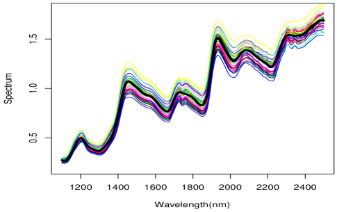
Figure D.1: Biscuit dough pieces data curves (thin solid lines) with their mean function estimator (thick solid line).

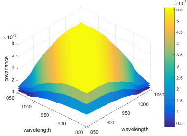
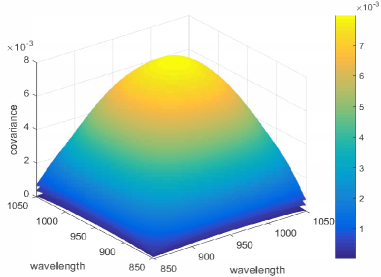
Figure D.2: Biscuit dough piece data plots: (a) covariance estimator $\widehat{G}^{\mathrm{PROP}}$ and its 95% SCE; (b) covariance estimator $\widehat{G}^{TPS}$ and its 95% SCE.

References

• Banerjee et al. (2004) Banerjee, S., Carlin, B., and Gelfand, A. (2004), Hierarchical Modeling and Analysis for Spatial Data, Boca Raton, FL: Chapman & Hall/CRC Press.
• Bosq (1998) Bosq, D. (1998), Nonparametric Statistics for Stochastic Processes: Estimation and Prediction, vol. 110, Springer-Verlag New York.
• Brown et al. (2001) Brown, P., Fearn, T., and Vannucci, M. (2001), “Bayesian wavelet regression on curves with application to a spectroscopic calibration problem,” J. Amer. Statist. Assoc., 96, 398–408.
• Cao et al. (2016) Cao, G., Wang, L., Li, Y., and Yang, L. (2016), “Oracle-efficient confidence envelopes for covariance functions in dense functional data,” Statist. Sinica, 26, 359–383.
• Cao et al. (2012) Cao, G., Yang, L., and Todem, D. (2012), “Simultaneous inference for the mean function based on dense functional data,” J. Nonparametr. Stat., 24, 359–377.
• Cardot (2000) Cardot, H. (2000), “Nonparametric estimation of smoothed principal components analysis of sampled noisy functions,” J. Nonparametr. Stat., 12, 503–538.
• Choi et al. (2013) Choi, I., Li, B., and Wang, X. (2013), “Nonparametric estimation of spatial and space-time covariance function,” J. Agric. Biol. Environ. Stat., 18, 611–630.
• Crainiceanu et al. (2009) Crainiceanu, C. M., Staicu, A. M., and Di, C. Z. (2009), “Generalized multilevel functional regression,” J. Amer. Statist. Assoc., 104, 1550–1561.
• Csörgo and Révész (1981) Csörgo, M. and Révész, P. (1981), Strong Approximations in Probability and Statistics, Academic Press, New York-London.
• de Boor (2001) de Boor, C. (2001), A Practical Guide to Splines, Springer, New York.
• Diggle and Verbyla (1998) Diggle, P. and Verbyla, A. (1998), “Nonparametric estimation of covariance structure in longitudinal data,” Biometrics, 54, 401–415.
• Ferraty and Vieu (2006) Ferraty, F. and Vieu, P. (2006), Nonparametric Functional Data Analysis: Theory and Practice. Springer Series in Statistics, Springer, Berlin.
• Fryzlewicz and Ombao (2009) Fryzlewicz and Ombao (2009), “Consistent classification of nonstationary time series using stochastic wavelet representations,” J. Amer. Statist. Assoc., 104, 299–312.
• Goldsmith et al. (2013) Goldsmith, J., Greven, S., and Crainiceanu, C. (2013), “Corrected confidence bands for functional data using principal components,” Biometrics, 69, 41–51.
• Guo et al. (2018) Guo, J., Zhou, B., and Zhang, J. T. (2018), “Testing the equality of several covariance functions for functional data: A supremum-norm based test,” Comput. Statist. Data Anal., 124, 15–26.
• Hall et al. (1994) Hall, P., Fisher, N. I., and Hoffmann, B. (1994), “On the nonparametric estimation of covariance functions,” Ann. Statist., 22, 2115–2134.
• Hall et al. (2006) Hall, P., Müller, H. G., and Wang, J. L. (2006), “Properties of Principal Component Methods for Functional and Longitudinal Data Analysis,” Ann. Statist., 34, 1493–1517.
• Horváth et al. (2013) Horváth, L., Kokoszka, P., and Reeder, R. (2013), “Estimation of the mean of functional time series and a two-sample problem,” J. R. Stat. Soc. Ser. B Stat. Methodol., 75, 103–122.
• Hsing and Eubank (2015) Hsing, T. and Eubank, R. (2015), Theoretical Foundations of Functional Data Analysis, with an Introduction to Linear operators. Wiley Series in Probability and Statistics, Wiley, Chichester.
• James et al. (2000) James, G., Hastie, T., and Sugar, C. (2000), “Principal component models for sparse functional data,” Biometrika, 87, 587–602.
• Li and Hsing (2010) Li, Y. and Hsing, T. (2010), “Uniform convergence rates for nonparametric regression and principal component analysis in functional/longitudinal data,” Ann. Statist., 38, 3321–3351.
• Olshen et al. (1989) Olshen, R. A., Biden, E. N., Wyatt, M. P., and Sutherland, D. H. (1989), “Gait Analysis and the Bootstrap,” Ann. Statist., 17, 1419–1440.
• Osborne et al. (1984) Osborne, B. G., Fearn, T., Miller, A. R., and Douglas, S. (1984), “Application of near infrared reflectance spectroscopy to the compositional analysis of biscuits and biscuit doughs,” J. Sci. Food Agric., 35, 99–105.
• Pantle et al. (2010) Pantle, U., Schmidt, V., and Spodarev, E. (2010), “On the estimation of integrated covariance functions of stationary random fields,” Scand. J. Statist., 37, 47–66.
• Peng and Paul (2009) Peng, J. and Paul, D. (2009), “A geometric approach to maximum likelihood estimation of the functional principal components from sparse longitudinal data,” Journal of Computational and Graphical Statistics, 18, 995–1015.
• Ramsay and Dalzell (1991) Ramsay, J. and Dalzell, C. (1991), “Some tools for functional data analysis,” J. R. Stat. Soc. Ser. B Stat. Methodol., 53, 539–572.
• Ramsay and Silverman (2005) Ramsay, J. and Silverman, B. (2005), Functional Data Analysis, Springer, New York.
• Sanderson et al. (2010) Sanderson, J., Fryzlewicz, P., and Jones, M. W. (2010), “Estimating linear dependence between nonstationary time series using the locally stationary wavelet model,” Biometrika, 97, 435–446.
• Song and Yang (2009) Song, Q. and Yang, L. (2009), “Spline confidence bands for variance functions,” J. Nonparametr. Stat., 21, 589–609.
• Tsyrulnikov and Gayfulin (2017) Tsyrulnikov, M. and Gayfulin, D. (2017), “A limited-area spatio-temporal stochastic pattern generator for simulation of uncertainties in ensemble applications,” Meteorologische Zeitschrift, 5, 549–566.
• Wang (2012) Wang, J. (2012), “Modelling time trend via spline confidence band,” Ann. Inst. Statist. Math., 64, 275–301.
• Wang and Yang (2009) Wang, J. and Yang, L. (2009), “Polynomial spline confidence bands for regression curves,” Statist. Sinica, 19, 325–342.
• Yang et al. (2016) Yang, J., Zhu, H., Choi, T., and Cox, D. D. (2016), “Smoothing and mean–covariance estimation of functional data with a Bayesian hierarchical model,” Bayesian Anal., 11, 649–670.
• Yao et al. (2005) Yao, F., Müller, H. G., and Wang, J. L. (2005), “Functional data analysis for sparse longitudinal data,” J. Amer. Statist. Assoc., 100, 577–590.
• Yin et al. (2010) Yin, J., Geng, Z., Li, R., and Wang, H. (2010), “Nonparametric covariance model,” Statist. Sinica, 20, 469–479.