High Precision Measurement of Compton Scattering in the 5 GeV region

Abstract

The cross section of atomic electron Compton scattering $\gamma+e\rightarrow\gamma^{\prime}+e^{\prime}$ was measured in the 4.400–5.475 GeV photon beam energy region by the PrimEx collaboration at Jefferson Lab with an accuracy of 2.6% and less. The results are consistent with theoretical predictions that include next-to-leading order radiative corrections. The measurements provide the first high precision test of this elementary QED process at beam energies greater than 0.1 GeV.

I I. Introduction

Quantum electrodynamics (QED) is one of the most successful theories in modern physics; and the Compton scattering of photons by free electrons $\gamma+e\rightarrow\gamma^{\prime}+e^{\prime}$ is the simplest and the most elementary pure QED process. The lowest-order Compton scattering diagrams (see Fig. 1) were first calculated by Klein and Nishina in 1929 Klein29 and by Tamm in 1930 Tamm30 . Higher-order contributions arising from the interference between the leading order single Compton scattering amplitude and the radiative and double Compton scattering amplitudes were calculated in the 1950s radiative1 ; Mandl52 . Figure 1 shows the Feynman diagrams illustrating these two processes. They were subsequently re-evaluated in the 60s and early 70s to make them amenable for calculation using modern computational techniques radiative2 -Ram71 . Corrections to the leading order Compton total cross section at the level of a few percent are predicted for beam energies above 0.1 GeV radiative3 , hence the next-to-leading order (NLO) corrections are important when studying Compton scattering at these energies.

Experiments performed so far were mostly in the energy region below 0.1 GeV; a few experiments probed the 0.1-1.0 GeV energy range with a precision of 10–15% Coensgen53 -Gittlman68 . Only one experiment Goshaw78 measured the Compton scattering total cross section up to 5.0 GeV using a bubble-chamber detection technique. The experimental uncertainties for energies above 1 GeV were at the level of 20–70%. Due to the lack of precise data, higher order corrections to the Klein-Nishina formula have never been tested experimentally. This paper reports on new measurements of the Compton scattering cross section with a precision of 1.7% performed by the PrimEx collaboration at Jefferson Lab (JLab) for two separate running periods. The total cross sections in a forward direction on ¹²C and ²⁸Si targets were measured in the 4.400–5.475 GeV-energy region. The precision achieved by this experiment provides, for the first time, an important test of the QED prediction for the Compton scattering process with corrections to the order of $\mathcal{O}$($\alpha$), where $\alpha$ is the fine structure constant. In this article, we will summarize the theoretical calculations (Sec. II), describe our experimental procedure (Sec. III), and present the results of the comparison between the data and the theoretical predictions (Sec. IV).

II II. A summary of theoretical calculations

The leading order Compton scattering cross section (see Fig. 1, top) was first calculated by Klein and Nishina Klein29 and the result is known as the Klein-Nishina formula Peskin95 :

$$\frac{d\sigma}{d\Omega}=\frac{r_{e}^{2}}{2}\frac{1}{[1+\gamma(1-\cos\theta)]^{2}}[1+\cos^{2}\theta+\frac{\gamma^{2}(1-\cos\theta)^{2}}{1+\gamma(1-\cos\theta)}]$$

where $r_{e}$ is the classical electron radius, $\gamma$ is the ratio of the photon beam energy to the mass of electron, and $\theta$ is the photon scattering angle. This formula predicts that the Compton scattering at high energies has two basic features: (i) the total cross section decreases with increasing beam energy, $E$, as approximately $1/E$, and (ii) the differential cross section is sharply peaked at small angles relative to the incident photons.

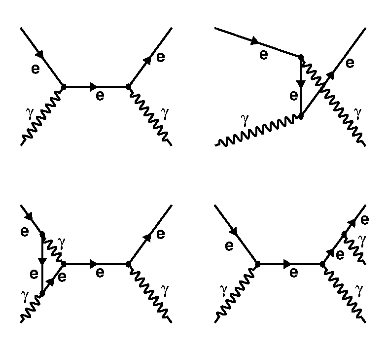
Figure 1: (Top) The lowest-order Feynman diagrams for single Compton scattering. (Bottom) Typical radiative correction (Left), and double Compton scattering contributions (Right) to single Compton scattering.

The theoretical foundation for the next-to-leading order radiative corrections to the Klein-Nishina formula had been well established by early 70s. The radiative corrections to $\mathcal{O}$($\alpha$) were initially evaluated by Brown and Feynman radiative1 in 1952. This correction is caused by two types of processes. The first type, a virtual-photon correction, arises from the possibility that the electron may emit and reabsorb a virtual photon in the scattering process (see bottom left panel of Fig. 1). The second type is a soft-photon double Compton effect, in which the energy of one of the emitted photons is much smaller than the electron mass ($\omega_{2}<\omega_{2max}\ll m_{e}$, where $\omega_{2}$ is the energy of the additional photon, $\omega_{2max}$ is a cut-off energy, and $m_{e}$ is the electron mass), as shown in the bottom right panel of Fig. 1. These two contributions must be taken into account together since it is impossible to separate them experimentally. Moreover, the infrared divergence term from the virtual-photon process is canceled by the infrared divergence term in the soft-photon double Compton process, resulting in a finite physically meaningful correction ($\delta^{SV}$). The value of $\delta^{SV}$, where $SV$ stands for $S$(oft) and $V$(irtual), is predicted to be negative as described by Eq. (2.6) and Eq. (2.15) in radiative3 .

On the other hand, a hard-photon double Compton effect occurs when both emitted photons in the double Compton process have energies larger than the cut-off energy, $\omega_{2max}$. When comparing the experimental result with the theoretical calculation, one must also take into account the contributions from the hard-photon double Compton effect since the experimental apparatus has finite resolutions leading to limitations on the measurements of both energies and angles radiative3 . The differential cross section of the double Compton effect was initially calculated by Mandl and Skyrme Mandl52 , and the total cross section of the Hard-photon Double Compton process ($\delta^{HD}$) is described by Eq. (6.6) in reference radiative3 and its value is predicted to be positive. Summing up $\delta^{SV}$ and $\delta^{HD}$, the total NLO correction to the total cross section is predicted to be a few percent for photon beam energies up to 10 GeV.

In order to interpret the experimental results and compare with the theoretical predictions, one needs to develop a reliable numerical method to integrate the cross section and calculate the radiative corrections incorporating the experimental resolutions. The latter is critical in calculating the contribution from the hard photon double Compton effect correctly. As discussed above, the corrections are divided into two types ($\delta^{SV}$ and $\delta^{HD}$) depending on whether the energy of the secondary emitted photon is less or greater than an arbitrary energy scale, denoted by $\omega_{2max}$, which should be much smaller than the electron mass radiative3 . Since the physically measurable cross section contains the corrections from both types, the final integrated total cross section must be independent of the values of $\omega_{2max}$. Two different methods had been developed to prove this independence.

The first method PrimEx42 is based on the BASES/SPRING Monte Carlo simulation package Kawabata . BASES uses the stratified sampling method to integrate the differential cross section, and SPRING uses the probability information obtained during the BASES integration to generate Compton events. The parameter $\omega_{2max}$ does not enter the differential cross section explicitly but is contained in the limits of integration over the energy. For a consistency check, the total cross section was calculated with several values of $\omega_{2max}$. While the calculated total Klein-Nishina cross section corrected with the virtual and soft photon processes ($\sigma_{SV}$) as well as the total hard photon double Compton cross section ($\sigma_{HD}$), both, depend on the $\omega_{2max}$ parameter, the sum of the two corrections ($\sigma_{SV}+\sigma_{HD}$) is independent, within 0.1%, of the choice of $\omega_{2max}$, as expected.

The second numerical method was developed by M. Konchatnyi PrimEx37 , where the parameter $\omega_{2max}$ is analytically removed from the integration. The total Compton scattering cross section on ¹²C along with radiative corrections, calculated using the two numerical methods PrimEx42  PrimEx37 described above, were compared to each other and to the XCOM Berger database of the National Institute of Standards and Technology (NIST). The cross sections were found to be consistent with each other. The radiative corrections are about 4% of the total cross section for a beam energy of $\sim$5 GeV. In the data analysis described below, the BASES/SPRING method is used to calculate the radiatively corrected cross section and to generate events for the experimental acceptance study.

III III. Experimental Procedure

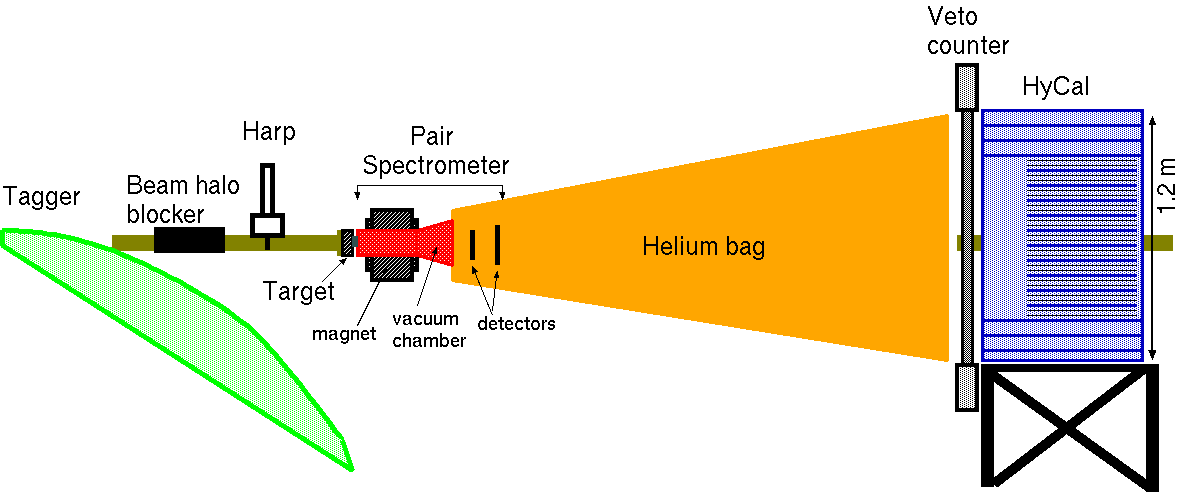
Figure 2: Diagram, not to scale, of the experimental setup. The pair spectrometer placed between the target and the helium bag, had the magnet turned off during the Compton experiment.

The atomic electron Compton scattering process $\gamma+e\rightarrow\gamma^{{}^{\prime}}+e^{\prime}$ was measured using the apparatus built for the PrimEx experiment ConceptualD , which aimed to measure the $\pi^{0}$ lifetime and was performed over two run periods in 2004 and 2010, in Hall B at JLab. The Compton scattering data were collected periodically, once per week during both running periods. The primary experimental equipment included (see Fig. 2): (i) the existing Hall B high intensity and high resolution photon tagger Sober , which provides the timing and energy information of incident photons up to 6 GeV; (ii) solid production targets Martel : ¹²C (5% radiation length (r.l.)), used during the first running period, and ¹²C (8% r.l.) and ²⁸Si (10% r.l.) added in the second running period; (iii) a pair spectrometer (PS), located downstream of the production target, to continuously measure the relative photon tagging ratio Teymurazyan , and consequently the absolute photon flux, which was obtained by normalizing to the absolute photon tagging efficiency measured periodically with a total absorption counter (TAC) at low beam intensities (not shown in Fig. 2); (iv) a $118\times 118$ cm² high resolution hybrid calorimeter (HyCal Gasparian ) with 12 scintillator charge particle veto counters, which were located $\sim$7 m downstream of the target, to detect forward scattered electromagnetic particles; and (v) a scintillator fiber based photon beam profile and position detector located behind HyCal for online beam position monitoring (not shown in Fig. 2).

To minimize the photon conversion and electron multiple scattering, the gap between the PS magnet and the HyCal was occupied by a plastic foil container filled with helium at atmospheric pressure. The energies and positions of the scattered photon and electron were measured by the HyCal calorimeter. In conjunction with the beam energy (4.9-5.5 GeV during the first experiment and 4.4-5.3 GeV during the second one), which was measured by the photon tagger, the complete kinematics of the Compton events was determined. During the Compton runs the experimental setup was identical to the one used for the $\pi^{0}$ production runs, except for the pair spectrometer magnet being turned off to allow detection of both scattered photons and recoiling electrons in the calorimeter. The use of the same experimental apparatus, as well as the similar kinematics allowed the measurement of the Compton cross section to be employed as a tool to verify the systematic uncertainty of the $\pi^{0}$ experiments. The photon flux, target thickness and HyCal energy response being some of the common systematic uncertainty between the Compton and $\pi^{0}$ run types and resulting analyses.

A coincidence between the photon tagger in the energy interval of 4.4–5.5 GeV and the HyCal calorimeter with a total energy deposition greater than 2.5 GeV formed an event trigger for the first running period, while in the second running period the trigger was defined just by the total energy deposition greater than 2.5 GeV in the HyCal. The event selection criteria were: (i) the time difference between the incident photon, $\rm{t_{Tag}}$ and the scattered particles detected by the HyCal calorimeter, $\rm{t_{HyCal}}$ had to be $|\rm{t_{Tag}-t_{HyCal}}|<5\sigma_{t}$, where $\sigma_{t}$ =1.03 ns is the timing resolution of the detector system. (ii) the difference in the azimuthal angle between the scattered photon and electron had to be $|\Delta\phi|<5\sigma_{\phi}$, where $\sigma_{\phi}=$7^∘ is the azimuthal angular resolution for the first running period, (for the second running period a target dependent resolution of $\sigma_{\phi}=$4.0 - 4.7^∘ was used); (iii) the reconstructed reaction vertex position was required to be consistent with the target thickness and position; (iv) the spatial distance between the scattered photon and electron as detected by the HyCal calorimeter had to be larger than a photon energy dependent minimum separation resulting from the reaction being elastic; the minimum separation of 16 cm for the first running period and $R_{min}(E)=$19.0 - 1.95$\times$(4.85-$E$) for the second running period; and (v) the difference between the incident photon energy as measured by the tagger, $\rm{E_{Tag}}$ and the reconstructed incident photon energy, $\rm{E_{HyCal}}$, had to be $|\rm{E_{Tag}-E_{HyCal}}|<$1 (0.4) GeV for the first (second) running period. In the event reconstruction, the measured energy of the more energetic scattered particles (photon or electron) and the coordinate information of both scattered particles detected by the calorimeter was used. The offline energy detection threshold per particle in the HyCal calorimeter was 0.5 GeV.

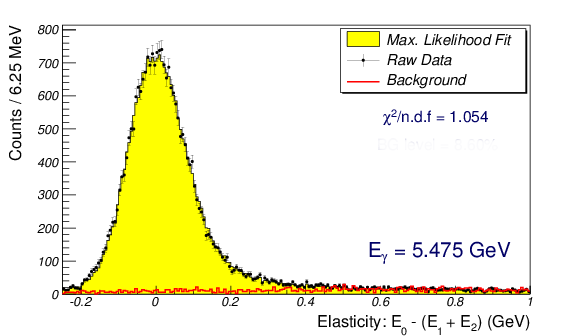
Figure 3: An example of the fit to the elasticity distribution for the highest energy bin. The background contribution is shown in red. $E_{0}$, $E_{1}$ + $E_{2}$ are the beam and sum of scattered electron and scattered $\gamma$ energies respectively. Note that since particle identification was not used, the photons and electrons cannot be distinguished from each other. The cluster with higher energy is designated as $E_{1}$ and the cluster with lower energy is designated as $E_{2}$.

To extract the Compton yields, the signal and background events (at a level of several percent of the yield) were separated for every incident photon energy bin (with a width of $\sim$1% of the nominal beam energy). The background originating from the target ladder and housing was determined using data from dedicated empty target runs, and the yields from these runs were normalized to the beam current and subtracted away. The remaining events that passed all of the five selection criteria described above were used to form an elasticity distribution, $\Delta E=E_{0}-(E_{1}+E_{2})$ where $E_{0}$ is the measured energy of the incident photon, and $E_{1}+E_{2}=E_{\gamma^{\prime}}+E_{e^{\prime}}$ is the sum of the scattered photon ($E_{\gamma^{\prime}}$) and the scattered electron ($E_{e^{\prime}}$) energies, which were either measured (the first experiment) or calculated using the Compton scattering kinematics (the second experiment). The cluster with higher energy is designated as $E_{1}$ and the cluster with lower energy is designated as $E_{2}$. The elasticity distribution was then fit to the simulated signal and background distributions, using a maximum likelihood method Barlow . Their overall amplitudes were parameters in the fit, as shown in Fig. 3, which is a typical result. The reduced $\chi^{2}$ for the different energy bins and for the 3 targets varied between 0.9 - 1.7.

The signal was generated by a Monte Carlo simulation employing the BASES/SPRING package as described in Sec. II PrimEx42 ,Kawabata , which included the radiative processes and the double Compton contribution. The simulated signal events were propagated through a GEANT-based simulation of the experimental apparatus and then processed using the same event reconstruction software that was used to extract the experimental yield. The GEANT based simulation framework includes parameters such as: light yield and transparency of PbWO₄ and lead-glass modules, the non-uniformity of the light yield (which was adjusted to match the light yield measured at IHEP, Protvino, Russia ilya ), and the quantum efficiency of the photo-multiplier tubes (Hamamatsu-R4125HA). The Monte Carlo parameters were tuned to reproduce the measured resolutions (position and energy) to within 3%, primarily for the calibration data obtained from the scan of the calorimeter with a tagged photon beam. The calibration scans were simulated to have the same statistics in the energy and position spectra as in the data, such that the uncertainty in the calibration constants for the data and simulation were the same. The energy response function and angular resolution was further verified by comparing the simulation to dedicated data collected using a thin 0.5% r.l. Be target and was found to be consistent within 3% Gasparian2 .

The shape of the background was modeled by the accidental events alone for the first running period, while the pair production channel was also included for the second running period. The accidental background was selected from the data using the events that were outside the coincidence time window, from $|\rm{t_{Tag}-t_{HyCal}}|>5\sigma_{t}$, but satisfied the remaining four criteria described above. The pair production contribution was generated using the GEANT simulation toolkit with its results handled in the same manner as the experimental yield. The amplitude from the maximum likelihood fit was then used to subtract the background from the experimental yield for each incident photon energy bin, giving the Compton yield.

IV IV. Results

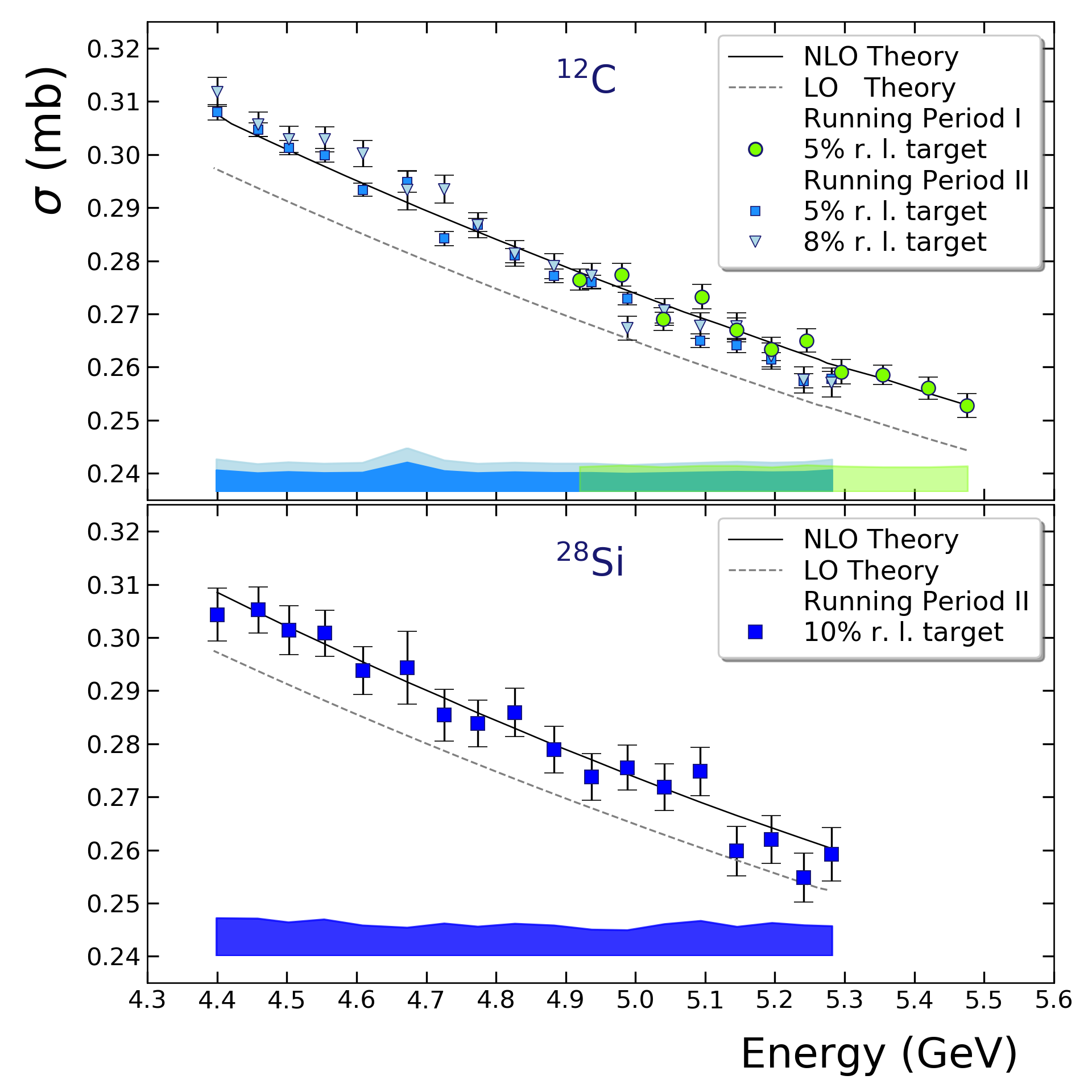
Figure 4: The Compton cross sections measured on atomic electrons of ¹²C and ²⁸Si targets. The dashed curve corresponds to the Klein-Nishina calculation. The solid curve is the result of next-to-leading order calculation. Error bars are statistical uncertainties. Bands at the bottom of both plots show point-to-point systematic uncertainties.

	Running Period
	I	II
Source Of Uncertainty	12C	12C(5%)	12C(8%)	28Si
photon flux	1.0	0.82	0.82	0.82
target composition, thickness	0.05	0.05	0.11	0.35
coincidence timing	0.05	0.49	0.68	0.60
coplanarity	0.08	0.51	0.66	0.71
geometrical acceptance	0.60	0.29	0.31	0.62
background subtraction	0.72	1.07	1.32	1.31
HyCal energy response	0.5	0.5	0.5	0.5
total	1.5	1.6	1.9	2.0

Table 1: Estimated systematic uncertainties, in percent, for each target over the entire energy range.

	12C - 5% r. l.			12C - 8% r. l.			28Si - 10% r. l.
Energy (GeV)	$\sigma$	$\delta_{stat}$	$\delta_{syst}$	$\sigma$	$\delta_{stat}$	$\delta_{syst}$	$\sigma$	$\delta_{stat}$	$\delta_{syst}$
4.40	0.3080	0.0014	0.0040	0.3118	0.0027	0.0062	0.3043	0.0050	0.0068
4.46	0.3047	0.0012	0.0039	0.3057	0.0023	0.0065	0.3052	0.0043	0.0068
4.50	0.3013	0.0013	0.0037	0.3029	0.0025	0.0051	0.3014	0.0046	0.0061
4.55	0.2999	0.0013	0.0043	0.3029	0.0024	0.0068	0.3008	0.0044	0.0066
4.61	0.2934	0.0013	0.0036	0.3002	0.0024	0.0053	0.2938	0.0045	0.0055
4.67	0.2949	0.0020	0.0046	0.2933	0.0037	0.0058	0.2943	0.0069	0.0051
4.73	0.2842	0.0014	0.0045	0.2935	0.0026	0.0051	0.2854	0.0049	0.0059
4.77	0.2868	0.0013	0.0047	0.2867	0.0024	0.0077	0.2838	0.0044	0.0053
4.83	0.2810	0.0013	0.0043	0.2814	0.0024	0.0039	0.2859	0.0046	0.0058
4.88	0.2772	0.0013	0.0063	0.2790	0.0024	0.0047	0.2789	0.0044	0.0055
4.92	0.2765	0.0020	0.0042
4.94	0.2760	0.0013	0.0059	0.2772	0.0024	0.0058	0.2738	0.0044	0.0048
4.98	0.2774	0.0021	0.0044
4.99	0.2729	0.0012	0.0059	0.2673	0.0022	0.0045	0.2755	0.0042	0.0047
5.04	0.2691	0.0021	0.0041
5.04	0.2691	0.0013	0.0033	0.2706	0.0023	0.0061	0.2718	0.0044	0.0058
5.09	0.2732	0.0023	0.0044
5.09	0.2650	0.0013	0.0045	0.2678	0.0024	0.0037	0.2748	0.0046	0.0063
5.15	0.2670	0.0023	0.0043
5.15	0.2641	0.0013	0.0047	0.2677	0.0025	0.0072	0.2598	0.0046	0.0053
5.20	0.2634	0.0022	0.0041
5.20	0.2614	0.0013	0.0035	0.2621	0.0024	0.0055	0.2620	0.0045	0.0060
5.24	0.2574	0.0013	0.0037	0.2576	0.0025	0.0054	0.2548	0.0046	0.0056
5.25	0.2650	0.0022	0.0045
5.28	0.2578	0.0014	0.0063	0.2571	0.0027	0.0040	0.2592	0.0050	0.0054
5.29	0.2591	0.0023	0.0042
5.36	0.2585	0.0018	0.0041
5.42	0.2560	0.0021	0.0041
5.47	0.2528	0.0022	0.0043

Table 2: Compton cross sections. Bold italicized numbers correspond to values obtained during the first running period.

The Compton scattering total cross sections (TABLE 2) were obtained by combining the extracted Compton yields with the luminosity and detector acceptance. Figure 4 shows the total Compton scattering cross sections from the first and the second running period, respectively as a function of the beam energy. The extracted cross sections are compared to a next-to-leading order calculation for both running periods. All the results agree with the theoretical calculations within the experimental uncertainties.

The average total systematic uncertainty for each data point is 1.5% for the first running period and is 1.6 - 2.0% for the second running period depending on the target (lowest for the 5% r.l. ¹²C target and highest for the 10% r.l. ²⁸Si target). The breakdown of the uncertainties is summarized in Table 1. The uncertainty in the photon flux is the largest source of uncertainty Teymurazyan . It was determined from the long term overall stability of the beam, data acquisition live time, and tagger false count rate. The uncertainty due to background subtraction was estimated from the variation in the fitting uncertainty with changes to the shape of the background distributions. The systematic uncertainty due to detector response was estimated from the change in experimental yield when the detector resolutions were varied by $\sim$3%. The geometrical acceptance uncertainty was estimated from the variation in the simulated yields with small changes to the experimental geometry. The target thickness uncertainty was 0.05% for the 5% r.l. ¹²C target. The uncertainty was higher for the thicker targets used during the second running period: 0.11% for the 8% r.l. ¹²C target and 0.35% for the 10% r.l. ²⁸Si target PrimEx74 .

The differences in systematic uncertainties for the two running periods stem from the differences in the experimental setup ( e.g. the geometry, the trigger ) and differences in data analysis ( e.g. the energy binning, event selection, and the background fits ).

V V. Conclusion

In conclusion, the total cross section for Compton scattering on ¹²C and ²⁸Si, in the 4.400 - 5.475 GeV-energy range was measured with the PrimEx experimental apparatus. The results are in excellent agreement with theoretical prediction with NLO radiative corrections. Averaged over all data points per target, the total uncertainties were 1.7% for the first running period, and 1.7%, 2.0%, and 2.6% for the second running period (for 5% r.l. and 8% r.l. ¹²C, and ²⁸Si targets, respectively - see Table 1). This measurement provides an important verification of the magnitude and the sign of the radiative effects in the Compton scattering, which was determined and separated from the leading order process for the first time. We conclude that this measurement constitutes the first confirmation that the QED next-to-leading order prediction correctly describes this fundamental process up to a photon energy, $E_{\gamma}$, of 5.5 GeV within our experimental precision.

VI VII. Acknowledgements

This work was funded in part by the U.S. Department of Energy, including contract AC05-06OR23177 under which Jefferson Science Associates, LLC operates Thomas Jefferson National Accelerator Facility, and by the U.S. National Science Foundation (NSF MRI PHY-0079840). We wish to thank the staff of Jefferson Lab for their vital support throughout the experiment. We are also grateful to all granting agencies providing funding support to authors throughout this project.

References

- (1) O. Klein and Y. Nishina, Z. Phys., 52, 853 (1929).
- (2) I. Tamm, Z. Phys., 62, 545 (1930).
- (3) I.M. Brown and R.P. Feynman, Phys. Rev., 85, 231(1952).
- (4) F. Mandl and T.H.R. Skyrme, Proc. R. Soc. London, A215, 497 (1952).
- (5) Till B. Anders, Nucl. Phys., 87, 721 (1967).
- (6) K.J. Mork, Phys. Rev., A4, 917 (1971).
- (7) M. Ram and P.Y. Wang, Phys. Rev. Lett., 26, 476 (1971);
- (8) A. Tkabladze, M. Konchatnyi, and Y. Prok, PrimEx Note 42, http://www.jlab.org/primex/.
- (9) S. Kawabata, Computer Physics Communications, 88, 309 (1995).
-
(10)
Mykhailo Konchatnyi, PrimEx Note 37,
http://www.jlab.org/primex/. - (11) M. Berger, et al., http://physics.nist.gov/xcom
-
(12)
Jefferson Lab experiments E-99-014 and E-02-103,
http://www.jlab.org/exp_prog/proposals/02/PR02-103.ps.
- (13) D. I. Sober et al., Nucl. Instrum. Meth. A 440, 263 (2000).
- (14) P. Martel et al., Nucl. Instrum. Meth. A 612, 46 (2009) ibid. 26, 1210(E)(1971).
- (15) A. Teymurazyan, Nucl. Instrum. Meth. A 767, 300 (2014)
- (16) A. Gasparian, Proc. of the XI Int’l Conf. On Calorimetry In Particle Physics, World Scientific, 109-115 (2004).
- (17) F. H. Coensgen, University of California Radiation Laboratory Report UCRL-2413, 1953 (unpublished).
- (18) L. V. Kurnosova et al., Zh. Eksp. Theor. Fiz., 30, 690 (1956) [Sov. Phys. - JETP 3, 546 (1956)].
- (19) J. D. Anderson et. al., Phys. Rev., 102, 1626 (1956).
- (20) B. Gittelman et. al., Phys. Rev., 171, 1388 (1968).
- (21) A.T. Goshaw et. al., Phys. Rev., D18, 1351 (1978).
- (22) M. Peskin and D. Schroeder, An Introduction to Quantum Field Theory, Addison-Wesley Publishing Company (1995).
- (23) R. Barlow, Computer Physics Communications, 77, 219 (1993).
- (24) I. Larin, PhD Thesis, ITEP, Moscow, (2014). https://www.jlab.org/primex/; V. Kravtsov private communications.
- (25) M. Kubantsev, I. Larin and A. Gasparian, Proc. of the XII Int’l Conf. On Calorimetry In Particle Physics, AIP Conference Proceedings 867, 51 (2006).
- (26) C. Harris, W. Barnes, and R. Miskimen, PrimEx Note 74, http://www.jlab.org/primex/.