EUROPEAN ORGANIZATION FOR NUCLEAR RESEARCH (CERN)

​​​ CERN-EP-2019-037 LHCb-PAPER-2019-003 6 August 2019

Measurement of the $C\!P$-violating phase $\phi_{s}$ from ${{B}^{0}_{s}}\rightarrow{{J\mskip-3.0mu/\mskip-2.0mu\psi\mskip 2.0mu}}\pi^{+}\pi^{-}$ decays in 13 TeV $pp$ collisions

LHCb collaboration

Decays of ${B}^{0}_{s}$ and ${\kern 1.79993pt\overline{\kern-1.79993ptB}}{}^{0}_{s}$ mesons into ${{J\mskip-3.0mu/\mskip-2.0mu\psi\mskip 2.0mu}}\pi^{+}\pi^{-}$ final states are studied in a data sample corresponding to 1.9 fb^-1 of integrated luminosity collected with the LHCb detector in 13 TeV $pp$ collisions. A time-dependent amplitude analysis is used to determine the final-state resonance contributions, the $C\!P$-violating phase $\phi_{s}=-0.057\pm 0.060\pm 0.011$ rad, the decay-width difference between the heavier mass ${B}^{0}_{s}$ eigenstate and the ${{B}^{0}}$ meson of $-0.050\pm 0.004\pm 0.004$ ps^-1, and the $C\!P$-violating parameter $|\lambda|=1.01_{-0.06}^{+0.08}\pm 0.03$, where the first uncertainty is statistical and the second systematic. These results are combined with previous LHCb measurements in the same decay channel using 7 TeV and 8 TeV $pp$ collisions obtaining $\phi_{s}=0.002\pm 0.044\pm 0.012$ rad, and $|\lambda|=0.949\pm 0.036\pm 0.019$.

Published in Phys. Lett. B797 (2019)

© 2024 CERN for the benefit of the LHCb collaboration. CC-BY-4.0 licence.

 

1 Introduction

Measurements of $C\!P$ violation in final states that can be populated both by direct decay and via mixing provide an excellent way of looking for physics beyond the Standard Model (SM) [1]. As yet unobserved heavy bosons, light bosons with extremely small couplings, or fermions can be present virtually in quantum loops, and thus affect the relative $C\!P$ phase. Direct decays into non-flavour-specific final states can interfere with those that undergo ${{B}^{0}_{s}}-{{\kern 1.79993pt\overline{\kern-1.79993ptB}}{}^{0}_{s}}$ mixing prior to decay. This interference can result in $C\!P$ violation. In certain ${B}^{0}_{s}$ decays one $C\!P$-violating phase that can be measured, called $\phi_{s}$, can be expressed in terms of Cabibbo-Kobayashi-Maskawa matrix elements as $-2{\arg}\left[{-V_{ts}V_{tb}^{*}}/{V_{cs}V_{cb}^{*}}\right]$. It is not predicted in the SM, but can be inferred with high precision from other experimental data giving a value of $-36.5_{-1.2}^{+1.3}$ mrad [2]. This number is consistent with previous measurements, which did not have enough sensitivity to determine a non-zero value [3, *Abazov:2008af, *CDF:2011af, *Abazov:2011ry, 7, 8, 9, 10, *Khachatryan:2015nza]. In this paper we present the results of a new analysis of the ${{B}^{0}_{s}}\rightarrow{{J\mskip-3.0mu/\mskip-2.0mu\psi\mskip 2.0mu}}\pi^{+}\pi^{-}$ decay using data from 13 TeV $pp$ collisions collected using the LHCb detector in 2015 and 2016. The existence of this decay and its use in $C\!P$-violation studies was suggested in Ref. [12].

2 Detector and simulation

The LHCb detector [13, 14] is a single-arm forward spectrometer covering the pseudorapidity range $2<\eta<5$, designed for the study of particles containing $b$ or $c$ quarks. The detector includes a high-precision tracking system consisting of a silicon-strip vertex detector surrounding the $pp$ interaction region [15], a large-area silicon-strip detector located upstream of a dipole magnet with a bending power of about $4{\mathrm{\,Tm}}$, and three stations of silicon-strip detectors and straw drift tubes placed downstream of the magnet. The tracking system provides a measurement of the momentum, $p$, of charged particles with a relative uncertainty that varies from 0.5% at low momentum to 1.0% at 200 GeV. The minimum distance of a track to a primary vertex (PV), the impact parameter (IP), is measured with a resolution of $(15+29/p_{\mathrm{T}})\,\upmu\text{m}$, where $p_{\mathrm{T}}$ is the component of the momentum transverse to the beam, in  GeV. Different types of charged hadrons are distinguished using information from two ring-imaging Cherenkov detectors [16]. Photons, electrons and hadrons are identified by a calorimeter system consisting of scintillating-pad and preshower detectors, an electromagnetic and a hadronic calorimeter. Muons are identified by a system composed of alternating layers of iron and multiwire proportional chambers [17]. The online event selection is performed by a trigger, which consists of a hardware stage, based on information from the calorimeter and muon systems, followed by a software stage, which applies a full event reconstruction.

At the hardware trigger stage, events are required to have a muon with high $p_{\mathrm{T}}$ or a hadron, photon or electron with high transverse energy in the calorimeters. The software trigger is composed of two stages, the first of which performs a partial reconstruction and requires either a pair of well-reconstructed, oppositely charged muons having an invariant mass above $2.7\text{\,Ge\kern-1.00006ptV}$, or a single well-reconstructed muon with $p_{\mathrm{T}}>1\text{\,Ge\kern-1.00006ptV}$ and have a large IP significance $\chi^{2}_{\text{IP}}>7.4$. The latter is defined as the difference in the $\chi^{2}$ of the vertex fit for a given PV reconstructed with and without the considered particles. The second stage applies a full event reconstruction and for this analysis requires two opposite-sign muons to form a good-quality vertex that is well-separated from all of the PVs, and to have an invariant mass within $\pm 120\text{\,Me\kern-1.00006ptV}$ of the known ${J\mskip-3.0mu/\mskip-2.0mu\psi\mskip 2.0mu}$ mass [18].

Simulation is required to model the effects of the detector acceptance and the imposed selection requirements. In the simulation, $pp$ collisions are generated using Pythia [19, *Sjostrand:2007gs] with a specific LHCb configuration [21]. Decays of unstable particles are described by EvtGen [22], in which final-state radiation is generated using Photos [23]. The interaction of the generated particles with the detector, and its response, are implemented using the Geant4 toolkit [24, *Agostinelli:2002hh] as described in Ref. [26].

3 Decay amplitude

The resonance structure in ${{B}^{0}_{s}}$ and ${{\kern 1.79993pt\overline{\kern-1.79993ptB}}{}^{0}_{s}}\rightarrow{{J\mskip-3.0mu/\mskip-2.0mu\psi\mskip 2.0mu}}\pi^{+}\pi^{-}$ decays has been previously studied with a time-integrated amplitude analysis using 7 and 8 TeV $pp$ collisions [27]. The final state was found to be compatible with being entirely $C\!P$-odd, with the $C\!P$-even state fraction below $2.3$% at 95% confidence level, which allows the determination of the decay width of the heavy ${{B}^{0}_{s}}$ mass eigenstate, ${\Gamma_{\mathrm{H}}}$. The possible presence of a $C\!P$-even component is taken into account when determining $\phi_{s}$ [28].

The total decay amplitude for a ( ) [-.7ex] $\kern-1.79993pt{{B}^{0}_{s}}$ meson at decay time equal to zero is assumed to be the sum over individual ${{\pi}^{+}}{{\pi}^{-}}$ resonant transversity amplitudes [29], and one nonresonant amplitude, with each transversity component labelled as ${A}_{i}$ ($\overline{A}_{i}$). Because of the spin-1 ${{J\mskip-3.0mu/\mskip-2.0mu\psi\mskip 2.0mu}}$ meson in the final state, the three possible polarizations of the ${{J\mskip-3.0mu/\mskip-2.0mu\psi\mskip 2.0mu}}$ generate longitudinal ($0$), parallel ($\parallel$) and perpendicular ($\perp$) transversity amplitudes. When the ${{\pi}^{+}}{{\pi}^{-}}$ pair forms a spin-0 state the final system only has a longitudinal component, and thus is a pure $C\!P$ eigenstate. The parameter $\lambda_{i}\equiv\frac{q}{p}\frac{\overline{A}_{i}}{A_{i}}$, relates $C\!P$ violation in the interference between mixing and decay associated with the polarization state $i$ for each resonance in the final state. Here the quantities $q$ and $p$ relate the mass and flavour eigenstates, $p\equiv\langle{{B}^{0}_{s}}|B_{\rm L}\rangle$, and $q\equiv\langle{{\kern 1.79993pt\overline{\kern-1.79993ptB}}{}^{0}_{s}}|B_{\rm L}\rangle$, where $|B_{\rm L}\rangle$ is the lighter mass eigenstate [1]. The total amplitudes ${\cal A}$ and $\overline{{\cal A}}$ can be expressed as the sums of the individual ( ) [-.7ex] $\kern-1.79993pt{{B}^{0}_{s}}$ amplitudes, ${\cal A}=\sum A_{i}$ and $\overline{{\cal A}}=\sum\frac{q}{p}\overline{A}_{i}=\sum\lambda_{i}A_{i}=\sum\eta_{i}|\lambda_{i}|e^{-i\phi_{s}^{i}}A_{i}$, with $\eta_{i}$ being the $C\!P$ eigenvalue of the state. For each transversity state $i$ there is a $C\!P$-violating phase $\phi_{s}^{i}\equiv-\arg(\eta_{i}\lambda_{i})$ [30]. Assuming that $C\!P$ violation in the decay is the same for all amplitudes, then $\lambda\equiv\eta_{i}\lambda_{i}$ and $\phi_{s}\equiv-\arg(\lambda)$. Using $|p/q|=1$, the decay rates for ${{B}^{0}_{s}}$ and ${{\kern 1.79993pt\overline{\kern-1.79993ptB}}{}^{0}_{s}}$ into the ${{J\mskip-3.0mu/\mskip-2.0mu\psi\mskip 2.0mu}}{{\pi}^{+}}{{\pi}^{-}}$ final state are

$$\kern 1.79993pt\shortstack{{(\rule[2.15277pt]{12.50002pt}{0.51212pt})} \\ [-.7ex] $\kern-1.79993pt\Gamma$}(t)\propto e^{-{\Gamma_{{s}}}t}\left\{\frac{|{\cal A}|^{2}+|\overline{{\cal A}}|^{2}}{2}\cosh\frac{{\Delta\Gamma_{{s}}}t}{2}\pm\frac{|{\cal A}|^{2}-|\overline{{\cal A}}|^{2}}{2}\cos({\Delta m_{{s}}}t)\right.\quad\quad$$

$$-\left.\mathcal{R}e({\cal A}^{*}\overline{{\cal A}})\sinh\frac{{\Delta\Gamma_{{s}}}t}{2}\mp\mathcal{I}m({\cal A}^{*}\overline{{\cal A}})\sin({\Delta m_{{s}}}t)\right\},$$ (1)

where the – sign before the $\cos({\Delta m_{{s}}}t)$ term and $+$ sign before the $\sin({\Delta m_{{s}}}t)$ term apply to $\overline{\Gamma}(t)$, ${\Delta\Gamma_{{s}}}\equiv{\Gamma_{\mathrm{L}}}-{\Gamma_{\mathrm{H}}}$ is the decay-width difference between the light and the heavy mass eigenstates, ${\Delta m_{{s}}}\equiv m_{\rm H}-m_{\rm L}$ is the corresponding mass difference, and ${\Gamma_{{s}}}\equiv({\Gamma_{\mathrm{L}}}+{\Gamma_{\mathrm{H}}})/2$ is the average ${{B}^{0}_{s}}$ meson decay width [32].

For ${{J\mskip-3.0mu/\mskip-2.0mu\psi\mskip 2.0mu}}$ decays to $\mu^{+}\mu^{-}$ final states the $A_{i}$ amplitudes are themselves functions of four variables: the ${{\pi}^{+}}{{\pi}^{-}}$ invariant mass $m_{\pi\pi}$, and three angular variables $\Omega\equiv(\cos\theta_{\pi\pi},\cos\theta_{{{J\mskip-3.0mu/\mskip-2.0mu\psi\mskip 2.0mu}}},\chi)$, defined in the helicity basis. These angles are defined as $\theta_{\pi\pi}$ between the $\pi^{+}$ direction in the ${{\pi}^{+}}{{\pi}^{-}}$ rest frame with respect to the ${{\pi}^{+}}{{\pi}^{-}}$ direction in the ${{B}^{0}_{s}}$ rest frame, $\theta_{{{J\mskip-3.0mu/\mskip-2.0mu\psi\mskip 2.0mu}}}$ between the $\mu^{+}$ direction in the ${{J\mskip-3.0mu/\mskip-2.0mu\psi\mskip 2.0mu}}$ rest frame with respect to the ${{J\mskip-3.0mu/\mskip-2.0mu\psi\mskip 2.0mu}}$ direction in the ${{B}^{0}_{s}}$ rest frame, and $\chi$ between the ${{J\mskip-3.0mu/\mskip-2.0mu\psi\mskip 2.0mu}}$ and ${{\pi}^{+}}{{\pi}^{-}}$ decay planes in the ${{B}^{0}_{s}}$ rest frame [28, 30]. (These definitions are the same for $B_{s}^{0}$ and $\overline{B}{}_{s}^{0}$, namely, using $\mu^{+}$ and $\pi^{+}$ to define the angles for both $B_{s}^{0}$ and $\overline{B}{}_{s}^{0}$ decays.) The explicit forms of the $|{\cal A}(m_{\pi\pi},\Omega)|^{2}$, $|\overline{{\cal A}}(m_{\pi\pi},\Omega)|^{2}$, and ${\cal A}^{*}(m_{\pi\pi},\Omega)\overline{{\cal A}}(m_{\pi\pi},\Omega)$ terms in Eq. (3) are given in Ref. [28].

The analysis proceeds by performing an unbinned maximum-likelihood fit to the ${\pi}^{+}$ ${\pi}^{-}$ mass distribution, the decay time, and helicity angles of ${B}^{0}_{s}$ candidates identified as ${B}^{0}_{s}$ or ${\kern 1.79993pt\overline{\kern-1.79993ptB}}{}^{0}_{s}$ by a flavour-tagging algorithm [33, *Aaij:2016psi, *Fazzini:2018dyq]. The fit provides the $C\!P$-even and $C\!P$-odd components, and since we include the initial flavour tag, the fit also determines the $C\!P$-violating parameters ${\phi_{{s}}}$ and $|\lambda|$, and the decay width. In order to proceed, we need to select a clean sample of ${B}^{0}_{s}$ decays, determine acceptance corrections, perform a calibration of the decay-time resolution in each event as a function of its uncertainty, and calibrate the flavour-tagging algorithm.

4 Selection requirements

The selection of ${{J\mskip-3.0mu/\mskip-2.0mu\psi\mskip 2.0mu}}{{\pi}^{+}}{{\pi}^{-}}$ right-sign (RS), and wrong-sign (WS) ${{J\mskip-3.0mu/\mskip-2.0mu\psi\mskip 2.0mu}}{{\pi}^{\pm}}{{\pi}^{\pm}}$ final states, proceeds in two phases. Initially we impose loose requirements and subsequently use a multivariate analysis to further suppress the combinatorial background. In the first phase we require that the ${J\mskip-3.0mu/\mskip-2.0mu\psi\mskip 2.0mu}$ decay tracks be identified as muons, have $p_{\mathrm{T}}>500\text{\,Me\kern-1.00006ptV}$, and form a good vertex with vertex fit $\chi^{2}$ less than 16. The identified pions are required to have $p_{\mathrm{T}}>250\text{\,Me\kern-1.00006ptV}$, not originate from any PV, and form a good vertex with the muons. The resulting ${B}^{0}_{s}$ candidate is assigned to the PV for which it has the smallest $\chi^{2}_{\text{IP}}$. Furthermore, we require that the smallest $\chi^{2}_{\text{IP}}$ is not greater than 25. The ${B}^{0}_{s}$ candidate is required to have its momentum vector aligned with the vector connecting the PV to the ${B}^{0}_{s}$ decay vertex, and to have a decay time greater than 0.3 ps. Reconstructed tracks sharing the same hits are vetoed.

In addition, background from ${{{B}^{+}}}\rightarrow{{J\mskip-3.0mu/\mskip-2.0mu\psi\mskip 2.0mu}}K^{+}$ decays, where the $K^{+}$ is misidentified as a $\pi^{+}$ and combined with a random $\pi^{-}$, is vetoed by assuming that each detected pion is a kaon, computing the ${{J\mskip-3.0mu/\mskip-2.0mu\psi\mskip 2.0mu}}{{K}^{+}}$ mass, and removing those candidates that are within $\pm 36$ MeV of the known ${{B}^{+}}$ mass [18]. Backgrounds from ${{B}^{0}}\rightarrow{{J\mskip-3.0mu/\mskip-2.0mu\psi\mskip 2.0mu}}K^{+}\pi^{-}$ or ${{B}^{0}_{s}}\rightarrow{{J\mskip-3.0mu/\mskip-2.0mu\psi\mskip 2.0mu}}K^{+}K^{-}$ decays with misidentified kaons result in masses lower than the ${B}^{0}_{s}$ peak and thus do not need to be vetoed.

For the multivariate part of the selection, we use a Boosted Decision Tree, BDT [36, 37], with the uBoost algorithm [38]. The algorithm is optimized to not further bias acceptance on the variable $\cos\theta_{\pi\pi}$. The variables used to train the BDT are the difference between the muon and pion identifications for the muon identified with lower quality, the $p_{\mathrm{T}}$ of the ${{B}^{0}_{s}}$ candidate, the sum of the $p_{\mathrm{T}}$ of the two pions, and the natural logarithms of: the $\chi^{2}_{\text{IP}}$ of each of the pions, the $\chi^{2}$ of the ${{B}^{0}_{s}}$ vertex and decay tree fits [39], and the $\chi^{2}_{\text{IP}}$ of the ${{B}^{0}_{s}}$ candidate. In the fit, the ${B}^{0}_{s}$ momentum vector is constrained to point to the PV, the two muons are constrained to the ${J\mskip-3.0mu/\mskip-2.0mu\psi\mskip 2.0mu}$ mass, and all four tracks are constrained to originate from the same vertex.

Implementing uBoost requires a training procedure. Data background in the ${{J\mskip-3.0mu/\mskip-2.0mu\psi\mskip 2.0mu}}\pi^{+}\pi^{-}$ mass interval between 200 to 250 MeV above the ${{B}^{0}_{s}}$ mass and simulated signal are first used. Then, separate samples are used to test the BDT performance. We weight the training simulation samples to match the two-dimensional ${{B}^{0}_{s}}$ $p$ and $p_{\mathrm{T}}$ distributions, and smear the vertex fit $\chi^{2}$, to match the background-subtracted preselected data. Finally, the minimum requirement for BDT point is chosen to maximize signal significance, $S/\sqrt{S+B}$, where $S(B)$ is the expected signal (background) yields in a range corresponding to $\pm 2.5$ times the mass resolution around the known ${{B}^{0}_{s}}$ mass [18].

To determine the signal and background yields we fit the candidate ${B}^{0}_{s}$ mass distribution. Backgrounds include combinatorics, whose shape is estimated using WS ${{J\mskip-3.0mu/\mskip-2.0mu\psi\mskip 2.0mu}}\pi^{\pm}\pi^{\pm}$ candidates modelled by an exponential function, ${{B}^{0}_{s}}\rightarrow{{J\mskip-3.0mu/\mskip-2.0mu\psi\mskip 2.0mu}}\eta^{\prime}(\rightarrow\rho^{0}\gamma)$ decays with the $\gamma$ ignored, and ${{\mathchar 28931\relax}^{0}_{b}}\rightarrow{{J\mskip-3.0mu/\mskip-2.0mu\psi\mskip 2.0mu}}p{{K}^{-}}$ decays with both hadrons misidentified as pions. The latter backgrounds are modelled using simulation. The ${{B}^{0}_{s}}$ signal shape is parameterized by a Hypatia function [40], where the signal radiative tail parameters are fixed to values obtained from simulation. The same shape parameters are used for the ${{B}^{0}}\rightarrow{{J\mskip-3.0mu/\mskip-2.0mu\psi\mskip 2.0mu}}\pi^{+}\pi^{-}$ decays, with the mean value shifted by the known ${B}^{0}_{s}$ and ${B}^{0}$ meson mass difference [18]. Finally, we fit simultaneously both RS and WS candidates, using the simulated shape for ${{B}^{0}_{s}}\rightarrow{{J\mskip-3.0mu/\mskip-2.0mu\psi\mskip 2.0mu}}\eta^{\prime}(\rightarrow\rho^{0}\gamma)$ whose yield is allowed to float, and fixing both the size and shape of the ${{\mathchar 28931\relax}^{0}_{b}}\rightarrow{{J\mskip-3.0mu/\mskip-2.0mu\psi\mskip 2.0mu}}p{{K}^{-}}$ component. The results of the fit are shown in Fig. 1. We find $33\,530\pm 220$ signal ${B}^{0}_{s}$ within $\pm 20$ MeV of the ${{B}^{0}_{s}}$ mass peak, with a purity of 84%. These decays are used for further analysis. Multiple candidates in the same event have a rate of 0.20% in a $\pm 20$ MeV interval around the ${{B}^{0}_{s}}$ mass peak, and are retained.

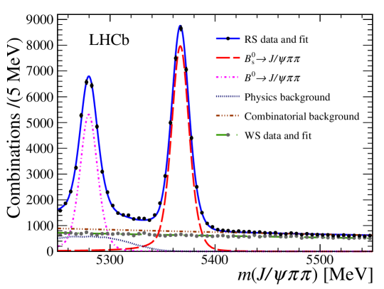
Figure 1: Results of the simultaneous fit to the ${{J\mskip-3.0mu/\mskip-2.0mu\psi\mskip 2.0mu}}\pi\pi$ mass distributions RS (black points) and WS (grey points) samples. The solid (blue) curve shows the fit to the RS sample, the long dashed (red) curve shows the signal, the dot-dashed (magenta) curve shows ${{B}^{0}}\rightarrow{{J\mskip-3.0mu/\mskip-2.0mu\psi\mskip 2.0mu}}{{\pi}^{+}}{{\pi}^{-}}$ decays, the dot-long-dashed (brown) curve shows the combinatorial background, the dotted (black) curve shows the sum of ${{B}^{0}_{s}}\rightarrow{{J\mskip-3.0mu/\mskip-2.0mu\psi\mskip 2.0mu}}\eta^{\prime}$ and ${{\mathchar 28931\relax}^{0}_{b}}$ background, while the dot-dot-dashed (green) curve shows the fit to WS sample.

To subtract the background in the signal region in the amplitude fit we add negatively weighted events from the WS sample to the RS sample, also accounting for the differing $\pi\pi$ mass and decay-time distributions. The weights are determined by comparing the RS and WS mass distributions in the upper mass sideband ($5420-5550\text{\,Me\kern-1.00006ptV}$). In addition, a small component of ${{B}^{0}_{s}}\rightarrow{{J\mskip-3.0mu/\mskip-2.0mu\psi\mskip 2.0mu}}\eta^{\prime}(\eta^{\prime}\rightarrow\rho^{0}\gamma)$ decays is also subtracted, since it is absent in the WS sample.

5 Detector efficiency and resolution

The correlated efficiencies in $m_{\pi\pi}$ and angular variables $\Omega$ are determined from simulation. We weight the simulated signal events to reproduce the ${B}^{0}_{s}$ meson $p_{\mathrm{T}}$ and $\eta$ distributions as well as the track multiplicity of the events. The latter may influence the efficiencies of the tracking and particle identification. The calculated efficiencies are shown in Fig. 2 along with the determined efficiency function.

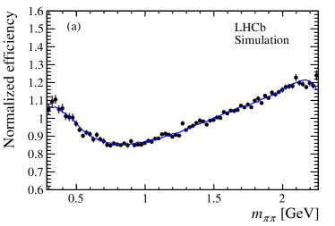
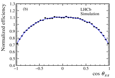
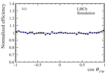
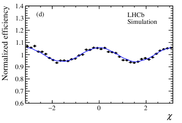
Figure 2: Overall efficiency normalized to unity for (a) $m_{\pi\pi}$ , (b) $\cos\theta_{\pi\pi}$ , (c) $\cos\theta_{{{J\mskip-3.0mu/\mskip-2.0mu\psi\mskip 2.0mu}}}$ and (d) $\chi$ observables. The points with error bars are from the ${{B}^{0}_{s}}\rightarrow{{J\mskip-3.0mu/\mskip-2.0mu\psi\mskip 2.0mu}}{{\pi}^{+}}{{\pi}^{-}}$ simulation, while the curves show the projection of the efficiency function.

The four-dimensional efficiency is parameterized by a combination of Legendre and spherical harmonic moments [41], as

$$\varepsilon(m_{\pi\pi},\cos\theta_{\pi\pi},\cos\theta_{{{J\mskip-3.0mu/\mskip-2.0mu\psi\mskip 2.0mu}}},\chi)=\sum_{a,b,c,d}\epsilon^{abcd}P_{a}(\cos\theta_{\pi\pi})Y_{bc}(\theta_{{{J\mskip-3.0mu/\mskip-2.0mu\psi\mskip 2.0mu}}},\chi)P_{d}\left(2\frac{m_{\pi\pi}-m_{\pi\pi}^{\rm min}}{m_{\pi\pi}^{\rm max}-m_{\pi\pi}^{\rm min}}-1\right),$$ (2)

where $P_{a}$ and $P_{d}$ are Legendre polynomials, $Y_{bc}$ are spherical harmonics, $m_{\pi\pi}^{\rm min}=2m_{\pi^{+}}$ and $m_{\pi\pi}^{\rm max}=m_{{{B}^{0}_{s}}}-m_{{{J\mskip-3.0mu/\mskip-2.0mu\psi\mskip 2.0mu}}}$, and $\epsilon^{abcd}$ are efficiency coefficients determined from weighted averages of decays generated uniformly over phase space [9].

The model gives an excellent representation of the simulated data. The efficiency is uniform within about $\pm 4$% for $\cos\theta_{{{J\mskip-3.0mu/\mskip-2.0mu\psi\mskip 2.0mu}}}$ and about 10% for $\chi$ variables; however the $m_{\pi\pi}$ and $\cos\theta_{\pi\pi}$ variables show large efficiency variations and correlations (see Fig. 3), due to the $\chi^{2}_{\text{IP}}$ $>\ 4$ requirements on the hadrons. The loss of efficiency in the lower $m_{\pi\pi}$ region can be interpreted as the projection of the effects of cuts on $\chi^{2}_{\text{IP}}$. Events at $\cos\theta_{\pi\pi}=\pm 1$ and $m_{\pi\pi}\simeq 0.6-0.8$ GeV are at the kinematic boundary of $m^{2}_{{{J\mskip-3.0mu/\mskip-2.0mu\psi\mskip 2.0mu}}\pi^{+}}$. One of the pions is almost at rest in ${{B}^{0}_{s}}$ rest frame, and thus the pion points to the PV, resulting in a very small $\chi^{2}_{\text{IP}}$ for this pion. The $\chi^{2}_{\text{IP}}$ variable is the most useful tool to suppress large pion combinatorial background from the PV.

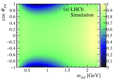
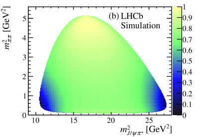
Figure 3: Overall efficiency for (a) $m_{\pi\pi}$ vs $\cos\theta_{\pi\pi}$ and (b) $m^{2}_{{{J\mskip-3.0mu/\mskip-2.0mu\psi\mskip 2.0mu}}{{\pi}^{+}}}$ vs $m^{2}_{\pi\pi}$. The inefficiency is at the kinematic boundary of $m^{2}_{{{J\mskip-3.0mu/\mskip-2.0mu\psi\mskip 2.0mu}}\pi^{+}}$ where the pion is almost at rest in the ${B}^{0}_{s}$ frame.

The reconstruction efficiency is not constant as a function of ${B}^{0}_{s}$ decay time due to displacement requirements applied to the hadrons in the offline selections and on ${{J\mskip-3.0mu/\mskip-2.0mu\psi\mskip 2.0mu}}$ candidates in the trigger. It is determined using the control channel ${{B}^{0}}\rightarrow{{J\mskip-3.0mu/\mskip-2.0mu\psi\mskip 2.0mu}}{K}^{*}(892)^{0}$, with ${K}^{*}(892)^{0}\rightarrow{{K}^{+}}{{\pi}^{-}}$, which is known to have a lifetime of $\tau_{{{B}^{0}}}=1.520\pm 0.004\text{\,ps}$ [18]. The simulated ${B}^{0}$ events are weighted to reproduce the distributions in the data for $p_{\mathrm{T}}$ and $\eta$ of the ${B}^{0}$ meson, and the invariant mass and helicity angle of ${K}^{+}$ ${\pi}^{-}$ system, as well as the track multiplicity of the events. The signal efficiency is calculated as $\varepsilon_{\rm data}^{{{B}^{0}_{s}}}(t)=\varepsilon_{\rm data}^{{{B}^{0}}}(t)\cdot{\varepsilon_{\rm sim}^{{{B}^{0}_{s}}}(t)}/{\varepsilon_{\rm sim}^{{{B}^{0}}}(t)}$, where $\varepsilon_{\rm data}^{{{B}^{0}}}(t)$ is the efficiency of the control channel as measured by comparing data with the known lifetime distribution, and $\varepsilon_{\rm sim}^{{{B}^{0}_{s}}}(t)/\varepsilon_{\rm sim}^{{{B}^{0}}}(t)$ is the ratio of efficiencies of the simulated signal and control mode after the full trigger and selection chain have been applied. This correction accounts for the small differences in the kinematics between the signal and control modes. The details of the method are explained in Ref. [7].

The acceptance is checked by measuring the decay width of ${{{B}^{+}}}\rightarrow{{J\mskip-3.0mu/\mskip-2.0mu\psi\mskip 2.0mu}}K^{+}$ decays. The fitted decay-width difference between the ${{{B}^{+}}}$ and ${{B}^{0}}$ mesons is $\Gamma_{{{{B}^{+}}}}-\Gamma_{{{B}^{0}}}=-0.0475\pm 0.0013$$\text{\,ps}^{-1}$, where the uncertainty is statistical only, in agreement with the known value of $-0.0474\pm 0.0023$$\text{\,ps}^{-1}$ [18].

From the measured ${B}^{0}_{s}$ candidate momentum and decay distance, the decay time and its event-by-event uncertainty $\delta_{t}$ are calculated. The calculated uncertainty is imbedded into the resolution function, which is modelled by the sum of three Gaussian functions with common means and widths proportional to a quadratic function of $\delta_{t}$. The parameters of the resolution function are determined with a sample of putative prompt ${{J\mskip-3.0mu/\mskip-2.0mu\psi\mskip 2.0mu}}\rightarrow\mu^{+}\mu^{-}$ decays combined with two pions of opposite charge. Taking into account the decay-time uncertainty distribution of the ${B}^{0}_{s}$ signal, the average effective resolution is found to be 41.5 fs. The method is validated using simulation; we estimate the accuracy of the resolution determination to be $\pm$3%.

6 Flavour tagging

Knowledge of the ( ) [-.7ex] $\kern-1.79993pt{{B}^{0}_{s}}$ flavour at production is necessary. We use information from decays of the other $b$ hadron in the event (opposite-side, OS) and fragments of the jet that produced the ( ) [-.7ex] $\kern-1.79993pt{{B}^{0}_{s}}$ meson that contain a charged kaon, called same-side kaon (SSK) [33, *Aaij:2016psi, *Fazzini:2018dyq]. The OS tagger infers the flavour of the other $b$ hadron in the event from the charges of muons, electrons, kaons, and the net charge of the particles that form reconstructed secondary vertices.

The flavour tag, $\mathfrak{q}$, takes values of +1, $-1$ or 0 if the signal meson is tagged as ${{B}^{0}_{s}}$, ${{\kern 1.79993pt\overline{\kern-1.79993ptB}}{}^{0}_{s}}$ or untagged, respectively. The wrong-tag probability, $\mathfrak{y}$, is estimated event-by-event based on the output of a neural network. It is subsequently calibrated with data in order to relate it to the true wrong-tag probability of the event by a linear relation as

$$\begin{array}[]{rl}\omega(\mathfrak{y})&=p_{0}+\frac{\Delta p_{0}}{2}+\left(p_{1}+\frac{\Delta p_{1}}{2}\right)\cdot(\mathfrak{y}-\langle\mathfrak{y}\rangle);\\ \overline{\omega}(\mathfrak{y})&=p_{0}-\frac{\Delta p_{0}}{2}+\left(p_{1}-\frac{\Delta p_{1}}{2}\right)\cdot(\mathfrak{y}-\langle\mathfrak{y}\rangle),\\ \end{array}$$ (3)

where $p_{0}$, $p_{1}$, $\Delta p_{0}$ and $\Delta p_{1}$ are calibration parameters, and $\omega(\mathfrak{y})$ and $\overline{\omega}(\mathfrak{y})$ are the calibrated probabilities for a wrong-tag assignment for ${{B}^{0}_{s}}$ and ${{\kern 1.79993pt\overline{\kern-1.79993ptB}}{}^{0}_{s}}$ mesons, respectively. The calibration is performed separately for the OS and the SSK taggers using ${{{B}^{+}}}\rightarrow{{J\mskip-3.0mu/\mskip-2.0mu\psi\mskip 2.0mu}}{{K}^{+}}$ and ${{B}^{0}_{s}}\rightarrow{{D}^{-}_{s}}{{\pi}^{+}}$ decays, respectively. When events are tagged by both the OS and the SSK algorithms, a combined tag decision is formed. The resulting efficiency and tagging powers are listed in Table 1.

Table 1: Tagging efficiency, $\varepsilon_{\rm tag}$, and tagging power given as the efficiency times dilution squared, $\varepsilon_{\rm tag}D^{2}$, where $D=(1-2\omega)$ for each category and the total. The uncertainties on $\varepsilon_{\rm tag}$ are statistical only, and those for $\varepsilon_{\rm tag}D^{2}$ contain both statistical and systematic components.

Category	$\varepsilon_{\rm tag}$ (%)	$\varepsilon_{\rm tag}D^{2}$(%)
OS only	$11.0\pm 0.6$	$0.86\pm 0.05$
SSK only	$42.6\pm 0.6$	$1.54\pm 0.33$
OS and SSK	$24.9\pm 0.6$	$2.66\pm 0.19$
Total	$78.5\pm 0.7$	$5.06\pm 0.38$

7 Description of the $\pi^{+}\pi^{-}$ mass spectrum

We fit the entire $\pi^{+}\pi^{-}$ mass spectrum including the resonance contributions listed in Table 2, and a nonresonant (NR) component. We use an isobar model [27]. All resonances are described by Breit–Wigner amplitudes, except for the $f_{0}(980)$ state, which is modelled by a Flatté function [42]. The nonresonant amplitude is treated as being constant in $m_{\pi\pi}$. Other theoretically motivated amplitude models are also proposed to described this decay [43, 44]. The previous publication [27] used an unconfirmed $f_{0}(1790)$ resonance, reported by the BES collaboration [45], instead of the $f_{0}(1710)$ state. We test which one gives a better fit.

Table 2: Resonance parameters.

Resonance	Mass (MeV)	Width (MeV)	Source
$f_{0}(500)$	$471\pm 21$	$534\pm 53$	LHCb[46]
$f_{0}(980)$	Varied in fits
$f_{2}(1270)$	$1275.5\pm 0.8$	$186.7_{-2.5}^{+2.2}$	PDG [18]
$f_{0}(1500)$	Varied in fits
$f_{2}^{\prime}(1525)$	$1522.2\pm 1.7$	$78.0\pm 4.8$	LHCb [9]
$f_{0}(1710)$	$1723_{-5}^{+6}$	$139\pm 8$	PDG [18]
$f_{0}(1790)$	$1790_{-30}^{+40}$	$270_{-30}^{+60}$	BES [45]

The amplitude $A_{R}(m_{\pi\pi})$, generally represented by a Breit–Wigner function or a Flatté function, is used to describe the mass line shape of resonance $R$. To describe the resonance from the ${{B}^{0}_{s}}$ decays, the amplitude is combined with the ${{B}^{0}_{s}}$ and resonance decay properties to form the following expression

$${\cal A}_{R}(m_{\pi\pi})=\sqrt{2J_{R}+1}\sqrt{P_{R}P_{B}}F_{B}^{(L_{B})}F_{R}^{(L_{R})}A_{R}(m_{\pi\pi})\left(\frac{P_{B}}{m_{B}}\right)^{L_{B}}\left(\frac{P_{R}}{m_{0}}\right)^{L_{R}}.$$ (4)

Here $P_{B}$ is the ${J\mskip-3.0mu/\mskip-2.0mu\psi\mskip 2.0mu}$ momentum in the ${{B}^{0}_{s}}$ rest frame, $P_{R}$ is the momentum of either of the two hadrons in the dihadron rest frame, $m_{B}$ is the ${{B}^{0}_{s}}$ mass, $m_{0}$ is the mass of resonance $R$, $J_{R}$ is the spin of the resonance $R$, $L_{B}$ is the orbital angular momentum between the $J/\psi$ meson and ${{\pi}^{+}}{{\pi}^{-}}$ system, and $L_{R}$ the orbital angular momentum in the ${{\pi}^{+}}{{\pi}^{-}}$ system, and thus is the same as the spin of the ${{\pi}^{+}}{{\pi}^{-}}$ resonance. The terms $F_{B}^{(L_{B})}$ and $F_{R}^{(L_{R})}$ are the Blatt–Weisskopf barrier factors for the ${{B}^{0}_{s}}$ meson and $R$ resonance, respectively [47]. The shape parameters for the $f_{0}(980)$ and $f_{0}(1500)$ resonances are allowed to vary.

8 Likelihood definition

The decay-time distribution including flavour tagging is

$$R(\hat{t},m_{\pi\pi},\Omega,\mathfrak{q}|\mathfrak{y})= \frac{1}{1+|\mathfrak{q}|}\bigg{[}\left[1+\mathfrak{q}\left(1-2\omega(\mathfrak{y})\right)\right]\Gamma(\hat{t},m_{\pi\pi},\Omega)\bigg{.}$$

$$\bigg{.}+\left[1-\mathfrak{q}\left(1-2\bar{\omega}(\mathfrak{y})\right)\right]\frac{1+A_{\rm P}}{1-A_{\rm P}}\bar{\Gamma}(\hat{t},m_{\pi\pi},\Omega)\bigg{]},$$ (5)

where $\hat{t}$ is the true decay time, $\accentset{\scalebox{0.4}{(}\raisebox{-1.7pt}{--}\scalebox{0.4}{)}}{\Gamma}$ is defined in Eq. (3), and $A_{\rm P}$ is the production asymmetry of ${{B}^{0}_{s}}$ mesons.

The fit function for the signal is modified to take into account the decay-time resolution and acceptance effects resulting in

$$F(t,m_{\pi\pi},\Omega,\mathfrak{q}|\mathfrak{y},\delta_{t})=\left[R(\hat{t},m_{\pi\pi},\Omega,\mathfrak{q}|\mathfrak{y})\otimes T(t-\hat{t}|\delta_{t})\right]\varepsilon_{\rm data}^{{{B}^{0}_{s}}}(t)\varepsilon(m_{\pi\pi},\Omega),$$ (6)

where $\varepsilon(m_{\pi\pi},\Omega)$ is the efficiency as a function of $m_{\pi\pi}$ and angular variables, $T(t-\hat{t}|\delta_{t})$ is the decay-time resolution function, and $\varepsilon_{\rm data}^{{{B}^{0}_{s}}}(t)$ is the decay-time acceptance function. The free parameters in the fit are $\phi_{s}$, $|\lambda|$, ${\Gamma_{\mathrm{H}}}-\Gamma_{{{B}^{0}}}$, the magnitudes and phases of the resonances amplitudes, and the shape parameters of some resonances. The other parameters, including ${\Delta m_{{s}}}$, and $\Gamma_{\mathrm{L}}$, are fixed to the known values [18] or other measurements mentioned below.

The signal function is normalized by summing over $\mathfrak{q}$ values and integrating over decay time $t$, the mass $m_{\pi\pi}$, and the angular variables, $\Omega$, giving

$${\cal N}(\delta_{t})=2\int[\Gamma(\hat{t},m_{\pi\pi},\Omega)+\frac{1+A_{\rm P}}{1-A_{\rm P}}\bar{\Gamma}(\hat{t},m_{\pi\pi},\Omega)]\otimes T(t-\hat{t}|\delta_{t})\varepsilon_{\rm data}^{{{B}^{0}_{s}}}(t)\varepsilon(m_{\pi\pi},\Omega)\,{\rm d}m_{\pi\pi}\,{\rm d}\Omega\,{\rm d}t\,.$$ (7)

We assume no asymmetries in the tagging efficiencies, which are accounted for in the systematic uncertainties. The resulting signal PDF is

$${\cal P}(t,m_{\pi\pi},\Omega,\mathfrak{q}|\mathfrak{y},\delta_{t})=\frac{1}{{\cal N}(\delta_{t})}F(t,m_{\pi\pi},\Omega,\mathfrak{q}|\mathfrak{y},\delta_{t}).$$ (8)

The fitter uses a technique similar to sPlot [48, *Xie:2009] to subtract background from the log-likelihood sum. Each candidate is assigned a weight, $W_{i}=+1$ for the RS events and negative values for the WS events. The likelihood function is defined as

$$-2\ln{\cal L}=-2\,s_{W}\sum_{i}W_{i}\ln{\cal P}(t,m_{\pi\pi},\Omega,\mathfrak{q}|\mathfrak{y},\delta_{t}),$$ (9)

where $s_{W}\equiv\sum_{i}W_{i}/\sum_{i}W_{i}^{2}$ is a constant factor accounting for the effect of the background subtraction on the statistical uncertainty.

The decay-time acceptance is assumed to be factorized from other variables, but due to the $\chi^{2}_{\text{IP}}$ cut on the two pions, the decay time is correlated with the angular variables. To avoid bias on the determination of ${\Gamma_{\mathrm{H}}}$ from the decay-time acceptance, the simulated ${{B}^{0}_{s}}$ signal is weighted in order to reproduce the $m_{\pi\pi}$ resonant structure observed in data by using the preferred amplitude model that is determined by the overall fit. An iterative procedure is performed to finalize the decay-time acceptance. This procedure converges in three steps beyond which ${\Gamma_{\mathrm{H}}}$ does not vary. When we apply this method to pseudoexperiments that include the correlation mentioned before, the fitter reproduces the input values of ${\phi_{{s}}}$, ${\Gamma_{\mathrm{H}}}$ and $|\lambda|$.

9 Fit results

We first choose the resonances that best fit the $m_{\pi\pi}$ distribution. Table 3 lists the different fit components and the value of $-2\ln{\cal L}$. In these comparisons, the mass and width of most resonances are fixed to the central values listed in Table 2, except for the $f_{0}(980)$ and $f_{0}(1500)$ resonances, whose parameters are allowed to vary. We find two types of fit results, one with a positive integrated sum of all interfering components and one with a negative one. The first listed Solution I is better than Solution II by four standard deviations, calculated by taking the square root of the $-2\ln{\cal L}$ difference. We take Solution I for our measurement and II for systematic uncertainty evaluation. The models corresponding to Solutions I and II are very similar to those found in our previous analysis of the same final state [27].

Table 3: Likelihoods of various resonance model fits. Positive or negative interferences (Int) among the contributing resonances are indicated. The Solutions are indicated by #.

#	Resonance content	Int	$-2\ln{\cal L}$
I	$f_{0}(980)+f_{0}(1500)+f_{0}(1790)+f_{2}(1270)+f_{2}^{\prime}(1525)$+NR	$-$	$-4850$
II	$f_{0}(980)+f_{0}(1500)+f_{0}(1710)+f_{2}(1270)+f_{2}^{\prime}(1525)+$NR	+	$-4834$
III	$f_{0}(980)+f_{0}(1500)+f_{0}(1790)+f_{2}(1270)+f_{2}^{\prime}(1525)+$NR	+	$-4830$
IV	$f_{0}(980)+f_{0}(1500)+f_{0}(1790)+f_{2}(1270)+f_{2}^{\prime}(1525)$	$-$	$-4828$
V	$f_{0}(980)+f_{0}(1500)+f_{0}(1710)+f_{2}(1270)+f_{2}^{\prime}(1525)$	$-$	$-4706$

For the fit we assume that the $C\!P$-violation quantities (${\phi_{s}}_{i}$, $|\lambda_{i}|$) are the same for all the resonances. We also fix ${\Delta m_{{s}}}$ to the central value of the world average $17.757\pm 0.021$$\text{\,ps}^{-1}$ [18], and fix ${\Gamma_{\mathrm{L}}}$ to the central value of $0.6995\pm 0.0047$$\text{\,ps}^{-1}$ from the LHCb ${{B}^{0}_{s}}\rightarrow{{J\mskip-3.0mu/\mskip-2.0mu\psi\mskip 2.0mu}}K^{+}K^{-}$ results [9].

The fit values and correlations of the $C\!P$-violating parameters are shown in Table 4 for Solution I. The shape parameters of $f_{0}(980)$ and $f_{0}(1500)$ resonances are found to be consistent with our previous results [27]. The angular and decay-time fit projections are shown in Fig. 4. The $m_{\pi\pi}$ fit projection is shown in Fig. 5, where the contributions of the individual resonances are also displayed. All solutions listed in Table 3 give very similar fit values for ${\phi_{{s}}}$ and ${\Gamma_{\mathrm{H}}}$. We also find that the $C\!P$-odd fraction is greater than $97$% at 95% confidence level. The resonant content for Solutions I and II are listed in Table 5.

Table 4: Fit results for the $C\!P$-violating parameters for Solution I. The first uncertainties are statistical, and the second systematic. The last three columns show the statistical correlation coefficients for the three parameters.

	Fit result	Correlation
Parameter		${\Gamma_{\mathrm{H}}}-\Gamma_{{{B}^{0}}}$	$|\lambda|$	$\phi_{s}$
${\Gamma_{\mathrm{H}}}-\Gamma_{{{B}^{0}}}$ ($\text{\,ps}^{-1}$)	$-0.050\pm 0.004\pm 0.004$	1.000	0.022	0.038
$|\lambda|$	$1.01_{-0.06}^{+0.08}\pm 0.03$	0.022	1.000	0.065
$\phi_{s}$ (rad)	$-0.057\pm 0.060\pm 0.011$	0.038	0.065	1.000

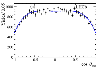
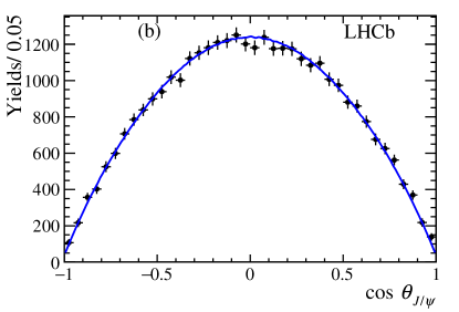
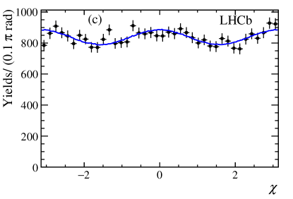
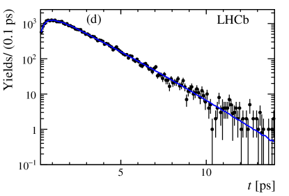
Figure 4: Projections of the angular and decay-time variables with the fit result overlaid. The points (black) show the data and the curves (blue) the fits.

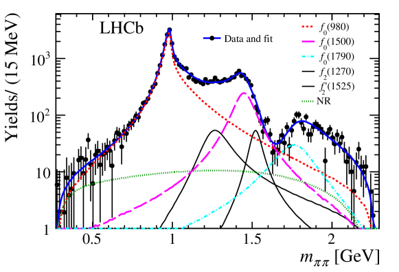
Figure 5: Data distribution of $m_{\pi\pi}$ with the projection of the Solution I fit result overlaid. The data are described by the points (black) with error bars. The solid (blue) curve shows the overall fit.

Table 5: Fit results of the resonant structure for both Solutions I and II. These results do not supersede those in Ref. [27] for the resonant fractions because no systematic uncertainties are quoted. The sum of fit fraction is not necessary 100% due to possible interferences between resonances with the same spin.

Component	Fit fractions (%)	Transversity fractions (%)
		$0$	$\parallel$	$\perp$
Solution I
$f_{0}(980)$	$\!\!\!60.09\pm 1.48$	$100$	$-$	$-$
$f_{0}(1500)$	$8.88\pm 0.87$	$100$	$-$	$-$
$f_{0}(1790)$	$1.72\pm 0.29$	$100$	$-$	$-$
$f_{2}(1270)$	$3.24\pm 0.48$	$\!\!\!13\pm 3$	$\!\!\!37\pm 9$	$50\pm 10$
$f_{2}^{\prime}(1525)$	$1.23\pm 0.86$	$40\pm 13$	$31\pm 14$	$29\pm 25$
NR	$2.64\pm 0.73$	$100$	$-$	$-$
Solution II
$f_{0}(980)$	$\!\!\!93.05\pm 1.12$	$100$	$-$	$-$
$f_{0}(1500)$	$6.47\pm 0.41$	$100$	$-$	$-$
$f_{0}(1710)$	$0.74\pm 0.11$	$100$	$-$	$-$
$f_{2}(1270)$	$3.22\pm 0.44$	$17\pm 4$	$\!\!\!30\pm 8$	$53\pm 10$
$f_{2}^{\prime}(1525)$	$1.44\pm 0.36$	$35\pm 8$	$31\pm 12$	$34\pm 17$
NR	$8.13\pm 0.79$	$100$	$-$	$-$

10 Systematic uncertainties

The systematic uncertainties for the $C\!P$-violating parameters, $\lambda$ and $\phi_{s}$, are smaller than the statistical ones. They are summarized in Table 6 along with the uncertainty on ${\Gamma_{\mathrm{H}}}-\Gamma_{{{B}^{0}}}$. The uncertainty on the decay-time acceptance is found by varying the parameters of the acceptance function within their uncertainties and repeating the fit. The same procedure is followed for the uncertainties on the ${B}^{0}$ lifetime, $\Delta m_{s}$, $\Gamma_{L}$, $m_{\pi\pi}$ and angular efficiencies, resonance masses and widths, flavour-tagging calibration, and allowing for a 2% production asymmetry [50]; this uncertainty also includes any possible difference in flavour tagging between ${\kern 1.79993pt\overline{\kern-1.79993ptB}}{}^{0}_{s}$ and ${B}^{0}_{s}$. Simulation is used to validate the method for the time-resolution calibration. The uncertainties of the parameters of the time-resolution model are estimated using the difference between the signal simulation and prompt ${{J\mskip-3.0mu/\mskip-2.0mu\psi\mskip 2.0mu}}$ simulation. These uncertainties are varied to obtain the effects on the physics parameters. Resonance modelling uncertainty includes varying the Breit–Wigner barrier factors, changing the default values of $L_{B}=1$ for the D-wave resonances to one or two, the differences between the two best solutions, and replacing the NR component by the $f_{0}(500)$ resonance. Furthermore, including an isospin-violating $\rho(770)^{0}$ component in the fit, results in a negligible contribution of $(1.1\pm 0.3)$%. The largest shift among the modelling variations is taken as systematic uncertainty. The inclusion of $\rho$ components results in the largest shifts of the three physics parameters quoted. The process $B_{c}^{+}\rightarrow\pi^{+}{{B}^{0}_{s}}$ can affect the measurement of ${\Gamma_{\mathrm{H}}}-\Gamma_{{{B}^{0}}}$. An estimate of the fraction of these decays in our sample is 0.8% [8]. Neglecting the ${{B}_{c}^{+}}$ contribution leads to a bias of 0.0005$\text{\,ps}^{-1}$, which is added as a systematic uncertainty. Other parameters are unchanged.

Corrections from penguin amplitudes are ignored because their effects are known to be small [51, 52, 53] compared to the current experimental precision.

Table 6: Absolute systematic uncertainties for the physics parameters.

Source	${\Gamma_{\mathrm{H}}}-\Gamma_{{{B}^{0}}}$	$|\lambda|$	${\phi_{{s}}}$
	[$\text{\,fs}^{-1}$]	$[\times 10^{-3}]$	[mrad]
Decay-time acceptance	$2.0$	$0.0$	$0.3$
$\tau_{{B}^{0}}$	$0.2$	$0.5$	$0.0$
Efficiency ($m_{\pi\pi}$, $\Omega$)	$0.2$	$0.1$	$0.0$
Decay-time resolution width	$0.0$	$4.3$	$4.0$
Decay-time resolution mean	$0.3$	$1.2$	$0.3$
Background	$3.0$	$2.7$	$0.6$
Flavour tagging	$0.0$	$2.2$	$2.3$
${\Delta m_{{s}}}$	$0.3$	$4.6$	$2.5$
${\Gamma_{\mathrm{L}}}$	$0.3$	$0.4$	$0.4$
${{B}_{c}^{+}}$	$0.5$	-	-
Resonance parameters	0.6	1.9	0.8
Resonance modelling	$0.5$	$28.9$	$9.0$
Production asymmetry	0.3	0.6	3.4
Total	$3.8$	$29.9$	$11.0$

11 Conclusions

Using ${{B}^{0}_{s}}$ and ${{\kern 1.79993pt\overline{\kern-1.79993ptB}}{}^{0}_{s}}\rightarrow{{J\mskip-3.0mu/\mskip-2.0mu\psi\mskip 2.0mu}}{{\pi}^{+}}{{\pi}^{-}}$ decays, we measure the $C\!P$-violating phase, ${\phi_{{s}}}=-0.057\pm 0.060\pm 0.011$ rad, the decay-width difference ${\Gamma_{\mathrm{H}}}-\Gamma_{{{B}^{0}}}=-0.050\pm 0.004\pm 0.004$ ​$\text{\,ps}^{-1}$, and the parameter $|\lambda|=1.01_{-0.06}^{+0.08}\pm 0.03$, where the quoted uncertainties are statistical and systematic. These results are more precise than those obtained from the previous study of this mode using 7 TeV and 8 TeV $pp$ collisions (Run 1) [7]. To combine the Run-1 results with these, we reanalyze them by fixing ${\Delta m_{{s}}}=17.757\pm 0.021$$\text{\,ps}^{-1}$ from Ref. [18], and ${\Gamma_{\mathrm{L}}}=0.6995\pm 0.0047$$\text{\,ps}^{-1}$ from the LHCb ${{B}^{0}_{s}}\rightarrow{{J\mskip-3.0mu/\mskip-2.0mu\psi\mskip 2.0mu}}K^{+}K^{-}$ results [9]. We remove the Gaussian constraint on ${\Delta\Gamma_{{s}}}$ and let ${\Gamma_{\mathrm{H}}}$ vary. Instead of taking the uncertainties of flavour tagging and decay-time resolution into the statistical uncertainty, we place these sources in the systematic uncertainty and assume 100% correlation with our new results. The updated results are: ${\phi_{{s}}}=0.075\pm 0.065\pm 0.014$ rad and $|\lambda|=0.898\pm 0.051\pm 0.013$ with a correlation of $0.025$. We then use the updated ${\phi_{{s}}}$ and $|\lambda|$ Run-1 results as a constraint into our new ${\phi_{{s}}}$ fit. The combined results are ${\Gamma_{\mathrm{H}}}-\Gamma_{{{B}^{0}}}=-0.050\pm 0.004\pm 0.004$ ​$\text{\,ps}^{-1}$, $|\lambda|=0.949\pm 0.036\pm 0.019$, and $\phi_{s}=0.002\pm 0.044\pm 0.012$ ​rad. The correlation coefficients among the fit parameters are 0.025 $(\rho_{12})$, –0.001 $(\rho_{13})$, and 0.026 $(\rho_{23})$.

Our results still have uncertainties greater than the SM prediction and are slightly more precise than the measurement using ${{B}^{0}_{s}}\rightarrow{{J\mskip-3.0mu/\mskip-2.0mu\psi\mskip 2.0mu}}K^{+}K^{-}$ decays, based only on Run-1 data, which has a precision of 0.049 rad [8]. Hence this is the most precise determination of $\phi_{s}$ to date.

LHCb Collaboration

R. Aaij²⁹, C. Abellán Beteta⁴⁶, B. Adeva⁴³, M. Adinolfi⁵⁰, C.A. Aidala⁷⁷, Z. Ajaltouni⁷, S. Akar⁶¹, P. Albicocco²⁰, J. Albrecht¹², F. Alessio⁴⁴, M. Alexander⁵⁵, A. Alfonso Albero⁴², G. Alkhazov⁴¹, P. Alvarez Cartelle⁵⁷, A.A. Alves Jr⁴³, S. Amato², Y. Amhis⁹, L. An¹⁹, L. Anderlini¹⁹, G. Andreassi⁴⁵, M. Andreotti¹⁸, J.E. Andrews⁶², F. Archilli²⁹, J. Arnau Romeu⁸, A. Artamonov⁴⁰, M. Artuso⁶³, K. Arzymatov³⁸, E. Aslanides⁸, M. Atzeni⁴⁶, B. Audurier²⁴, S. Bachmann¹⁴, J.J. Back⁵², S. Baker⁵⁷, V. Balagura^9,b, W. Baldini^18,44, A. Baranov³⁸, R.J. Barlow⁵⁸, G.C. Barrand⁹, S. Barsuk⁹, W. Barter⁵⁷, M. Bartolini²¹, F. Baryshnikov⁷³, V. Batozskaya³³, B. Batsukh⁶³, A. Battig¹², V. Battista⁴⁵, A. Bay⁴⁵, F. Bedeschi²⁶, I. Bediaga¹, A. Beiter⁶³, L.J. Bel²⁹, S. Belin²⁴, N. Beliy⁴, V. Bellee⁴⁵, N. Belloli^22,i, K. Belous⁴⁰, I. Belyaev³⁵, G. Bencivenni²⁰, E. Ben-Haim¹⁰, S. Benson²⁹, S. Beranek¹¹, A. Berezhnoy³⁶, R. Bernet⁴⁶, D. Berninghoff¹⁴, E. Bertholet¹⁰, A. Bertolin²⁵, C. Betancourt⁴⁶, F. Betti^17,e, M.O. Bettler⁵¹, Ia. Bezshyiko⁴⁶, S. Bhasin⁵⁰, J. Bhom³¹, M.S. Bieker¹², S. Bifani⁴⁹, P. Billoir¹⁰, A. Birnkraut¹², A. Bizzeti^19,u, M. Bjørn⁵⁹, M.P. Blago⁴⁴, T. Blake⁵², F. Blanc⁴⁵, S. Blusk⁶³, D. Bobulska⁵⁵, V. Bocci²⁸, O. Boente Garcia⁴³, T. Boettcher⁶⁰, A. Bondar^39,x, N. Bondar⁴¹, S. Borghi^58,44, M. Borisyak³⁸, M. Borsato¹⁴, M. Boubdir¹¹, T.J.V. Bowcock⁵⁶, C. Bozzi^18,44, S. Braun¹⁴, M. Brodski⁴⁴, J. Brodzicka³¹, A. Brossa Gonzalo⁵², D. Brundu^24,44, E. Buchanan⁵⁰, A. Buonaura⁴⁶, C. Burr⁵⁸, A. Bursche²⁴, J. Buytaert⁴⁴, W. Byczynski⁴⁴, S. Cadeddu²⁴, H. Cai⁶⁷, R. Calabrese^18,g, R. Calladine⁴⁹, M. Calvi^22,i, M. Calvo Gomez^42,m, A. Camboni^42,m, P. Campana²⁰, D.H. Campora Perez⁴⁴, L. Capriotti^17,e, A. Carbone^17,e, G. Carboni²⁷, R. Cardinale²¹, A. Cardini²⁴, P. Carniti^22,i, K. Carvalho Akiba², G. Casse⁵⁶, M. Cattaneo⁴⁴, G. Cavallero²¹, R. Cenci^26,p, D. Chamont⁹, M.G. Chapman⁵⁰, M. Charles^10,44, Ph. Charpentier⁴⁴, G. Chatzikonstantinidis⁴⁹, M. Chefdeville⁶, V. Chekalina³⁸, C. Chen³, S. Chen²⁴, S.-G. Chitic⁴⁴, V. Chobanova⁴³, M. Chrzaszcz⁴⁴, A. Chubykin⁴¹, P. Ciambrone²⁰, X. Cid Vidal⁴³, G. Ciezarek⁴⁴, F. Cindolo¹⁷, P.E.L. Clarke⁵⁴, M. Clemencic⁴⁴, H.V. Cliff⁵¹, J. Closier⁴⁴, V. Coco⁴⁴, J.A.B. Coelho⁹, J. Cogan⁸, E. Cogneras⁷, L. Cojocariu³⁴, P. Collins⁴⁴, T. Colombo⁴⁴, A. Comerma-Montells¹⁴, A. Contu²⁴, G. Coombs⁴⁴, S. Coquereau⁴², G. Corti⁴⁴, C.M. Costa Sobral⁵², B. Couturier⁴⁴, G.A. Cowan⁵⁴, D.C. Craik⁶⁰, A. Crocombe⁵², M. Cruz Torres¹, R. Currie⁵⁴, C.L. Da Silva⁷⁸, E. Dall’Occo²⁹, J. Dalseno^43,v, C. D’Ambrosio⁴⁴, A. Danilina³⁵, P. d’Argent¹⁴, A. Davis⁵⁸, O. De Aguiar Francisco⁴⁴, K. De Bruyn⁴⁴, S. De Capua⁵⁸, M. De Cian⁴⁵, J.M. De Miranda¹, L. De Paula², M. De Serio^16,d, P. De Simone²⁰, J.A. de Vries²⁹, C.T. Dean⁵⁵, W. Dean⁷⁷, D. Decamp⁶, L. Del Buono¹⁰, B. Delaney⁵¹, H.-P. Dembinski¹³, M. Demmer¹², A. Dendek³², D. Derkach⁷⁴, O. Deschamps⁷, F. Desse⁹, F. Dettori²⁴, B. Dey⁶⁸, A. Di Canto⁴⁴, P. Di Nezza²⁰, S. Didenko⁷³, H. Dijkstra⁴⁴, F. Dordei²⁴, M. Dorigo^44,y, A.C. dos Reis¹, A. Dosil Suárez⁴³, L. Douglas⁵⁵, A. Dovbnya⁴⁷, K. Dreimanis⁵⁶, L. Dufour⁴⁴, G. Dujany¹⁰, P. Durante⁴⁴, J.M. Durham⁷⁸, D. Dutta⁵⁸, R. Dzhelyadin^40,†, M. Dziewiecki¹⁴, A. Dziurda³¹, A. Dzyuba⁴¹, S. Easo⁵³, U. Egede⁵⁷, V. Egorychev³⁵, S. Eidelman^39,x, S. Eisenhardt⁵⁴, U. Eitschberger¹², R. Ekelhof¹², L. Eklund⁵⁵, S. Ely⁶³, A. Ene³⁴, S. Escher¹¹, S. Esen²⁹, T. Evans⁶¹, A. Falabella¹⁷, C. Färber⁴⁴, N. Farley⁴⁹, S. Farry⁵⁶, D. Fazzini^22,i, M. Féo⁴⁴, P. Fernandez Declara⁴⁴, A. Fernandez Prieto⁴³, F. Ferrari^17,e, L. Ferreira Lopes⁴⁵, F. Ferreira Rodrigues², S. Ferreres Sole²⁹, M. Ferro-Luzzi⁴⁴, S. Filippov³⁷, R.A. Fini¹⁶, M. Fiorini^18,g, M. Firlej³², C. Fitzpatrick⁴⁵, T. Fiutowski³², F. Fleuret^9,b, M. Fontana⁴⁴, F. Fontanelli^21,h, R. Forty⁴⁴, V. Franco Lima⁵⁶, M. Frank⁴⁴, C. Frei⁴⁴, J. Fu^23,q, W. Funk⁴⁴, E. Gabriel⁵⁴, A. Gallas Torreira⁴³, D. Galli^17,e, S. Gallorini²⁵, S. Gambetta⁵⁴, Y. Gan³, M. Gandelman², P. Gandini²³, Y. Gao³, L.M. Garcia Martin⁷⁶, J. García Pardiñas⁴⁶, B. Garcia Plana⁴³, J. Garra Tico⁵¹, L. Garrido⁴², D. Gascon⁴², C. Gaspar⁴⁴, G. Gazzoni⁷, D. Gerick¹⁴, E. Gersabeck⁵⁸, M. Gersabeck⁵⁸, T. Gershon⁵², D. Gerstel⁸, Ph. Ghez⁶, V. Gibson⁵¹, O.G. Girard⁴⁵, P. Gironella Gironell⁴², L. Giubega³⁴, K. Gizdov⁵⁴, V.V. Gligorov¹⁰, C. Göbel⁶⁵, D. Golubkov³⁵, A. Golutvin^57,73, A. Gomes^1,a, I.V. Gorelov³⁶, C. Gotti^22,i, E. Govorkova²⁹, J.P. Grabowski¹⁴, R. Graciani Diaz⁴², L.A. Granado Cardoso⁴⁴, E. Graugés⁴², E. Graverini⁴⁶, G. Graziani¹⁹, A. Grecu³⁴, R. Greim²⁹, P. Griffith²⁴, L. Grillo⁵⁸, L. Gruber⁴⁴, B.R. Gruberg Cazon⁵⁹, C. Gu³, E. Gushchin³⁷, A. Guth¹¹, Yu. Guz^40,44, T. Gys⁴⁴, T. Hadavizadeh⁵⁹, C. Hadjivasiliou⁷, G. Haefeli⁴⁵, C. Haen⁴⁴, S.C. Haines⁵¹, B. Hamilton⁶², X. Han¹⁴, T.H. Hancock⁵⁹, S. Hansmann-Menzemer¹⁴, N. Harnew⁵⁹, T. Harrison⁵⁶, C. Hasse⁴⁴, M. Hatch⁴⁴, J. He⁴, M. Hecker⁵⁷, K. Heinicke¹², A. Heister¹², K. Hennessy⁵⁶, L. Henry⁷⁶, M. Heß⁷⁰, J. Heuel¹¹, A. Hicheur⁶⁴, R. Hidalgo Charman⁵⁸, D. Hill⁵⁹, M. Hilton⁵⁸, P.H. Hopchev⁴⁵, J. Hu¹⁴, W. Hu⁶⁸, W. Huang⁴, Z.C. Huard⁶¹, W. Hulsbergen²⁹, T. Humair⁵⁷, M. Hushchyn⁷⁴, D. Hutchcroft⁵⁶, D. Hynds²⁹, P. Ibis¹², M. Idzik³², P. Ilten⁴⁹, A. Inglessi⁴¹, A. Inyakin⁴⁰, K. Ivshin⁴¹, R. Jacobsson⁴⁴, S. Jakobsen⁴⁴, J. Jalocha⁵⁹, E. Jans²⁹, B.K. Jashal⁷⁶, A. Jawahery⁶², F. Jiang³, M. John⁵⁹, D. Johnson⁴⁴, C.R. Jones⁵¹, C. Joram⁴⁴, B. Jost⁴⁴, N. Jurik⁵⁹, S. Kandybei⁴⁷, M. Karacson⁴⁴, J.M. Kariuki⁵⁰, S. Karodia⁵⁵, N. Kazeev⁷⁴, M. Kecke¹⁴, F. Keizer⁵¹, M. Kelsey⁶³, M. Kenzie⁵¹, T. Ketel³⁰, B. Khanji⁴⁴, A. Kharisova⁷⁵, C. Khurewathanakul⁴⁵, K.E. Kim⁶³, T. Kirn¹¹, V.S. Kirsebom⁴⁵, S. Klaver²⁰, K. Klimaszewski³³, S. Koliiev⁴⁸, M. Kolpin¹⁴, R. Kopecna¹⁴, P. Koppenburg²⁹, I. Kostiuk^29,48, S. Kotriakhova⁴¹, M. Kozeiha⁷, L. Kravchuk³⁷, M. Kreps⁵², F. Kress⁵⁷, S. Kretzschmar¹¹, P. Krokovny^39,x, W. Krupa³², W. Krzemien³³, W. Kucewicz^31,l, M. Kucharczyk³¹, V. Kudryavtsev^39,x, G.J. Kunde⁷⁸, A.K. Kuonen⁴⁵, T. Kvaratskheliya³⁵, D. Lacarrere⁴⁴, G. Lafferty⁵⁸, A. Lai²⁴, D. Lancierini⁴⁶, G. Lanfranchi²⁰, C. Langenbruch¹¹, T. Latham⁵², C. Lazzeroni⁴⁹, R. Le Gac⁸, R. Lefèvre⁷, A. Leflat³⁶, F. Lemaitre⁴⁴, O. Leroy⁸, T. Lesiak³¹, B. Leverington¹⁴, H. Li⁶⁶, P.-R. Li^4,ab, Y. Li⁵, Z. Li⁶³, X. Liang⁶³, T. Likhomanenko⁷², R. Lindner⁴⁴, F. Lionetto⁴⁶, V. Lisovskyi⁹, G. Liu⁶⁶, X. Liu³, D. Loh⁵², A. Loi²⁴, I. Longstaff⁵⁵, J.H. Lopes², G. Loustau⁴⁶, G.H. Lovell⁵¹, D. Lucchesi^25,o, M. Lucio Martinez⁴³, Y. Luo³, A. Lupato²⁵, E. Luppi^18,g, O. Lupton⁵², A. Lusiani²⁶, X. Lyu⁴, F. Machefert⁹, F. Maciuc³⁴, V. Macko⁴⁵, P. Mackowiak¹², S. Maddrell-Mander⁵⁰, O. Maev^41,44, K. Maguire⁵⁸, D. Maisuzenko⁴¹, M.W. Majewski³², S. Malde⁵⁹, B. Malecki⁴⁴, A. Malinin⁷², T. Maltsev^39,x, H. Malygina¹⁴, G. Manca^24,f, G. Mancinelli⁸, D. Marangotto^23,q, J. Maratas^7,w, J.F. Marchand⁶, U. Marconi¹⁷, C. Marin Benito⁹, M. Marinangeli⁴⁵, P. Marino⁴⁵, J. Marks¹⁴, P.J. Marshall⁵⁶, G. Martellotti²⁸, M. Martinelli^44,22, D. Martinez Santos⁴³, F. Martinez Vidal⁷⁶, A. Massafferri¹, M. Materok¹¹, R. Matev⁴⁴, A. Mathad⁴⁶, Z. Mathe⁴⁴, V. Matiunin³⁵, C. Matteuzzi²², K.R. Mattioli⁷⁷, A. Mauri⁴⁶, E. Maurice^9,b, B. Maurin⁴⁵, M. McCann^57,44, A. McNab⁵⁸, R. McNulty¹⁵, J.V. Mead⁵⁶, B. Meadows⁶¹, C. Meaux⁸, N. Meinert⁷⁰, D. Melnychuk³³, M. Merk²⁹, A. Merli^23,q, E. Michielin²⁵, D.A. Milanes⁶⁹, E. Millard⁵², M.-N. Minard⁶, L. Minzoni^18,g, D.S. Mitzel¹⁴, A. Mödden¹², A. Mogini¹⁰, R.D. Moise⁵⁷, T. Mombächer¹², I.A. Monroy⁶⁹, S. Monteil⁷, M. Morandin²⁵, G. Morello²⁰, M.J. Morello^26,t, J. Moron³², A.B. Morris⁸, R. Mountain⁶³, F. Muheim⁵⁴, M. Mukherjee⁶⁸, M. Mulder²⁹, D. Müller⁴⁴, J. Müller¹², K. Müller⁴⁶, V. Müller¹², C.H. Murphy⁵⁹, D. Murray⁵⁸, P. Naik⁵⁰, T. Nakada⁴⁵, R. Nandakumar⁵³, A. Nandi⁵⁹, T. Nanut⁴⁵, I. Nasteva², M. Needham⁵⁴, N. Neri^23,q, S. Neubert¹⁴, N. Neufeld⁴⁴, R. Newcombe⁵⁷, T.D. Nguyen⁴⁵, C. Nguyen-Mau^45,n, S. Nieswand¹¹, R. Niet¹², N. Nikitin³⁶, N.S. Nolte⁴⁴, A. Oblakowska-Mucha³², V. Obraztsov⁴⁰, S. Ogilvy⁵⁵, D.P. O’Hanlon¹⁷, R. Oldeman^24,f, C.J.G. Onderwater⁷¹, J. D. Osborn⁷⁷, A. Ossowska³¹, J.M. Otalora Goicochea², T. Ovsiannikova³⁵, P. Owen⁴⁶, A. Oyanguren⁷⁶, P.R. Pais⁴⁵, T. Pajero^26,t, A. Palano¹⁶, M. Palutan²⁰, G. Panshin⁷⁵, A. Papanestis⁵³, M. Pappagallo⁵⁴, L.L. Pappalardo^18,g, W. Parker⁶², C. Parkes^58,44, G. Passaleva^19,44, A. Pastore¹⁶, M. Patel⁵⁷, C. Patrignani^17,e, A. Pearce⁴⁴, A. Pellegrino²⁹, G. Penso²⁸, M. Pepe Altarelli⁴⁴, S. Perazzini⁴⁴, D. Pereima³⁵, P. Perret⁷, L. Pescatore⁴⁵, K. Petridis⁵⁰, A. Petrolini^21,h, A. Petrov⁷², S. Petrucci⁵⁴, M. Petruzzo^23,q, B. Pietrzyk⁶, G. Pietrzyk⁴⁵, M. Pikies³¹, M. Pili⁵⁹, D. Pinci²⁸, J. Pinzino⁴⁴, F. Pisani⁴⁴, A. Piucci¹⁴, V. Placinta³⁴, S. Playfer⁵⁴, J. Plews⁴⁹, M. Plo Casasus⁴³, F. Polci¹⁰, M. Poli Lener²⁰, M. Poliakova⁶³, A. Poluektov⁸, N. Polukhina^73,c, I. Polyakov⁶³, E. Polycarpo², G.J. Pomery⁵⁰, S. Ponce⁴⁴, A. Popov⁴⁰, D. Popov^49,13, S. Poslavskii⁴⁰, E. Price⁵⁰, C. Prouve⁴³, V. Pugatch⁴⁸, A. Puig Navarro⁴⁶, H. Pullen⁵⁹, G. Punzi^26,p, W. Qian⁴, J. Qin⁴, R. Quagliani¹⁰, B. Quintana⁷, N.V. Raab¹⁵, B. Rachwal³², J.H. Rademacker⁵⁰, M. Rama²⁶, M. Ramos Pernas⁴³, M.S. Rangel², F. Ratnikov^38,74, G. Raven³⁰, M. Ravonel Salzgeber⁴⁴, M. Reboud⁶, F. Redi⁴⁵, S. Reichert¹², F. Reiss¹⁰, C. Remon Alepuz⁷⁶, Z. Ren³, V. Renaudin⁵⁹, S. Ricciardi⁵³, S. Richards⁵⁰, K. Rinnert⁵⁶, P. Robbe⁹, A. Robert¹⁰, A.B. Rodrigues⁴⁵, E. Rodrigues⁶¹, J.A. Rodriguez Lopez⁶⁹, M. Roehrken⁴⁴, S. Roiser⁴⁴, A. Rollings⁵⁹, V. Romanovskiy⁴⁰, A. Romero Vidal⁴³, J.D. Roth⁷⁷, M. Rotondo²⁰, M.S. Rudolph⁶³, T. Ruf⁴⁴, J. Ruiz Vidal⁷⁶, J.J. Saborido Silva⁴³, N. Sagidova⁴¹, B. Saitta^24,f, V. Salustino Guimaraes⁶⁵, C. Sanchez Gras²⁹, C. Sanchez Mayordomo⁷⁶, B. Sanmartin Sedes⁴³, R. Santacesaria²⁸, C. Santamarina Rios⁴³, M. Santimaria^20,44, E. Santovetti^27,j, G. Sarpis⁵⁸, A. Sarti^20,k, C. Satriano^28,s, A. Satta²⁷, M. Saur⁴, D. Savrina^35,36, S. Schael¹¹, M. Schellenberg¹², M. Schiller⁵⁵, H. Schindler⁴⁴, M. Schmelling¹³, T. Schmelzer¹², B. Schmidt⁴⁴, O. Schneider⁴⁵, A. Schopper⁴⁴, H.F. Schreiner⁶¹, M. Schubiger⁴⁵, S. Schulte⁴⁵, M.H. Schune⁹, R. Schwemmer⁴⁴, B. Sciascia²⁰, A. Sciubba^28,k, A. Semennikov³⁵, E.S. Sepulveda¹⁰, A. Sergi^49,44, N. Serra⁴⁶, J. Serrano⁸, L. Sestini²⁵, A. Seuthe¹², P. Seyfert⁴⁴, M. Shapkin⁴⁰, T. Shears⁵⁶, L. Shekhtman^39,x, V. Shevchenko⁷², E. Shmanin⁷³, B.G. Siddi¹⁸, R. Silva Coutinho⁴⁶, L. Silva de Oliveira², G. Simi^25,o, S. Simone^16,d, I. Skiba¹⁸, N. Skidmore¹⁴, T. Skwarnicki⁶³, M.W. Slater⁴⁹, J.G. Smeaton⁵¹, E. Smith¹¹, I.T. Smith⁵⁴, M. Smith⁵⁷, M. Soares¹⁷, l. Soares Lavra¹, M.D. Sokoloff⁶¹, F.J.P. Soler⁵⁵, B. Souza De Paula², B. Spaan¹², E. Spadaro Norella^23,q, P. Spradlin⁵⁵, F. Stagni⁴⁴, M. Stahl¹⁴, S. Stahl⁴⁴, P. Stefko⁴⁵, S. Stefkova⁵⁷, O. Steinkamp⁴⁶, S. Stemmle¹⁴, O. Stenyakin⁴⁰, M. Stepanova⁴¹, H. Stevens¹², A. Stocchi⁹, S. Stone⁶³, S. Stracka²⁶, M.E. Stramaglia⁴⁵, M. Straticiuc³⁴, U. Straumann⁴⁶, S. Strokov⁷⁵, J. Sun³, L. Sun⁶⁷, Y. Sun⁶², K. Swientek³², A. Szabelski³³, T. Szumlak³², M. Szymanski⁴, Z. Tang³, T. Tekampe¹², G. Tellarini¹⁸, F. Teubert⁴⁴, E. Thomas⁴⁴, M.J. Tilley⁵⁷, V. Tisserand⁷, S. T’Jampens⁶, M. Tobin⁵, S. Tolk⁴⁴, L. Tomassetti^18,g, D. Tonelli²⁶, D.Y. Tou¹⁰, R. Tourinho Jadallah Aoude¹, E. Tournefier⁶, M. Traill⁵⁵, M.T. Tran⁴⁵, A. Trisovic⁵¹, A. Tsaregorodtsev⁸, G. Tuci^26,44,p, A. Tully⁵¹, N. Tuning²⁹, A. Ukleja³³, A. Usachov⁹, A. Ustyuzhanin^38,74, U. Uwer¹⁴, A. Vagner⁷⁵, V. Vagnoni¹⁷, A. Valassi⁴⁴, S. Valat⁴⁴, G. Valenti¹⁷, M. van Beuzekom²⁹, H. Van Hecke⁷⁸, E. van Herwijnen⁴⁴, C.B. Van Hulse¹⁵, J. van Tilburg²⁹, M. van Veghel²⁹, R. Vazquez Gomez⁴⁴, P. Vazquez Regueiro⁴³, C. Vázquez Sierra²⁹, S. Vecchi¹⁸, J.J. Velthuis⁵⁰, M. Veltri^19,r, A. Venkateswaran⁶³, M. Vernet⁷, M. Veronesi²⁹, M. Vesterinen⁵², J.V. Viana Barbosa⁴⁴, D. Vieira⁴, M. Vieites Diaz⁴³, H. Viemann⁷⁰, X. Vilasis-Cardona^42,m, A. Vitkovskiy²⁹, M. Vitti⁵¹, V. Volkov³⁶, A. Vollhardt⁴⁶, D. Vom Bruch¹⁰, B. Voneki⁴⁴, A. Vorobyev⁴¹, V. Vorobyev^39,x, N. Voropaev⁴¹, R. Waldi⁷⁰, J. Walsh²⁶, J. Wang⁵, M. Wang³, Y. Wang⁶⁸, Z. Wang⁴⁶, D.R. Ward⁵¹, H.M. Wark⁵⁶, N.K. Watson⁴⁹, D. Websdale⁵⁷, A. Weiden⁴⁶, C. Weisser⁶⁰, M. Whitehead¹¹, G. Wilkinson⁵⁹, M. Wilkinson⁶³, I. Williams⁵¹, M. Williams⁶⁰, M.R.J. Williams⁵⁸, T. Williams⁴⁹, F.F. Wilson⁵³, M. Winn⁹, W. Wislicki³³, M. Witek³¹, G. Wormser⁹, S.A. Wotton⁵¹, K. Wyllie⁴⁴, D. Xiao⁶⁸, Y. Xie⁶⁸, H. Xing⁶⁶, A. Xu³, M. Xu⁶⁸, Q. Xu⁴, Z. Xu⁶, Z. Xu³, Z. Yang³, Z. Yang⁶², Y. Yao⁶³, L.E. Yeomans⁵⁶, H. Yin⁶⁸, J. Yu^68,aa, X. Yuan⁶³, O. Yushchenko⁴⁰, K.A. Zarebski⁴⁹, M. Zavertyaev^13,c, M. Zeng³, D. Zhang⁶⁸, L. Zhang³, W.C. Zhang^3,z, Y. Zhang⁴⁴, A. Zhelezov¹⁴, Y. Zheng⁴, X. Zhu³, V. Zhukov^11,36, J.B. Zonneveld⁵⁴, S. Zucchelli^17,e.

¹Centro Brasileiro de Pesquisas Físicas (CBPF), Rio de Janeiro, Brazil
²Universidade Federal do Rio de Janeiro (UFRJ), Rio de Janeiro, Brazil
³Center for High Energy Physics, Tsinghua University, Beijing, China
⁴University of Chinese Academy of Sciences, Beijing, China
⁵Institute Of High Energy Physics (ihep), Beijing, China
⁶Univ. Grenoble Alpes, Univ. Savoie Mont Blanc, CNRS, IN2P3-LAPP, Annecy, France
⁷Université Clermont Auvergne, CNRS/IN2P3, LPC, Clermont-Ferrand, France
⁸Aix Marseille Univ, CNRS/IN2P3, CPPM, Marseille, France
⁹LAL, Univ. Paris-Sud, CNRS/IN2P3, Université Paris-Saclay, Orsay, France
¹⁰LPNHE, Sorbonne Université, Paris Diderot Sorbonne Paris Cité, CNRS/IN2P3, Paris, France
¹¹I. Physikalisches Institut, RWTH Aachen University, Aachen, Germany
¹²Fakultät Physik, Technische Universität Dortmund, Dortmund, Germany
¹³Max-Planck-Institut für Kernphysik (MPIK), Heidelberg, Germany
¹⁴Physikalisches Institut, Ruprecht-Karls-Universität Heidelberg, Heidelberg, Germany
¹⁵School of Physics, University College Dublin, Dublin, Ireland
¹⁶INFN Sezione di Bari, Bari, Italy
¹⁷INFN Sezione di Bologna, Bologna, Italy
¹⁸INFN Sezione di Ferrara, Ferrara, Italy
¹⁹INFN Sezione di Firenze, Firenze, Italy
²⁰INFN Laboratori Nazionali di Frascati, Frascati, Italy
²¹INFN Sezione di Genova, Genova, Italy
²²INFN Sezione di Milano-Bicocca, Milano, Italy
²³INFN Sezione di Milano, Milano, Italy
²⁴INFN Sezione di Cagliari, Monserrato, Italy
²⁵INFN Sezione di Padova, Padova, Italy
²⁶INFN Sezione di Pisa, Pisa, Italy
²⁷INFN Sezione di Roma Tor Vergata, Roma, Italy
²⁸INFN Sezione di Roma La Sapienza, Roma, Italy
²⁹Nikhef National Institute for Subatomic Physics, Amsterdam, Netherlands
³⁰Nikhef National Institute for Subatomic Physics and VU University Amsterdam, Amsterdam, Netherlands
³¹Henryk Niewodniczanski Institute of Nuclear Physics Polish Academy of Sciences, Kraków, Poland
³²AGH - University of Science and Technology, Faculty of Physics and Applied Computer Science, Kraków, Poland
³³National Center for Nuclear Research (NCBJ), Warsaw, Poland
³⁴Horia Hulubei National Institute of Physics and Nuclear Engineering, Bucharest-Magurele, Romania
³⁵Institute of Theoretical and Experimental Physics NRC Kurchatov Institute (ITEP NRC KI), Moscow, Russia, Moscow, Russia
³⁶Institute of Nuclear Physics, Moscow State University (SINP MSU), Moscow, Russia
³⁷Institute for Nuclear Research of the Russian Academy of Sciences (INR RAS), Moscow, Russia
³⁸Yandex School of Data Analysis, Moscow, Russia
³⁹Budker Institute of Nuclear Physics (SB RAS), Novosibirsk, Russia
⁴⁰Institute for High Energy Physics NRC Kurchatov Institute (IHEP NRC KI), Protvino, Russia, Protvino, Russia
⁴¹Petersburg Nuclear Physics Institute NRC Kurchatov Institute (PNPI NRC KI), Gatchina, Russia , St.Petersburg, Russia
⁴²ICCUB, Universitat de Barcelona, Barcelona, Spain
⁴³Instituto Galego de Física de Altas Enerxías (IGFAE), Universidade de Santiago de Compostela, Santiago de Compostela, Spain
⁴⁴European Organization for Nuclear Research (CERN), Geneva, Switzerland
⁴⁵Institute of Physics, Ecole Polytechnique Fédérale de Lausanne (EPFL), Lausanne, Switzerland
⁴⁶Physik-Institut, Universität Zürich, Zürich, Switzerland
⁴⁷NSC Kharkiv Institute of Physics and Technology (NSC KIPT), Kharkiv, Ukraine
⁴⁸Institute for Nuclear Research of the National Academy of Sciences (KINR), Kyiv, Ukraine
⁴⁹University of Birmingham, Birmingham, United Kingdom
⁵⁰H.H. Wills Physics Laboratory, University of Bristol, Bristol, United Kingdom
⁵¹Cavendish Laboratory, University of Cambridge, Cambridge, United Kingdom
⁵²Department of Physics, University of Warwick, Coventry, United Kingdom
⁵³STFC Rutherford Appleton Laboratory, Didcot, United Kingdom
⁵⁴School of Physics and Astronomy, University of Edinburgh, Edinburgh, United Kingdom
⁵⁵School of Physics and Astronomy, University of Glasgow, Glasgow, United Kingdom
⁵⁶Oliver Lodge Laboratory, University of Liverpool, Liverpool, United Kingdom
⁵⁷Imperial College London, London, United Kingdom
⁵⁸School of Physics and Astronomy, University of Manchester, Manchester, United Kingdom
⁵⁹Department of Physics, University of Oxford, Oxford, United Kingdom
⁶⁰Massachusetts Institute of Technology, Cambridge, MA, United States
⁶¹University of Cincinnati, Cincinnati, OH, United States
⁶²University of Maryland, College Park, MD, United States
⁶³Syracuse University, Syracuse, NY, United States
⁶⁴Laboratory of Mathematical and Subatomic Physics , Constantine, Algeria, associated to ^2
65Pontifícia Universidade Católica do Rio de Janeiro (PUC-Rio), Rio de Janeiro, Brazil, associated to ^2
66South China Normal University, Guangzhou, China, associated to ^3
67School of Physics and Technology, Wuhan University, Wuhan, China, associated to ^3
68Institute of Particle Physics, Central China Normal University, Wuhan, Hubei, China, associated to ^3
69Departamento de Fisica , Universidad Nacional de Colombia, Bogota, Colombia, associated to ^10
70Institut für Physik, Universität Rostock, Rostock, Germany, associated to ^14
71Van Swinderen Institute, University of Groningen, Groningen, Netherlands, associated to ^29
72National Research Centre Kurchatov Institute, Moscow, Russia, associated to ^35
73National University of Science and Technology “MISIS”, Moscow, Russia, associated to ^35
74National Research University Higher School of Economics, Moscow, Russia, associated to ^38
75National Research Tomsk Polytechnic University, Tomsk, Russia, associated to ^35
76Instituto de Fisica Corpuscular, Centro Mixto Universidad de Valencia - CSIC, Valencia, Spain, associated to ^42
77University of Michigan, Ann Arbor, United States, associated to ^63
78Los Alamos National Laboratory (LANL), Los Alamos, United States, associated to <sup>63

a</sup>Universidade Federal do Triângulo Mineiro (UFTM), Uberaba-MG, Brazil
^bLaboratoire Leprince-Ringuet, Palaiseau, France
^cP.N. Lebedev Physical Institute, Russian Academy of Science (LPI RAS), Moscow, Russia
^dUniversità di Bari, Bari, Italy
^eUniversità di Bologna, Bologna, Italy
^fUniversità di Cagliari, Cagliari, Italy
^gUniversità di Ferrara, Ferrara, Italy
^hUniversità di Genova, Genova, Italy
ⁱUniversità di Milano Bicocca, Milano, Italy
^jUniversità di Roma Tor Vergata, Roma, Italy
^kUniversità di Roma La Sapienza, Roma, Italy
^lAGH - University of Science and Technology, Faculty of Computer Science, Electronics and Telecommunications, Kraków, Poland
^mLIFAELS, La Salle, Universitat Ramon Llull, Barcelona, Spain
ⁿHanoi University of Science, Hanoi, Vietnam
^oUniversità di Padova, Padova, Italy
^pUniversità di Pisa, Pisa, Italy
^qUniversità degli Studi di Milano, Milano, Italy
^rUniversità di Urbino, Urbino, Italy
^sUniversità della Basilicata, Potenza, Italy
^tScuola Normale Superiore, Pisa, Italy
^uUniversità di Modena e Reggio Emilia, Modena, Italy
^vH.H. Wills Physics Laboratory, University of Bristol, Bristol, United Kingdom
^wMSU - Iligan Institute of Technology (MSU-IIT), Iligan, Philippines
^xNovosibirsk State University, Novosibirsk, Russia
^ySezione INFN di Trieste, Trieste, Italy
^zSchool of Physics and Information Technology, Shaanxi Normal University (SNNU), Xi’an, China
^aaPhysics and Micro Electronic College, Hunan University, Changsha City, China
^abLanzhou University, Lanzhou, China
^†Deceased

References

- [1] I. I. Y. Bigi and A. I. Sanda, CP violation, Camb. Monogr. Part. Phys. Nucl. Phys. Cosmol. 9 (2000) 1
- [2] CKMfitter group, J. Charles et al., Current status of the Standard Model CKM fit and constraints on new physics, Phys. Rev. D91 (2015) 073007, arXiv:1501.05013, updated results and plots available at http://ckmfitter.in2p3.fr/
- [3] CDF collaboration, T. Aaltonen et al., First flavor-tagged determination of bounds on mixing-induced CP violation in decays, Phys. Rev. Lett. 100 (2008) 161802, arXiv:0712.2397
- [4] D0 collaboration, V. M. Abazov et al., Measurement of mixing parameters from the flavor-tagged decay , Phys. Rev. Lett. 101 (2008) 241801, arXiv:0802.2255
- [5] CDF collaboration, T. Aaltonen et al., Measurement of the -violating phase in decays with the CDF II detector, Phys. Rev. D85 (2012) 072002, arXiv:1112.1726
- [6] D0 collaboration, V. M. Abazov et al., Measurement of the -violating phase using the flavor-tagged decay in 8 fb-1 of collisions, Phys. Rev. D85 (2012) 032006, arXiv:1109.3166
- [7] LHCb collaboration, R. Aaij et al., Measurement of the -violating phase in decays, Phys. Lett. B736 (2014) 186, arXiv:1405.4140
- [8] LHCb collaboration, R. Aaij et al., Precision measurement of violation in decays, Phys. Rev. Lett. 114 (2015) 041801, arXiv:1411.3104
- [9] LHCb collaboration, R. Aaij et al., Resonances and violation in and decays in the mass region above the , JHEP 08 (2017) 037, arXiv:1704.08217
- [10] ATLAS collaboration, G. Aad et al., Measurement of the -violating phase and the meson decay width difference with decays in ATLAS, JHEP 08 (2016) 147, arXiv:1601.03297
- [11] CMS collaboration, V. Khachatryan et al., Measurement of the -violating weak phase and the decay width difference using the decay channel in pp collisions at 8 TeV, Phys. Lett. B757 (2016) 97, arXiv:1507.07527
- [12] S. Stone and L. Zhang, S-waves and the measurement of CP violating phases in decays, Phys. Rev. D79 (2009) 074024, arXiv:0812.2832
- [13] LHCb collaboration, A. A. Alves Jr. et al., The LHCb detector at the LHC, JINST 3 (2008) S08005
- [14] LHCb collaboration, R. Aaij et al., LHCb detector performance, Int. J. Mod. Phys. A30 (2015) 1530022, arXiv:1412.6352
- [15] R. Aaij et al., Performance of the LHCb Vertex Locator, JINST 9 (2014) P09007, arXiv:1405.7808
- [16] M. Adinolfi et al., Performance of the LHCb RICH detector at the LHC, Eur. Phys. J. C73 (2013) 2431, arXiv:1211.6759
- [17] A. A. Alves Jr. et al., Performance of the LHCb muon system, JINST 8 (2013) P02022, arXiv:1211.1346
- [18] Particle Data Group, M. Tanabashi et al., Review of particle physics, Phys. Rev. D98 (2018) 030001
- [19] T. Sjöstrand, S. Mrenna, and P. Skands, PYTHIA 6.4 physics and manual, JHEP 05 (2006) 026, arXiv:hep-ph/0603175
- [20] T. Sjöstrand, S. Mrenna, and P. Skands, A brief introduction to PYTHIA 8.1, Comput. Phys. Commun. 178 (2008) 852, arXiv:0710.3820
- [21] I. Belyaev et al., Handling of the generation of primary events in Gauss, the LHCb simulation framework, J. Phys. Conf. Ser. 331 (2011) 032047
- [22] D. J. Lange, The EvtGen particle decay simulation package, Nucl. Instrum. Meth. A462 (2001) 152
- [23] P. Golonka and Z. Was, PHOTOS Monte Carlo: A precision tool for QED corrections in and decays, Eur. Phys. J. C45 (2006) 97, arXiv:hep-ph/0506026
- [24] Geant4 collaboration, J. Allison et al., Geant4 developments and applications, IEEE Trans. Nucl. Sci. 53 (2006) 270
- [25] Geant4 collaboration, S. Agostinelli et al., Geant4: A simulation toolkit, Nucl. Instrum. Meth. A506 (2003) 250
- [26] M. Clemencic et al., The LHCb simulation application, Gauss: Design, evolution and experience, J. Phys. Conf. Ser. 331 (2011) 032023
- [27] LHCb collaboration, R. Aaij et al., Measurement of resonant and components in decays, Phys. Rev. D89 (2014) 092006, arXiv:1402.6248
- [28] L. Zhang and S. Stone, Time-dependent Dalitz-plot formalism for , Phys. Lett. B719 (2013) 383, arXiv:1212.6434
- [29] A. S. Dighe, I. Dunietz, H. J. Lipkin, and J. L. Rosner, Angular distributions and lifetime differences in decays, Phys. Lett. B369 (1996) 144, arXiv:hep-ph/9511363
- [30] LHCb collaboration, R. Aaij et al., Measurement of violation and the meson decay width difference with and decays, Phys. Rev. D87 (2013) 112010, arXiv:1304.2600
- [31] LHCb collaboration, R. Aaij et al., Measurement of the asymmetry in – mixing, Phys. Rev. Lett. 117 (2016) 061803, arXiv:1605.09768
- [32] U. Nierste, Three lectures on meson mixing and CKM phenomenology, arXiv:0904.1869
- [33] LHCb collaboration, R. Aaij et al., Opposite-side flavour tagging of B mesons at the LHCb experiment, Eur. Phys. J. C72 (2012) 2022, arXiv:1202.4979
- [34] LHCb collaboration, R. Aaij et al., A new algorithm for identifying the flavour of mesons at LHCb, JINST 11 (2016) P05010, arXiv:1602.07252
- [35] D. Fazzini, Flavour Tagging in the LHCb experiment, PoS LHCP2018 (2018) 230
- [36] L. Breiman, J. H. Friedman, R. A. Olshen, and C. J. Stone, Classification and regression trees, Wadsworth international group, Belmont, California, USA, 1984
- [37] Y. Freund and R. E. Schapire, A decision-theoretic generalization of on-line learning and an application to boosting, J. Comput. Syst. Sci. 55 (1997) 119
- [38] J. Stevens and M. Williams, uBoost: A boosting method for producing uniform selection efficiencies from multivariate classifiers, JINST 8 (2013) P12013, arXiv:1305.7248
- [39] W. D. Hulsbergen, Decay chain fitting with a Kalman filter, Nucl. Instrum. Meth. A552 (2005) 566, arXiv:physics/0503191
- [40] D. Martínez Santos and F. Dupertuis, Mass distributions marginalized over per-event errors, Nucl. Instrum. Meth. A764 (2014) 150, arXiv:1312.5000
- [41] LHCb collaboration, R. Aaij et al., Observation of the decay , Phys. Lett. B747 (2015) 484, arXiv:1503.07112
- [42] S. M. Flatté, On the nature of mesons, Phys. Lett. B63 (1976) 228
- [43] J. Daub, C. Hanhart, and B. Kubis, A model-independent analysis of final-state interactions in , JHEP 02 (2016) 009, arXiv:1508.06841
- [44] S. Ropertz, C. Hanhart, and B. Kubis, A new parametrization for the scalar pion form factors, Eur. Phys. J. C78 (2018) 1000, arXiv:1809.06867
- [45] BES collaboration, M. Ablikim et al., Resonances in and , Phys. Lett. B607 (2005) 243, arXiv:hep-ex/0411001
- [46] LHCb collaboration, R. Aaij et al., Analysis of the resonant components in , Phys. Rev. D87 (2013) 052001, arXiv:1301.5347
- [47] LHCb collaboration, R. Aaij et al., Analysis of the resonant components in , Phys. Rev. D86 (2012) 052006, arXiv:1204.5643
- [48] M. Pivk and F. R. Le Diberder, sPlot: A statistical tool to unfold data distributions, Nucl. Instrum. Meth. A555 (2005) 356, arXiv:physics/0402083
- [49] Y. Xie, sFit: a method for background subtraction in maximum likelihood fit, arXiv:0905.0724
- [50] LHCb collaboration, R. Aaij et al., Measurement of , , and production asymmetries in and TeV proton-proton collisions, Phys. Lett. B774 (2017) 139, arXiv:1703.08464
- [51] R. Fleischer, Theoretical prospects for B physics, PoS FPCP2015 (2015) 002, arXiv:1509.00601
- [52] LHCb collaboration, R. Aaij et al., Measurement of the -violating phase in decays and limits on penguin effects, Phys. Lett. B742 (2015) 38, arXiv:1411.1634
- [53] LHCb collaboration, R. Aaij et al., Measurement of violation parameters and polarisation fractions in decays, JHEP 11 (2015) 082, arXiv:1509.00400