On Inversely Proportional Hypermutations with Mutation Potential

Abstract.

Artificial Immune Systems (AIS) employing hypermutations with linear static mutation potential have recently been shown to be very effective at escaping local optima of combinatorial optimisation problems at the expense of being slower during the exploitation phase compared to standard evolutionary algorithms. In this paper we prove that considerable speed-ups in the exploitation phase may be achieved with dynamic inversely proportional mutation potentials (IPM) and argue that the potential should decrease inversely to the distance to the optimum rather than to the difference in fitness. Afterwards we define a simple (1+1) Opt-IA, that uses IPM hypermutations and ageing, for realistic applications where optimal solutions are unknown. The aim of the AIS is to approximate the ideal behaviour of the inversely proportional hypermutations better and better as the search space is explored. We prove that such desired behaviour, and related speed-ups, occur for a well-studied bimodal benchmark function called TwoMax. Furthermore, we prove that the (1+1) Opt-IA with IPM efficiently optimises a third bimodal function, Cliff, by escaping its local optima while Opt-IA with static potential cannot, thus requires exponential expected runtime in the distance between the cliff and the optimum.

1. Introduction

Artificial Immune Systems (AIS) for optimisation are generally inspired by the clonal selection principle (Burnet, 1959). For this reason they are also often referred to as clonal selection algorithms (Brownlee, 2007). In the literature two key features of clonal selection algorithms have been identified (Castro et al., 2002):

1. The proliferation rate of each immune cell is proportional to its affinity with the selective antigen: the higher the affinity, the higher the number of offspring generated (clonal selection and expansion).

2. The mutation suffered by each immune cell during reproduction is inversely proportional to the affinity of the cell receptor with the antigen: the higher the affinity, the smaller the mutation (affinity maturation).

Indeed well-known clonal selection algorithms employ mutation operators applied to immune cells (i.e., candidate solutions) with a rate that decreases with their similarity to the antigen (i.e., global optima) during affinity maturation. Often such operators are referred to as inversely proportional hypermutations (IPH). Popular examples of such clonal selection algorithms are Clonalg (de Castro and Zuben, 2002) and Opt-IA (Cutello et al., 2006).

The ideal behaviour of the IPH operator is that the mutation rate is minimal in proximity of the global optimum and should increase as the difference between the fitness of the global optimum and that of the candidate solution increases. However, achieving such behaviour in practice may be problematic because the fitness of the global optimum is usually unknown. As a result, in practical applications information about the problem is used to identify bounds on (or estimates of) the value of the global optimum. Thus, the closer is the estimate to the actual value of the global optimum, the closer should the behaviour of the IPH operator be to the desired one. On the other hand, if the bound is much higher (e.g., for a maximisation problem) than the true value, then there is a risk that the mutation rate is too high in proximity of the global optimum i.e., the algorithm will struggle to identify the optimum.

Previous theoretical analyses, though, have highlighted various problems with IPH operators even when the fitness value of the global optimum is known. Zarges analysed the effects of mutating candidate solutions with a rate that is inversely proportional to their fitness for the OneMax problem (Zarges, 2008). She considered two different rates for the decrease of the mutation rate as the fitness increases: a linear decay (i.e., each bit flips with probability $\textsc{OneMax(x)}/\text{Opt}$ where $Opt$ is the optimum value) and an exponential decay (i.e., each bit flips with probability $e^{-\rho\frac{\textsc{OneMax(x)}}{\text{Opt}}}$ where $\rho$ is called the decay parameter). The motivation behind these choices are that the former operator flips in expectation exactly the number of bits that maximises the probability of reaching the optimum in the next step while the latter is the operator used in the Clonalg algorithm. She showed that if the optimum of OneMax is known, then an algorithm employing such a mutation operator will require exponential time to optimise OneMax with overwhelming probability (w.o.p.) in both cases of linear or exponential decays of the mutation rate. The reason is that the initial random solutions that have roughly half the fitness (i.e., $n/2$) of the global optimum (i.e., $n$) have very high mutation rates. Such rates do not allow the algorithm to make any progress with any reasonable probability even if the decay parameter $\rho$ is chosen very carefully (i.e., $\rho=\ln n$ leads to reasonable mutation rates between $1/n$ and $1/2$ for every possible fitness value of OneMax). Hence, the desired behaviour of the mutation operator, achieved by assuming the optimum is known, leads to very inefficient algorithms even for the simple OneMax function.

On the other hand, the Opt-IA clonal selection algorithm, that also uses very high mutation rates (called hypermutations with mutation potential), has been proven to be efficient by employing a selection strategy called stop at first constructive mutation (FCM). The strategy evaluates fitness after each bit is flipped and interrupts the hypermutation immediately if an improvement is detected. Indeed, the operator using a static mutation potential (i.e., a linear number of bits are flipped unless an improvement is found along the way) has been proven to be very effective at escaping local optima of standard multimodal benchmark functions (Corus et al., 2017) and at finding arbitrarily good approximations for the Number Partitioning NP-Hard problem (Corus et al., 2018) at the expense of being slower at hillclimbing during exploitation phases (i.e., it is up to a linear factor slower than standard bit mutation for easy functions such as OneMax and LeadingOnes). Hence, differently from other clonal selection algorithms (such as Clonalg and Opt-IA without FCM), hypermutations with mutation potential coupled with FCM can cope with the desired behaviour of inversely proportional mutation rates.

In this paper we consider whether Opt-IA may become faster during exploitation phases if inversely proportional mutation potentials are applied rather than static ones. The reason to believe this is that the hypermutations waste many fitness function evaluations during exploitation because as the optimum is approached, the probability of flipping bits that lead to an improvement decreases. Hence, with high probability the operator flips wrong bits at the beginning of a hypermutation and ends up wasting a linear number of fitness function evaluations. On the other hand, if the mutation potential decreases as the optimum is approached, then the amount of wasted evaluations should decrease accordingly.

A previous runtime analysis for OneMax of the inversely proportional hypermutations with mutation potential used by Opt-IA has shown that the mutation rate is always in the range $[(c/2)n,cn]$ where $M=cn$ is the highest mutation potential. Hence it does not decrease inversely proportional to the optimum as desired (Jansen and Zarges, 2011b).

In this paper we first show that considerable speed-ups in exploitation phases may be achieved, compared to static hypermutations, if mutation rates decrease appropriately with either the fitness or the distance to the optimum. To show this we analyse the IPH operators for standard unimodal benchmark functions where the performance of static mutation potentials is well-understood (Corus et al., 2017). Through the analysis we show what speed-ups may be hoped for by analysing the operators in the ideal situation where the location of the optimum is known. A result of this first analysis is that a mutation potential that increases exponentially with the Hamming distance to the optimum is the most promising out of three considered inverse potentials since it provides the larger speed-ups. Furthermore, using the Hamming distance rather than fitness as measure to quantify proximity to the optimum makes the operator robust to fitness function scaling. Hence we consider this operator, called M${}_{\text{expoHD}}$ , in the rest of the paper.

Afterwards we propose a clonal selection algorithm that we call (1+1) Opt-IA  that uses IPH and ageing to be applied in practical applications where the optimum is not known. The algorithm uses the best solution it has encountered to estimate the mutation rates. In the literature it has been shown that ageing allows algorithms to escape from local optima by identifying a new slope of increasing fitness or to completely restart the optimisation process if it cannot escape (Corus et al., 2017, 2018; Horoba et al., 2009; Jansen and Zarges, 2011a). The idea is that the more of the search space that is explored, the better the ideal behaviour of the IPH is approximated through the discovery of better and better local optima.

Our analysis reveals that such a strategy does not produce the desired effect. Since the mutation rate decreases with the distance to the best found local optimum the algorithm may encounter difficulties at identifying new promising optima. In particular, if the algorithm identifies some slope that leads away from the previous local optimum, then the mutation rate will increase as the new optimum is approached. Firstly, this makes the new optimum hard to identify. Secondly, the high mutation rates in its proximity lead to high wastage of fitness function evaluations defeating our main motivation of reducing such wastage compared to static mutation potentials. We rigorously prove this effect for the well-studied TwoMax bimodal benchmark function where the expected runtime does not improve compared to the runtime of static hypermutations to optimise each slope of the function (i.e., $\Theta(n^{2}\log{n})$). On the other hand we use the Cliff benchmark function to show that the IPH can escape local optima when coupled with ageing. Static hypermutations cannot optimise the function efficiently because, once the local optimum is escaped the high mutation rates force the algorithm to jump back to the local optima.

To this end we define a Symmetric IPH operator that decreases the potential with respect to the distance to the best local optimum and uses the same rate of decrease in all other directions. We prove the effectiveness of our strategy, and subsequent speed-ups over static hypermutations, for the TwoMax benchmark function while showing that the local optima of Cliff can still be escaped by the Symmetric IPH operator.

2. Preliminaries

The original IPH potential proposed for Opt-IA was $M=\lceil(1-f_{OPT}/v)\rceil cn$ for minimisation problems, where $f_{OPT}$ is the best known fitness and $v$ is the fitness of the individual. In an analysis for OneMax, such mutation potential was shown not to decrease below $cn/2$, with $cn$ being the highest possible mutation potential (Jansen and Zarges, 2011b). In this section we introduce three different IPH operators that will be analysed in this paper. Two have been already considered in the literature while the third one is newly proposed by us based on the performance of the first two.

2.1. Hamming Distance Based Linear Decrease

Zarges analysed an IPH operator where the probability of flipping each bit increased linearly with the Hamming distance to the optimum (or the best available estimate of the optimum) (Zarges, 2008). Precisely, this mutation operator flips each bit with probability $\min\{H(x,best)\}/n$ where $n$ is the size of problem and $\min\{H(x,best)\}$ is the minimum Hamming distance of the current point to a best individual. Here, we consider the mutation potential version of such operator. As the expected number of bit-flips is $\min\{H(x,best)\}$ during each execution of the mutation operator, we choose this value for the mutation potential:

(1) $$M_{\text{linHD}}(x)=\min\{H(x,best)\}.$$

2.2. Fitness Difference Based Exponential Decrease

In Clonalg’s IPH operator the mutation rate decreases as an exponential function of the fitness of the current solution (de Castro and Zuben, 2002). Precisely, each bit flips with probability $e^{-\rho\cdot v}$ where $v$ is the normalised fitness value and $\rho$ is a decay parameter that regulates the speed at which the mutation rate decreases. Since we consider only maximisation problems, we use $v=\frac{f(x)}{f(best)}$ as suggested by (Zarges, 2008) where $best$ is the best known fitness value. Using this mutation operator as a mutation potential gives $M=n\cdot e^{-\rho\cdot v}$. According to both practical and theoretical results in (Zarges, 2008), a reasonable value for $\rho$ is $\ln n$. We call this mutation potential M${}_{\text{expoF(x)}}$ and define it as

(2) $$M_{\text{expoF(x)}}(x)=n^{1-\frac{f(x)}{f(best)}}.$$

2.3. Hamming Distance Based Exponential Decrease

Since it is well understood that using differences in fitness values makes randomised search heuristics unstable towards the scaling of fitness functions (Oliveto and Witt, 2014, 2015; Whitley, 1989), we also consider a mutation potential which is similar to M${}_{\text{expoF(x)}}$ with the exception that it uses the normalised Hamming distance to the best estimate rather than the normalised fitness. We call this mutation potential M${}_{\text{expoHD}}$ and define it as M${}_{\text{expoHD}}$ $=n\cdot e^{-\rho\frac{n-H(x,best)}{n}}$ where $n$ is the maximum Hamming distance from any search point to the optimum (which is always at most $n$), $H(x,best)$ is the Hamming distance to the best known individual and $\rho$ is the decay of the mutation potential. For the choice of $\rho=\ln n$, we get,

(3) $$M_{\text{expoHD}}(x)=n^{(1-\frac{n-H(x,opt)}{n})}=n^{\frac{H(x,best)}{n}}.$$

3. Ideal Behaviour Analysis

Table 1. Comparison of the results obtained by different hypermutation schemes for OneMax and LeadingOnes. The same result as $(1+1)~{}IA^{hype}$ using static hypermutation ($M=n$) has been shown for the original mutation potential of Opt-IA (Jansen and Zarges, 2011b).

Algorithms	OneMax	LeadingOnes
$(1+1)~{}IA^{Hyp}$ using M${}_{\text{linHD}}$	$\Theta(n^{2})$	$\Theta(n^{3})$
$(1+1)~{}IA^{Hyp}$ using M${}_{\text{expoF(x)}}$	$O(n^{(3/2)+\epsilon}\log n)$, $\Omega(n^{3/2-2\epsilon})$	$O(n^{3}/\log n)$, $\Omega(n^{5/2+\epsilon})$
$(1+1)~{}IA^{Hyp}$using M${}_{\text{expoHD}}$	$O(n^{(3/2)+\epsilon}\log n)$, $\Omega(n^{3/2-2\epsilon})$	$O(n^{\frac{5/2+\epsilon}{\ln n}})$, $\Omega(n^{9/4-\epsilon})$
$(1+1)~{}IA^{hype}$ with $M=n$(Corus et al., 2017)	$\Theta(n^{2}\log n)$ (Corus et al., 2017)	$\Theta(n^{3})$(Corus et al., 2017)

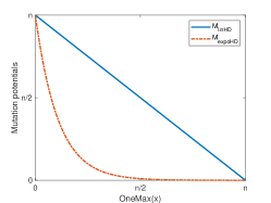
Figure 1. Mutation potentials with respect to the distance to the optimum of OneMax. Since fitness values and Hamming distance are the same for OneMax, we only plot one exponentially decaying curve.

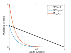
Figure 2. Mutation potentials for LeadingOnes . Expected values are provided for IPHs that use Hamming distance.

In this section we evaluate the performance of the different inversely proportional mutation potentials, assuming the optimum is known (i.e., $best=opt$). Under this assumption, the operators exhibit their ideal behaviour (i.e., the mutation potential decreases with the desired rate as the optimum is approached). Our aim is to evaluate what speed-ups can be achieved in ideal conditions compared to the well-studied static mutation potentials. To achieve such comparisons we perform runtime analyses of the (1+1) IA^hyp using the IPHs on the OneMax and LeadingOnes unimodal benchmark functions for which the performance of the same algorithm using static mutation potentials is known (Corus et al., 2017). The simple to define OneMax function counts the number of 1-bits in the bit string and is normally used to show the hill climbing ability of the algorithm. On the other hand, LeadingOnes, is a more complicated unimodal problem which counts the consecutive number of 1-bits at the beginning of the bit string before the first 0-bit.

The pseudo-code of the algorithm, $(1+1)\text{IA}^{\text{Hyp}}$ , is given in Algorithm 1. It simply uses one candidate solution in each iteration to which inversely proportional hypermutations are applied. The results proven in this section and comparisons with static hypermutations are summarised in Table 1. As previously mentioned, Constructive mutation in Algorithm 1 is a mutation step where the evaluated bit string is at least as fit as its parent.

Figures 1 and 2 show how the studied mutation potentials decrease during the run of the algorithm when optimising OneMax and LeadingOnes, respectively.

Algorithm 1 $(1+1)$ IA^Hyp 

1:  Initialise $x\in\{0,1\}^{n}$ uniformly at random;

2:  Evaluate $f(x)$;

3:  while termination condition is not satisfied do

4:      $M=IPM(x)$;

5:     Create $y$ by flipping at most $M$ distinct bits of $x$ selected uniformly at random one after another until a constructive mutation happens;;

6:     if $f(y)\geq f(x)$ then

7:        $x:=y$.

3.1. OneMax

The following three theorems derive the expected runtimes of the three variants of IPM for the function $\textsc{OneMax}(x):=\sum_{i=1}^{n}x_{i}$. By decreasing the potential linearly with the decrease of the Hamming distance, a logarithmic factor may be shaved off from the expected runtime of the $(1+1)$ IA^Hyp compared to the expected runtime if static hypermutation potentials were used.

The following lemma, called Ballot theorem, is used throughout this paper to derive lower bounds on the runtime of the algorithms for OneMax$(x):=\sum_{i=1}^{n}x_{i}$. It was first used to analyse hypermutations with mutation potential for the same function by Jansen and Zarges (Jansen and Zarges, 2011b). This theorem is essentially used to show the probability of picking more 1-bits than 0-bits during one hypermuation operation given that there are more 1-bits in the initial bit-string (or vice-versa).

Lemma 3.1 (Ballot Theorem (Feller, 1968)).

In a ballot, suppose that candidate P receives $p$ votes and candidate Q receives $q$ votes, such that $p>q$. The probability that throughout the counting P is always ahead of Q is $(p-q)/(p+q)$.

Theorem 3.2.

The $(1+1)$ IA^Hyp using M${}_{\text{linHD}}$ optimises OneMax in $\Theta(n^{2})$ expected fitness function evaluations.

Proof.

Considering $i$ as the number of 0-bits in the candidate solution, the probability of improvement in the first step is $i/n$. Knowing that at most $n$ improvements are needed to find the optimum and in case of failure $H(x,opt)=i$ fitness function evaluations will be wasted, the total expected time to optimise OneMax is at most $\sum_{i=1}^{n}\frac{n}{i}\cdot i=O(n^{2})$.

In order to prove a lower bound, we use Ballot theorem (Feller, 1968) which is stated in Lemma 3.1. By Chernoff bounds the number of 0-bits in the initialised solution is at least $n/3$ w.o.p. Considering the number of 0-bits as $i=q$ and the number of 1-bits as $n-i=p$, the probability of an improvement is at most $1-(p-q)/(p+q)=1-(n-2i)/n=2i/n$ by Lemma 3.1 where $i=H(x,opt)$. This means that we need to wait at least $n/(2i)$ iterations to see an improvement and each time the mutation operator fails to improve the fitness, $i$ fitness function evaluations will be wasted. Considering that at least $n/3$ improvements are needed, the expected time to optimise OneMax is larger than $\sum_{i=1}^{n/3}\frac{n}{2i}\cdot i=\Omega(n^{2})$. ∎

The following theorem shows that a greater speed up may be achieved if the potential decreases exponentially rather than linearly. Its proof deviates from the proof of Theorem 3.2 only in the amount of wasted evaluations. Note that for OneMax the Hamming distance of a solution to the optimum and its difference in fitness are the same. Hence, the subsequent corollary is obvious.

Theorem 3.3.

The $(1+1)$ IA^Hyp using M${}_{\text{expoF(x)}}$ optimises OneMax in $O(n^{3/2+\epsilon}\log n)$ and $\Omega(n^{3/2-\epsilon})$ expected fitness function evaluations for any arbitrarily small constant $\epsilon>0$.

Corollary 3.4.

The $(1+1)$ IA^Hyp using M${}_{\text{expoHD}}$ optimises OneMax in $O(n^{3/2+\epsilon}\log n)$ and $\Omega(n^{3/2-\epsilon})$ expected fitness function evaluations for any arbitrarily small constant $\epsilon>0$.

3.2. LeadingOnes

In the previous section it was shown that decreasing the mutation rate linearly with the Hamming distance to the optimum gave a small improvement for OneMax. The following theorem shows that no improvement over static mutation potentials are achieved for LeadingOnes$:=\sum_{i=1}^{n}\prod_{j=1}^{i}x_{i}$. The main reason for the lack of asymptotic improvement is that a linear mutation potential is sustained until at least a linear number of improvements are achieved.

Theorem 3.5.

The $(1+1)$ IA^Hyp using mutation potential M${}_{\text{linHD}}$ optimises LeadingOnes in $\Theta(n^{3})$ expected fitness function evaluations.

Proof.

The probability of improvement in each step is at least $1/n$ which is the probability of flipping the leftmost 0-bit. As at most $n$ improvements are needed and each failure in improvement yields $n$ wasted fitness function evaluations (as the $H(x,opt)$ is at most $n$), the expected time to find the optimum is at most $\sum_{i=1}^{n}n\cdot n=O(n^{3})$.

The proof for lower bound is the same as the proof of Theorem 3.6 in (Corus et al., 2017) for the expected runtime of the $(1+1)~{}IA^{Hyp}_{\geq}$ with the exception that the wasted amount of fitness function evaluations in case of failure is now $H(x,opt)$ instead of $n$.

Considering $i$ as the number of leading 1-bits, we show the expected number of fitness function evaluations until an improvement happens by $E(f_{i})$. Any candidate solution has $i$ leading 1-bits with a 0-bit following, and then $n-i-1$ other 0-bits and 1-bits which are distributed uniformly at random (Droste et al., 2002). We take into account three possible events of $E_{1}$, $E_{2}$ and $E_{3}$ that can happen in the first bit flip; $E_{1}$ is the event of flipping a leading 1-bit which happens with probability $i/n$, $E_{2}$ is the event of flipping the first 0-bit which happens with probability $1/n$, and $E_{3}$ which is the event of flipping any other bit which happens with probability $(n-i-1)/n$. So we get $E(f_{i}|E_{1})=E[H(x,opt)]+E(f_{i})$ , $E(f_{i}|E_{2})=1$, and $E(f_{i}|E_{3})=1+E(f_{i})$. With law of total expectation and considering that the expected value of $H(x,opt)$, i.e, $E[H(x,opt)]$, is $(n-i)/2+\epsilon n$, we get $E(f_{i})=\frac{i}{n}\left(\frac{n-i}{2}+\epsilon n+E(f_{i})\right)+\frac{1}{n}\cdot 1+\frac{n-i-1}{n}\left(1+E(f_{i})\right)$. Solving it for $E(f_{i})$ gives us $E(f_{i})=\frac{in-i^{2}+2n-2i+2\epsilon i}{2}$. We know that the expected number of consecutive 1-bits that follow the leftmost 0-bit is less than two (Droste et al., 2002) which means the probability of not skipping a level $i$ is $\Omega(1)$. The initial solution on the other hand will have more than $n/2$ leading ones with probability at most $2^{-n/2}$. Thus, we obtain a lower bound $(1-2^{-n/2})\sum_{i=n/2}^{n}E(f_{i})=\Omega(1)\sum_{i=n/2}^{n}\frac{in-i^{2}+2n-2i+2\epsilon i}{2}=\Omega(n^{3})$ on the expectation. ∎

The following two theorems show that exponential fitness-based mutation potential gives us at least a logarithmic and at most $\sqrt{n}$ factor speed-up compared to static mutation potentials. Before proving the main results, we introduce the following lemma that will be used in the proof of upcoming theorems.

Lemma 3.6.

For large enough $n$ and any arbitrarily small constant $\epsilon$, $n^{1/n^{\epsilon}}=(1+\frac{\ln{n}}{n^{\epsilon}})(1\pm o(1))$.

Proof.

By raising $\left(1+\frac{\ln{n}}{n^{\epsilon}}\right)$ to the power of $\frac{n^{\epsilon}}{\ln{n}}\cdot\frac{\ln{n}}{n^{\epsilon}}$ we have $\left(1+\frac{\ln{n}}{n^{\epsilon}}\right)^{\frac{n^{\epsilon}}{\ln{n}}\cdot\frac{\ln{n}}{n^{\epsilon}}}=\left(1\pm o(1)\right)e^{\frac{\ln{n}}{n^{\epsilon}}}=(1\pm o(1))n^{1/n^{\epsilon}}.$∎

Theorem 3.7.

The $(1+1)$ IA^Hyp using M${}_{\text{expoF(x)}}$ optimises LeadingOnes in $O(n^{3}/\log n)$ and $\Omega(n^{5/2+\epsilon})$ expected fitness function evaluations for any arbitrarily small constant $\epsilon>0$.

Proof.

The expected number of leading 1-bits is less than two in the initialised bit string. The probability of improvement in the first step is $1/n$. In case of failing in improving at the first step, at most $n^{\frac{n-i}{n}}$ fitness function evaluations would get wasted with $i$ showing the number of leading 1-bits. Therefore, the total expected time to find the optimum is $E(T)\leq\sum_{i=1}^{n}n\cdot n^{(n-i)/n}=O(n^{3}/\log n)$ considering that $\sum_{i=1}^{n}n^{(i)/n}\leq\sum_{i=0}^{\infty}(n^{1/n})^{i}=1/(1-n^{i})$ which is $n^{2}/(\log n)$ by Lemma 3.6.

The proof for lower bound is similar to the proof of Theorem 3.5, except in the calculation of $E(f_{i})$ when we want to consider the amount of wasted fitness function evaluations in case of $E_{1}$ happening. Here we have $E(f_{i})=\frac{i}{n}\left(n^{(n-i)/n}+E(f_{i})\right)+\frac{1}{n}\cdot 1+\frac{n-i-1}{n}\left(1+E(f_{i})\right)$. Solving it for $E(f_{i})$ gives us $E(f_{i})=in^{i/n}+n-i$. Hence the expected time to optimise LeadingOnes is $(1-2^{-n/2})\sum_{i=n/2}^{n}E(f_{i})=\Omega(1)\sum_{i=1}^{n/2-\epsilon n/2}in^{(n-i)/n}+n-i=\\ \Omega(1)\left(\sum_{i=1}^{n/2-\epsilon n/2}n-i+\sum_{i=1}^{n/2-\epsilon n/2}in^{(n-i)/n}\right)$. Evaluating the second sum in the interval $i\in[n/2-\epsilon n/2,n/2-\epsilon]$, we get $\epsilon n/2\cdot(n/2-\epsilon n)\cdot n^{1/2-\epsilon}=\Omega(n^{5/2-\epsilon})$. ∎

An advantage of Hamming distance-based exponential decays of the mutation potential compared to fitness-based ones are provided by the following theorem for LeadingOnes. The reason can be appreciated from Fig. 2. While the initial fitness is very low, hence the potential is very high, the actual number of bits that have to be flipped to reach the optimum is much smaller. M${}_{\text{expoHD}}$ exploits this property, thus wastes less fitness evaluations than M${}_{\text{expoF(x)}}$ . .

Theorem 3.8.

The $(1+1)$ IA^Hyp using M${}_{\text{expoHD}}$ optimises LeadingOnes in $O(\frac{n^{5/2+\epsilon}}{\ln n})$ and $\Omega(n^{9/4-\epsilon})$ expected fitness function evaluations for any arbitrarily small constant $\epsilon>0$.

Given that M${}_{\text{expoHD}}$ provides larger speed-ups compared to the other IPH operators and is stable to the scaling of fitness functions, we will use it in the remainder of the paper.

4. Realistic Inefficient Behaviour

In this section we consider the usage of M${}_{\text{expoHD}}$ in realistic applications where the optimum is unknown. To this end the best found solution will be used by the operator rather than the unknown optimum. We combine M${}_{\text{expoHD}}$ with hybrid ageing, as in the Opt-IA AIS and call it $(1+1)$ Opt-IA (Cutello et al., 2007). It’s pseudo-code is provided in Algorithm 2. Ageing has been shown to enable algorithms to escape from local optima either by identifying a gradient leading away from it or by restarting the whole optimisation process.

Our aim is that the more local optima are identified by the algorithm, the more M${}_{\text{expoHD}}$ approximates its ideal behaviour. However, we will show that this is not the case using the well-studied bimodal benchmark functions TwoMax (4) (Friedrich et al., 2009; Sudholt, 2019; Oliveto et al., 2018; Osuna and Sudholt, 2017) as an example:

(4) $$\textsc{TwoMax}:=\max\left\{\sum_{i=1}^{n}x_{i},\;n-1\sum_{i=1}^{n}x_{i}\right\}$$

The function is usually used to evaluate the global exploration capabilities of evolutionary algorithms i.e., whether the populations identify both optima of the function. Our analysis shows that once the $(1+1)$ Opt-IA escapes from one local optima, the mutation rate will increase as the algorithm climbs up the other branch. As a result the algorithm struggles to identify the other optimum and wastes more and more fitness function evaluations as it approaches it. Thus, defeating the whole purpose behind IPH.

On the bright side, we will show that M${}_{\text{expoHD}}$ combined with ageing can escape from local optima. We will use the well known Cliff function for the purpose where static hypermutations are inefficient because due to their high mutation rates, even if they escape, they jump back to the local optima with high probability. Cliff is defined as follows:

(5) $$\textsc{Cliff}_{k}(x)=\begin{cases}\sum_{i=1}^{n}x_{i}&\text{if}\;\sum_{i=1}^{n}x_{i}\leq n-k,\\ \sum_{i=1}^{n}x_{i}-k+1/2&\text{otherwise.}\end{cases}$$

Both bimodal functions are illustrated in Fig 3.

Among the different varaints of ageing, hybrid ageing has been shown to be very efficient at escaping local optima (Oliveto and Sudholt, 2014; Corus et al., 2017, 2018). Using this operator, the individual is assigned with an initial $age=0$. During each iteration of the algorithm the age increases by 1 and is passed to the offspring if the offspring does not improve over its parent’s fitness. If the offspring is better than the parent, then its age is set to 0. At the end of each iteration any individual with age larger than a threshold ($\tau$) is removed with probability $1/2$ and in case there is no other individual left in the population, a new individual is initialised uniformly at random.

Algorithm 2 $(1+1)$ Opt-IA with M${}_{\text{expoHD}}$ 

1:  Initialise $x\in\{0,1\}^{n}$ uniformly at random and add to $P$;

2:  Set $best=x$;

3:  Evaluate $f(x)$;

4:  Set $x.age=0$;

5:  while termination condition is not satisfied do

6:     $x.age=x.age+1$;

7:      $M=$M${}_{\text{expoHD}}$ ;

8:     Create $y$ by flipping at most $M$ distinct bits of $x$ selected uniformly at random one after anotherther until a constructive mutation happens;

9:     If $f(y)>f(x)$, then $y.age=0$. Else, $y.age=x.age$;

10:     If $f(y)\geq f(best)$, then set $best=y$

11:     Add $y$ to $P$;

12:     For $x$ and $y$ in $P$, if $age\geq\tau$ then remove the individual with probability $1/2$;

13:     Select the best individual in $P$ and remove the other;

14:     If $|P|=0$, create $x\in\{0,1\}^{n}$ uniformly at random and add to $P$;

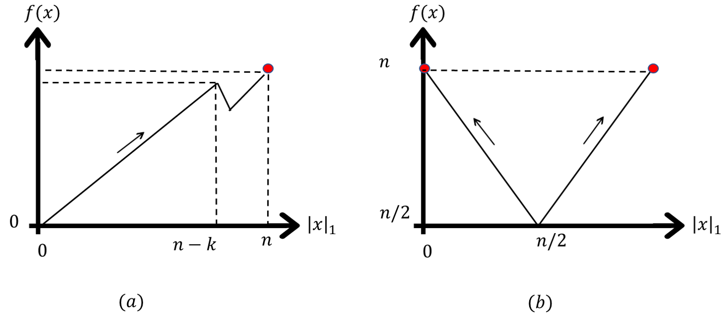
Figure 3. (a) Cliff and (b) TwoMax test functions

The following theorem shows that after the algorithm escapes from the local optimum the mutation rate increases as the algorithm climbs up the opposite branch. This behaviour causes a large waste of fitness evaluations defying the objectives of IPH.

Theorem 4.1.

The expected runtime of Algorithm 2 with M${}_{\text{expoHD}}$ to optimise TwoMax is $O(n^{2}\log n)$ with $\tau=\Omega(n^{1+\epsilon})$ for some constant $\epsilon>0$.

Proof.

Let $x_{t}$ be the current solution at the beginning of the iteration $t$. Immediately after the initialisation, the ’best’ seen is the current individual $x_{1}$ itself and the mutation potential is $M=M_{expoHD}=n^{HD(x_{1},x_{1})/n}=n^{0}=1$. Note that $x_{t}\neq x_{t+1}$ if and only if either $f(x_{t+1})\geq f(x_{t})$ or $x_{t+1}$ is reinitialised after $x_{t}$ is removed from the population due to ageing. Thus, the mutation operator flips a single bit at every iteration until ageing is triggered for the first time. The improvement probability will be at least $1/n$ until either $1^{n}$ or $0^{n}$ is sampled. Given that the ageing threshold $\tau$ is at least $n^{1+\epsilon}$ for some constant $\epsilon>0$, the probability that the current solution will not improve $\tau$ times consecutively is at most $(1-\frac{1}{n})^{n^{1+\epsilon}}$ $e^{-\Omega(n^{\epsilon})}$. Hence, with overwhelmingly high probability, the first optimum will be found before ageing is triggered. Given that the ageing operator is not triggered, the expected time to find the first optimum is at most $O(n\log{n})$ as for the standard $(1+1)~{}\text{RLS}_{1}$ . After finding the first optimum, no single-bit flip can yield an equally fit solution. The individual then reaches age $\tau$ and the ageing reinitialises the current solution. Thus, with $\left(1-2^{n}\right)\cdot\left(1-e^{-\Omega(n^{\epsilon})}\right)$ probability a new solution will be initialised in $O(n\log{n})+\tau+n$ and the current best will be the first discovered optimum. Let the first and second branch denote the subsets of the solution space which consist of solutions with less than and more than Hamming distance $n/2$ to the first discovered optimum respectively.

We first consider the case if the reinitialised solution is on the first branch. Given that the current solution has fitness $i$, the distance to the best seen is $n-i$ and the mutation potential is $M=n^{\frac{n-i}{n}}$. Since, the first constructive mutation ensures that the probability of improvement is always at least $1/n$, with overwhelmingly high probability the ageing will not be triggered until either optimum is discovered. Thus, given that the current solution is always on the first branch, the proof of Theorem 3.4 carries over and the expected time to find the first discovered optimum once again is at most $O(n^{3/2}\log{n})$ in expectation. When the first discovered optimum is sampled again, with overwhelming probability, the current solution is reinitialised with the first discovered optimum as the best seen solution in at most $\tau+n$ iterations.

Now, we consider the case where the current solution is on the second branch. A lower bound on the probability that the current solution will reach the optimum of the second branch before sampling an improving solution in the first branch will conclude the proof since the expected time to do so is $O(n^{3/2}\log{n})$ given that the current solution does not switch branches before.

We will start by bounding the mutation potential for a solution in the second branch with fitness value $n-k$. Since the M${}_{\text{expoHD}}$ is always smaller than M${}_{\text{linHD}}$ , we can assume that no more than $n-k$ bits will be flipped.

Without losing generality, let the second branch be the branch with more 0-bits. We will now consider the final solution sampled by the hypermution operator since it has the highest probability of finding a solution with at least $n-k$ 1-bits (i.e., switching to the first branch). The current solution has $n-k$ 0-bits and $k$ 1-bits. If more than $k/2$ 1-bits are flipped, then the number of $1$s in the final solution after $n-k$ mutation steps is less than $n-k$ since the number of $0$s flipped to $1$s is less than $n-k-k/2$ and the number of remaining 1-bits is less than $k/2$. The event that at most $k/2$ 1-bits are flipped is equivalent to the event that in a uniformly random permutation of the $n$ bit positions at least $k/2$ $1$-bits are ranked in the last $k$ positions of the random permutation. We will now bound the probability that exactly $k/2$ $1$-bits are in the last $k$ position since having more has a smaller probability. Each particular outcome of the last $k$ positions has the equal probability of $\prod_{i=0}^{k-1}(n-i)^{-1}$. There are $\binom{k}{k/2}$ different equally like ways to chose $k/2$ $1$-bits and $k!$ different permutations of the last $k$ positions thus the probability of having exactly $k/2$ 1-bits in the last $k$ positions is: $\prod\limits_{i=0}^{k-1}\frac{1}{n-i}\cdot\binom{k}{k/2}\cdot k!=\prod\limits_{i=0}^{k-1}\frac{1}{n-i}\cdot\left(\frac{k!}{(k/2)!}\right)^{2}<\left(\frac{k}{n-k}\right)^{k}$. For any $k\in[4,\frac{n}{2}-\Omega(\sqrt{n})]$ this probability is in the order of $\Omega(1/n^{4})$. Using union bound over the probabilities of having more than $k/2$ $1$-bits and the probabilities of improving before the final step, we obtain an $\frac{k}{2}\cdot(n-k)\cdot\Omega(1/n^{4})=\Omega(1/n^{2})$. Since the new solutions are uniformly sampled, the number of bits in the solutions are initially distributed binomially with parameters $n$ and $1/2$ which has a variance in the order of $\Theta(\sqrt{n})$ and implies that with constant probability $k<\frac{n}{2}-\Omega(\sqrt{n})$ in the initial solution. Given that the expected time in terms of generations is in the order of $O(n\log{n})$, the total probability of switching branches while $k\in[k,\frac{n}{2}-\Omega(\sqrt{n})]$ is at most $\left(1+1/n^{2}\right)^{O(n\log{n})}=1-\Omega(1)$. Finally, we will consider the cases of $k\in\{1,2,3\}$ separately. When $k=1$, the probability of flipping less than $k/2$ 1-bits is equivalent to the probability of not flipping the single 1-bit which happens with probability $1/n$. For $k=2$, similarly we have to flip at most one 1-bit with probability $O(1/n)$. For $k=3$, it is necessary that at least two 1-bits are not flipped which happens with probability at most $O(1/n^{2})$ probability. Thus, the probability of switching branches when $k<4$ is at most $O(1/n)$, which lower bounds the total probability of switching branches in the order of $1-\Omega(1)$ given that the initial solution has at least $k>\frac{n}{2}-\Omega(\sqrt{n})$ 1-bits (which also occurs with at least $\Omega(1)$ probability). Given that no switch occurs, the expected time to find the second optimum is $\sum_{i=1}^{n/2+\epsilon n}\frac{n}{i}\cdot n^{\frac{n-i}{n}}=n^{2}\sum_{i=1}^{n/2-\epsilon n}\frac{1}{i}\cdot n^{\frac{-i}{n}}<n^{2}\sum_{i=\epsilon n}^{2\epsilon n}\frac{1}{2n}\cdot n^{\frac{-i}{n}}<$ at most $O(n^{2}\log{n})$ as $n^{-i/n}\leq(1-\ln{n}/n)$ for all $i$. ∎

Now we show that, differently from static hypermutations M${}_{\text{expoHD}}$ combined with ageing can escape from the local optima of Cliff, hence optimise the function efficiently.

Theorem 4.2.

Algorithm 2 with M${}_{\text{expoHD}}$ and $\tau=\Omega(n^{1+\epsilon})$ for an arbitrarily small constant $\epsilon$ optimises Cliff_k with $k<n(\frac{1}{4}-\epsilon)$ and $k=\Theta(n)$ in $O(n^{3/2}\log{n}+\tau n^{1/2}+\frac{n^{7/2}}{k^{2}})$ fitness function evaluations.

Proof.

The analysis will follow a similar idea to the proof of Theorem 4.1. After initialisation the initial mutation potential is $M=1$ since the current solution is the best seen solution. With single bit-flips it takes in expectation at most $O(n)$ to find on the local optima of the cliff (a search point with $n-k$ 1-bits) as the improvement probability is always at least $(n-k)/n=\Omega(1)$. Since the local optima cannot be improved with single bit flips, in $\tau$ generations after it was first discovered the ageing will be triggered and in the following $n$ steps the current solution will be removed from the population due to ageing with probability at least $1-2^{-n}$. Hamming distance of the reinitialised soluton will be distributed binomially with parameters $n$ and $1/2$ and with overwhelmingly high probability will be smaller than $n/2+n^{2/3}$, yielding an initial mutation potential of $M=\Omega(n^{1/2})$. We pessimistically assume that the mutation potential will not decrease until the local optima is found again, which implies that the expected time will be at most $O(n^{3/2}\log{n}+\tau n^{1/2})$ since each iteration will waste an extra $\Omega(n^{1/2})$ fitness function evaluations. After finding a local optima again, the mutation potential will be $M=1$ since it will replace the previously observed local optima as the best seen. The process of reinitialisation and reaching the local optima will repeat itself until the following event happens.

If the local optima produces an offspring with $n-k+1$ bits with probability $k/n$ and if this solution survives the ageing operator with probability $(1-p_{die})$, then the reinitialised solution will be rejected since its fitness value is less than $n-k$ with overwhelming probability. The Hamming distance of this new solution to the best seen will be exactly one since it is created via a single bit-flip, thus itsmutation potential will be $M=1$. Moreover, if the surviving offspring improves again with proability $(k/n)$ in the next iteration, it will reset its age to zero and will have Hamming Distance at least two to any local optima. In expected $O(n/\log{n})$ iterations (not function evaluations), this solution will reach the global optimum unless a solution with less than $n-k$ 1-bits is sampled before. Initially this will be impossible since $M=1$ for at least $\omega(1)$ more steps and later $M<3$ as long as the distance to the last seen local optima is at most $n/\ln{n}$ since $n^{\frac{n/\ln{n}}{n}}=e$. Note that the number of $1$s does not always reflect the actual Hamming distance since more than one bit can be flipped in an accepted offspring. We will pessimitically assume that all improvements has increased the Hamming distance by three until the total Hamming distance reaches $n/\ln{n}$, which implies that there has been $n/(3\ln{n})$ accepted solutions. Ballot theorem implies that sampling a solution at least as good as the parent (which are the only solutions that are accepted) has probability at most $2i/n$ where $i$ is the number of 0-bits in the solution. Since the probability of improving in the first step is at least $i/n$, we can conclude that the conditional probability that an accepted offspring is an improvement is at least $1/2$. Thus, when the Hamming distance to the local optima reaches $n/\ln{n}$, in expectation the current solution will have at least $n/(6\ln{n})$ extra 1-bits compared to the local optima and at least $n^{3}/5$ extra bits with overwhelmingly high probability. The Hamming distance to the local optima can be at most $2k$ since both the local optima and the current solution have less than $k$ 0-bits. Since $k<n/4$ the the mutation potential is at most $\sqrt{n}$, thus, no hypermutation can yield a solution with less than $n-k+2$ 1-bits. Therefore, once a solution with $n-k+2$ bits is added to the population the algorithm finds the optimum with overwhelming probability in $O(n\log{n})$ iterations and in at most $O(n^{3/2}\log{n})$ fitness functions evaluations since the the mutation potential is at most $\sqrt{n}$. The probability of obtaining a solution with $n-k+2$ 1-bits at the end of each cycle of reinitialisation and removal of the local optima due to ageing is $(1-p_{die})(k/n)^{2}$. Since each such cycle takes $O(n^{3/2})$ fitness function evaluations our claim follows. ∎

5. An Efficient Opt-IA with IPH

In the previous section we observed in the analyses of both Cliff and TwoMax that towards the end of the optimisation process the mutation potential increases as the current solution approaches an undiscovered, potentially promising optimum. This behaviour is against the design intentions of the inversely proportional mutation potential since in the final part of the optimisation process it gets harder to find improvements and high mutation potentials lead to many wasted fitness function evaluations. The underlying reason of this behaviour in both Cliff and TwoMax landscapes was the necessity to follow a gradient away from the local optimum for finding the global one. Considering that this necessity would be ubiquitous in optimisation problems we propose a new method to control mutation potentials in this section. Algorithm 3 uses a mutation potential inversely proportional to the current solution’s Hamming distance to its origin, where the origin is defined as the ancestor of the current bitstring after the last removal of a solution due to ageing. We call the newly proposed mutation operator Symmetric M${}_{\text{expoHD}}$ . This mutation potential reliably decreases (at the same rate it would use if it was approaching the currently best seen local optimum) as the current solution improves and moves away from its origin up until it starts doing local search and finds a local optimum. Every time a local optimum is found, ageing is triggered after approximately $\tau$ steps and then both surviving and reinitialised individuals reset their origin to their own bitstring.

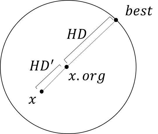
Figure 4. The geometric representation of the mutation potential of Algorithm 3. The mutation potential is determined according to the ratio of the Hamming distance between the current solution and its origin and the Hamming distance between its origin and the best seen solution.

Algorithm 3 (1+1) Opt-IA with Symmetric M${}_{\text{expoHD}}$ 

1:  Set $x\sim Unif(\{0,1\}^{n})$

2:  Set $x.origin:=x$, $x.age:=0$; $Best:=x$

3:  Evaluate $f(x)$;

4:  while termination condition not satisfied do

5:     $x.age:=x.age+1$;

6:     Create $y$ by flipping at most $M:=\left\lceil n\cdot n^{-\frac{HD\left(x,x.org\right)}{\max\{HD\left(Best,x.org\right),1\}}}\right\rceil$ distinct bits of $x$ selected uniformly at random one after another until a constructive mutation happens;

7:     $y.origin:=x.origin$;

8:     if $f(y)>f(x)$ then

9:        $y.age:=0$;

10:        if $f(y)\geq Best$ then

11:           $Best:=y$;

12:     else

13:        $y.age:=x.age$;

14:     for $win\{x,y\}$ do

15:        if  $w.age>\tau\wedge p_{die}=1/2>R\sim Unif(0,1)$ then

16:           Set $w\sim Unif(\{0,1\}^{n})$ , $w.age=0$,

17:           Set $x.origin=x$, $y.origin=y$

18:     Set $x=\arg\max\limits_{z\in\{x,y\}}f(z)$;

The following theorem shows that once one local optimum has been identified the mutation potential of Symmetric M${}_{\text{expoHD}}$ decreases as both optima are approached as desired and the wished for speed-up in the runtime is achieved.

Theorem 5.1.

The Algorithm 3 with $\tau=\Omega(n^{1+\epsilon})$ for any arbitrarily small constant $\epsilon>0$ has expected runtime of $O(n^{3/2}\log{n})$ on TwoMax.

Proof.

The expected time until the first branch is optimised is $O(n\log{n})$ since the best seen search point is the current best individual and consequently the mutation potential is $M=1$. Since the improvement probability is at least $1/n$ and $\tau=\Omega(n^{1+\epsilon})$, the ageing operator does not trigger before finding one of the optima with overwhelming probability. Once one of the optima is found, the ageing reinitialises the individual while the first discovered optima stays as the current best seen search point. For the randomly reinitialised solution, the Hamming distance to the best seen binomially distributed with parameters $n$ and $1/2$. Using a Chernoff bound we can bound the distance to the previously seen optima by at most $n/2+n^{2/3}$ with overwhelmingly high probability. This Hamming distance implies an initial mutation potential of $M<n^{\frac{\frac{n}{2}+n^{2/3}}{n}}=n^{\frac{1}{2}+\frac{1}{n^{1/3}}}$ which decreases as the individual increases its distance to the origin and can never go above its initial value where the distance is zero. Pessimistically assuming that the mutation potential will be $n^{\frac{1}{2}+\frac{1}{n^{1/3}}}=O(n^{1/2})$ throughout the run, we can obtain the above upper bound by summing over all levels and using coupon collector’s argument. ∎

The following theorem shows that Symmetric M${}_{\text{expoHD}}$ is also efficient for Cliff

Theorem 5.2.

The Algorithm 3 with $\tau=\Omega(n^{1+\epsilon})$ has expected runtime of $O(n^{3/2}\log{n}+\tau n^{1/2}+\frac{n^{7/2}}{k^{2}})$ on Cliff_k.

Proof.

The proof of the result is almost identical to the proof of Theorem 4.2. The most important distinction is that once a solution with $n-k+2$ is created its mutation potential remains at $M=1$ until it finds the global optimum because when the ageing triggers the surviving solutions all reset their origin to their own bitstring, i.e. start doing randomised local search. ∎

6. Conclusion

We have presented an analysis of Inversely Proportional Hypermutations (IPH). Previous theoretical studies have shown disappointing results concerning the IPH operators from the literature. In this paper we have proposed a new IPH based on Hamming distance and exponential decay. We have shown its effectiveness in isolation for unimodal functions compared to static hypermutations in the ideal conditions when the optimum is known. Furthermore, we have provided a symmetric version of the operator for the complete Opt-IA AIS to be used in practical applications where the optimum is usually unknown. We have proved its efficiency for two well-studied bimodal functions. Future work should evaluate the performance of the proposed algorithm for combinatorial optimisation problems with practical applications.

Acknowledgments: The research leading to these results has received funding from the EPSRC under grant agreement no
EP/M004252/1.

Appendix A Appendix

Proof of Theorem 3.3

Proof.

By Chernoff bounds, the initialised solution has at most $n/2+\epsilon n$ 0-bits w.o.p for any arbitrary small $\epsilon=\Theta(1)$. The probability of improvement in the first mutation step is at least $i/n$ with $i$ showing the number of 0-bits. As we need at most $n/2+\epsilon n$ improvements and each time the mutation fails to make an improvement at least $n^{1-\frac{n-i}{n}}$ fitness function evaluation would get wasted, the total expected time to find the optimum will be $E(T)\leq\sum_{i=1}^{n/2+\epsilon n}\frac{n}{i}\cdot n^{\frac{i}{n}}\leq n^{3/2+\epsilon}\log n$. To prove the lower bound, consider $i$ as the number of 0-bits. By Chernoff bounds, $i$ is at least $n/2-\epsilon n$ 0-bits in the initialised bit string. The number of wasted fitness function evaluations at each failure is $n^{\frac{i}{n}}$. If we consider the time spent between levels $n(1/2+\epsilon/2)$ and $n(1/2+\epsilon)$, we get the expected time of $n^{\frac{n/2-\epsilon n}{n}}\cdot\sum_{i=n/2+n\epsilon/2}^{n/2+\epsilon n}\Omega(1)=n^{1/2-\epsilon}\cdot\epsilon n/2\cdot\Omega(1)=\Omega(n^{3/2-\epsilon})$.

∎

Proof of Theorem 3.8

Proof.

The proof is similar to the proof of Theorem 3.5 however each failure in improvement yields $n^{HD/n}$ wasted fitness function evaluations. The expected time to find the optimum is at most $\sum_{i=1}^{n}n\cdot n^{HD/n}$ with $i$ showing the number of leading 1-bits. Knowing that the bits after the leading ones are uniformly distributed, by Chernoff bounds the number of 0-bits (Hamming distance to the $opt$) is less than $1/2(n-i)+\epsilon n$ w.o.p. Hence, the expected time to optimise LeadingZeros is $\sum_{i=1}^{n}n\cdot n^{\frac{1/2(n-i)+\epsilon n}{n}}=n\sum_{i=1}^{n}n^{\frac{1}{2}-\frac{i}{2n}+\epsilon}=n\cdot n^{1/2+\epsilon}\sum_{i=1}^{n}n^{-\frac{i}{2n}}$. Knowing that $\sum_{i=0}^{\infty}n^{-\frac{i}{2n}}=\frac{1}{1-n^{(-1/n)}}$ and $n^{-1/n}\leq\left(1-\frac{\ln n}{n}\right)(1-o(1))$ (Lemma 3.6) , we get $1-n^{(-1/n)}\leq\frac{n}{\ln n}(1+o(1))$. Hence, the expected time is $E(T)\leq n^{3/2+\epsilon}\cdot O(\frac{n}{\ln n})=O(\frac{n^{5/2+\epsilon}}{\ln n})$.

The proof for lower bound is similar to the proof of Theorem 3.5. Here we have $E(f_{i})=\frac{i}{n}\left(n^{HD/n}+E(f_{i})\right)+\frac{1}{n}\cdot 1+\frac{n-i-1}{n}\left(1+E(f_{i})\right)$. Replacing $HD$ with $(n-i)/2-\epsilon n$ and then solving this equation for $E(f_{i})$ gives us $E(f_{i})=in^{1/2-\epsilon-i/(2n)}+n-i$. Then, we get the expected runtime of

$$(1-2^{-n/2})\sum_{i=n/2}^{n}E(f_{i})\geq\Omega(1)\sum_{i=n/2-\epsilon n}^{n/2-\epsilon n/2}\left(in^{1/2-\epsilon-i/(2n)}+n-i)\right)$$

$$\geq\Omega(1)\sum_{i=n/2-\epsilon n}^{n/2-\epsilon n/2}\left(in^{1/4-\epsilon}\right)=\Omega(n^{9/4-\epsilon}).$$

∎

References

- (1)
- Brownlee (2007) Jason Brownlee. 2007. Clonal Selection Algorithms. Technical Report. Complex Intelligent Systems Laboratory (CIS), Swinburne University of Technology. Techincal report.
- Burnet (1959) Frank M. Burnet. 1959. The Clonal Selection Theory of Acquired Immunity. Cambridge University Press.
- Castro et al. (2002) Leandro Nunes Castro, Leandro Nunes de Castro, and Jonathan Timmis. 2002. Artificial Immune Systems: A New Computational Intelligence Approach. Springer Science and Business Media.
- Corus et al. (2017) Dogan Corus, Pietro S. Oliveto, and Donya Yazdani. 2017. On the Runtime Analysis of the Opt-IA Artificial Immune System. In Proc. of GECCO 2017. 83–90.
- Corus et al. (2018) Dogan Corus, Pietro Simone Oliveto, and Donya Yazdani. 2018. Artificial Immune Systems Can Find Arbitrarily Good Approximations for the NP-hard Partition Problem. In Proc. of PPSN 2018. 16–28.
- Cutello et al. (2007) Vincenzo Cutello, Giuseppe Nicosia, Mario Pavone, and Jonathan Timmis. 2007. An Immune Algorithm for Protein Structure Prediction on Lattice Models. IEEE Trans. Evol. Comp. 11, 1 (2007), 101–117.
- Cutello et al. (2006) Vincenzo Cutello, Mario Pavone, and Jonathan Timmis. 2006. An Immune Algorithm for Protein Structure Prediction on Lattice Models. IEEE Trans. Evol. Comp. 10 (2006), 844–861.
- de Castro and Zuben (2002) Leonardo N. de Castro and Fernando J. Von Zuben. 2002. Learning and Optimization Using the Clonal Selection Principle. IEEE Trans. Evol. Comp. 6, 3 (2002), 239–251.
- Droste et al. (2002) Stefan Droste, Thomas Jansen, and Ingo Wegener. 2002. On the Analysis of the (1+ 1) Evolutionary Algorithm. Theor. Comp. Sci. 276, 1-2 (2002), 51–81.
- Feller (1968) William Feller. 1968. An Introduction to Probability Theory and Its Applications. John Wiley & Sons.
- Friedrich et al. (2009) Tobias Friedrich, Pietro Simone Oliveto, Dirk Sudholt, and Carsten Witt. 2009. Analysis of Diversity-Preserving Mechanisms for Global Exploration. Evolutionary Computation 17, 4 (2009), 455–476. https://doi.org/10.1162/evco.2009.17.4.17401
- Horoba et al. (2009) Christian Horoba, Thomas Jansen, and Christine Zarges. 2009. Maximal Age in Randomized Search Heuristics with Aging. In Proc. of GECCO 2009. 803–810.
- Jansen and Zarges (2011a) Thomas Jansen and Christine Zarges. 2011a. On the Role of Age Diversity for Effective Aging Operators. Evolutionary Intelligence 4, 2 (2011), 99–125.
- Jansen and Zarges (2011b) Thomas Jansen and Christine Zarges. 2011b. Variation in Artificial Immune Systems: Hypermutations with Mutation Potential. In Proc. of ICARIS 2011. 132–145.
- Oliveto and Sudholt (2014) Pietro S. Oliveto and Dirk Sudholt. 2014. On the Runtime Analysis of Stochastic Ageing Mechanisms. In Proc. of GECCO 2014. 113–120.
- Oliveto et al. (2018) Pietro S. Oliveto, Dirk Sudholt, and Christine Zarges. 2018. On the benefits and risks of using fitness sharing for multimodal optimisation. Theoretical Computer Science (2018), –. https://doi.org/doi.org/10.1016/j.tcs.2018.07.007
- Oliveto and Witt (2014) Pietro S Oliveto and Carsten Witt. 2014. On the Runtime Analysis of the Simple Genetic Algorithm. Theoretical Computer Science 545 (2014), 2 –19.
- Oliveto and Witt (2015) Pietro S Oliveto and Carsten Witt. 2015. Improved time complexity analysis of the simple genetic algorithm. Theoretical Computer Science 605 (2015), 21–41.
- Osuna and Sudholt (2017) Edgar Covantes Osuna and Dirk Sudholt. 2017. Analysis of the clearing diversity-preserving mechanism. In Proceedings of Foundations of Genetic Algorithms (FOGA 2017). ACM Press, 55–63.
- Sudholt (2019) Dirk Sudholt. 2019. The Benefits of Population Diversity in Evolutionary Algorithms: A Survey of Rigorous Runtime Analyses. In Theory of Randomized Search Heuristics in Discrete Search Spaces, Benjamin Doerr and Frank Neumann (Eds.). Spinger, –. https://arxiv.org/abs/1801.10087.
- Whitley (1989) Darrell Whitley. 1989. The Genitor algorithm and selection pressure: why rank-based allocation of reproductive trials is best. In Proceedings of the Third International Conference on Genetic Algorithms. 116–121.
- Zarges (2008) Christine Zarges. 2008. Rigorous Runtime Analysis of Inversely Fitness Proportional Mutation Rates. In Proc. of PPSN X. 112–122.