Theory of standing spin waves in finite-size chiral spin soliton lattice

Abstract

We present a theory of standing spin wave (SSW) in a monoaxial chiral helimagnet. Motivated by experimental findings on the magnetic field-dependence of the resonance frequency in thin films of CrNb₃S₆[Goncalves et al., Phys. Rev. B 95, 104415 (2017)], we examine the SSW over a chiral soliton lattice (CSL) excited by an ac magnetic field applied parallel and perpendicular to the chiral axis. For this purpose, we generalize Kittel-Pincus theories of the SSW in ferromagnetic thin films to the case of non-collinear helimagnet with the surface end spins which are softly pinned by an anisotropy field. Consequently, we found there appear two types of modes. One is a Pincus mode which is composed of a long-period Bloch wave and a short-period ripple originated from the periodic structure of the CSL. Another is a short-period Kittel ripple excited by space-periodic perturbation which exists only in the case where the ac field is applied perpendicular the chiral axis. We demonstrate that the existence of the Pincus mode and the Kittel ripple is consistent with experimentally found double resonance profile.

I Introduction

Dynamical responses to external probes disclose the nature of collective excitations in condensed matters. Thin ferromagnetic films in this regard have received much attention in recent years due to striking features never seen in bulk samples and have been widely applied to technology.Barman2018

At the same time, recent studies of thin films and micrometer-sized crystals of the monoaxial chiral helimagnet CrNb₃S₆ have exhibited a number of remarkable phenomena thereby making this system highly attractive for spintronic applications. These include detection of the chiral spin soliton lattice (CSL) by using Lorenz microscopy and small-angle electron diffraction,Togawa2012 a sequence of jumps in magnetoresistanceTogawa2013 ; Wang2017 and magnetic soliton confinement.Togawa2015 ; Book2015 It was argued that the discretization effects result from a specific domain structure, 1-$\mu$m-wide grains with different crystallographic structural chirality. In this system, the direction of in-plane magnetic moments is pinned down around the domain boundary.

An obvious consequence of the pinning effect other than quantization of magnetization and magneto-resistance is an emergence of the intrinsic resonance frequency.Kishine2016 Recent report on magnetic resonance in micro-sized crystals CrNb₃S₆Goncalves2017 revealed that the dynamical resonances of the CSL is sensitive to the polarization of the driving microwave field. In the case where the microwave field is applied parallel to the chiral axis, the resonance profile was attributed to excitation of standing spin waves (SSW) Goncalves2018 . On the other hand, when the microwave field is applied perpendicular to the chiral axis, two resonance modes, with the frequency difference being a few GHz, appear across the entire CSL phase. Furthermore, the resonance modes become asymmetric with regards to the directions of a static field applied perpendicular to the chiral axis to stabilize the CSL. Origins of these two prominent features, (1) double resonance and (2) asymmetry, have not been known as yet. This situation naturally motivate us to address a query concerning possible mechanisms.

For this purpose, we start with turning our attention to the theory of ferromagnetic resonance (FMR) in thin films, pioneered by Kittel.Kittel1958 In Kittel’s theory, the surface spins are essentially pinned down by a strong surface anisotropy field. The case of soft pinning was later considered by Pincus.Pincus1960 In the case of soft pinning, the eigenfrequencies of the interior spin wave are required to match the Larmor frequency of the surface spins. This matching condition is given by Davis-Puszkarski equation,Davis1963 ; Puszkarski1973 ; Banavar1978 which leads to allowed values of the wave vector of the spin wave modes.

Since the first observation in permalloy films,Seavey1958 the detection of the SSW has long attracted considerable attention, including manganite films,Lofland1995 magnonic crystals,Mruczkiewicz2013 ferromagnetic bars.Wismayer2012 The SSW has also been regarded as candidates for working media in spintronics, including Co multi-layers,Buczek2010 a ferrite film,Serga2007 ; Chumak2009 spin-torque excitation in YIG/Co hetero-structures.Klinger2018 Detection of the SSW by FMR is also used to probe the interface exchange-biased structure.Magaraggia2011

However, so far little attention has been paid to the SSW in a magnetic system with a non-collinear ground state, simply because of lack of experimental motivation. In this regard, we expect that clarifying nature of the SSW in chiral helimagnetic system may open a new window to the field. In particular a purpose of this paper is to reproduce the magnetic resonance profile in micro-sized CrNb₃S₆,Goncalves2017 with the aid of a theory of SSW over the CSL.

This paper is organized as follows. In Sec. II, we describe a model. In Sec. III, we present results of numerical simulations of SSW based on equations of motion for the spins. In Sec. IV, we present a detailed analytical theory based on the generalized Davis-Puszkarski scheme. The discussions and conclusions are given in Sec. V.

II Model

In this section we present a model to describe the SSW in a mono-axial chiral helimagnet. What is essential is correct description of the ground state of finite-size soliton lattice with surface spins at the boundaries of a domain with a definite chirality. In this respect, we note that in most of the previous theoretical studiesBook2015 the linear size of the system is assumed to be infinite, though some confinement effects in a finite size system has been proposed.Monchesky2013 ; Kishine2014

The pinning effects are implemented through surface anisotropy described by two equivalent manners. The atomic discrete lattice approach was used in Refs. Pincus1960 ; Soohoo1963 as opposed to continuum model developed by Rado and Weertman.Rado1959 ; Sparks1970 We will follow the former approach below.

CrNb₃S₆ crystal has localized spins $S=3/2$ carried by Cr³⁺ ions and the strong intra-layer ferromagnetic coupling strength, $J_{\bot}\sim 154$K, although the weak inter-layer ferromagnetic coupling strength is $J\sim 18$K and the further weak DM interaction strength is $D\sim 2.9$K.Shinozaki2016 This layered structure with strong intra-layer ferromagnetic correlation makes it legitimate to describe the system based on an effective one-dimensional classical Hamiltonian,

$$H =-J\sum_{\left\langle i,j\right\rangle}\boldsymbol{S}_{i}\cdot\boldsymbol{S}_{j}-\boldsymbol{D}\cdot\sum_{\left\langle i,j\right\rangle}\boldsymbol{S}_{i}\times\boldsymbol{S}_{j}$$

$$-\left[\boldsymbol{H}_{0}+\boldsymbol{h}(t)\right]\cdot\sum_{i}\boldsymbol{S}_{i}-\sum_{\sigma=\text{l},\text{r}}\boldsymbol{H}_{s}\cdot\boldsymbol{S}_{\sigma},$$ (1)

where $\boldsymbol{S}_{i}$ is the local spin vector located at the site $i$, $J>0$ is the nearest-neighbor ferromagnetic exchange interaction, $\boldsymbol{D}=D\hat{\mathbf{e}}_{z}$ is the mono-axial DM interaction vector along a certain crystallographic chiral axis (taken as the $z$-axis). We take the $z$-axis as the mono-chiral-axis and let the linear size be $L$. The both ends are specified by $z=\pm L/2$. $\boldsymbol{H}_{0}=H_{0}\hat{\mathbf{e}}_{x}$ is the external magnetic dc-field and $\boldsymbol{h}(t)$ is a microwave ac-field, given in units of $g\mu_{\text{B}}$. The first two sums are restricted to the nearest neighbors, the sum over $s$ is a sum over the spins on the left ($\sigma=$l) and right ($\sigma=$r) boundary surfaces. As experimentally indicated,Togawa2015 the constant surface anisotropy field $\boldsymbol{H}_{s}=H_{\text{s}}\hat{\mathbf{e}}_{x}$ is assumed to lie in the plane of the film ($xy$-plane), i.e., $\boldsymbol{H}_{s}$ is parallel to the uniform dc-field $\boldsymbol{H}_{0}$. Because of the soft boundary condition originated from $\boldsymbol{H}_{s}$, the end surface spins $\boldsymbol{S}_{\text{l}}$ and $\boldsymbol{S}_{\text{r}}$ have their own dynamics distinguished from the interior spins $\boldsymbol{S}_{i}$, as schematically indicated in Fig. 1(a).

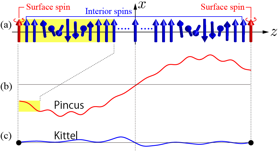
Figure 1: (a) The interior (blue) and surface end (red) spins which form the chiral soliton lattice. (b) The soft boundary condition gives rise to the Pincus mode which is incommensurate with respect to the background system. (c) The perpendicular ac field ${\beta}_{x}(\tau)$ further excites the additional Kittel mode (ripple) which is pinned down at both ends and commensurate with respect to the background system.

Now, we separately treat the dynamics of the interior and end spins. To analyze the dynamics of the interior spins, the term with $\boldsymbol{H}_{s}$ can be discarded. Long period modulation of the magnetic structure makes it legitimate to take a continuum limit of the lattice Hamiltonian (1),

$$\mathcal{H}_{\text{interior}} =\frac{JS^{2}}{2}\left(\partial_{z}\theta\right)^{2}+\frac{JS^{2}}{2}\sin^{2}\theta\left(\partial_{z}\varphi\right)^{2}$$

$$-DS^{2}\sin^{2}\theta\partial_{z}\varphi$$

$$-\left[H_{0}+h_{x}(t)\right]S\sin\theta\cos\varphi-h_{z}(t)S\cos\theta.$$ (2)

Here, $\varphi$ and $\theta$ are the angles that the magnetization, $\boldsymbol{S}(\mathbf{r})=S\left(\sin\theta\cos\varphi,\sin\theta\sin\varphi,\cos\theta\right)$, makes with respect to the $x$ and $z$ axis, respectively, with the film lying parallel to the $xz$ plane. The field $\boldsymbol{H}_{0}$ is directed along the $x$-axis. The presence of the field alters a helical spin arrangement of the ground state to the chiral soliton lattice Dzyaloshinskii1964 ; Book2015 . The classical equations of motion, $\hbar S\sin\theta\partial_{t}\theta=\delta\mathcal{H}_{\text{interior}}/\delta\varphi$ and $\hbar S\sin\theta\partial_{t}\varphi=-\delta\mathcal{H}_{\text{interior}}/\delta\theta$, can be easily shown to be

$$\partial_{\tau}\theta =-\sin\theta\partial_{z}^{2}\varphi-2\cos\theta\partial_{z}\theta\partial_{z}\varphi$$

$$+2\left(D/J\right)\cos\theta\partial_{z}\theta+\left[\beta_{0}+\beta_{x}(t)\right]\sin\varphi,$$ (3)

$$-\sin\theta\partial_{\tau}\varphi =\sin\theta\cos\theta\left(\partial_{z}\varphi\right)^{2}-\partial_{z}^{2}\theta$$

$$-2\left(D/J\right)\sin\theta\cos\theta\partial_{z}\varphi$$

$$-\left[\beta_{0}+\beta_{x}(t)\right]\cos\theta\cos\varphi+\beta_{z}(t)\sin\theta,$$ (4)

where $\tau=JSt/\hbar$, $\beta_{0}=H_{0}/JS$ and $\beta_{x,z}(t)=h_{x,z}(t)/JS$. We note that the frequency scale is $JS/h\sim 5.6\times 10^{11}$Hz (by choosing $J=18$KShinozaki2016 and $S=3/2$).

The ground state is specified by $\theta_{0}=\pi/2$ and

$$\varphi_{0}(z)=\phi_{0}-2\text{am}\left(\frac{\sqrt{\beta_{0}}}{\kappa}z+\phi_{1}\right).$$ (5)

Here, $\mathrm{am}\text{ }$is the Jacobi amplitude function. The elliptic modulus $\kappa$ and two constants,$\ \phi_{0}$($0$ or $\pi$) and $\phi_{1}$($0$ or $K$) are chosen through fitting with the numerical data (see Sec. III). The spatial period of the CSL is $L_{\text{CSL}}=2\kappa K/\sqrt{\beta_{0}}$ and the total number of the solitons is $n=L/L_{\text{CSL}}$. Here, $K$ is the elliptic integral of the first kind.

To consider small dynamical fluctuations around the equilibrium configuration of the CSL, we introduce the $\psi\left(z,t\right)$ (out-of-plane) and $\chi\left(z,t\right)$ (in-plane) fluctuations of the local spins,

$$\left\{\begin{array}[c]{c}\theta(z,\tau)=\dfrac{\pi}{2}+\psi(z,\tau),\\ \varphi(z,\tau)=\varphi_{0}(z)+\chi(z,\tau),\end{array}\right.$$ (6)

where $\left|\psi\right|,\left|\chi\right|\ll 1$. Then, linear approximation of Eqs.(3) and (4) leads to (see Appendix A)

$$\frac{\kappa^{2}}{\beta_{0}}\frac{\partial\psi\left(z,t\right)}{\partial\tau} =\hat{\mathcal{L}}_{\varphi}\chi\left(z,t\right)+\frac{\kappa^{2}}{\beta_{0}}{\beta}_{x}(\tau)\sin\varphi_{0}\left(z\right),$$ (7)

$$\frac{\kappa^{2}}{\beta_{0}}\frac{\partial\chi\left(z,t\right)}{\partial\tau} =-\hat{\mathcal{L}}_{\theta}\psi\left(z,t\right)-\frac{\kappa^{2}}{\beta_{0}}{\beta}_{z}(\tau),$$ (8)

where $\hat{\mathcal{L}}_{\varphi}=-\partial_{\bar{z}}^{2}+2\kappa^{2}\text{sn}^{2}\bar{z}-\kappa^{2}$ and $\hat{\mathcal{L}}_{\theta}=-\partial_{\bar{z}}^{2}+2\kappa^{2}\text{sn}^{2}\bar{z}+4-3\kappa^{2}$ are the linear Lamé operators, and $\bar{z}=z\sqrt{\beta_{0}}/\kappa$ with sn being the Jacobi sn function.

We here comment on the structure of the EOMs. $\hat{\mathcal{L}}_{\varphi}$ and $\hat{\mathcal{L}}_{\theta}$ give the propagating  wave described by the eigenfunctions of the Lamé equation. The propagating solution gives the spin resonance in an infinite system.Kishine2009 In the present case, the soft boundary condition gives rise to standing waves, where the end surface spins softly fluctuate. We call this mode ‘Pincus mode’ [see Fig. 1(b)] which is incommensurate with respect to the background system.

Next, the dynamics of the surface spins is described by (see Appendix B for details)

$$\frac{\partial\psi_{s}}{\partial\tau} =\pm\partial_{z}\chi_{s}-\frac{1}{2}\partial_{z}^{2}\chi_{s}\mp(D/J)\partial_{z}\varphi_{0}\partial_{z}\chi_{s}$$

$$+{\beta}_{x}(\tau)\sin\varphi_{0}+\left(\beta_{\text{s}}+\beta_{0}\right)\cos\varphi_{0}\cdot\chi_{s},$$ (9)

$$\frac{\partial\chi_{s}}{\partial\tau} =\mp\partial_{z}\psi_{s}+\frac{1}{2}\partial_{z}^{2}\psi_{s}+\frac{1}{2}\left(\partial_{z}\varphi_{0}\right)^{2}\psi_{s}$$

$$+(D/J)\left(\partial_{z}\varphi_{0}\right)\psi_{s}-\frac{1}{2}(D/J)\left(\partial_{z}^{2}\varphi_{0}\right)\psi_{s}$$

$$-\left[\left(\beta_{\text{s}}+\beta_{0}\right)\cos\varphi_{0}\right]\psi_{s},$$ (10)

where $\beta_{\text{s}}=H_{\text{s}}/JS$ is the pinning field strength. The upper (lower) sign refers to the end spins at the right (left) end site, $z=L/2$ or $-L/2$, that indexed by $s=$r or l, respectively.

The precession of the surface spins with the frequency, $\Omega_{\text{surface}}$, are eventually caught up in the interior spin wave with the frequency, $\Omega_{\text{interior}}$. Then, the matching condition $\Omega_{\text{surface}}=\Omega_{\text{interior}}$, which is called the Davis-Puszkarski equation,Davis1963 ; Puszkarski1973 ; Banavar1978 determines the overall spin wave dispersion. The SSW modes are quite sensitive to the direction of the external magnetic $\boldsymbol{h}(t)$, i.e., whether $\boldsymbol{h}(t)$ is paralell to the chiral axis [$\boldsymbol{h}(t)=h_{0z}\hat{\mathbf{e}}_{z}$] or perpendicular to the chiral axis [$\boldsymbol{h}(t)=h_{0x}\hat{\mathbf{e}}_{x}$].

Before presenting the detailed analysis, we give an intuitive argument on this effect. In Eq. (7), the term including ${\beta}_{x}(\tau)\sin\varphi_{0}\left(z\right)$ plays a role of space-time dependent external force whose ‘spatial frequency’ is equal to the spatial period of the CSL, $L_{\text{CSL}}$. Therefore, when ${\beta}_{x}(\tau)$ is present, there appears a series of the additional standing spin waves with their basis spanned by the eigenfunctions of the Lamé equation. This additional modes are completely pinned down at the both ends $z=\pm L/2$. We call this mode ‘Kittel ripple’ [see Fig. 1(c)], which appears only for finite ${\beta}_{x}(\tau)$ and commensurate to the background system. Unlike the case of ${\beta}_{x}(\tau)$, the term including ${\beta}_{z}(\tau)$ in Eq. (8) is spatially uniform and can excite the Pincus mode only. As we will discuss in more detail below, the presence or absences of the Kittel ripple may provide an explanation for the experimentally found difference in the SSW modes depending on the direction of the ac field.Goncalves2017

III Numerical simulations

III.1 Simulation scheme

To gain insight into the resonant dynamics, we first perform numerical simulations similar to those used to study coherent sliding dynamics driven by crossed magnetic fields in the mono-axial chiral helimagnet Kishine2012 . The numerical analysis is based on the lattice version of Eqs. (3,4) for the interior spins

$$\frac{\partial\theta_{i}}{\partial\tau} =\sqrt{1+\left(D/J\right)^{2}}\sin\theta_{i-1}\sin\left(\varphi_{i}-\varphi_{i-1}-\delta\right)$$

$$-\sqrt{1+\left(D/J\right)^{2}}\sin\theta_{i+1}\sin\left(\varphi_{i+1}-\varphi_{i}-\delta\right)$$

$$+\left(\beta_{0}+\beta_{x}\right)\sin\varphi_{i},$$ (11)

$$\frac{\partial\varphi_{i}}{\partial\tau} =-\left(\cos\theta_{i+1}+\cos\theta_{i-1}\right)$$

$$+\sqrt{1+\left(D/J\right)^{2}}\text{cot}\theta_{i}\sin\theta_{i-1}\cos\left(\varphi_{i}-\varphi_{i-1}-\delta\right)$$

$$+\sqrt{1+\left(D/J\right)^{2}}\text{cot}\theta_{i}\sin\theta_{i+1}\cos\left(\varphi_{i+1}-\varphi_{i}-\delta\right)$$

$$+\left(\beta_{0}+\beta_{x}\right)\text{cot}\theta_{i}\cos\varphi_{i}-\beta_{z},$$ (12)

where $\delta=\text{arctan}(D/J)$, and complemented by equations for the boundaries (75) and (76). For the boundary spins, $\beta_{x}$ is substituted for $\beta_{\text{s}}$. The length of the system is chosen $L=411$ which corresponds to the number of kinks accommodated inside the system, $n_{\text{max}}=[Lq_{s}/2\pi]=10$. The value is about the same order of magnitude as the number of kinks confined within grains of a definite crystalline chirality in thin films of CrNb₃S₆,Togawa2012 where the pitch of the helix is $q_{s}=0.16$.

A search for a static configuration of the ground state is described in detail in Ref. Kishine2012 . The static solution found with the aid of the relaxation method serves as an initial condition for the dynamical equations addressed by the eight-order Dormand-Prince method with an adaptive step-size control. To search for a resonant frequency the following procedure is adopted. Time evolution of $\varphi_{i}(\tau)$, $\theta_{i}(\tau)$ is determined as a response to the ac-field $\beta_{\alpha}(\tau)=\beta_{\alpha 0}\left[1-\exp(-\tau)\right]$ ($\alpha=x,z$) at the start. The Fourier transform of the ac-field signal is distributed over a continuous frequency range that enable to localize an approximate position of an intrinsic resonance. To get its precise value, the spin dynamics equations are again integrated but now the ac-field is periodical, $\beta_{\alpha}(\tau)=\beta_{\alpha 0}\sin\left(\Omega\tau\right)$, where $\alpha=x$ or $z$. Provided that the frequency $\Omega$ lies near the resonance, this gives rise to characteristic beatings. Re-examination of these signals by Fourier analysis specifies an exact position of the resonance frequency.

Here, we separately discuss results of numerical solution for configurations examined experimentally in Ref. Goncalves2017 : when (I) the ac microwave field is applied parallel to the chiral axis, and when (II) the ac-field is applied perpendicular to the axis.

III.2 Case I: the ac magnetic field is parallel to the chiral axis

In the case I, we expect the driving ac-field excites the Pincus modes which are symmetric with respect to reflection across the center ($z=0$), because the pinning fields $\beta_{\text{s}}(t)$ act on both ends in a symmetric manner.

In Fig. 2, we show the spatial profiles of $\varphi$ and $\theta$ associated with the standing waves over the helical structure under zero dc magnetic field ($\beta_{0}=0$). The parameters are taken as $\beta_{\text{s}}=0.02$ and $\beta_{z0}=0.0001$. The SSW of the first and third orders occur at the frequencies $\Omega=0.0011$ and $\Omega=0.0030$, respectively. As evident from Fig. 2, there arise the SSWs with the number of half wavelengths being approximately odd in a similar way to those in the original Kittel’s theory.Kittel1958 It should be noted that the amplitude of the $\varphi$-oscillations is ten times the $\theta$-mode amplitude. These findings fit into the idea that spin-wave modes in a thin film behave like a vibration of a rope clamped at the both ends, when some anisotropy field essentially or partially pins down boundary spins.

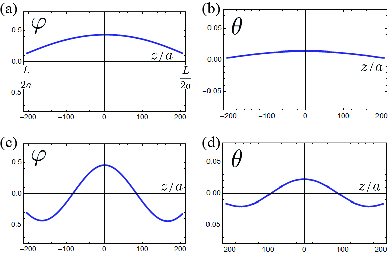
Figure 2: The spatial profiles of $\varphi$ and $\theta$ associated with the standing waves over the helical structure under zero dc magnetic field ($\beta_{0}=0$). The ac field is applied parallel to the chiral axis. The SSW of the first order at the frequency $\Omega=0.0011$ (a,b) and of the third order at the frequency $\Omega=0.0030$ (c,d). The parameters are taken as $\beta_{\text{s}}=0.02$ and $\beta_{z0}=0.0001$ .

In Fig. 3, we show the spatial profiles of $\varphi$ and $\theta$ associated with the standing waves over the CSL structure under finite dc magnetic field ($\beta_{0}=0.002$). The parameters are taken as $\beta_{\text{s}}=0.02$ and $\beta_{x0}=0.0001$. The SSW of the first and third orders occur at the frequencies $\Omega=0.00105$ and $\Omega=0.00305$, respectively. Just as in the case of Fig. 2, one may immediately recognize the symmetric modes with zero and two nodes, but the profiles of these excitations look different. It is clear that some short-scale oscillations, seen as a ripple over the standing wave background, contribute to the signal. We will discuss the origin of this ripple in Sec. IV.

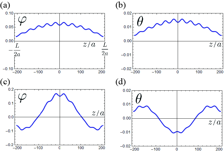
Figure 3: The spatial profiles of $\varphi$ and $\theta$ associated with the standing waves over the CSL structure under finite dc magnetic field ($\beta_{0}=0.002$). The ac field is applied parallel to the chiral axis. The SSW of the first order at the frequency $\Omega=0.00105$ (a,b), and of the third order at the frequency $\Omega=0.00305$ (c,d). The parameters are taken as $\beta_{\text{s}}=0.02$ and $\beta_{x0}=0.0001$.

III.3 Case II: the ac magnetic field is perpendicular to the chiral axis

Next we consider the case II. In this case, we expect the driving ac-field excites the Pincus modes which are antisymmetric with respect to reflection across the center ($z=0$), because in Eq. (7) the space-dependent field $\sin\varphi_{0}\left(z\right)$ is an odd function of $z$.

In Fig. 4, we show the spatial profiles of $\varphi$ and $\theta$ associated with the standing waves over the helical structure under a zero dc magnetic field ($\beta_{0}=0$). The parameters are taken as $\beta_{\text{s}}=0.02$ and $\beta_{x0}=0.0001$. The SSW of the second order occurs at the frequencies $\Omega=0.0021$. As compared with the case I, shown in Fig. 2, we recognize that the additional ripples with tiny amplitude are superimposed on the background Pincus mode. This additional ripples are caused by the space-time dependent external force, ${\beta}_{x}(\tau)\sin\varphi_{0}\left(z\right)$. Because the term $\sin\varphi_{0}\left(z\right)$ vanishes at both ends $z=\pm L/2$, the additional modes are analogous to the original Kittel modesKittel1958 which are completely pinned down at both ends.

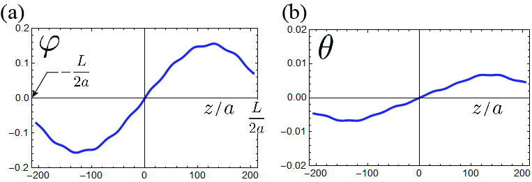
Figure 4: The spatial profiles of (a) $\varphi$ and (b) $\theta$ associated with the second order standing waves over the helical structure under zero dc magnetic field ($\beta_{0}=0$). The ac field is applied perpendicular to the chiral axis at the frequency $\Omega=0.0021$.

In Fig. 5, we show the spatial profiles of $\varphi$ and $\theta$ associated with the standing waves over the CSL structure under a finite dc magnetic field ($\beta_{0}=0.002$). The parameters are taken as $\beta_{\text{s}}=0.02$ and $\beta_{x0}=0.0001$. The SSW of the second order occurs at the frequencies $\Omega=0.0022$. As with the case shown in Fig. 4, the additional Kittel ripples are superimposed on the background Pincus mode, although it is almost invisible because of tiny amplitudes.

Figure 5: The spatial profiles of (a) $\varphi$ and (b) $\theta$ associated with the second order standing waves over the CSL structure under finite dc magnetic field ($\beta_{0}=0.002$). The ac field is applied parallel to the chiral axis at the frequency $\Omega=0.0022$.

Based on the numerical findings presented above, it is evident that the SSW modes are significantly affected by the movable boundaries which causes Pincus modes. Furthermore, when the ac field is applied perpendicular to the chiral axis (case II), the additional Kittel ripples are superimposed. Our next challenge is to elaborate an appropriate analytical theory of the dynamics.

IV Analytical theory of the SSW dynamics

In this section, we present an analytical theory in details. We consider the following four cases depending on ‘case I or II’ and ‘the SSW over either CSL or helical structure.’ Throughout this section, we follow the technical scheme for the Davis-Puszkarski equation which is summarized in Appendix C from general viewpoints.

IV.1 Case I: the ac magnetic field is parallel to the chiral axis

IV.1.1 SSW over the CSL

In the case I, the interior spins are subject to the uniform ac-field only. In Eqs. (7) and (8), ${\beta}_{x}(\tau)=0$ and only the spatially uniform field, ${\beta}_{z}(\tau)$, excites the intrinsic SSW modes. So, we can also drop ${\beta}_{z}(\tau)$ for the purpose of obtaining the SSW dispersion. Then, the coupled equations are solved by separation of variables, $\chi(z,\tau)=\nu(\bar{z})Z(\tau)$ and $\psi(z,\tau)=\nu(\bar{z})\xi(\tau)$. Both $\chi$ and $\psi$ fields share the same spatial parts $\nu(\bar{z})$ which is the eigenfunction of the Lamé equation,Book2015 and satisfy

$$\hat{\mathcal{L}}_{\varphi}\nu_{q}(\bar{z}) =\lambda^{(\varphi)}\nu_{q}(\bar{z})$$

$$={\kappa}^{\prime 2}\text{sn}^{2}(\alpha,\kappa^{\prime})\nu_{q}(\bar{z}),$$ (13)

$$\hat{\mathcal{L}}_{\theta}\nu_{q}(\bar{z}) =\lambda^{(\theta)}\nu_{q}(\bar{z})$$

$$=\left[{\kappa}^{\prime 2}\text{sn}^{2}(\alpha,\kappa^{\prime})+2+2{\kappa}^{\prime 2}\right]\nu_{q}(\bar{z}).$$ (14)

Here, the real parameter $\alpha$ lies in the range $-K^{\prime}<\alpha<K^{\prime}$, where $K^{\prime}$ is the elliptic integral of the first kind with the complementary elliptic modulus, ${\kappa}^{\prime 2}=1-{\kappa}^{2}$. The lower index of the eigenfunctions stands for the wave number of the Bloch wave,

$$q(\alpha)=\frac{\sqrt{\beta_{0}}}{\kappa}\left[Z(\alpha,{\kappa}^{\prime})+\frac{\pi\alpha}{2KK^{{}^{\prime}}}\right],$$ (15)

which is related with the eigenvalues $\lambda^{(\varphi,\theta)}$ through an implicit parameter $\alpha$. $Z(\alpha,{\kappa}^{\prime})$ represents Jacobi’s zeta-function. The allowed values of $q(\alpha)$ are to be determined by this equation.

The temporal parts $Z(\tau)$ and $\xi(\tau)$ are nothing but the collective coordinates associate with $\varphi$ and $\theta$ fields, respectively, and describe the collective dynamics of the CSL as a whole. Then, Eqs. (7) and (8), become

$$\left\{\begin{array}[c]{c}\dot{\xi}(\tau)=C_{1}\left(\frac{\beta_{0}}{\kappa^{2}}\right)Z(\tau),\\ \dot{Z}(\tau)=-C_{2}\left(\frac{\beta_{0}}{\kappa^{2}}\right)\xi(\tau),\end{array}\right.$$ (16)

and we immediately have the eigenfrequency $\Omega_{0}=(\beta_{0}/\kappa^{2})\sqrt{C_{1}C_{2}}$ that contains the arbitrary constants $C_{1,2}$ which characterize the separation of variables [$\left(\kappa^{2}/\beta_{0}\right)[Z(\tau)]^{-1}\partial\xi(\tau)/\partial\tau=[\nu(\bar{z})]^{-1}\hat{\mathcal{L}}_{\varphi}\nu(\bar{z})=C_{1}$, for example].

Using (13) and (14), we have $C_{1}C_{2}=\lambda^{(\varphi)}\lambda^{(\theta)}$ which gives rise to the resonance frequency for the interior SSW,

$$\Omega_{\text{interior}}^{2}\left(q\right)=\frac{\beta_{0}^{2}}{\kappa^{4}}{\kappa}^{\prime 2}\text{sn}^{2}(\alpha,\kappa^{{}^{\prime}})\left[{\kappa}^{\prime 2}\text{sn}^{2}(\alpha,\kappa^{{}^{\prime}})+2+2{\kappa}^{\prime 2}\right].$$ (17)

Then, we use the symmetrical solution of the Lamé equation,Book2015

$${\nu_{q}}(\bar{z})\propto\Re\left[\frac{\theta_{4}\left(\frac{\pi}{2K}[\bar{z}-i\alpha-K]\right)}{\theta_{4}\left(\frac{\pi\bar{z}}{2K}\right)}e^{-i\bar{q}\bar{z}}\right],$$ (18)

where $\bar{z}=\sqrt{\beta_{0}}/\kappa(z-L/2)+K$ and $\theta_{4}$ is the Jacobi theta function.

Next, we solve equations of motion for the end surface spins, Eqs.(9) and (10), by means of separation of variables, $\chi_{r,l}(z,\tau)={\nu_{q}}(z)Z_{\text{s}}(\tau)$, $\psi_{r,l}(z,\tau)={\nu_{q}}(z)\xi_{\text{s}}(\tau)$. Here, $\bar{q}=(\kappa/\sqrt{\beta_{0}})q(\alpha)$. It is to be noted that the spatial part ${\nu_{q}}(z)$ is the same as that for the interior spins. This trick, used throughout this paper, provides the resonance frequency for the end surface spins,

$$\begin{array}[c]{c}\Omega_{\text{surface}}^{2}=\dfrac{1}{\nu_{q}^{2}(\bar{z}_{L/2})}\Biggl{[}\dfrac{\sqrt{\beta_{0}}}{\kappa}\nu_{q}^{{}^{\prime}}(\bar{z}_{L/2})-\dfrac{\beta_{0}}{2\kappa^{2}}\nu_{q}^{{}^{\prime\prime}}(\bar{z}_{L/2})\Biggr{.}\\ -\dfrac{D}{J}\dfrac{\beta_{0}}{\kappa^{2}}\varphi_{0}^{{}^{\prime}}(\bar{z}_{L/2})\nu_{q}^{{}^{\prime}}(\bar{z}_{L/2})\\ \Biggl{.}+\left(\beta_{0}+\beta_{s}\right)\cos\varphi_{0}(\bar{z}_{L/2})\nu_{q}(\bar{z}_{L/2})\Biggr{]}\\ \times\Biggl{[}\dfrac{\sqrt{\beta_{0}}}{\kappa}\nu_{q}^{{}^{\prime}}(\bar{z}_{L/2})-\dfrac{\beta_{0}}{2\kappa^{2}}\nu_{q}^{{}^{\prime\prime}}(\bar{z}_{L/2})\Biggr{.}\\ -\dfrac{\beta_{0}}{2\kappa^{2}}\nu_{q}(\bar{z}_{L/2})\left(\varphi_{0}^{{}^{\prime}}\right)^{2}(\bar{z}_{L/2})\\ -\dfrac{D}{J}\left\{\dfrac{\sqrt{\beta_{0}}}{\kappa}\varphi_{0}^{{}^{\prime}}(\bar{z}_{L/2})-\dfrac{\beta_{0}}{2\kappa^{2}}\varphi_{0}^{{}^{\prime\prime}}(\bar{z}_{L/2})\right\}\nu_{q}(\bar{z}_{L/2})\\ \Biggl{.}+\left(\beta_{0}+\beta_{\text{s}}\right)\cos\varphi_{0}(\bar{z}_{L/2})\nu_{q}(\bar{z}_{L/2})\Biggr{]}.\end{array}$$ (19)

Now, the matching condition (the Davis-Puszkarski equation)

$$\Omega_{\text{interior}}\left(q\right)=\Omega_{\text{surface}}$$ (20)

leads to the determination of the parameter $\alpha$, and then gives the allowed wavenumber $q$. This algorithm is similar to the case for ferromagnetic thin films Davis1963 ; Puszkarski1973 ; Banavar1978 .

The SSW is obtained by superposition of two waves propagating into the opposite directions,

$$\chi(\bar{z},\tau)=\frac{{\nu_{q}}(\bar{z}_{L/2+z})+{\nu_{q}}(\bar{z}_{L/2-z})}{{\nu_{q}}(\bar{z}_{L})+{\nu_{q}}(\bar{z}_{0})}\chi(\bar{z}_{L/2},\tau).$$ (21)

We obtain a similar expression for $\psi(\bar{z},\tau)$. Here, the boundary functions are taken from the numerical data. In Fig. 6, we show comparison between numerical and analytical results for the spatial profiles of $\varphi$ and (b) $\theta$ associated with the first order standing waves over the CSL structure under finite dc magnetic field ($\beta_{0}=0.002$). It is seen that the analytical results are consistent with the numerical ones.

Figure 6: Comparison between numerical (red line) and analytical (blue line) results for the spatial profiles of (a) $\varphi$ and (b) $\theta$ associated with the first order standing waves over the CSL structure under finite dc magnetic field ($\beta_{0}=0.002$). The parameters are taken as $\beta_{\text{s}}=0.02$ and $\beta_{x0}=0.0001$. Analytical result is obtained by Eqs. (21) at $\tau=5600$.

Analytical results enable us to understand the origin of the ripples. For this purpose, we decompose Eq. (18) into ‘Bloch wave’ ($e^{-i\bar{q}\bar{z}}$) and ‘Lamé ripple’ [ ${\theta_{4}\left(\frac{\pi}{2K}[\bar{z}-i\alpha-K]\right)}/{\theta_{4}\left(\frac{\pi\bar{z}}{2K}\right)}$]. We separately show the spatial profiles of these waves in Fig. 7. It is seen that the Bloch part behaves like a smooth background, while the Lamé part exhibits the short-wavelength modulation (ripple) which directly reflects the spatial period of the CSL, $L_{\text{CSL}}$.

Figure 7: Schematic demonstration of how the SSW wave function over the CSL, Eq. (18), is decomposed into (a) Bloch wave ($e^{-i\bar{q}\bar{z}}$) and (b) Lamé ripple [ ${\theta_{4}\left(\frac{\pi}{2K}[\bar{z}-i\alpha-K]\right)}/{\theta_{4}\left(\frac{\pi\bar{z}}{2K}\right)}$]. The parameter setting is the same as in the case of Fig. 6.

In Fig. 8, the spectrum of the SSW of the first, second and third orders, where both numerical and analytical results are shown for comparison. It is evident that the theoretical and numerical results are in good agreement.

Figure 8: (a) Schematic view of the case I configuration. (b) Resonance frequency $\Omega_{0}$ for standing waves of the first order ($\Circle$ - numerical data, $\CIRCLE$ - theory), the second order ($\Box$ - numerical data, $\blacksquare$ - theory) and the third order ($\vartriangle$ - numerical data, $\blacktriangle$ - theory) depending on the transverse dc-field $\beta_{0}$.

IV.1.2 SSW over the simple helix

We here separately discuss the case of zero magnetic dc-field ($\beta_{0}=0$). In this case, the ground state is a simple helix with an uniform modulation and the above analysis can be repeated in much simpler manner.

The helical structure of the interior spins is described by $\theta_{0}=\pi/2$ and $\varphi_{0}=q_{s}(z-z_{0})$. The helical pitch is determined through an equation (see Appendix B for derivation)

$$0=\sin q_{s}-\left(D/J\right)\cos q_{s}\mp\beta_{\text{s}}\sin\varphi\left(\mp L/2\right).$$ (22)

The presence of the pinning field complicate the condition for $q_{s}$.

The equations of motion (7) and (8) may be recast in the form

$$\partial_{\tau}\psi =-\partial_{z}^{2}\chi,$$ (23)

$$\partial_{\tau}\chi =\left[\partial_{z}^{2}-2({D}/{J})q_{s}+q_{s}^{2}\right]\psi-\beta_{z}(\tau).$$ (24)

We look for solutions in the form of the standing wave, $\cos(kz)$, with the wavevector $k$. The resonance frequency for the interior spins is then given by

$$\Omega_{\text{interior}}^{2}=k^{2}\left[k^{2}-q_{s}^{2}+2q_{s}({D}/{J})\right].$$ (25)

On the other hand, the resonance frequency for the surface end spins is obtained to be

$$\Omega_{\text{surface}}^{2} =\left[k\tan\left(k{L/2}\right)\left\{1+(D/J)q_{s}\right\}\right.$$

$$\left.-k^{2}/2-\beta_{\text{s}}\cos\varphi_{0}\left({L/2}\right)\right]$$

$$\times\left\{k\tan\left(k{L/2}\right)-k^{2}/2+q_{s}^{2}/2\right.$$

$$\left.-(D/J)q_{s}-\beta_{\text{s}}\cos\varphi_{0}\left({L/2}\right)\right\}.$$ (26)

Then, the Davis-Puszkarski equation leads to the determination of allowed values of $k$.

By performing numerical estimations for $D/J=0.16$, $\beta_{\text{s}}=0.02$, $\varphi_{0}(\mp L/2)=\pm 31.6369$, where $L/2=205$, we obtain $k^{(1)}=0.006671$, $\Omega_{0}^{(1)}=0.001067$ and $k^{(3)}=0.020279$, $\Omega_{0}^{(3)}=0.003268$ for the standing waves of the 1st and 3rd orders, respectivelyTermin . This result is included in Fig. 8.

IV.2 Case II: the ac magnetic field is perpendicular to the chiral axis

IV.2.1 SSW over the CSL

Now we examine the most complicated case, where the SSW is excited over the CSL by the ac-field applied perpendicular to the chiral axis. An essential feature of this case lies in the fact that the interior spins experience space-time dependent Zeeman interaction with an effective field $\beta_{\text{eff}}(z,\tau)=\sin\varphi_{0}(z){\beta}_{x}(\tau)$ in Eqs. (7). This term prevents us to apply separation of variables. To attack the problem the method of transformations leading to homogeneous boundary conditions may be used Polyanin2002 . For the purpose, we solve initially the EOM for the interior spins, by assuming that dynamics of the end spins is known. The results obtained in this fashion are then used to address the problem to describe dynamics of the end surface spins in a self-consistent manner.

To realize the scheme the spin fluctuations may be expanded as

$$\chi(\bar{z},\tau) =\frac{\nu_{q}(\bar{z})}{\nu_{q}(\bar{z}_{L/2})}\chi(\bar{z}_{L/2},\tau)+\epsilon\tilde{\chi}(\bar{z},\tau),$$ (27)

$$\psi(\bar{z},\tau) =\frac{\nu_{q}(\bar{z})}{\nu_{q}(\bar{z}_{L/2})}\psi(\bar{z}_{L/2},\tau)+\epsilon\tilde{\psi}(\bar{z},\tau),$$ (28)

where the first terms correspond to the standing wave antisymmetric with respect to reflection across the center,

$${\nu_{q}}(\bar{z})\propto\Im\left[\frac{\theta_{4}\left(\frac{\pi}{2K}[\bar{z}-i\alpha-K]\right)}{\theta_{4}\left(\frac{\pi\bar{z}}{2K}\right)}e^{-i\bar{q}\bar{z}}\right].$$ (29)

The second terms in the r.h.s. of Eqs. (27) and (28) give rise to the additional short-wavelength ripples with the both ends being completely pinned, i.e., $\tilde{\chi}(\bar{z}_{\pm L/2},\tau)=0$ and $\tilde{\psi}(\bar{z}_{\pm L/2},\tau)=0$. In view of the complete pinning, we call this additional ripple the ‘Kittel ripple.’

The amplitude of the Kittel ripple is proportional to the small parameter $\epsilon$. From the beginning, the dynamics of the end spins, i.e. $\chi(\bar{z}_{L/2},\tau)$ and $\psi(\bar{z}_{L/2},\tau)$, is considered as being known. Due to odd parity of the function $\nu_{q}(\bar{z})$, the oscillations of the boundary spins are anti-synchronized, i.e. $\chi(\bar{z}_{-L/2},\tau)=-\chi(\bar{z}_{L/2},\tau)$ and $\psi(\bar{z}_{-L/2},\tau)=-\psi(\bar{z}_{L/2},\tau)$.

Substituting Eqs. (27) and (28) into Eqs.(7) and (8), we obtain the coupled equations of the zeroth-order in $\epsilon$,

$$\dot{\psi}\left(\bar{z}_{L/2},\tau\right) =\left(\beta_{0}/\kappa^{2}\right)\lambda^{(\varphi)}\chi\left(\bar{z}_{L/2},\tau\right),$$ (30)

$$\dot{\chi}\left(\bar{z}_{L/2},\tau\right) =-\left(\beta_{0}/\kappa^{2}\right)\lambda^{(\theta)}\psi\left(\bar{z}_{L/2},\tau\right),$$ (31)

which gives the resonance frequency for the Pincus mode of the interior spins,

$$\Omega_{\text{interior-Pincus}}^{2}=\frac{\beta_{0}^{2}}{\kappa^{4}}\lambda^{(\varphi)}\lambda^{(\theta)}$$

$$=\frac{\beta_{0}^{2}}{\kappa^{4}}{\kappa}^{\prime 2}\text{sn}^{2}(\alpha,\kappa^{{}^{\prime}})\left[{\kappa}^{\prime 2}\text{sn}^{2}(\alpha,\kappa^{{}^{\prime}})+2+2{\kappa}^{\prime 2}\right],$$ (32)

with no restriction on $\alpha$. We call this ‘interior Pincus’ mode.

The coupled equations of the first-order in $\epsilon$ are found to be

$$\dot{\tilde{\psi}}(\bar{z},t) =\frac{\beta_{0}}{\kappa^{2}}\hat{\mathcal{L}}_{\varphi}\tilde{\chi}(\bar{z},t)+\frac{\beta_{x}(\tau)}{\epsilon}\sin\varphi_{0}(\bar{z}),$$ (33)

$$\dot{\tilde{\chi}}(\bar{z},t) =-\frac{\beta_{0}}{\kappa^{2}}\hat{\mathcal{L}}_{\theta}\tilde{\psi}(\bar{z},t).$$ (34)

The resonance frequency for the Kittel ripples of the interior spins is now

$$\Omega_{\text{interior-Kittel}}^{2}\left(q\right) =\frac{\beta_{0}^{2}}{\kappa^{4}}{\kappa}^{\prime 2}\text{sn}^{2}(\alpha,\kappa^{{}^{\prime}})$$

$$\times\left[{\kappa}^{\prime 2}\text{sn}^{2}(\alpha,\kappa^{{}^{\prime}})+2+2{\kappa}^{\prime 2}\right],$$ (35)

under the restriction on $\alpha$ due to the boundary condition, $\nu_{q}(\bar{z}_{\pm L/2})=0$. We look for solutions of Eqs.(33) and (34) in the form

$$\tilde{\psi}(\bar{z},\tau) =\sum_{n}\tilde{\psi}_{n}(\tau)\nu_{q_{n}}(\bar{z}),$$ (36)

$$\tilde{\chi}(\bar{z},\tau) =\sum_{n}\tilde{\chi}_{n}(\tau)\nu_{q_{n}}(\bar{z}),$$ (37)

where the wavevectors $q_{n}$ are determined by $\nu_{q_{n}}(\bar{z}_{\pm L/2})=0$.

Inserting Eqs. (36) and (37) into Eqs. (33) and (34) yields

$$\tilde{\chi}_{n}(\tau) =f_{n}\frac{\beta_{x0}}{\epsilon}\frac{\kappa^{2}}{\beta_{0}}\frac{\Omega_{n}}{\lambda_{n}^{(\varphi)}}\frac{\left[\Omega_{n}\sin(\Omega\tau)-\Omega\sin(\Omega_{n}\tau)\right]}{\Omega^{2}-\Omega_{n}^{2}},$$ (38)

$$\tilde{\psi}_{n}(\tau) =f_{n}\frac{\beta_{x0}}{\epsilon}\Omega\frac{\left[\cos(\Omega_{n}\tau)-\cos(\Omega\tau)\right]}{\Omega^{2}-\Omega_{n}^{2}},$$ (39)

where $\Omega_{n}$ is given by (35) being estimated for the $q_{n}$, and

$$f_{n}=\frac{\int_{-\bar{z}_{L/2}}^{\bar{z}_{L/2}}\sin\varphi_{0}(\bar{z})\nu_{q_{n}}(\bar{z})d\bar{z}}{\int_{-\bar{z}_{L/2}}^{\bar{z}_{L/2}}\nu_{q_{n}}^{2}(\bar{z})d\bar{z}}.$$ (40)

The function $\sin\varphi_{0}$ is antisymmetric with respect to reflection across the center of the system, and therefore the summation in (36) and (37) should include the odd functions $\nu_{q_{n}}(\bar{z})$ only.

In Fig. 9, we show comparison between numerical and analytical results for the spatial profiles of $\varphi$ and $\theta$ associated with the second order standing waves over the CSL structure under finite dc magnetic field.

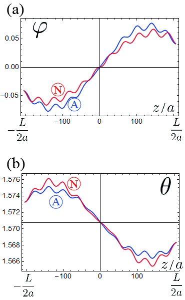
Figure 9: Comparison between numerical (red line) and analytical (blue line) results for the spatial profiles of (a) $\varphi$ and (b) $\theta$ associated with the second order standing waves over the CSL structure under finite dc magnetic field ($\beta_{0}=0.002$). The parameters are taken as $\beta_{s}=0.02$ and $\beta_{x0}=0.0001$. Analytical result is obtained by Eqs. (27) and (28) with $\epsilon=2/3$ at $\tau=6000$.

We now consider the boundary values $\chi(\bar{z}_{L/2},\tau)$ and $\psi(\bar{z}_{L/2},\tau)$. To make this in a self-consistent manner, we neglect the additional Kittel ripple terms in Eqs.(27) and (28), which become vanishingly small in the vicinity of the boundaries,

$$\chi(\bar{z},\tau) \sim c_{\chi}\frac{\nu_{q}(\bar{z})}{\nu_{q}(\bar{z}_{L/2})}\chi(\bar{z}_{L/2},\tau),$$ (41)

$$\psi(\bar{z},\tau) \sim c_{\psi}\frac{\nu_{q}(\bar{z})}{\nu_{q}(\bar{z}_{L/2})}\psi(\bar{z}_{L/2},\tau),$$ (42)

where $c_{\chi}$ and $c_{\psi}$ are some constants.

Substitution of (41) and (42) into Eqs.(9) and (10) leads to the differential equations for the two unknowns $\psi\left(z_{L/2},\tau\right)$ and $\chi\left(z_{L/2},\tau\right)$

$$\dot{\psi}\left(z_{L/2},\tau\right) =-\frac{c_{\chi}}{c_{\psi}}A_{q}\chi\left(z_{L/2},\tau\right)+\frac{{\beta}_{x}(\tau)}{c_{\psi}}\sin\varphi_{0}(z_{L/2}),$$ (43)

$$\dot{\chi}\left(z_{L/2},\tau\right) =\frac{c_{\psi}}{c_{\chi}}B_{q}\psi\left(z_{L/2},\tau\right),$$ (44)

where

$$A_{q} =-\frac{\nu_{q}^{{}^{\prime}}(z_{L/2})}{\nu_{q}(z_{L/2})}+\frac{1}{2}\frac{\nu_{q}^{{}^{\prime\prime}}(z_{L/2})}{\nu_{q}(z_{L/2})}+\frac{D}{J}\frac{\nu_{q}^{{}^{\prime}}(z_{L/2})}{\nu_{q}(z_{L/2})}\varphi_{0}^{{}^{\prime}}(z_{L/2})$$

$$-\left(\beta_{\text{s}}+\beta_{0}\right)\cos\varphi_{0}(z_{L/2}),$$ (45)

$$B_{q} =-\frac{\nu_{q}^{{}^{\prime}}(z_{L/2})}{\nu_{q}(z_{L/2})}+\frac{1}{2}\frac{\nu_{q}^{{}^{\prime\prime}}(z_{L/2})}{\nu_{q}(z_{L/2})}+\frac{1}{2}{\varphi^{{}^{\prime}}}_{0}^{2}(z_{L/2})$$

$$+\frac{D}{J}\varphi_{0}^{{}^{\prime}}(z_{L/2})-\frac{D}{2J}\varphi_{0}^{{}^{\prime\prime}}(z_{L/2})$$

$$-\left(\beta_{\text{s}}+\beta_{0}\right)\cos\varphi_{0}(z_{L/2}).$$ (46)

Then, the resonance frequency for the end surface spins is

$$\Omega_{\text{surface-Pincus}}=\sqrt{A_{q}B_{q}},$$ (47)

which is identified with as ‘surface Pincus’ mode. Choosing the initial values $\psi\left(z_{L/2},0\right)=0$ and $\chi\left(z_{L/2},0\right)=0$ that is consistent with the field ${\beta}_{x}(\tau)=\beta_{x0}\sin\left(\Omega\tau\right)$, we find

$$\chi\left(z_{L/2},\tau\right) =\frac{\beta_{x0}B_{q}}{c_{\chi}}\frac{\sin\varphi_{0}(z_{L/2})}{\Omega_{0}\left(\Omega_{0}^{2}-\Omega^{2}\right)}\left[\Omega_{0}\sin\left(\Omega\tau\right)-\Omega\sin\left(\Omega_{0}\tau\right)\right],$$ (48)

$$\psi\left(z_{L/2},\tau\right) =\frac{\beta_{x0}}{c_{\psi}}\frac{\Omega\sin\varphi_{0}(z_{L/2})}{\Omega^{2}-\Omega_{0}^{2}}\left[\cos\left(\Omega_{0}\tau\right)-\cos\left(\Omega\tau\right)\right],$$ (49)

where $\Omega_{0}=\Omega_{\text{surface-Pincus}}=\Omega_{\text{interior-Pincus}}$. This matching condition leads to the determination of the wavenumber $q$.

Analytical results obtained here enable us to understand how the SSWs are constructed from the Bloch waves, Lame ripples and the Kittel ripples. In Fig. 10, we separately show the spatial profile of $\chi(\bar{z}_{L/2},\tau)$ and $\epsilon\tilde{\chi}(\bar{z},\tau)$ in Eq. (27). The Pincus modes consist of the slowly-varying Bloch wave and short-wavelength Lamè ripple. On the other hand, Kittel ripple is completely pinned down at both ends and has a tiny amplitude.

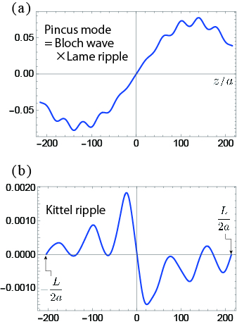
Figure 10: Decomposition of Eq. (27) into the (a) Pincus mode (which is further decomposed into the Bloch wave and Lame ripple, as shown in Fig. 7) and (b) Kittel ripples.

To make supplementary comparison between numerical and analytical results, in Fig. 11 we show the time evolution of $\chi(L/2,\tau)$ and $\psi(L/2,\tau)$. The analytical results are given by Eqs.(49) and (48).

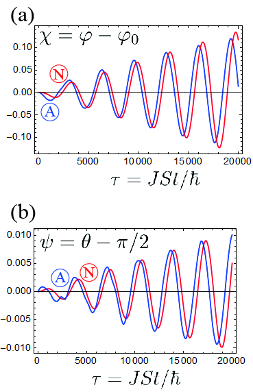
Figure 11: Time evolution of $\chi(L/2,\tau)$ and $\psi(L/2,\tau)$: numerical data (blue) and the analytical relation (49) and (48), respectively, (red) with $c_{\chi}=60$ and $c_{\psi}=-32$.

Finally, computation of $\tilde{\chi}$ and $\tilde{\psi}$ with the aid of the found solutions gives resonances of the Kittel ripples at $\Omega_{n}$. In Fig. 12, we summarize the results which are most essential results in this paper to make comparison between theoretical and experimental findings on the magnetic resonance in the case II.

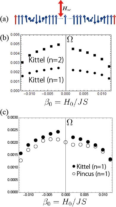
Figure 12: (a) Schematic view of the case II configuration. (b) Resonance frequencies for the Kittel ripples of the lowest orders $n=1$ and $n=2$ shown by $\CIRCLE$ and $\blacksquare$, respectively. (c) $H_{0}$-dependeces of the lowest antisymmetric ( $\Circle$ ) and the $n=1$ ripple ( $\CIRCLE$) modes.

In Fig. 12(c), it is seen that there appear double resonances. The lower branch originates from the Pincus mode and the upper branch originates from the Kittel ripple. Actually, the first and second resonance frequencies are reported as $\Omega_{1}\sim 17$GHz and $\Omega_{2}\sim 20$GHz with the bell-shaped field dependence, i.e., $(\Omega_{2}-\Omega_{1})/\Omega_{1}$ is the order of $0.1$. Based on this fact, we may conclude that the experimentally observed double resonances consistently correspond to the first Pincus mode and the first Kittel ripple mode, respectively. The difference in the resonance frequencies between the first and second Pincus modes [shown in Fig. 12(b)] is too large as compared with the experimental finding.

We also note that the intensities of the Pincus mode and Kittel ripples are almost similar, because they are both the fundamental modes. Based on these considerations, we may conclude that the resonance profile in the case II is attributed to the coexistence of the Pincus and Kittel excitations. In the final part ot Appendix C, we explained the reason why the resonance frequency for the Pincus mode is smaller than that of the Kittel ripple.

We also recognize an asymmetric profile of the distribution of the resonance frequencies with respect to the direction of the dc field ($\beta_{0}>0$ or $\beta_{0}<0$). This asymmetry is actually experimentally observed.Goncalves2017 The origin of this asymmetry is easily understood in terms of the uniform direction of the pinning field at both ends. Because the pinning fields $\boldsymbol{H}_{s}$ are uniform, the total field, $\boldsymbol{H}_{0}+\boldsymbol{H}_{s}$, exhibits an asymmetric profile depending on the orientation of $\boldsymbol{H}_{0}$, i.e., the $\boldsymbol{H}_{0}$ is either parallel to or antiparallel to the $\boldsymbol{H}_{s}$.

IV.2.2 SSW over the simple helix

As similar to the case I, the case of simple helix can be more easily analyzed than the case of the CSL. In the case II, the SSW is antisymmetric with respect to reflection across the center. This situation reminds us the standing waves in thin ferromagnetic films with the asymmetric surface pinning Puszkarski1973 . We accordingly modify the scheme given by Eqs. (27) and (28) in the form

$$\chi(z,\tau) =\frac{\sin(kz)}{\sin(kL/2)}\chi(L/2,\tau)+\varepsilon\tilde{\chi}(z,\tau),$$ (50)

$$\psi(z,\tau) =\frac{\sin(kz)}{\sin(kL/2)}\psi(L/2,\tau)+\varepsilon\tilde{\psi}(z,\tau).$$ (51)

Apparently, the boundary values become antisymmetric, $\chi(-L/2,\tau)=-\chi(L/2,\tau)$ and $\psi(-L/2,\tau)=-\psi(L/2,\tau)$, provided the short-range parts vanish at the ends.

We make use (50) and (51) for the system

$$\partial_{\tau}\psi =-\partial_{z}^{2}\chi+{\beta}_{x}(\tau)\sin(q_{s}z),$$ (52)

$$\partial_{\tau}\chi =\left[\partial_{z}^{2}-2({D}/{J})q_{s}+q_{s}^{2}\right]\psi,$$ (53)

and seek for the solution in the form of the Fourier series

$$\tilde{\psi}(z,\tau) =\sum_{n=1}^{\infty}\tilde{\psi}_{n}(\tau)\sin\left({2\pi nz}/{L}\right),$$ (54)

$$\tilde{\chi}(z,\tau) =\sum_{n=1}^{\infty}\tilde{\chi}_{n}(\tau)\sin\left({2\pi nz}/{L}\right).$$ (55)

Here,

$$\tilde{\chi}_{n}(\tau) =f_{n}\frac{\beta_{x0}}{\epsilon}\sqrt{\frac{q_{n}^{2}-q_{s}^{2}+2q_{s}(D/J)}{q_{n}^{2}}}$$

$$\times\frac{\left[\Omega_{n}\sin\left(\Omega\tau\right)-\Omega\sin\left(\Omega_{n}\tau\right)\right]}{\Omega^{2}-\Omega_{n}^{2}},$$ (56)

$$\tilde{\psi}_{n}(\tau)=f_{n}\frac{\beta_{x0}}{\epsilon}\Omega\,\frac{\left[\cos\left(\Omega_{n}\tau\right)-\cos\left(\Omega\tau\right)\right]}{\Omega^{2}-\Omega_{n}^{2}}$$ (57)

with the coefficients being given by

$$f_{n}=\frac{2}{L}\int_{-L/2}^{L/2}\sin\left(q_{s}z\right)\sin\left({2\pi nz}/{L}\right)dz.$$ (58)

The wavevectors are given by $q_{n}=2\pi n/L$ such that $\sin\left(q_{n}L/2\right)=0$. The resonance frequency for the Kittel ripple is then given by

$$\Omega_{n}^{2}=q_{n}^{2}\left[q_{n}^{2}-q_{s}^{2}+2q_{s}(D/J)\right].$$ (59)

On the other hand, the resonance frequency for the Pincus mode is obtained through

$$\left[k\cot(kL/2)\left(1-q_{s}D/J\right)+k^{2}/2+\beta_{s}\cos(kL/2)\right]$$

$$\times\left[k\cot(kL/2)+k^{2}/2-q_{s}^{2}/2\right.$$

$$\left.-(D/J)q_{s}+\beta_{s}\cos(kL/2)\right]$$

$$=k^{2}\left[k^{2}-q_{s}^{2}+2q_{s}(D/J)\right].$$ (60)

Numerical estimates with the same parameters as in the previous subsection give the value $k^{(2)}=0.0126038$. In Fig. 13, we show comparison between the numerical and analytical results.

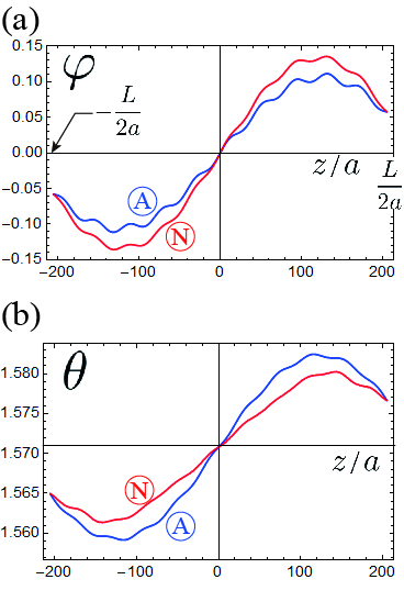
Figure 13: Comparison between numerical (red line) and analytical (blue line) results for the spatial profiles of (a) $\varphi$ and (b) $\theta$ associated with the second order standing waves over the helical structure under zero dc magnetic field ($\beta_{0}=0$). The parameters are taken as $\beta_{\text{s}}=0.02$ and $\beta_{x0}=0.0001$. Analytical result is obtained by Eqs. (50) and (51) with $\epsilon=-2/3$ at $\tau=9500$.

To specify boundary dynamics, we substitute

$$\chi(\bar{z},\tau)\sim c_{\chi}\frac{\sin(kz)}{\sin(kL/2)}\chi(L/2,\tau),$$ (61)

$$\psi(z,\tau)\sim c_{\psi}\frac{\sin(kz)}{\sin(kL/2)}\psi(L/2,\tau),$$ (62)

into Eqs. (9) and (10) that yields

$$\chi\left(z_{L/2},\tau\right) =\frac{\beta_{x0}}{c_{\chi}}\frac{B_{k}\sin\varphi_{0}(z_{L/2})}{\Omega_{0}\left(\Omega_{0}^{2}-\Omega^{2}\right)}\left[\Omega_{0}\sin\Omega\tau-\Omega\sin\Omega_{0}\tau\right],$$ (63)

$$\psi\left(z_{L/2},\tau\right) =\frac{\beta_{x0}}{c_{\psi}}\frac{\Omega\sin\varphi_{0}(z_{L/2})}{\left(\Omega^{2}-\Omega_{0}^{2}\right)}\left[\cos\Omega_{0}\tau-\cos\Omega\tau\right],$$ (64)

where

$$B_{k}=-k\cot(kL/2)-k^{2}/2+q_{s}^{2}/2+(D/J)q_{s}-\beta_{\text{s}}\cos(kL/2).$$ (65)

These results show that the end spins oscillate with the frequency of unperturbed standing wave

$$\Omega_{0}^{2}={k}^{2}\left[k^{2}-q_{s}^{2}+2q_{s}(D/J)\right],$$ (66)

where the numerical estimation gives $\Omega_{0}\approx 0.0020185$. For comparison, the lowest short-range ripple frequency is $\Omega_{1}=0.0024617$. Figs. 14(a), (b) illustrate comparison of (63) and (64) with numerical data.

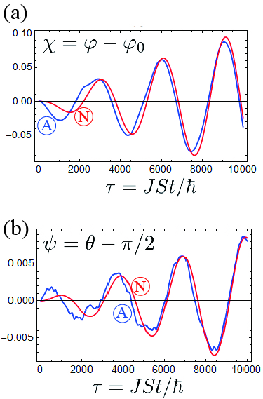
Figure 14: Time evolution of $\chi(L/2,\tau)$ and $\psi(L/2,\tau)$: numerical data (blue) compared to the analytical relations (49) and (48), respectively, (red) with $c_{\chi}=-12.5$ and $c_{\psi}=-19.0$.

V Discussions and conclusions

In this paper, motivated by experimental findings on the magnetic field-dependence of the resonance profile in CrNb₃S₆,Goncalves2017 we developed a theory of the SSW in a mono-axial chiral helimagnet. We assumed that micro-sized samples used in Ref.Goncalves2017 are described as thin films with both the surface end spins being softly pinned and constructed a theory along with the line of Kittel-Pincus theories of ferromagnetic resonance. From technical viewpoints, we presented a scheme of the Davis-Puszkarski equation generalized to the case of chiral helimagnetic structure under the static magnetic field applied perpendicular to the chiral axis.

Consequently, we found there are two classes of the SSW over the spatially modulated chiral spin soliton lattice state. One is the soft Pincus mode, while another is the hard Kittel ripple. The former is anologus to the SSW in a ferromagnetic thin film discussed by Pincus.Pincus1960 The latter appears only in the case of spatially modulated spin structure, because the spatially oscillating field acts on the interior spins and causes forced oscillation in space-domain. The Kittel ripples are excited only when the ac magnetic field is applied perpendicular to the chiral axis, because the perpendicular field couples with the spatially modulated component of the spins through the term $\beta_{x}(t)$cos$\varphi_{0}\left(z\right)$. The existence of two modes, Pincus modes and Kitttel ripples are consistent with the experimentally observed double resonance profile.

Standing spin waves in thin ferromagnetic films have been intensively studied from both theoretical and experimental standpoints. These excitations have already found a broad application in problems of spintronics. However, to best of our knowledge, problem on the SSW for noncolinear magnetic structure has not been addressed so far. The present paper may open a new direction in the field.

Finally, we make some general comments on the issues which have not been treated in this paper. Generally speaking, consideration on the chiral helimagnets requires careful treatment of dipole-exchange and magneto-static modes, which play an essential role in films of thickness typically in the range of micrometers.Damon1961 ; Hurben1995 ; Arias2016 Another important aspect involved in practical application of the standing spin waves pertains to accounting for damping effects not dealt with in this work. The theoretical studies for thin films of itinerant ferromagnet have shown that the Landau damping mechanism of the standing wave modes is sufficiently severe, since they have a finite and rather large vector normal to the film surfaces.Costa2004 An analysis of the perpendicular standing waves in sputtered permalloy films by means of a waveguide based FMR measurements identifies three contributions to their damping: the intrinsic damping, the eddy-current damping,Lock1966 and the radiative damping that stem from the inductive coupling between sample and the waveguide.Schoen2015 The radiative damping presents in all ferromagnets including insulators.

The eddy-current damping may be materialized for standing waves in CrNb₃S₆ films, since there are itinerant carriers from conducting NbS₂ layers. However, even studies in itinerant ferromagnets, quite thick permalloy films, demonstrate that the eddy-current damping may be neglected in higher order standing waves. In addition, in thin ferromagnetic films the eddy-current damping was found to be negligible in comparison with the wave-number-dependent damping mechanism due to intra-layer spin-current transport.Li2016 Further theoretical and experimental exploration toward this direction is of interest for future investigations.

Appendix A Lamé form of equations of motion

We here derive Eqs. (7) and (8). First, in Eqs. (3) and (4), we make linear expansion with respect to $\psi$ and $\chi$ to obtain

$$\sin\theta\partial_{z}^{2}\varphi \rightarrow\partial_{z}^{2}\varphi_{0}+\partial_{z}^{2}\chi,$$

$$\beta_{0}\sin\varphi \rightarrow\beta_{0}\sin\varphi_{0}+\left(\beta_{0}\cos\varphi_{0}\right)\chi,$$

$$\beta_{x}\sin\varphi \rightarrow\beta_{x}\sin\varphi_{0},$$

$$\sin\theta\cos\theta\left(\partial_{z}\varphi\right)^{2} \rightarrow-\psi\left(\partial_{z}\varphi_{0}\right)^{2},$$

$$\sin\theta\cos\theta\partial_{z}\varphi \rightarrow-\psi\partial_{z}\varphi_{0},$$

where we note $\varphi_{0}$ satisfies the sine-Gordon equation, $\partial_{z}^{2}\varphi_{0}=\beta_{0}\sin\varphi_{0}$. The higer order terms such as $\psi\partial_{z}\psi$, $\beta_{x}\chi$ and $\beta_{x}\psi$ are discarded ($\beta_{x}$ is treated as a small perturbation). Plugging them into Eqs. (3) and (4) and introducing dimensionless space and time variables, $\bar{z}=z\sqrt{\beta_{0}}/\kappa$ and $\tau=JSt/\hbar$, we have

$$\frac{\kappa^{2}}{\beta_{0}}\partial_{\tau}\psi =\left(-\frac{\partial^{2}}{\partial\bar{z}^{2}}+\kappa^{2}\cos\varphi_{0}\right)\chi+\frac{\kappa^{2}}{\beta_{0}}\beta_{x}(\tau)\sin\varphi_{0},$$ (67)

$$\frac{\kappa^{2}}{\beta_{0}}\partial_{\tau}\chi =-\left[-\frac{\partial^{2}}{\partial\bar{z}^{2}}+\kappa^{2}\cos\varphi_{0}-\left({\partial_{\bar{z}}\varphi}_{0}\right)^{2}\right.$$

$$\left.+2\frac{D}{J}\frac{\kappa}{\sqrt{\beta_{0}}}\left({\partial_{\bar{z}}}\varphi_{0}\right)\right]\psi-\frac{\kappa^{2}}{\beta_{0}}\beta_{z}(\tau).$$ (68)

Using Eq. (5), it may be shown

$$\cos\varphi_{0} =-1+2\text{sn}^{2}\bar{z},$$ (69)

$${\partial_{\bar{z}}}\varphi_{0} =2\text{dn}\bar{z}.$$ (70)

and Eq. (67) is reduced to Eq. (7). For small $\kappa$, we can approximate

$$\frac{\kappa}{\sqrt{\beta_{0}}} =\frac{4JE(\kappa)}{\pi D}\sim\frac{2J}{D}\left(1-\frac{\kappa^{2}}{4}\right),$$ (71)

$$\text{dn}\bar{z} =\sqrt{1-\kappa^{2}\text{sn}^{2}\bar{z}}\sim 1-\frac{\kappa^{2}}{2}\text{sn}^{2}\bar{z}.$$ (72)

Then, Eq. (68) is reduced to

$$\frac{\kappa^{2}}{\beta_{0}}\partial_{\tau}\chi =-\left(-\frac{\partial^{2}}{\partial\bar{z}^{2}}+2\kappa^{2}\text{sn}^{2}\bar{z}-3\kappa^{2}+4\right)\psi$$

$$-\frac{\kappa^{2}}{\beta_{0}}\beta_{z}(\tau),$$ (73)

which gives Eq. (8).

Appendix B Dynamics of the surface end spins

We examine in detail the motion of the end spins with the coordinates $\pm L/2$ in a line of $N$ spins along the $z$ axis. It is assumed that the end spins experience an effective ’surface’ anisotropy field $H_{\text{s}}$, the same on both ends, which is perpendicular to the line and to the static magnetic field $H_{0}$.

The boundary spins differ from interior ones in that they have only one nearest neighbour instead of the usual two, thereby giving the Hamiltonian for the right end spin

$$\mathcal{H}_{R} =-J\boldsymbol{S}_{L/2-1}\cdot\boldsymbol{S}_{L/2}-D\left[\boldsymbol{S}_{L/2-1}\times\boldsymbol{S}_{L/2}\right]_{z}$$

$$-\left(H_{0}+H_{\text{s}}\right)S_{L/2}^{x}.$$ (74)

The equations of motion are then shaped into

$$\partial_{\tau}\theta_{L/2} =\sin\theta_{L/2-1}\sin\left(\varphi_{L/2}-\varphi_{L/2-1}\right)$$

$$-\left(D/J\right)\sin\theta_{L/2-1}\cos\left(\varphi_{L/2}-\varphi_{L/2-1}\right)$$

$$+\left(\beta_{0}+\beta_{\text{s}}\right)\sin\varphi_{L/2},$$ (75)

$$\sin\theta_{L/2}\partial_{\tau}\varphi_{L/2}=\cos\theta_{L/2}\sin\theta_{L/2-1}\cos\left(\varphi_{L/2-1}-\varphi_{L/2}\right)$$

$$-\sin\theta_{L/2}\cos\theta_{L/2-1}$$

$$+\left(D/J\right)\cos\theta_{L/2}\sin\theta_{L/2-1}\sin\left(\varphi_{L/2}-\varphi_{L/2-1}\right)$$

$$+\left(\beta_{0}+\beta_{\text{s}}\right)\cos\theta_{L/2}\cos\varphi_{L/2}.$$ (76)

The system (9) and (10) originates from (75) and (76) in a continuum limit. Eq.(22) for the wave vector of the ground state is obtained if to take $\varphi_{i}=q_{s}z_{i}$ and $\theta_{i}=\pi/2$. A treatment for the left edge may be done in a similar way.

Appendix C General scheme of the Davis-Puszkarski equation for one-dimensional noncolinear magnetic structure

For convenience of applications to the standing spin wave problem in a non-colinear magnetic chain, we here give a concise summary of the Davis-Puszkarski equation in a self-contained manner. The notation in this appendix will be independent of that of the main body of the paper.

C.1 Equations of motion for the interior and the ends

We represent the arrangement of the spins on a chain with a linear length $L$ using the polar coordinates, $\boldsymbol{S}\left(z\right)=S\left(\sin\theta\cos\varphi,\sin\theta\sin\varphi,\cos\theta\right)$. The interior system is described by a Lagrangian in a general form,

$$L\left[\theta,\varphi\right]=\hbar S\int_{-\frac{L}{2}}^{\frac{L}{2}}\left(\cos\theta-1\right)\partial_{t}\varphi dz-\int_{-\frac{L}{2}}^{\frac{L}{2}}\mathcal{H}\left[\theta,\varphi\right]dz,$$ (77)

where the first term represents the kinetic Berry phase term. The effective Hamiltonian $\mathcal{H}\left[\theta,\varphi\right]$ describes a continuous model which contains spatial derivatives of $\theta$ and $\varphi$ fields coming from the exchange interactions and non-linear Zeeman terms such as $\sin\theta\cos\varphi$ or cos$\theta$. Then, the coupled Euler-Lagrangian equations of motion are written down to be

$$\hbar S\sin\theta\frac{\partial\theta}{\partial t} =\frac{\delta\mathcal{H}}{\delta\varphi},$$ (78)

$$\hbar S\sin\theta\frac{\partial\varphi}{\partial t} =-\frac{\delta\mathcal{H}}{\delta\theta}.$$ (79)

Next we assume that the ground state configuration $\theta_{0}\left(z\right)$ and $\varphi_{0}\left(z\right)$ are given through the stationarity condition $\delta\int\mathcal{H}\left[\theta,\varphi\right]dz=0$ and consider the small (Gaussian) fluctuations $\delta\theta\left(z,t\right)$ and $\delta\varphi\left(z,t\right)$,

$$\theta\left(z,t\right) =\theta_{0}\left(z\right)+\delta\theta\left(z,t\right),$$ (80)

$$\varphi\left(z,t\right) =\varphi_{0}\left(z\right)+\delta\varphi\left(z,t\right).$$ (81)

Expanding the EOMs (78) and (79), we may obtain the EOMs for the fluctuations in a general form,

$$\frac{\partial\delta\theta\left(z,t\right)}{\partial t} =\hat{\mathcal{L}}_{\varphi}\delta\varphi\left(z,t\right)+\epsilon f\left(z,t\right),$$ (82)

$$\frac{\partial\delta\varphi\left(z,t\right)}{\partial t} =-\hat{\mathcal{L}}_{\theta}\delta\theta\left(z,t\right),$$ (83)

where $\hat{\mathcal{L}}_{\varphi}$ and $\hat{\mathcal{L}}_{\theta}$ are linear differential operators. Without loss of generality, we introduce a small external force term $\epsilon f\left(z,t\right)$. From now on, we consider two cases: $\epsilon=0$ and finite $\epsilon\neq 0$.

Next we address to EOMs for the end spins. We start with the lattice Hamiltonian and write down the EOMs for the end spins, $\boldsymbol{S}_{1}$ and $\boldsymbol{S}_{N}$, which couple with the nearest neighbor interior spins $\boldsymbol{S}_{2}$ and $\boldsymbol{S}_{N-1}$, respectively. For example, the right-side end ($z=L/2$), the continuum limit is taken as

$$\varphi_{{}_{N-1}}\sim\varphi(L/2)-a\frac{\partial\varphi\left(z\right)}{\partial z}+\frac{a^{2}}{2}\frac{\partial^{2}\varphi\left(z\right)}{\partial z^{2}},$$ (84)

and then evaluating the derivative at $z=L/2$. Thus, we obtain the EOMs at the ends,

$$\frac{\partial\delta\theta_{\text{s}}\left(z,t\right)}{\partial t} =\hat{\mathcal{M}}_{\varphi}\delta\varphi_{\text{s}}\left(z,t\right)+\epsilon f\left(z,t\right),$$ (85)

$$\frac{\partial\delta\varphi_{\text{s}}\left(z,t\right)}{\partial t} =-\hat{\mathcal{M}}_{\theta}\delta\theta_{\text{s}}\left(z,t\right).$$ (86)

Here, $\hat{\mathcal{M}}_{\varphi}$ and $\hat{\mathcal{M}}_{\theta}$ are the linear operators including the effects of the surface pinning fields. After acting by these operators on $\delta\varphi_{\text{s}}\left(z,t\right)$ and $\delta\theta_{\text{s}}\left(z,t\right)$, respectively, we fix then $z=z_{\text{s}}=\pm L/2$, and, consequently, a dependence on the interior coordinate, $z$, disappears.

C.2 The case of $\epsilon=0$

In the case of $\epsilon=0$, Eqs. (82) and (83) are solved using separation of variables,

$$\delta\theta\left(z,t\right) =\mu\left(z\right)M\left(t\right),$$ (87)

$$\delta\varphi\left(z,t\right) =\nu\left(z\right)N\left(t\right).$$ (88)

Inserting these forms to Eqs. (82) and (83), we obtain

$$\frac{1}{N\left(t\right)}\frac{\partial M\left(t\right)}{\partial t} =\frac{1}{\mu\left(z\right)}\hat{\mathcal{L}}_{\varphi}\nu\left(z\right)=C_{1},$$ (89)

$$\frac{1}{M\left(t\right)}\frac{\partial N\left(t\right)}{\partial t} =-\frac{1}{\nu\left(z\right)}\hat{\mathcal{L}}_{\theta}\mu\left(z\right)=-C_{2},$$ (90)

with $C_{1}$ and $C_{2}$ being constants. Then the temporal constituents immediately gives the eigenfrequency for the interior system,

$$\Omega_{\text{interior}}=\sqrt{C_{1}C_{2}}.$$ (91)

Next let us consider the spatial parts,

$$\hat{\mathcal{L}}_{\varphi}\nu\left(z\right) =C_{1}\mu\left(z\right),$$ (92)

$$\hat{\mathcal{L}}_{\theta}\mu\left(z\right) =C_{2}\nu\left(z\right).$$ (93)

Here we assume that the differential operators $\hat{\mathcal{L}}_{\theta}$ and $\hat{\mathcal{L}}_{\varphi}$ have simultaneous eigenfunctions, $\Psi_{q}\left(z\right)$, labeled by an index $q$. That is to say,

$$\hat{\mathcal{L}}_{\theta}\Psi_{q}\left(z\right) =\lambda_{\theta}\left(q\right)\Psi_{q}\left(z\right),$$ (94)

$$\hat{\mathcal{L}}_{\varphi}\Psi_{q}\left(z\right) =\lambda_{\varphi}\left(q\right)\Psi_{q}\left(z\right)..$$ (95)

Expanding $\mu\left(z\right)$ and $\nu\left(z\right)\$in terms of $\Psi_{q}\left(z\right)$ as the orthogonal basis,

$$\mu\left(z\right) ={\textstyle\sum_{q}}\mu_{q}\Psi_{q}\left(z\right),$$ (96)

$$\nu\left(z\right) ={\textstyle\sum_{q}}\nu_{q}\Psi_{q}\left(z\right),$$ (97)

we have

$${\textstyle\sum_{q}}\left[\nu_{q}\lambda_{\varphi}\left(q\right)-C_{1}\mu_{q}\right]\Psi_{q}\left(z\right) =0,$$ (98)

$${\textstyle\sum_{q}}\left[\mu_{q}\lambda_{\theta}\left(q\right)-C_{2}\nu_{q}\right]\Psi_{q}\left(z\right) =0,$$ (99)

which lead to

$$C_{1}=\frac{\nu_{q}}{\mu_{q}}\lambda_{\varphi}\left(q\right)\text{, }C_{2}=\frac{\mu_{q}}{\nu_{q}}\lambda_{\theta}\left(q\right)\text{.}$$ (100)

Therefore, we can replace Eq. (91) with

$$\Omega_{\text{interior}}\left(q\right)=\sqrt{\lambda_{\theta}\left(q\right)\lambda_{\varphi}\left(q\right)}.$$ (101)

Now, let us turn attention to the fluctuations at the ends, described in a form

$$\delta\theta_{\text{s}}\left(t\right) =\delta\theta\left(z_{\text{s}},t\right)=c_{1}\Psi_{q}\left(z_{\text{s}}\right)M_{\text{s}}\left(t\right),$$ (102)

$$\delta\varphi_{\text{s}}\left(t\right) =\delta\varphi\left(z_{\text{s}},t\right)=c_{2}\Psi_{q}\left(z_{\text{s}}\right)N_{\text{s}}\left(t\right),$$ (103)

with $c_{1}$ and $c_{2}$ being constants, and $z_{\text{s}}=\pm L/2$. Note that the surface states ‘participate in’ or ‘swallowed up by’ the interior mode specified by $q$. Inserting them into Eqs. (85) and (86), we may have

$$\frac{\partial M_{\text{s}}\left(t\right)}{\partial t} =A_{q}N_{\text{s}}\left(t\right),$$ (104)

$$\frac{\partial N_{\text{s}}\left(t\right)}{\partial t} =-B_{q}M_{\text{s}}\left(t\right),$$ (105)

where  $A_{q}$ and $B_{q}$ contain spatial derivatives of $\Psi_{q}\left(z\right)$ at $z=z_{\text{s}}$, i.e., no liner differential operator appears. We dropped an external force term, since information on $A_{q}$ and $B_{q}$ is enough to obtain the Larmor frequency of the surface end spins,,

$$\Omega_{\text{surface}}(q)=\sqrt{A_{q}B_{q}}.$$ (106)

Now, the matching condition

$$\Omega_{n}\equiv\Omega_{\text{surface}}(q_{n})=\Omega_{\text{interior}}(q_{n})$$ (107)

gives the Davis-Puszkarski equation which determines a series of allowed values of $q_{n}$, ($n=1,2,\cdots$) corresponding to the SSW modes. In the context of this paper, this corresponds to the Pincus mode.

C.3 The case of $\epsilon\neq 0$

The existence of space-time dependent term $\epsilon f\left(z,t\right)$ prevents us from using separation of variables. We then seek for the interior solution in a perturbative manner based on an ansatz,

$$\delta\theta\left(z,t\right) =\frac{\mu\left(z\right)}{\mu_{\text{s}}}\delta\theta_{\text{s}}\left(t\right)+\epsilon\tilde{\psi}\left(z,t\right),$$ (108)

$$\delta\varphi\left(z,t\right) =\frac{\nu\left(z\right)}{\nu_{\text{s}}}\delta\varphi_{\text{s}}\left(t\right)+\epsilon\tilde{\chi}\left(z,t\right),$$ (109)

where $\mu_{\text{s}}$ and $\nu_{\text{s}}$ are respectively the values of $\mu\left(z\right)$ and $\nu\left(z\right)$ at the surface ends. In this ansatz, we implicitly assume that the time-dependence at the surface, $\delta\theta_{\text{s}}\left(t\right)$ and $\delta\varphi_{\text{s}}\left(t\right)$, are known. We here impose the boundary condition,

$$\tilde{\psi}\left(z_{\text{s}},t\right)=\tilde{\chi}\left(z_{\text{s}},t\right)=0,$$ (110)

which means the perfect pinning of the $\tilde{\chi}$ and $\tilde{\psi}$ fields at the ends. Due to these conditions, we consistently reproduce

$$\delta\theta\left(z_{\text{s}},t\right) =\delta\theta_{\text{s}}\left(t\right),$$ (111)

$$\delta\varphi\left(z_{\text{s}},t\right) =\delta\varphi_{\text{s}}\left(t\right),$$ (112)

at the surfaces.

C.3.1 Pincus mode

Now, we proceed with analysis in a perturbative manner. Collecting the zeroth order terms with respect to $\epsilon$, we have

$$\frac{1}{\delta\varphi_{\text{s}}\left(t\right)}\frac{\partial\delta\theta_{\text{s}}\left(t\right)}{\partial t} =\frac{\mu_{\text{s}}}{\nu_{\text{s}}}\frac{1}{\mu\left(z\right)}\hat{\mathcal{L}}_{\varphi}\nu\left(z\right)=D_{1},$$ (113)

$$\frac{1}{\delta\theta_{\text{s}}\left(t\right)}\frac{\partial\delta\varphi_{\text{s}}\left(t\right)}{\partial t} =-\frac{\nu_{\text{s}}}{\mu_{\text{s}}}\frac{1}{\nu\left(z\right)}\hat{\mathcal{L}}_{\theta}\mu\left(z\right)=-D_{2},$$ (114)

with $D_{1}$ and $D_{2}$ being constants. Then, as in the case of $\epsilon=0$, the eigenfrequency for the interior system is given by

$$\Omega_{\text{interior}}\left(q\right)=\sqrt{D_{1}D_{2}}=\sqrt{\lambda_{\varphi}\left(q\right)\lambda_{\theta}\left(q\right)}.$$ (115)

Let us then turn attention to the surface spins. In the vicinity of the ends, $\tilde{\psi}\left(z,t\right)$ and $\tilde{\chi}\left(z,t\right)$ can be dropped and we have

$$\delta\theta\left(z,t\right) =c_{1}\Psi_{q}\left(z\right)\delta\theta_{\text{s}}\left(t\right).$$ (116)

$$\delta\varphi\left(z,t\right) =c_{2}\Psi_{q}\left(z\right)\delta\varphi_{\text{s}}\left(t\right),$$ (117)

with $c_{1}$ and $c_{2}$ being constants. It is to be noted that the basis function $\Psi_{q}\left(z\right)$ is now specified just as in the case of (102) and (103). Inserting them into Eqs. (85) and (86), we obtain the zeroth order equations,

$$\frac{\partial\delta\theta_{\text{s}}\left(t\right)}{\partial t} =\frac{c_{2}}{c_{1}}F_{q}\delta\varphi_{\text{s}}\left(t\right),$$ (118)

$$\frac{\partial\delta\varphi_{\text{s}}\left(t\right)}{\partial t} =-\frac{c_{1}}{c_{2}}G_{q}\delta\theta_{\text{s}}\left(t\right),$$ (119)

where $F_{q}$ and $G_{q}$ contain spatial derivatives of $\Psi_{q}\left(z\right)$ at $z=z_{\text{s}}$. We thus obtain the Larmor frequency of the surface end spins,

$$\Omega_{\text{surface}}\left(q\right)=\sqrt{F_{q}G_{q}}.$$ (120)

Now, again the matching condition

$$\Omega_{n}\equiv\Omega_{\text{surface}}\left(q_{n}\right)=\Omega_{\text{interior}}\left(q_{n}\right)$$ (121)

again gives the Davis-Puszkarski equation. In the context of this paper, this corresponds to the Pincus mode.

C.3.2 Kittel ripple

Next, we consider the first order terms to obtain

$$\frac{\partial\tilde{\psi}\left(z,t\right)}{\partial t} =\hat{\mathcal{L}}_{\varphi}\tilde{\chi}\left(z,t\right)+f\left(z,t\right),$$ (122)

$$\frac{\partial\tilde{\chi}\left(z,t\right)}{\partial t} =-\hat{\mathcal{L}}_{\theta}\tilde{\psi}\left(z,t\right),$$ (123)

where the linear operators, $\hat{\mathcal{L}}_{\varphi}$ and $\hat{\mathcal{L}}_{\theta}$, for the interior system appear. Again, we expand $\tilde{\psi}\left(z,t\right)$ and $\tilde{\chi}\left(z,t\right)\$in terms of $\Psi_{Q}\left(z\right)$,

$$\tilde{\psi}\left(z,t\right) ={\textstyle\sum_{Q}}\tilde{\psi}_{Q}\left(t\right)\Psi_{Q}\left(z\right),$$ (124)

$$\tilde{\chi}\left(z,t\right) ={\textstyle\sum_{Q}}\tilde{\chi}_{Q}\left(t\right)\Psi_{Q}\left(z\right).$$ (125)

In this case, the allowed $Q$ is determined solely by the perfect pinning condition

$$\Psi_{Q_{n}}\left(z_{\text{s}}\right)=0.$$ (126)

We should note the essential difference between the conditions (121) and (126).

We insert Eqs. (124) and (125) into Eqs. (122) and (123), take one more time derivative, multiply the both sides by $\Psi_{Q}\left(z\right)$, and integrate over $z$ to obtain

$$\frac{d^{2}\tilde{\psi}_{Q}\left(t\right)}{dt^{2}} =-\lambda_{\theta}\left(Q\right)\lambda_{\varphi}\left(Q\right)\tilde{\psi}_{Q}\left(t\right)+\frac{df_{Q}\left(t\right)}{dt},$$ (127)

$$\frac{d^{2}\tilde{\chi}_{Q}\left(t\right)}{dt^{2}} =-\lambda_{\varphi}\left(Q\right)\lambda_{\theta}\left(Q\right)\tilde{\chi}_{Q}\left(t\right)-\lambda_{\theta}\left(Q\right)f_{Q}\left(t\right),$$ (128)

where

$$f_{Q}\left(t\right)=\frac{\int_{-L/2}^{L/2}\Psi_{Q}\left(z\right)f\left(z,t\right)dz}{\int_{-L/2}^{L/2}\Psi_{Q}^{2}\left(z\right)dz}.$$ (129)

Now the the eigenfrequency,

$$\tilde{\Omega}_{n}=\sqrt{\lambda_{\theta}\left(Q_{n}\right)\lambda_{\varphi}\left(Q_{n}\right)},$$ (130)

specifies the modes associates with $\tilde{\psi}\left(z,t\right)$ and $\tilde{\chi}\left(z,t\right),$ i.e., the Kittel ripple in the present context. Eqs. (127) and (128) are readily solved to give

$$\tilde{\psi}_{Q_{n}}\left(t\right) =\frac{1}{\tilde{\Omega}_{n}}\int_{0}^{t}\frac{df_{Q}\left(t^{\prime}\right)}{dt^{\prime}}\sin[\tilde{\Omega}_{n}(t-t^{\prime})]dt^{\prime},$$ (131)

$$\tilde{\chi}_{Q_{n}}\left(t\right) =-\frac{\tilde{\lambda}_{\theta}\left(Q\right)}{\tilde{\Omega}_{n}}\int_{0}^{t}f_{Q}\left(t^{\prime}\right)\sin[\tilde{\Omega}_{n}(t-t^{\prime})]dt^{\prime},$$ (132)

provided $f_{Q}(0)=0$. Finally, we note

$$\Omega_{n}<\tilde{\Omega}_{n},$$ (133)

because the Kittel modes, $\tilde{\psi}\left(z,t\right)$ and $\tilde{\chi}\left(z,t\right)$, are strictly confined into the system over the region $-L/2\leq z\leq L/2$. On the other hand, the Pincus mode can be extended beyond this region. This makes $\Omega_{n}$ smaller than $\tilde{\Omega}_{n}$ for a common $n$.

References

- (1) A. Barman and J. Sinha, Spin Dynamics and Damping in Ferromagnetic Thin Films and Nanostructures (Springer, Cham, Switzerland, 2018).
- (2) Y. Togawa, T. Koyama, K. Takayanagi, S. Mori, Y. Kousaka, J. Akimitsu, S. Nishihara, K. Inoue, A. S. Ovchinnikov, and J. Kishine, Phys. Rev. Lett. 108, 107202 (2012).
- (3) Y. Togawa, Y. Kousaka, S. Nishihara, K. Inoue, J. Akimitsu, A.S. Ovchinnikov, and J. Kishine, Phys. Rev. Lett. 111, 197204 (2013).
- (4) L. Wang, N. Chepiga, D.- K. Ki, L. Li, F. Li, W. Zhu, Y. Kato, O.S. Ovchinnikova, F. Mila, I. Martin, D. Mandrus, and A.F. Morpurgo, Phys. Rev. Lett. 118, 257203 (2017).
- (5) Y. Togawa, T. Koyama, Y. Nishimori, Y. Matsumoto, S. McVitie, D. McGrouther, R.L. Stamps, Y. Kousaka, J. Akimitsu, S. Nishihara, K. Inoue, I.G. Bostrem, V.E. Sinitsyn, A.S. Ovchinnikov, and J. Kishine, Phys. Rev. B 92, 220412 (2015).
- (6) J. Kishine and A. S. Ovchinnikov, Solid State Phys. 66, 1 (2015).
- (7) J. Kishine, I. Proskurin, I. G. Bostrem, A. S. Ovchinnikov, and Vl. E. Sinitsyn, Phys. Rev. B 93, 054403 (2016).
- (8) F. J. T. Goncalves, T. Sogo, Y. Shimamoto, Y. Kousaka, J. Akimitsu, S. Nishihara, K. Inoue, D. Yoshizawa, M. Hagiwara, M. Mito, R. L. Stamps, I. G. Bostrem, V. E. Sinitsyn, A. S. Ovchinnikov, J. Kishine, and Y. Togawa, Phys. Rev. B 95, 104415 (2017).
- (9) F. J. T. Goncalves, T. Sogo, Y. Shimamoto, I. Proskurin, Vl. E. Sinitsyn, Y. Kousaka, I. G. Bostrem, J. Kishine, A. S. Ovchinnikov, and Y. Togawa, Phys. Rev. B 98, 144407 (2018).
- (10) C. Kittel, Phys. Rev. 110, 1295 (1958).
- (11) P. Pincus, Phys. Rev. 118, 658 (1960).
- (12) J.R. Davis, and F. Keffer, J. Appl. Phys. 34, 1135 (1963).
- (13) H. Puszkarski, IEEE Trans. Magn. 9, 22 (1973).
- (14) J.R. Banavar, and F. Keffer, Phys. Rev. B 17, 2974 (1978).
- (15) M.H. Seavey, Jr. and P.E. Tannenwald, Phys. Rev. Lett. 1, 168 (1958).
- (16) S. E. Lofland, S. M. Bhagat, C. Kwon, M. C. Robson, R. P. Sharma, R. Ramesh, and T. Venkatesan, Physics Letters A 209, 246 (1995).
- (17) M. Mruczkiewicz, M. Krawczyk, V. K. Sakharov, Yu. V. Khivintsev, Yu. A. Filimonov, and S. A. Nikitov, J. Appl. Phys. 113, 093908 (2013).
- (18) M. P. Wismayer, B.W. Southern, X. L. Fan, Y. S. Gui, C.-M. Hu, and R. E. Camley, Phys. Rev. B 85, 064411 (2012).
- (19) P. Buczek, A. Ernst, and L. M. Sandratskii, Phys. Rev. Lett. 105, 097205 (2010).
- (20) A.A. Serga, A.V. Chumak, A. Andre, G.A. Melkov, A.N. Slavin, S.O. Demokritov, and B. Hillebrands, Phys. Rev. Lett. 99, 227202 (2007).
- (21) A. V. Chumak, A. A. Serga, B. Hillebrands, G. A. Melkov, V. Tiberkevich, and A. N. Slavin, Phys. Rev. B 79, 014405 (2009).
- (22) S. Klingler, V. Amin, S. Geprägs, K. Ganzhorn, H. Maier-Flaig, M. Althammer, H. Huebl, R. Gross, R. D. McMichael, M. D. Stiles, S. T.B. Goennenwein, and M. Weiler, Phys. Rev. Lett. 120, 127201 (2018).
- (23) R. Magaraggia, K. Kennewell, M. Kostylev, R. L. Stamps, M. Ali, D. Greig, B. J. Hickey, and C. H. Marrows, Phys. Rev. Lett. 83, 054405 (2011).
- (24) J. Kishine, I. G. Bostrem, A. S. Ovchinnikov, and Vl. E. Sinitsyn, Phys. Rev. B 89, 014419 (2014).
- (25) M. N. Wilson, E. A. Karhu, D. P. Lake, A. S. Quigley, S. Meynell, A. N. Bogdanov, H. Fritzsche, U. K. Rößler, and T. L. Monchesky, Phys. Rev. B 88, 214420 (2013).
- (26) R. F. Soohoo, Phys. Rev. 131, 594 (1963).
- (27) G. Rado and J. Weertman, J. Phys. Chem. Solids 11, 315 (1959).
- (28) M. Sparks, Phys. Rev. B 1, 3831 (1970).
- (29) M. Shinozaki1, S. Hoshino, Y. Masaki, J. Kishine, and Y. Kato, J. Phys. Soc. Jpn. 85, 074710 (2016).
- (30) I. E. Dzyaloshinskii, Zh. Eksp. Teor. Fiz. 46, 1420 (1964) [Sov. Phys. JETP 19, 960 (1964)]; Zh. Eksp. Teor. Fiz. 47, 992 (1964) [Sov. Phys. JETP 20, 665 (1965)].
- (31) J. Kishine and A. S. Ovchinnikov, Phys. Rev. B 79, 220405(R) (2009).
- (32) J. Kishine, I. G. Bostrem, A. S. Ovchinnikov, and Vl. E. Sinitsyn, Phys. Rev. B 86, 214426 (2012).
- (33) We use Kittel’s terminology here, where the SSW order corresponds to a number of half-wavelengths on a line.
- (34) A. Polyanin, Handbook of Linear Partial Differential Equations for Engineers and Scientists (Chapman Hall/CRC, Boca Raton, FL, 2002). Section 0.11.1 therein.
- (35) R. W. Damon and J. R. Eshbach, J. Phys. Chem. Solids 19, 308 (1961).
- (36) M. J. Hurben and C. E. Patton, J. Magn. Magn. Mater. 139, 263 (1995).
- (37) R. E. Arias , Phys. Rev. B 94, 134408 (2016).
- (38) A. T. Costa, R. B. Muniz, and D. L. Mills, Phys. Rev. B 69, 064413 (2004).
- (39) J.M. Lock, Br. J. Appl. Phys. 17, 1645 (1966).
- (40) M. A. W. Schoen, J. M. Shaw, H. T. Nembach, M. Weiler, and T. J. Silva, Phys. Rev. B 92, 184417 (2015).
- (41) Y. Li and W.E. Bailey, Phys. Rev. Lett. 116, 117602 (2016).