Bayesian Heatmaps: Probabilistic Classification with Multiple Unreliable Information Sources

Abstract

Unstructured data from diverse sources, such as social media and aerial imagery, can provide valuable up-to-date information for intelligent situation assessment. Mining these different information sources could bring major benefits to applications such as situation awareness in disaster zones and mapping the spread of diseases. Such applications depend on classifying the situation across a region of interest, which can be depicted as a spatial “heatmap". Annotating unstructured data using crowdsourcing or automated classifiers produces individual classifications at sparse locations that typically contain many errors. We propose a novel Bayesian approach that models the relevance, error rates and bias of each information source, enabling us to learn a spatial Gaussian Process classifier by aggregating data from multiple sources with varying reliability and relevance. Our method does not require gold-labelled data and can make predictions at any location in an area of interest given only sparse observations. We show empirically that our approach can handle noisy and biased data sources, and that simultaneously inferring reliability and transferring information between neighbouring reports leads to more accurate predictions. We demonstrate our method on two real-world problems from disaster response, showing how our approach reduces the amount of crowdsourced data required and can be used to generate valuable heatmap visualisations from SMS messages and satellite images.

1 Introduction

Social media enables members of the public to post real-time text messages, videos and photographs describing events taking place close to them. While many posts may be extraneous or misleading, social media nonetheless provides streams of up-to-date information across a wide area. For example, after the Haiti 2010 earthquake, Ushahidi gathered thousands of text messages that provided valuable first-hand information about the disaster situation [14]. An effective way to extract information from large unstructured datasets such as these is to employ crowds of non-expert annotators, as demonstrated by Galaxy Zoo[10]. Besides social media, crowdsourcing provides a means to obtain geo-tagged annotations from other unstructured data sources such as imagery from satellites or unmanned aerial vehicles (UAV).

In scenarios such as disaster response, we wish to infer the situation across a region of interest by combining annotations from multiple information sources. For example, we may wish to determine which areas are currently flooded, the level of damage to buildings in an earthquake zone, or the type of terrain in a specific area from a combination of SMS reports and satellite imagery. The situation across an area of interest can be visualised using a heatmap (e.g. Google Maps heatmap layer), which overlays colours onto a map to indicate the intensity or probability of phenomena of interest. Probabilistic methods have been used to generate heatmaps from observations at sparse, point locations[9, 1, 8], using a Bayesian treatment of Poisson process models. However, these approaches model the rate of occurrence of events, so are not suitable for classification problems. Instead, a Gaussian process (GP) classifier can be used to model a class label that varies smoothly over space or time. This uses a latent function over input coordinates, which is mapped through a sigmoid function to obtain probabilities[16]. However, standard GP classifiers are unsuitable for heterogeneous, crowdsourced data since they do not account for the differing relevance, error rates and bias of individual information sources and annotators.

A key challenge in exploiting crowdsourced information is to account for its unreliability and combine it with trusted data as it becomes available, such as reports from experienced first responders in a disaster zone. For regression problems, differing levels of accuracy can be handled using sensor fusion approaches such as [12, 25]. The approach of [25] uses heteroskedastic GPs to produce heatmaps that account for sensor accuracy through variance scaling. This method could be applied to spatial classification by mapping GPs through a softmax function. However, such an approach cannot handle label bias or accuracy that depends on the true class. Recently, [11], proposed learning a GP classifier from crowdsourced annotations, but their method uses a coin-flipping noise model that would suffer from the same drawbacks as adapting [25]. Furthermore they train the model using a maximum likelihood (ML) approach, which may incorrectly estimate reliability when data for some workers is insufficient[20, 17, 7].

For classification problems, each information source can be modelled by a confusion matrix [3], which quantifies the likelihood of observing a particular annotation from an information source given the true class label. This approach naturally accounts for bias toward a particular answer and varying accuracy depending on the true class, and has been shown to outperform techniques such as majority voting and weighted sums[20, 17, 7]. Recent extensions following the Bayesian treatment of [7] can further improve results: by identifying clusters of crowd workers with shared confusion matrices [13, 23]; accounting for the time each worker takes to complete a task[24]; additionally modelling language features in text classification tasks[4, 21]. However, these methods depend on receiving multiple labels from different workers for the same data points, or, in the case of [4, 21], on correlations between text features and target classes. None of the existing confusion matrix-based approaches can model the spatial distribution of each class, and therefore, when reports are sparsely distributed over an area of interest, they cannot compensate for the lack of data at each location.

In this paper, we propose a novel Bayesian approach to aggregating sparse, geo-tagged reports from sources of varying reliability, which combines independent Bayesian classifier combination (IBCC) [7] with a GP classifier to infer discrete state values across an area of interest. Our model, HeatmapBCC, assumes that states at neighbouring locations are correlated, allowing us to fuse neighbouring reports and interpolate between them to predict the state at locations with no reports. HeatmapBCC uses confusion matrices to model the error rates, relevance and bias of each information source, permitting the use of non-expert crowds providing heterogeneous annotations. The GP handles the uncertainty that arises from sparse spatial data in a principled Bayesian manner, allowing us to incorporate prior information, such as physical models of disaster events such as earthquakes, and visualise the resulting posterior distribution as a spatial heatmap. We derive a variational inference method that is able to learn the reliability model for each information source without the need for ground truth training data. This method learns full distributions over latent variables that can be used to prioritise locations for further data gathering using an active learning approach. The next section presents in detail the HeatmapBCC model, and provides details of our efficient approximate inference algorithm. The following section then provides an empirical evaluation of our method on both synthetic and real-world problems, showing that HeatmapBCC can outperform rival methods. We make our code publicly available at https://github.com/OxfordML/heatmap_expts.

2 The HeatmapBCC Model

Our goal is to classify locations of interest, e.g. to identify them as “flooded” or “not flooded”. We can then choose locations in a grid over an area of interest and plot the classifications on a map as a spatial heatmap. The task is to infer a vector $\boldsymbol{t}^{*}\in\{1,..,J\}^{N^{*}}$ of target state values at $N^{*}$ locations $\boldsymbol{X}^{*}$, where $J$ is the number of state values or classes. Each row $\boldsymbol{x}_{i}$ of matrix $\boldsymbol{X}^{*}$ is a coordinate vector that specifies a point on the map. We observe a matrix of potentially unreliable geo-tagged reports, $\boldsymbol{c}\in\{1,..,L\}^{N\times S}$, with $L$ possible discrete values, from $S$ different information sources at $N$ training locations $\boldsymbol{X}$.

HeatmapBCC assumes that each report label $c_{i}^{(s)}$, from information source $s$, at location $\boldsymbol{x}_{i}$, is drawn from $c_{i}^{(s)}|t_{i},\boldsymbol{\pi}^{(s)}\sim\mathrm{Categorical}(\boldsymbol{\pi}_{t_{i}}^{(s)})$. The target state, $t_{i}$, selects the row, $\boldsymbol{\pi}_{t_{i}}^{(s)}$, of a confusion matrix[3, 20], $\boldsymbol{\pi}^{(s)}$, which describes the errors and biases of $s$ as a dependency between the report labels and the ground truth state, $t_{i}$. As per standard IBCC [7], the reports from each information source are conditionally independent of one another given target $t_{i}$, and each row of the confusion matrix is drawn from $\boldsymbol{\pi}_{j}^{(s)}|\boldsymbol{\alpha}_{0,j}^{(s)}\sim\mathrm{Dirichlet}(\boldsymbol{\alpha}_{0,j}^{(s)})$. The hyperparameters $\boldsymbol{\alpha}_{0,j}^{(s)}$ encode the prior trust in $s$.

We assume that state $t_{i}$ at location $\boldsymbol{x}_{i}$ is drawn from a categorical distribution, $t_{i}|\boldsymbol{\rho}_{i}\sim\mathrm{Categorical}(\boldsymbol{\rho}_{i})$, where $\rho_{i,j}=p(t_{i}=j|\boldsymbol{\rho}_{i})\in[0,1]$ is the probability of state $j$ at location $\boldsymbol{x}_{i}$. The generative process for state probabilities, $\boldsymbol{\rho}$, is as follows. First, draw latent functions for classes $j\in\{1,..,J\}$ from a Gaussian process prior: $f_{j}\sim\mathcal{GP}(m_{j},k_{j,\boldsymbol{\theta}}/\varsigma_{j})$, where $m_{j}$ is the prior mean function, $k_{j}$ is the prior covariance function, $\boldsymbol{\theta}$ are hyperparameters of the covariance function, and $\varsigma_{j}$ is the inverse scale. Map latent function values $f_{j}(\boldsymbol{x}_{i})\in\mathcal{R}$ to state probabilities: $\boldsymbol{\rho}_{i}=\sigma(f_{1}(\boldsymbol{x}_{i}),..,f_{J}(\boldsymbol{x}_{i}))\in[0,1]^{J}$. Appropriate functions for $\sigma$ include the logistic sigmoid and probit functions for binary classification, and softmax and multinomial probit for multi-class classification. We assume that $\varsigma_{j}$ is drawn from a conjugate gamma hyperprior, $\varsigma_{j}\sim\mathcal{G}\left(a_{0},b_{0}\right)$, where $a_{0}$ is a shape parameter and $b_{0}$ is the inverse scale.

While the reports, $c_{i}^{(s)}$, are modelled in the same way as standard IBCC [7], HeatmapBCC introduces a location-specific state probability, $\boldsymbol{\rho}_{i}$, to replace the global class proportions, $\boldsymbol{\kappa}$, which IBCC [20] assumes are constant for all locations. Using a Gaussian process prior means the state probability varies reasonably smoothly between locations, thereby encoding correlations in the distribution over states at neighbouring locations. The covariance function is chosen to suit the scenario we wish to model and may be tailored to specific spatial phenomena (the geo-spatial impact of an earthquake, for example). The hyperparameters, $\boldsymbol{\theta}$, typically include a length-scale, $l$, which controls the smoothness of the function. Here, we assume a stationary covariance function of the form $k_{j,\boldsymbol{\theta}}\left(\boldsymbol{x},\boldsymbol{x}^{\prime}\right)=k_{j}\left(|\boldsymbol{x}-\boldsymbol{x}^{\prime}|,l\right)$, where $k$ is a function of the distance between two points and the length-scale, $l$. The joint distribution for the complete model is:

$$p\left(\boldsymbol{c},\boldsymbol{t},\boldsymbol{f}_{1},..,\boldsymbol{f}_{J},\boldsymbol{\varsigma}_{1},..,\boldsymbol{\varsigma}_{J},\boldsymbol{\pi}^{(1)}\!,...,\boldsymbol{\pi}^{(S)}|\boldsymbol{\mu}_{1},..,\boldsymbol{\mu}_{J},\boldsymbol{K}_{1},..,\boldsymbol{K}_{J},\boldsymbol{\alpha}_{0}^{(1)}\!,..,\boldsymbol{\alpha}_{0}^{(S)}\right)=$$

$$\prod_{i=1}^{N}\!\left\{\rho_{i,t_{i}}\!\prod_{s=1}^{S}\pi^{(s)}_{t_{i},c_{i}^{(s)}}\!\right\}\prod_{j=1}^{J}\left\{p\left(\boldsymbol{f}_{j}|\boldsymbol{\mu}_{j},\boldsymbol{K}_{j}/\varsigma_{j}\right)p\left(\varsigma_{j}|a_{0},b_{0}\right)\prod_{s=1}^{S}p\left(\boldsymbol{\pi}^{(s)}_{j}|\boldsymbol{\alpha}^{(s)}_{0,j}\right)\right\},$$

where $\boldsymbol{f}_{j}=\left[f_{j}(\boldsymbol{x}_{1}),..,f_{j}(\boldsymbol{x}_{N})\right]$, $\boldsymbol{\mu}_{j}=\left[m_{j}(\boldsymbol{x}_{1}),..,m_{j}(\boldsymbol{x}_{N})\right]$, and $\boldsymbol{K}_{j}\in\mathbb{R}^{N\times N}$ with elements $K_{j,n,{n^{\prime}}}=k_{j,\boldsymbol{\theta}}(\boldsymbol{x}_{n},\boldsymbol{x}_{n^{\prime}})$.

3 Variational Inference for HeatmapBCC

We use variational Bayes (VB) to efficiently approximate the posterior distribution over all latent variables, allowing us to handle streaming data reports online by restarting the VB algorithm from the previous estimate as new reports are received. To apply variational inference, we replace the exact posterior distribution with a variational approximation that factorises into separate latent variables and parameters:

$$p(\boldsymbol{t},\boldsymbol{f},\boldsymbol{\varsigma},\boldsymbol{\pi}^{(1)},..,\boldsymbol{\pi}^{(S)}|\boldsymbol{c},\boldsymbol{\mu},\boldsymbol{K},\boldsymbol{\alpha}_{0}^{(1)},..,\boldsymbol{\alpha}_{0}^{(S)})\approx q(\boldsymbol{t})\prod_{j=1}^{J}\left\{q(\boldsymbol{f}_{j})q(\varsigma_{j})\prod_{s=1}^{S}q\left(\boldsymbol{\pi}_{j}^{(s)}\right)\right\}.$$

We perform approximate inference by optimising the variational posterior using Algorithm 1. In the remainder of this section we define the variational factors $q()$, expectation terms, variational lower bound and prediction step required by the algorithm.

input : Hyperparameters $\boldsymbol{\alpha}_{0}^{(s)}\ \forall s$, $\boldsymbol{\mu}_{j}\ \forall j$, $\boldsymbol{K}$, $a_{0}$, $b_{0}$; observed report data $\boldsymbol{c}$

Initialise $q\left(\boldsymbol{f}_{j}\right)\ \forall j$, $q\left(\boldsymbol{\pi}_{j}^{(s)}\right)\ \forall j\ \forall s$, and $q(\varsigma_{j})\forall j$ randomly

while variational lower bound not converged do

       Calculate $\mathbb{E}\left[\log\boldsymbol{\rho}\right]$ and $\mathbb{E}\left[\log\boldsymbol{\pi}^{(s)}\right],\forall s$ given current factors $q\left(\boldsymbol{f}_{j}\right)$ and $q\left(\boldsymbol{\pi}_{j}^{(s)}\right)$

       Update $q(\boldsymbol{t})$ given $\mathbb{E}\left[\log\boldsymbol{\pi}^{(s)}\right],\forall s$ and $\mathbb{E}\left[\log\boldsymbol{\rho}\right]$

       Update $q\left(\boldsymbol{\pi}_{j}^{(s)}\right),\forall j,\forall s$ given current estimate for $q(\boldsymbol{t})$

       Update $q\left(\boldsymbol{f}_{j}\right),\forall j$ current estimates for $q(\boldsymbol{t})$ and $q(\varsigma_{j}),\forall j$

       Update $q(\varsigma_{j}),\forall j$ given current estimate for $q\left(\boldsymbol{f}_{j}\right)$

      

end while

output :  Use converged estimates to predict $\boldsymbol{\rho}^{*}$ and $\boldsymbol{t}^{*}$ at output points $X^{*}$

Algorithm 1 VB algorithm for HeatmapBCC

Variational Factor for Targets, $\boldsymbol{t}$:

$$\log q(\boldsymbol{t})=\sum_{i=1}^{N}\left\{\mathbb{E}[\log\rho_{i,t_{i}}]+\sum_{s=1}^{S}\mathbb{E}\left[\log\pi^{(s)}_{t_{i},c_{i}^{(s)}}\right]\right\}+\mathrm{const}.$$ (1)

The variational factor $q(\boldsymbol{t})$ further factorises into individual data points, since the target value, $t_{i}$, at each input point, $\boldsymbol{x}_{i}$, is independent given the state probability vector $\boldsymbol{\rho}_{i}$, giving $r_{i,j}:=q(t_{i}=j)$ where $q(t_{i}=j)=q(t_{i}=j,\boldsymbol{c}_{i})/\sum_{\iota\in J}q(t_{i}=\iota,\boldsymbol{c}_{i})$ and:

$$q(t_{i}=j,\boldsymbol{c}_{i})=\exp\left(\mathbb{E}\left[\log\rho_{i,j}\right]+\sum_{s=1}^{S}\mathbb{E}\left[\log\pi^{(s)}_{j,c_{i}^{(s)}}\right]\right).$$ (2)

Missing reports in $\boldsymbol{c}$ can be handled simply by omitting the term $\mathbb{E}\left[\log\pi^{(s)}_{j,c_{i}^{(s)}}\right]$ for information sources, $s$, that have not provided a report $c^{(s)}_{i}$.

Variational Factor for Confusion Matrix Rows, $\boldsymbol{\pi}_{j}^{(s)}$:

$$\log q\left(\boldsymbol{\pi}_{j}^{(s)}\right)=\mathbb{E}_{\boldsymbol{t}}\left[\log p\left(\boldsymbol{\pi}^{(s)}|\boldsymbol{t},\boldsymbol{c}\right)\right]=\sum_{l=1}^{L}N^{(s)}_{j,l}\log\pi^{(s)}_{j,l}+\log p\left(\boldsymbol{\pi}^{(s)}_{j}|\boldsymbol{\alpha}_{0,j}^{(s)}\right)+\mathrm{const}.,$$

where $N^{(s)}_{j,l}=\sum_{i=1}^{N}r_{i,j}\delta_{l,c_{i}^{(s)}}$ are pseudo-counts and $\delta$ is the Kronecker delta. Since we assumed a Dirichlet prior, the variational distribution is also a Dirichlet, $q(\boldsymbol{\pi}^{(s)}_{j})=\mathcal{D}(\boldsymbol{\pi}^{(s)}_{j}|\boldsymbol{\alpha}_{j}^{(s)})$, with parameters $\boldsymbol{\alpha}_{j}^{(s)}=\boldsymbol{\alpha}_{0,j}^{(s)}+\boldsymbol{N}^{(s)}_{j}$, where $\boldsymbol{N}^{(s)}_{j}=\left\{N^{(s)}_{j,l}|l\in[1,..,L]\right\}$. Using the digamma function, $\Psi()$, the expectation required for Equation 2 is therefore:

$$\mathbb{E}\left[\log\pi^{(s)}_{j,l}\right]=\Psi\left(\alpha_{j,l}^{(s)}\right)-\Psi\left(\sum_{\iota=1}^{L}\alpha_{j,\iota}^{(s)}\right).$$ (3)

Variational Factor for Latent Function:

The variational factor $q(\boldsymbol{f})$ factorises between target classes, since $t_{i}$ at each point is independent given $\boldsymbol{\rho}$. Using the fact that $\mathbb{E}_{t_{i}}[\log\mathrm{Categorical}([t_{i}=j]|\rho_{i,j})]=r_{i,j}\log\sigma(\boldsymbol{f})_{j,i}$, the factor for each class is:

$$\log q(\boldsymbol{f}_{j})=\sum_{i=1}^{N}r_{i,j}\log\sigma(\boldsymbol{f})_{j,i}+\mathbb{E}_{\varsigma_{j}}\left[\log\mathcal{N}(\boldsymbol{f}_{j}|\boldsymbol{\mu}_{j},\boldsymbol{K}_{j}/\varsigma_{j})\right]+\mathrm{const}.$$ (4)

This variational factor cannot be computed analytically, but can itself be approximated using a variational method based on the extended Kalman filter (EKF) [18, 22] that is amenable to inclusion in our overall VB algorithm. Here, we present a multi-class variant of this method that applies ideas from [5]. We approximate the likelihood $p(t_{i}=j|\boldsymbol{\rho}_{i,j})=\boldsymbol{\rho}_{i,j}$ with a Gaussian distribution, using $\mathbb{E}[\log\mathcal{N}([t_{i}=j]|\sigma(\boldsymbol{f})_{j,i},v_{i,j})]=\log\mathcal{N}\left(r_{i,j}|\sigma(\boldsymbol{f})_{j,i},v_{i,j}\right)$ to replace Equation 4 with the following:

$$\log q(\boldsymbol{f}_{j})\approx\!\sum_{i=1}^{N}\!\log\mathcal{N}(r_{i,j}|\sigma(\boldsymbol{f})_{j,i},v_{i,j})\!+\mathbb{E}_{\varsigma_{j}}[\log\mathcal{N}\left(\boldsymbol{f}_{j}|\boldsymbol{\mu}_{j},\boldsymbol{K}_{j}/\varsigma_{j}\right)]\!+\!\mathrm{const},$$ (5)

where $v_{i,j}=\rho_{i,j}(1-\rho_{i,j})$ is the variance of the binary indicator variable $[t_{i}=j]$ given by the Bernoulli distribution. We approximate Equation 5 by linearising $\sigma()$ using a Taylor series expansion to obtain a multivariate Gaussian distribution $q(\boldsymbol{f}_{j})\approx\mathcal{N}\left(\boldsymbol{f}_{j}|\hat{\boldsymbol{f}}_{j},\boldsymbol{\Sigma}_{j}\right)$. Consequently, we estimate $q\left(\boldsymbol{f}_{j}\right)$ using EKF-like equations[18, 22]:

$$\hat{\boldsymbol{f}}_{j} =\boldsymbol{\mu}_{j}+\boldsymbol{W}\left(\boldsymbol{r}_{.,j}-\sigma(\hat{\boldsymbol{f}})_{j}+\boldsymbol{G}(\hat{\boldsymbol{f}}_{j}-\boldsymbol{\mu}_{j})\right)$$ (6)

$$\boldsymbol{\Sigma}_{j} =\hat{\boldsymbol{K}}_{j}-\boldsymbol{W}\boldsymbol{G}_{j}\hat{\boldsymbol{K}}_{j}$$ (7)

where $\hat{\boldsymbol{K}}_{j}^{-1}=\boldsymbol{K}_{j}^{-1}\mathbb{E}[\varsigma_{j}]$ and $\boldsymbol{W}=\hat{\boldsymbol{K}}_{j}\boldsymbol{G}_{j}^{T}\left(\boldsymbol{G}_{j}\hat{\boldsymbol{K}}_{j}\boldsymbol{G}_{j}^{T}+\boldsymbol{Q}_{j}\right)^{-1}$ is the Kalman gain, $\boldsymbol{r}_{.,j}=\left[r_{1,j},r_{N,j}\right]$ is the vector of probabilities of target state $j$ computed using Equation 2 for the input points, $\boldsymbol{G}_{j}\in\mathbb{R}^{N\times N}$ is the diagonal sigmoid Jacobian matrix and $\boldsymbol{Q}_{j}\in\mathbb{R}^{N\times N}$ is a diagonal observation noise variance matrix. The diagonal elements of $\boldsymbol{G}$ are $\boldsymbol{G}_{j,i,i}=\sigma(\hat{\boldsymbol{f}}_{.,i})_{j}(1-\sigma(\hat{\boldsymbol{f}}_{.,i})_{j})$, where $\hat{\boldsymbol{f}}=\left[\hat{\boldsymbol{f}}_{1},..,\hat{\boldsymbol{f}}_{J}\right]$ is the matrix of mean values for all classes.

The diagonal elements of the noise covariance matrix are $Q_{j,i,i}=v_{i,j}$, which we approximate as follows. Since the observations are Bernoulli distributed with an uncertain parameter $\rho_{i,j}$, the conjugate prior over $\rho_{i,j}$ is a beta distribution with parameters $\sum_{j^{\prime}=1}^{J}\nu_{0,j^{\prime}}$ and $\nu_{0,j}$. This can be updated to a posterior Beta distribution $p\left(\rho_{i,j}|r_{i,j},\boldsymbol{\nu}_{0}\right)=\mathcal{B}\left(\rho_{i,j}|\nu_{\neg j},\nu_{j}\right)$, where $\nu_{\neg j}=\sum_{j^{\prime}=1}^{J}\nu_{0,j^{\prime}}-\nu_{0,j}+1-r_{i,j}$ and $\nu_{j}=\nu_{0,j}+r_{i,j}$. We now estimate the expected variance:

$$v_{i,j}\approx\hat{v}_{i,j}=\int\left(\rho_{i,j}-\rho_{i,j}^{2}\right)\mathcal{B}\left(\rho_{i,j}|\nu_{\neg j},\nu_{j}\right)\mathrm{d}\rho_{i,j}=\mathbb{E}[\rho_{i,j}]-\mathbb{E}\left[\rho_{i,j}^{2}\right]$$ (8)

$$\mathbb{E}[\rho_{i,j}]=\frac{\nu_{j}}{\nu_{j}+\nu_{\neg j}} \mathbb{E}\left[\rho_{i,j}^{2}\right]=\mathbb{E}[\rho_{i,j}]^{2}+\frac{\nu_{j}\nu_{\neg j}}{(\nu_{j}+\nu_{\neg j})^{2}(\nu_{j}+\nu_{\neg j}+1)}.$$ (9)

We determine values for the prior beta parameters, $\nu_{0,j}$, by moment matching with the prior mean $\hat{\rho}_{i,j}$ and variance $u_{i,j}$ of $\rho_{i,j}$, found using numerical integration. According to Jensen’s inequality, the convex function $\varphi(\boldsymbol{Q})=\left(\boldsymbol{G}_{j}\boldsymbol{K}_{j}\boldsymbol{G}_{j}^{T}+\boldsymbol{Q}\right)^{-1}$ is a lower bound on $\mathbb{E}[\varphi(\boldsymbol{Q})]=\mathbb{E}\left[(\boldsymbol{G}_{j}\boldsymbol{K}_{j}\boldsymbol{G}_{j}^{T}+\boldsymbol{Q})^{-1}\right]$. Thus our approximation provides a tractable estimate of the expected value of $\boldsymbol{W}$.

The calculation of $\boldsymbol{G}_{j}$ requires evaluating the latent function at the input points $\hat{\boldsymbol{f}}_{j}$. Further, Equation 6 requires $\boldsymbol{G}_{j}$ to approximate $\hat{\boldsymbol{f}}_{j}$, causing a circular dependency. Although we can fold our expressions for $\boldsymbol{G}_{j}$ and $\hat{\boldsymbol{f}}_{j}$ directly into the VB cycle and update each variable in turn, we found solving for $\boldsymbol{G}_{j}$ and $\hat{\boldsymbol{f}}_{j}$ each VB iteration facilitated faster inference. We use the following iterative procedure to estimate $\boldsymbol{G}_{j}$ and $\hat{\boldsymbol{f}}_{j}$:

1. Initialise $\sigma(\hat{\boldsymbol{f}}_{.,i})\approx\mathbb{E}[\boldsymbol{\rho}_{i}]$ using Equation 9.

2. Estimate $\boldsymbol{G}_{j}$ using the current estimate of $\sigma(\hat{f}_{j,i})$.

3. Update the mean $\hat{\boldsymbol{f}}_{j}$ using Equation 6, inserting the current estimate of $\boldsymbol{G}$.

4. Repeat from step 2 until $\hat{\boldsymbol{f}}_{j}$ and $\boldsymbol{G}_{j}$ converge.

The latent means, $\hat{\boldsymbol{f}}$, are then used to estimate the terms $\log\rho_{i,j}$ for Equation 2:

$$\mathbb{E}[\log\rho_{i,j}]=\hat{f}_{j,i}-\mathbb{E}\left[\log\sum_{j^{\prime}=1}^{J}\exp(f_{j^{\prime},i})\right].$$ (10)

When inserted into Equation 2, the second term in Equation 10 cancels with the denominator, so need not be computed.

Variational Factor for Inverse Function Scale:

The inverse covariance scale, $\varsigma_{j}$, can also be inferred using VB by taking expectations with respect to $\boldsymbol{f}$:

$$\log q\left(\varsigma_{j}\right)=\mathbb{E}_{\boldsymbol{\rho}}[\log p(\varsigma_{j}|\boldsymbol{f}_{j})]=\mathbb{E}_{\boldsymbol{f}_{j}}[\log\mathcal{N}(\boldsymbol{f}_{j}|\mu_{i},\boldsymbol{K}_{j}/\varsigma_{j})]+\log p(\varsigma_{j}|a_{0},b_{0})+\mathrm{const}$$

which is a gamma distribution with shape $a=a_{0}+\frac{N}{2}$ and inverse scale $b=b_{0}+\frac{1}{2}\mathrm{Tr}\left(\boldsymbol{K}_{j}^{-1}\left(\boldsymbol{\Sigma}_{j}+\hat{\boldsymbol{f}}_{j}\hat{\boldsymbol{f}}_{j}^{T}-2\boldsymbol{\mu}_{j,i}\hat{\boldsymbol{f}}_{j}^{T}-\boldsymbol{\mu}_{j,i}\boldsymbol{\mu}_{j,i}^{T}\right)\right)$. We use these parameters to compute the expected latent model precision, $\mathbb{E}[\varsigma_{j}]=a/b$ in Equation 7, and for the lower bound described in the next section we also require $\mathbb{E}_{q}[\log(\varsigma_{j})]=\Psi(a)-\log(b)$.

Variational Lower Bound:

Due to the approximations described above, we are unable to guarantee an increased variational lower bound for each cycle of the VB algorithm. We test for convergence of the variational approximation efficiently by comparing the variational lower bound $\mathcal{L}(q)$ on the model evidence calculated at successive iterations. The lower bound for HeatmapBCC is given by:

$$\mathcal{L}(q)=\mathbb{E}_{q}\!\!\left[\log p\left(\boldsymbol{c}|\boldsymbol{t},\boldsymbol{\pi}^{(1)}\!\!,..,\boldsymbol{\pi}^{(S)}\right)\right]+\mathbb{E}_{q}\!\!\left[\log\frac{p(\boldsymbol{t}|\boldsymbol{\rho})}{q(\boldsymbol{t})}\right]+\sum_{j=1}^{J}\!\Bigg{\{}$$ (11)

$$\left.\mathbb{E}_{q}\!\!\left[\log\!\frac{p\left(\boldsymbol{f}_{j}|\boldsymbol{\mu}_{j},\boldsymbol{K}_{j}/\varsigma_{j}\right)}{q(\boldsymbol{f}_{j})}\right]\!\!+\!\mathbb{E}_{q}\!\!\left[\log\!\frac{p(\boldsymbol{\varsigma}_{j}|a_{0},b_{0})}{q(\boldsymbol{\varsigma}_{j})}\right]\right.\left.\!\!\!+\!\sum_{s=1}^{S}\mathbb{E}_{q}\!\!\left[\log\!\frac{p\left(\boldsymbol{\pi}_{j}^{(s)}|\boldsymbol{\alpha}_{0,j}^{(s)}\right)}{q\left(\boldsymbol{\pi}_{j}^{(s)}\right)}\right]\!\!\right\}.$$

Predictions:

Once the algorithm has converged, we predict target states, $\boldsymbol{t}^{*}$ and probabilities $\boldsymbol{\rho}^{*}$ at output points $\boldsymbol{X}^{*}$ by estimating their expected values. For a heatmap visualisation, $\boldsymbol{X}^{*}$ is a set of evenly-spaced points on a grid placed over the region of interest. We cannot compute the posterior distribution over $\boldsymbol{\rho}^{*}$ analytically due to the non-linear sigmoid function. We therefore estimate the expected values $\mathbb{E}[\boldsymbol{\rho}_{j}^{*}]$ by sampling $\boldsymbol{f}_{j}^{*}$ from its posterior and mapping the samples through the sigmoid function. The multivariate Gaussian posterior of $\boldsymbol{f}_{j}^{*}$ has latent mean $\hat{\boldsymbol{f}}^{*}$ and covariance $\boldsymbol{\Sigma}^{*}$:

$$\hat{\boldsymbol{f}}^{*}_{j} =\boldsymbol{\mu}^{*}_{j}+\boldsymbol{W}_{j}^{*}\left(\boldsymbol{r}_{j}-\sigma(\hat{\boldsymbol{f}}_{j})+\boldsymbol{G}(\hat{\boldsymbol{f}}_{j}-\boldsymbol{\mu}_{j})\right)$$ (12)

$$\boldsymbol{\Sigma}_{j}^{*} =\hat{\boldsymbol{K}}^{**}_{j}-\boldsymbol{W}_{j}^{*}\boldsymbol{G}_{j}\hat{\boldsymbol{K}}^{*}_{j},$$ (13)

where $\boldsymbol{\mu}^{*}_{j}$ is the prior mean at the output points, $\hat{\boldsymbol{K}}^{**}_{j}$ is the covariance matrix of the output points, $\hat{\boldsymbol{K}}^{*}_{j}$ is the covariance matrix between the input and the output points, and $\boldsymbol{W}_{j}^{*}=\hat{\boldsymbol{K}}_{j}^{*}\boldsymbol{G_{j}}^{T}\left(\boldsymbol{G}_{j}\hat{\boldsymbol{K}}_{j}\boldsymbol{G_{j}}^{T}+\boldsymbol{Q}_{j}\right)^{-1}$ is the Kalman gain. The predictions for output states $\boldsymbol{t}^{*}$ are the expected probabilities $\mathbb{E}\left[t_{i,j}^{*}\right]=r^{*}_{i,j}\propto q(t_{i}=j,\boldsymbol{c})$ of each state $j$ at each output point $\boldsymbol{x}_{i}\in\boldsymbol{X}^{*}$, computed using Equation 2. In a multi-class setting, the predictions for each class could be plotted as separate heatmaps.

4 Experiments

We compare the efficacy of our approach with alternative methods on synthetic data and two real datasets. In the first real-world application we combine crowdsourced annotations of images in the aftermath of a disaster, while in the second we aggregate crowdsourced labels assigned to geo-tagged text messages to predict emergencies in the aftermath of an Earthquake. All experiments are binary classification tasks where reports may be negative (recorded as $c^{(s)}_{i}=1$) or positive ($c^{(s)}_{i}=2$). In all experiments, we examine the effect of data sparsity using an incremental train/test procedure:

1. Train all methods on a random subset of reports (initially a small subset)

2. Predict states $\boldsymbol{t}^{*}$ at grid points in an area of interest. For HeatmapBCC, we use the predictions $\mathbb{E}[t_{i,j}^{*}]$ described in Section 3

3. Evaluate predictions using the area under the ROC curve (AUC) or cross entropy classification error

4. Increment subset of training labels at random and repeat from step 1.

Specific details vary in each experiment and are described below. We evaluate HeatmapBCC against the following alternatives: a Kernel density estimator (KDE) [19, 15], which is a non-parametric technique that places a Gaussian kernel at each observation point, then normalises the sum of Gaussians over all observations; a GP classifier [18], which applies a Bayesian non-parametric approach but assumes reports are equally reliable; IBCC with VB[20], which performs no interpolation between spatial points, but is a state-of-the-art method for combining unreliable crowdsourced classifications; and an ad-hoc combination of IBCC and the GP classifier (IBCC+GP), in which the output classifications of IBCC are used as training labels for the GP classifier. This last method illustrates whether the single VB learning approach of HeatmapBCC is beneficial, for example, by transferring information between neighbouring data points when learning confusion matrices. For the first real dataset, we include additional baselines: SVM with radial basis function kernel; a K-nearest neighbours classifier with $n_{neighbours}=5$ (NN); and majority voting (MV), which defaults to the most frequent class label (negative) in locations with no labels .

4.1 Synthetic Data

We ran three experiments with synthetic data to illustrate the behaviour of HeatmapBCC with different types of unreliable reporters. For each experiment, we generated $25$ binary ground truth datasets as follows: obtain coordinates at all $1600$ points in a $40\times 40$ grid; draw latent function values $f_{\boldsymbol{x}}$ from a multivariate Gaussian distribution with zero mean and Matérn$\frac{3}{2}$ covariance with $l=20$ and inverse scale $1.2$; apply sigmoid function to obtain state probabilities, $\rho_{\boldsymbol{x}}$; draw target values, $t_{\boldsymbol{x}}$, at all locations.

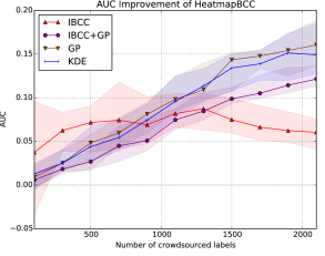
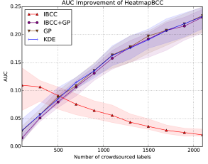
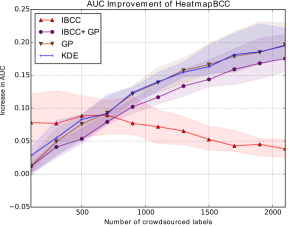
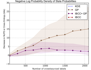
Figure 1: Synthetic data, noisy reporters: median improvement of HeatmapBCC over alternatives over 25 datasets, against number of crowdsourced labels. Shaded areas show inter-quartile range. Top-left: AUC, 25% noisy reporters. Top-right: AUC, 50% noisy reporters. Bottom-left: AUC, 75% noisy reporters. Bottom-right: NLPD of state probabilities, $\boldsymbol{\rho}$, with 50% noisy reporters.

Noisy reporters: the first experiment tests robustness to error-prone annotators. For each of the $25$ ground truth datasets, we generated three crowds of $20$ reporters. In each crowd, we varied the number of reliable reporters between $5$, $10$ and $15$, while the remainder were noisy reporters with high random error rates. We simulated reliable reporters by drawing confusion matrices, $\boldsymbol{\pi}^{(s)}$, from beta distributions with parameter matrix set to $\boldsymbol{\alpha}^{(s)}_{jj}=10$ along the diagonals and $1$ elsewhere. For noisy workers, all parameters were set equally to $\boldsymbol{\alpha}^{(s)}_{jl}=5$. For each proportion of noisy reporters, we selected reporters and grid points at random, and generated $2400$ reports by drawing binary labels from the confusion matrices $\boldsymbol{\pi}^{(1)},...,\boldsymbol{\pi}^{(20)}$. We ran the incremental train/test procedure for each crowd with each of the $25$ ground truth datasets. For HeatmapBCC, GP and IBCC+GP the kernel hyperparameters were set as $l=20$, $a_{0}=1$, and $b_{0}=1$. For HeatmapBCC, IBCC and IBCC+GP, we set confusion matrix hyperparameters to $\boldsymbol{\alpha}^{(s)}_{j,j}=2$ along the diagonals and $\boldsymbol{\alpha}^{(s)}_{j,l}=1$ elsewhere, assuming a weak tendency toward correct labels. For IBCC we also set $\nu_{0}=[1,1]$.

Figure 1 shows the median differences in AUC between HeatmapBCC and the alternative methods for noisy reporters. Plotting the difference between methods allows us to see consistent performance differences when AUC varies substantially between runs. More reliable workers increase the AUC improvement of HeatmapBCC. With all proportions of workers, the performance improvements are smaller with very small numbers of labels, except against IBCC, as none of the methods produce a confident model with very sparse data. As more labels are gathered, there are more locations with multiple reports, and IBCC is able to make good predictions at those points, thereby reducing the difference in AUC as the number of labels increases. However, for the other three methods, the difference in AUC continues to increase, as they improve more slowly as more labels are received. With more than 700 labels, using the GP to estimate the class labels directly is less effective than using IBCC classifications at points where we have received reports, hence the poorer performance of GP and IBCC+GP.

In Figure 1 we also show the improvement in negative log probability density (NLPD) of state probabilities, $\boldsymbol{\rho}$. We compare HeatmapBCC only against the methods that place a posterior distribution over their estimated state probabilities. As more labels are received, the IBCC+GP method begins to improve slightly, as it is begins to identify the noisy reporters in the crowd. The GP is much slower to improve due to the presence of these noisy labels.

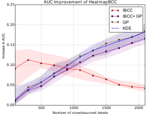
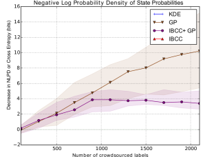
Figure 2: Synthetic data, 50% biased reporters: median improvement of HeatmapBCC compared to alternatives over 25 datasets, against number of crowdsourced labels. Shaded areas showing the inter-quartile range. Left: AUC. Right: NLPD of state probabilities, $\boldsymbol{\rho}$.

Biased reporters: the second experiment simulates the scenario where some reporters choose the negative class label overly frequently, e.g. because they fail to observe the positive state when it is present. We repeated the procedure used for noisy reporters but replaced the noisy reporters with biased reporters generated using the parameter matrix $\boldsymbol{\alpha}^{(s)}=\left[\begin{smallmatrix}7&1\\ 6&2\end{smallmatrix}\right]$. We observe similar performance improvements to the first experiment with noisy reporters, as shown in Figure 2, suggesting that HeatmapBCC is also better able to model biased reporters from sparse data than rival approaches.

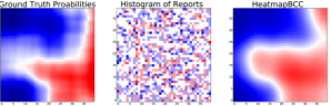
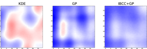
Figure 3: Synthetic data, 50% biased reporters: posterior distributions. Histogram of reports shows the difference between positive and negative label frequencies at each grid square.

Figure 3 shows an example of the posterior distributions over $t_{\boldsymbol{x}}$ produced by each method when trained on $1500$ random labels from a simulated crowd with $50\%$ biased reporters. We can see that the ground truth appears most similar to the HeatmapBCC estimates, while IBCC is unable to perform any smoothing.

Continuous report locations: in the previous experiments we drew reports from discrete grid points so that multiple reporters produced noisy labels for the same target, $t_{\boldsymbol{x}}$. The third experiment tests the behaviour of our model with reports drawn from continuous locations, with 50% noisy reporters drawn as in the first experiment. In this case, our model receives only one report for each object $t_{\boldsymbol{x}}$ at the input locations $\boldsymbol{X}$. Figure 4 shows that the difference in AUC between HeatmapBCC and other methods is significantly reduced, although still positive. This may be because we are reliant on $\rho$ to make classifications, since we have not observed any reports for the exact test locations $\boldsymbol{X}^{*}$. If $\rho_{\boldsymbol{x}}$ is close to $0.5$, the prediction for class label $\boldsymbol{x}$ is uncertain. However, the improvement in NLPD of the state probabilities $\boldsymbol{\rho}$ is less affected by using continuous locations, as seen by comparing Figure 1 with Figure 4, suggesting that HeatmapBCC remains advantageous when there is only one report at each training location. In practice, reports at neighbouring locations may be intended to refer to the same $t_{\boldsymbol{x}}$, so if reports are treated as all relating to separate objects, they could bias the state probabilities. Grouping reports into discrete grid squares avoids this problem and means we obtain a state classification for each square in the heatmap. We therefore continue to use discrete grid locations in our real-world experiments.

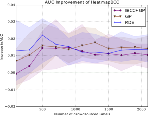
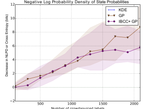
Figure 4: Synthetic data, 50% noisy reporters, continuous report locations. Median improvement of HeatmapBCC compared to alternatives over 25 datasets, against number of crowdsourced labels. Shaded areas showing the inter-quartile range. Left: AUC. Right: NLPD of state probabilities, $\boldsymbol{\rho}$.

4.2 Crowdsourced Labels of Satellite Images

We obtained a set of 5,477 crowdsourced labels from a trial run of the Zooniverse Planetary Response Network project. In this application, volunteers labelled satellite images showing damage to Tacloban, Philippines, after Typhoon Haiyan/Yolanda. The volunteers’ task was to mark features such as damaged buildings, blocked roads and floods. For this experiment, we first divided the area into a $132\times 92$ grid. The goal was then to combine crowdsourced labels to classify grid squares according to whether they contain buildings with major damage or not. We treated cases where a user observed an image but did not mark any features as a set of multiple negative labels, one for each of the grid squares covered by the image. Our dataset contained 1,641 labels marking buildings with major structural damage, and 1,245 negative labels. Although this dataset does not contain ground truth annotations, it contains enough crowdsourced annotations that we can confidently determine labels for most of the region of interest using all data. The aim is to test whether our approach can replicate these results using only a subset of crowdsourced labels, thereby reducing the workload of the crowd by allowing for sparser annotations. We therefore defined gold-standard labels by running IBCC on the complete set of crowdsourced labels, and then extracting the IBCC posterior probabilities for $572$ data points with $\geq 3$ crowdsourced labels where the posterior of the most probable class $\geq 0.9$. The IBCC hyperparameters were set to $\boldsymbol{\alpha}^{(s)}_{0,j,j}=2$ along the diagonals, $\boldsymbol{\alpha}_{0,j,l}^{(s)}=1$ elsewhere, and $\nu_{0}=[100,100]$.

We ran our incremental train/test procedure 20 times with initial subsets of 178 random labels. Each of these 20 repeats required approximately 45 minutes runtime on an Intel i7 desktop computer. The length-scales $l$ for HeatmapBCC, GP and IBCC+GP were optimised at each iteration using maximum likelihood II by maximising the variational lower bound on the log likelihood (Equation 11), as described in [16]. The inverse scale hyperparameters were set to $a_{0}=0.5$ and $b_{0}=5$, and the other hyperparameters were set as for gold label generation. We did not find a significant difference when varying diagonal confusion matrix values $\boldsymbol{\alpha}^{(s)}_{j,j}=2$ from $2$ to $20$.

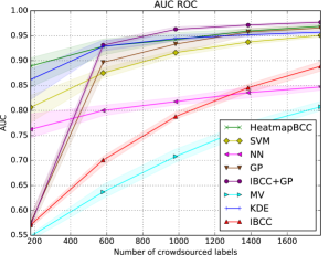
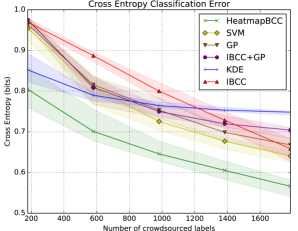
Figure 5: Planetary Response Network, major structural damage data. Median values over 20 repeats against the number of randomly selected crowdsourced labels. Shaded areas show the inter-quartile range. Left: AUC. Right: cross entropy error.

In Figure 5 (left) we can see how AUC varies as more labels are introduced, with HeatmapBCC, GP and IBCC+GP converging close to our gold-standard solution. HeatmapBCC performs best initially, potentially because it can learn a more suitable length-scale with less data than GP and IBCC+GP. SVM outperforms GP and IBCC+GP with $178$ labels, but is outperformed when more labels are provided. Majority voting, nearest neighbour and IBCC produce much lower AUCs than the other approaches. The benefits of HeatmapBCC can be more clearly seen in Figure 5 (right), which shows a substantial reduction in cross entropy classification error compared to alternative methods, indicating that HeatmapBCC produces better probability estimates.

4.3 Haiti Earthquake Text Messages

Here we aggregate text reports written by members of the public after the Haiti 2010 Earthquake. The dataset we use was collected and labelled by Ushahidi[14]. We have selected 2,723 geo-tagged reports that were sent mainly by SMS and were categorised by Ushahidi volunteers. The category labels describe the type of situation that is reported, such as “medical emergency" or “collapsed building". In this experiment, we aim to predict a binary class label, "emergency" or "no emergency" by combining all reports. We model each category as a different information source; if a category label is present for a particular message, we observe a value of $1$ from that information source at the message’s geo-location. This application differs from the satellite labelling task because many of the reports do not explicitly report emergencies and may be irrelevant. In the absence of ground truth data, we establish a gold-standard test set by training IBCC on all 2723 reports, placed into 675 discrete locations on a $100\times 100$ grid. Each grid square has approximately 4 reports. We set IBCC hyper-parameters to $\boldsymbol{\alpha}^{(s)}_{0,j,j}=100$ along the diagonals, $\boldsymbol{\alpha}^{(s)}_{0,j,l}=1$ elsewhere, and $\boldsymbol{\nu}_{0}=[2000,1000]$.

Since the Ushahidi data set contains only reports of emergencies, and does not contain reports stating that no emergency is taking place, we cannot learn the length-scale $l$ from this data, and must rely on background knowledge. We therefore select another dataset from the Haiti 2010 Earthquake, which has gold standard labels, namely the building damage assessment provided by UNOSAT [2]. We expect this data to have a similar length-scale because the underlying cause of both the building damages and medical emergencies was an earthquake affecting built-up areas where people were present. We estimated $l$ using maximum likelihood II optimisation, giving an optimal value of $l=16$ grid squares. We then transferred this point estimate to the model of the Ushahidi data. Our experiment repeated the incremental train/test procedure 20 times with hyperparameters set to $a_{0}=1500$, $b_{0}=1500$, $\boldsymbol{\alpha}^{(s)}_{0,j,j}=100$ along the diagonals, $\boldsymbol{\alpha}^{(s)}_{0,j,l}=1$ elsewhere, and $\boldsymbol{\nu}_{0}=[2000,1000]$.

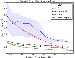
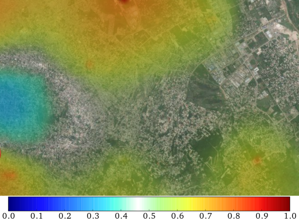
Figure 6: Haiti text messages. Left: cross entropy error against the number of randomly selected crowdsourced labels. Lines show the median over 25 repeats, with shaded areas showing the inter-quartile range. Gold standard defined by running IBCC with 675 labels using a $100\times 100$ grid. Right: heatmap of emergencies for part of Port-au-Prince after the 2010 Earthquake, showing high probability (dark orange) to low probability (blue).

Figure 6 shows that HeatmapBCC is able to achieve low error rates when the reports are sparse. The IBCC and HeatmapBCC results do not quite converge due to the effect of interpolation performed by HeatmapBCC, which can still affect the results with several reports per grid square. The gold-standard predictions from IBCC also contain some uncertainty, so cross entropy does not reach zero, even with all labels. The GP alone is unable to determine the different reliability levels of each report type, so while it is able to interpolate between sparse reports, HeatmapBCC and IBCC detect the reliable data and produce different predictions when more labels are supplied. In summary, HeatmapBCC produces predictions with 439 labels (65%) that has an AUC within 0.1 of the gold standard predictions produced using all 675 labels, and reduces cross entropy to 0.1 bits with 400 labels (59%), showing that it is effective at predicting emergency states with reduced numbers of Ushahidi reports. Using an Intel i7 laptop, the HeatmapBCC inference over 675 labels required approximately one minute.

We use HeatmapBCC to visualise emergencies in Port-au-Prince, Haiti after the 2010 earthquake, by plotting the posterior class probabilities as the heatmap shown in Figure 6. Our example shows how HeatmapBCC can combine reports from trusted sources with crowdsourced information. The blue area shows a negative report from a simulated first responder, with confusion matrix hyperparameters set to $\boldsymbol{\alpha}^{(s)}_{0,j,j}=450$ along the diagonals, so that the negative report was highly trusted and had a stronger effect than the many surrounding positive reports. Uncertainty in the latent function $f_{j}$ can be used to identify regions where information is lacking and further reconnaisance is necessary. Probabilistic heatmaps therefore offer a powerful tool for situation awareness and planning in disaster response.

5 Conclusions

In this paper we presented a novel Bayesian approach to aggregating unreliable discrete observations from different sources to classify the state across a region of space or time. We showed how this method can be used to combine noisy, biased and sparse reports and interpolate between them to produce probabilistic spatial heatmaps for applications such as situation awareness. Our experiments demonstrated the advantages of integrating a confusion matrix model to capture the unreliability of different information sources with sharing information between sparse report locations using Gaussian processes. In future work we intend to improve scalability of the GP using stochastic variational inference [6] and investigate clustering confusion matrices using a hierarchical prior, as per [13, 23], which may improve the ability to learn confusion matrices when data for individual information sources is sparse.

References

- [1] Adams, R.P., Murray, I., MacKay, D.J.: Tractable nonparametric bayesian inference in poisson processes with gaussian process intensities. In: Proceedings of the 26th Annual International Conference on Machine Learning. pp. 9–16. ACM (2009)
- [2] Corbane, C., Saito, K., Dell’Oro, L., Bjorgo, E., Gill, S.P., Emmanuel Piard, B., Huyck, C.K., Kemper, T., Lemoine, G., Spence, R.J., et al.: A comprehensive analysis of building damage in the 12 january 2010 Mw7 Haiti earthquake using high-resolution satellite and aerial imagery. Photogrammetric Engineering & Remote Sensing 77(10), 997–1009 (2011)
- [3] Dawid, A.P., Skene, A.M.: Maximum likelihood estimation of observer error-rates using the EM algorithm. Journal of the Royal Statistical Society. Series C (Applied Statistics) 28(1), 20–28 (Jan 1979)
- [4] Felt, P., Ringger, E.K., Seppi, K.D.: Semantic annotation aggregation with conditional crowdsourcing models and word embeddings. In: International Conference on Computational Linguistics. pp. 1787–1796 (2016)
- [5] Girolami, M., Rogers, S.: Variational Bayesian multinomial probit regression with Gaussian process priors. Neural Computation 18(8), 1790–1817 (2006)
- [6] Hensman, J., Matthews, A.G.d.G., Ghahramani, Z.: Scalable variational Gaussian process classification. In: International Conference on Artificial Intelligence and Statistics (2015)
- [7] Kim, H., Ghahramani, Z.: Bayesian classifier combination. Gatsby Computational Neuroscience Unit Technical Report GCNU-T.,London, UK (2003)
- [8] Kom Samo, Y.L., Roberts, S.J.: Scalable nonparametric Bayesian inference on point processes with Gaussian processes. In: International Conference on Machine Learning. pp. 2227–2236 (2015)
- [9] Kottas, A., Sansó, B.: Bayesian mixture modeling for spatial poisson process intensities, with applications to extreme value analysis. Journal of Statistical Planning and Inference 137(10), 3151–3163 (2007)
- [10] Lintott, C.J., Schawinski, K., Slosar, A., Land, K., Bamford, S., Thomas, D., Raddick, M.J., Nichol, R.C., Szalay, A., Andreescu, D., et al.: Galaxy zoo: morphologies derived from visual inspection of galaxies from the sloan digital sky survey. Monthly Notices of the Royal Astronomical Society 389(3), 1179–1189 (2008)
- [11] Long, C., Hua, G., Kapoor, A.: A joint Gaussian process model for active visual recognition with expertise estimation in crowdsourcing. International Journal of Computer Vision 116(2), 136–160 (2016)
- [12] Meng, C., Jiang, W., Li, Y., Gao, J., Su, L., Ding, H., Cheng, Y.: Truth discovery on crowd sensing of correlated entities. In: 13th ACM Conference on Embedded Networked Sensor Systems. pp. 169–182. ACM (2015)
- [13] Moreno, P.G., Teh, Y.W., Perez-Cruz, F.: Bayesian nonparametric crowdsourcing. Journal of Machine Learning Research 16, 1607–1627 (2015)
- [14] Morrow, N., Mock, N., Papendieck, A., Kocmich, N.: Independent Evaluation of the Ushahidi Haiti Project. Development Information Systems International 8, 2011 (2011)
- [15] Parzen, E.: On estimation of a probability density function and mode. The annals of mathematical statistics 33(3), 1065–1076 (1962)
- [16] Rasmussen, C.E., Williams, C.K.I.: Gaussian processes for machine learning. The MIT Press, Cambridge, MA, USA 38, 715–719 (2006)
- [17] Raykar, V.C., Yu, S.: Eliminating spammers and ranking annotators for crowdsourced labeling tasks. Journal of Machine Learning Research 13, 491–518 (2012)
- [18] Reece, S., Roberts, S., Nicholson, D., Lloyd, C.: Determining intent using hard/soft data and gaussian process classifiers. In: 14th International Conference on Information Fusion. pp. 1–8. IEEE (2011)
- [19] Rosenblatt, M., et al.: Remarks on some nonparametric estimates of a density function. The Annals of Mathematical Statistics 27(3), 832–837 (1956)
- [20] Simpson, E., Roberts, S., Psorakis, I., Smith, A.: Dynamic Bayesian combination of multiple imperfect classifiers. Intelligent Systems Reference Library series Decision Making with Imperfect Decision Makers, 1–35 (2013)
- [21] Simpson, E.D., Venanzi, M., Reece, S., Kohli, P., Guiver, J., Roberts, S.J., Jennings, N.R.: Language understanding in the wild: Combining crowdsourcing and machine learning. In: 24th International Conference on World Wide Web. pp. 992–1002 (2015)
- [22] Steinberg, D.M., Bonilla, E.V.: Extended and unscented gaussian processes. In: Advances in Neural Information Processing Systems. pp. 1251–1259 (2014)
- [23] Venanzi, M., Guiver, J., Kazai, G., Kohli, P., Shokouhi, M.: Community-based bayesian aggregation models for crowdsourcing. In: 23rd international conference on World wide web. pp. 155–164 (2014)
- [24] Venanzi, M., Guiver, J., Kohli, P., Jennings, N.R.: Time-sensitive Bayesian information aggregation for crowdsourcing systems. Journal of Artificial Intelligence Research 56, 517–545 (2016)
- [25] Venanzi, M., Rogers, A., Jennings, N.R.: Crowdsourcing spatial phenomena using trust-based heteroskedastic Gaussian processes. In: 1st AAAI Conference on Human Computation and Crowdsourcing (HCOMP) (2013)