The large $N$ phase diagram of ${\cal N}=2$ $SU(N)$ Chern-Simons theory with one fundamental chiral multiplet

Abstract

We study the theory of a single fundamental fermion and boson coupled to Chern-Simons theory at leading order in the large $N$ limit. Utilizing recent progress in understanding the Higgsed phase in Chern-Simons-Matter theories, we compute the quantum effective potential that is exact to all orders in the ’t Hooft coupling for the lightest scalar operator of this theory at finite temperature. Specializing to the zero temperature limit we use this potential to determine the phase diagram of the large $N$ ${\cal N}=2$ supersymmetric theory with this field content. This intricate two dimensional phase diagram has four topological phases that are separated by lines of first and second order phase transitions and includes special conformal points at which the infrared dynamics is governed by Chern-Simons theory coupled respectively to free bosons, Gross-Neveu fermions, and to a theory of Wilson-Fisher bosons plus free fermions. We also describe the vacuum structure of the most general $\mathcal{N}=1$ supersymmetric theory with one fundamental boson and one fundamental fermion coupled to an $SU(N)$ Chern-Simons gauge field, at arbitrary values of the ’t Hooft coupling.

1 Introduction

In this paper we continue the study, initiated in Jain:2013gza ; Gur-Ari:2015pca ; Aharony:2018pjn , of $U(N)$ (or $SU(N)$) Chern-Simons theories coupled to a single fundamental boson $\phi$ and a single fundamental fermion $\psi$ in the large $N$ limit. The theory we study is governed by the most general ‘power counting renormalizable’ Lagrangian

$$S =\int d^{3}x\biggl{[}\frac{i\kappa}{4\pi}\epsilon^{\mu\nu\rho}\mathrm{Tr}(X_{\mu}\partial_{\nu}X_{\rho}-\tfrac{2i}{3}X_{\mu}X_{\nu}X_{\rho})$$

$$+\overline{D_{\mu}\phi}D^{\mu}\phi+\bar{\psi}\gamma^{\mu}D_{\mu}\psi+m_{B}^{2}\bar{\phi}\phi+m_{F}\bar{\psi}\psi+\frac{4\pi b_{4}}{\kappa}(\bar{\phi}\phi)^{2}+\frac{4\pi^{2}(x_{6}+1)}{\kappa^{2}}(\bar{\phi}\phi)^{3}$$

$$+\frac{4\pi x_{4}}{\kappa}(\bar{\psi}\psi)(\bar{\phi}\phi)+\frac{2\pi(y_{4}^{\prime}-3)}{\kappa}(\bar{\psi}\phi)(\bar{\phi}\psi)+\frac{2\pi y_{4}^{\prime\prime}}{\kappa}\left((\bar{\psi}\phi)(\bar{\psi}\phi)+(\bar{\phi}\psi)(\bar{\phi}\psi)\right)\biggl{]}\ ,$$ (1)

. The theories (1) are of interest partly because they have been conjectured Jain:2013gza ; Gur-Ari:2015pca to enjoy invariance under a level-rank type strong-weak coupling duality under which fermions are interchanged with bosons. In the large $N$ ’t Hooft limit

$$\kappa\to\infty\ ,\quad N\to\infty\ ,\quad\lambda=\frac{N}{\kappa}\quad\text{held fixed}\ ,$$ (2)

within which we work in this paper, the parameters of the theory transform under the duality according to

$$N^{\prime}=|\kappa|-N\ ,\quad\kappa^{\prime}=-\kappa\ ,\quad\lambda^{\prime}=\lambda-\text{sgn}(\lambda)\ ,$$

$$x_{4}^{\prime}=\frac{1}{x_{4}}\ ,\quad x_{6}^{\prime}=-\frac{x_{6}}{x_{4}^{3}}\ ,\quad(y_{4}^{\prime})^{\prime}=\frac{16y_{4}^{\prime}}{y_{4}^{\prime 2}-4y_{4}^{\prime\prime 2}}\ ,\quad(y_{4}^{\prime\prime})^{\prime}=-\frac{16y_{4}^{\prime\prime}}{y_{4}^{\prime 2}-4y_{4}^{\prime\prime 2}}\ ,$$

$$b_{4}^{\prime}=-\frac{b_{4}}{x_{4}^{2}}+\frac{3}{4}\frac{x_{6}}{x_{4}^{3}}m_{F}\ ,\quad m_{B}^{\prime 2}=-\frac{1}{x_{4}}m_{B}^{2}-\frac{3}{4}\frac{x_{6}}{x_{4}^{3}}m_{F}^{2}+\frac{2}{x_{4}^{2}}b_{4}m_{F}\ ,\quad m_{F}^{\prime}=-\frac{m_{F}}{x_{4}}\ .$$ (3)

as derived in Jain:2013gza ; Gur-Ari:2015pca . This duality is a generalisation of the recently much-studied dualities between purely fermionic and purely bosonic Chern-Simons matter theories Jain:2013gza -Cordova:2017vab , and turn out (see below, generalising Jain:2013gza ; Aharony:2018pjn ) to imply these earlier dualities in special scaling limits.

There is another angle from which one may view the dualities (1). Note that the theory (1) is ${\cal N}=2$ superconformal when

$$m_{F}=m_{B}^{2}=b_{4}=0\ ,\quad x_{4}=1\ ,\quad x_{6}=0\ ,\quad y_{4}^{\prime}=4\ ,\quad y_{4}^{\prime\prime}=0\ .$$ (4)

(the transformations in (1) leaves (4) invariant). It follows that the dualities of (1) may also be viewed as a generalisation of the Giveon-Kutasov type supersymmetric duality of the $\mathcal{N}=2$ theory. The study of the theories (1) thus seems particularly interesting, as it holds the possibility of tying together two rich but largely independent streams of work (so far), namely the large $N$ studies of (non-supersymmetric in general) Chern-Simons-Matter theories and the exact finite $N$ studies of supersymmetric Chern-Simons-Matter theories.

In this paper we calculate an exact (i.e. all orders in the ’t Hooft coupling $\lambda$) analytic expression for the finite temperature quantum effective potential for the lightest gauge invariant scalar - ${\bar{\phi}\phi}$ - of the theory (1). In fact, we give a five-variable off-shell free energy for the theory (1) at finite temperature in Section 2, which, upon integrating out four of the five variables, results in the aforementioned quantum effective potential. The precise relation between our off-shell free energy and the quantum effective potential is described in Section 2.4.

The computations presented in this paper can be motivated by the following observation. Setting all kinetic and fermion terms to zero, the action (1) reduces to a cubic potential in the variable $\xi=\frac{2\pi{\bar{\phi}}\phi}{\kappa}$:

$$U_{\rm cl}(\xi)=2\pi\kappa\left(m_{B}^{2}\xi+2b_{4}\xi^{2}+(x_{6}+1)\xi^{3}\right)\ \ .$$ (5)

Note that $\kappa\,\xi>0$ classically. Clearly this classical potential is then bounded from below if and only if

$$x_{6}>-1\ .$$ (6)

In analogy with its classical counterpart, the quantum theory will also be unstable to decay to $\kappa\,\xi\to\infty$ - and so will be ill-defined - when $x_{6}$ is sufficiently negative. One of the goals of this paper is to determine the (all orders in $\lambda$) quantum version of the stability condition (6). In order to accomplish this we evaluate the exact quantum effective potential for the variable

$$\sigma=\frac{\xi}{\lambda}=\frac{2\pi\bar{\phi}\phi}{N}\ ,$$ (7)

(i.e. a quantum effective potential for the lightest gauge-invariant scalar operator $\bar{\phi}\phi$) and work out the condition that ensures that this effective potential is bounded from below at large $\sigma$.

Our result for the exact quantum effective potential for the variable $\sigma$ defined in (7) has a surprise. Quantum mechanically $\sigma$ is not necessarily positive definite (the subtraction needed to define the composite operator ${\bar{\phi}}\phi$ could be negative). As a consequence, we shall see that the quantum effective potential for $\sigma$ is well-defined also for negative $\sigma$, apart from being well-defined for positive $\sigma$. The detailed form of the quantum effective potential is listed in (2) at finite temperature and in (45) at zero temperature.

Thus, there will be two conditions for our theory to be stable: firstly, a quantum-corrected version of (6) which arises from requiring the quantum effective potential to be bounded from below for large and positive $\sigma$; a second condition from the requirement that the quantum effective potential must be bounded from below at large negative $\sigma$ as well. As in the recent paper Dey:2018ykx , this second condition - which has no classical counterpart - results in a second inequality for the variable $x_{6}$. This inequality defines an upper bound for $x_{6}$ and hence it is necessary for the stability of the theory that $x_{6}$ is smaller than a minimum value. It follows that the theory (1) is well-defined if and only if $x_{6}$ lies within an interval of values. The lower and upper limits of this interval turn out to depend on $x_{4}$ as well as the ’t Hooft coupling $\lambda$ and are listed in detail in equation (3) of Section 3 below.

Of course the large $N$ exact quantum effective potential computed in this paper has many applications beyond the analysis of vacuum stability. For instance, we demonstrate in Section 2.1 that the quantum effective potential presented in this paper enjoys invariance under the conjectured strong-weak coupling duality (1), yielding nontrivial new evidence for this duality (generalising earlier results of Jain:2013gza ; Aharony:2018pjn ).

However, the principal results of this paper concern the use of the quantum effective potential to quantitatively (and exactly at large $N$) determine the zero-temperature phase diagram of the theories (1). We obtain this phase diagram by minimising the quantum effective potential - which turns out to be piecewise cubic at zero temperature - as a function of the parameters of (1) - and thereby determining the dominant phase of our theory at zero temperature.

The theory (1) has four dimensionless parameters ($x_{6}$, $x_{4}$, $y_{4}^{\prime}$, $y_{4}^{\prime\prime}$) and three dimensionful parameters $m_{B}^{2},m_{F}$ and $b_{4}$ (and so two additional dimensionless ratios). By varying these six parameters we could, in principle, obtain a six dimensional phase diagram. In this paper we do not explore the full six dimensional phase diagram but study only two relatively simple slices of it. The first of these is the ‘phase diagram of the large $N$ ${\cal N}=2$ theory’ (see below for an explanation of these words), i.e. the phase diagram obtained by setting the four dimensionless parameters $x_{4},x_{6},y_{4}^{\prime},y_{4}^{\prime\prime}$ to the values (4) but allowing the dimensionful variables $m_{B}^{2},b_{4},m_{F}$ in (1) to be arbitrary. Trading one of the dimensionful parameters for a mass scale, the phase diagram thus obtained is two dimensional. The second slice we study is obtained by restricting our attention to the class of theories in (1) that preserve at least ${\cal N}=1$ supersymmetry:

$$m_{F}=\mu\ ,\ \ m_{B}^{2}=\mu^{2}\ ,\ \ b_{4}=\mu w\ ,\quad x_{4}=\frac{1+w}{2}\ ,\quad x_{6}=w^{2}-1\ ,\quad y_{4}^{\prime}=3+w\ ,\quad y_{4}^{\prime\prime}=w-1\ .$$ (8)

There is one dimensionful parameter $\mu$ on this slice which can be traded for a mass scale and the remaining one dimensionless parameter $w$ describes the one dimensional phase diagram.

Our motivation for studying special slices of (1) - rather than the whole shebang at once - are both practical as well as conceptual in nature. At the practical level, a two (or one) dimensional phase space is much easier to visualise than a six dimensional phase space. The conceptual reason is more important, and we pause, over the next three paragraphs, to give provide a detailed explanation.

Recall that a quantum field theory is defined in the UV as a fixed point of the renormalization group. The phase diagram of a given quantum field theory is defined as the set of phases obtained by deforming the particular fixed point of interest with all possible relevant deformations. In order to understand the phase diagram of particular theories of the form (1) we need to first identify the set of fixed points (in the space of RG flows of the four dimensionless couplings in (1)). With this understanding in hand we can then study the phase diagram of any given fixed point.

The study of fixed points of the Lagrangian (1) is complicated by the following fact; the beta function for all dimensionless parameters in (1) vanishes in the strict large $N$ limit. At leading order in large $N$ it follows that the Lagrangian (1) describes a four dimensional hyperplane of conformal field theories rather than the more usual situation of a collection of isolated fixed points. This picture is, of course, an artefact of the large $N$ limit. At any finite $N$, no matter how large, this fixed hyperplane presumably breaks up into a set of isolated fixed points connected by a presumably intricate pattern of RG flows. Each of these fixed points defines a new conformal field theory; the phase diagram of this theory is obtained by studying its relevant deformations.

It follows that there are as many physically interesting phase diagram questions in (1) as there are fixed points under the RG flow (of the dimensionless variables) of (1). Unfortunately the aforementioned RG flows have not yet been studied, and their fixed points have not yet been classified. Despite this general state of ignorance, we do know of one fixed point for the class of theories (1). This is the ${\cal N}=2$ supersymmetric point defined by (4) which lies on the fixed hyperplane of the RG flow at leading order in the large $N$ limit. It also seems likely that deformations about this point that are tangent to the four dimensional fixed hyperplane are actually irrelevant once subleading corrections in $1/N$ are taken into account. Assuming this to be the case, it follows that the phase diagram associated with this special fixed point - i.e. the phase diagram of the ${\cal N}=2$ theory - is obtained at large $N$ by restricting attention to the special point (4) in the manifold of parameters.

Returning to the main flow of this introduction, the phase diagram of the ${\cal N}=2$ supersymmetric theory is parametrized by two dimensionless numbers that live on a space with the topology of a sphere, and turns out to be rather intricate. A major part of this phase diagram consists of regions of four distinct massive (more precisely, topological) phases. The long distance dynamics of these phases is governed by pure Chern-Simons theories with gauge group either $SU(N)$ or $SU(N-1)$; the rank is $N$ or $N-1$ depending on whether the massive bosons are unHiggsed or Higgsed. We denote these as the $+$ and $-$ phases respectively of the boson. The level of the low energy topological Chern-Simons theory is either $k$ or $k-\text{sgn}(k)$ depending on whether the dynamical massive fermions that we integrate out to obtain the topological theory have the same sign or opposite sign w.r.t. $k$. These we term as the $+$ and $-$ phases of the fermion. The four massive phases are then described by one sign for the phase of the boson and one sign for the phase of the fermion. In the rest of this paper we use the notation explained in Table 1 for these four massive phases of our theory.

Phase	Fermion	Boson	Low-energy TQFT
$(+,+)$	$\text{sgn}({\tilde{m}}_{F})=\text{sgn}(k)$	unHiggsed	$SU(N)_{k}$
$(-,+)$	$\text{sgn}({\tilde{m}}_{F})=-\text{sgn}(k)$	unHiggsed	$SU(N)_{k-\text{sgn}(k)}$
$(+,-)$	$\text{sgn}({\tilde{m}}_{F})=\text{sgn}(k)$	Higgsed	$SU(N-1)_{k}$
$(-,-)$	$\text{sgn}({\tilde{m}}_{F})=-\text{sgn}(k)$	Higgsed	$SU(N-1)_{k-\text{sgn}(k)}$

Table 1: The four massive phases of the one boson-one fermion theory. The notation is $(F,B)$ with $F$ and $B$ being the fermionic and bosonic phases respectively. The effective fermion mass is denoted by ${\tilde{m}}_{F}$ and $\text{sgn}({\tilde{m}}_{F})$ and $\text{sgn}(k)$ are the signs of ${\tilde{m}}_{F}$ and $k$ respectively. We list the Chern-Simons TQFTs as appropriate for an $SU(N)$ gauge group for the microscopic theory.

The phase diagram of the ${\cal N}=2$ theory turns out to be qualitatively different depending on whether the absolute value $|\lambda|$ of ’t Hooft coupling is less than or greater than half. The schematic phase diagram in each case is sketched in Figure 1 (see Figures 15,16,17 for the actual accurate phase diagram at three sample values of $\lambda$). Notice that the regions of the four topological phases above are separated by blue or green lines. These are lines along which the theory undergoes a second order or a first order transition respectively. Along the second order phase transition lines the dynamics is conformal and is generically governed by either the critical boson (CB) or the regular fermion (RF) theories. At one point on one of these phase transition lines, the order of the phase transition jumps from second to first order. At this transition point the theory reduces to the conformal Regular Boson (RB) theory (when $|\lambda|<\frac{1}{2}$) or the conformal Critical Fermion (CF) theory (when $|\lambda|>\frac{1}{2}$). Note also that in both cases there is a point on the phase diagram at which the four second order phase transition lines meet. At this point the dynamics is governed by Chern-Simons gauged Wilson-Fisher bosons and regular fermions (the CB-RF theory). This theory was first encountered (in the same context) in Jain:2013gza , and has recently been intensively studied in their own right at finite values of $N$ in Jensen:2017bjo ; Benini:2017aed .

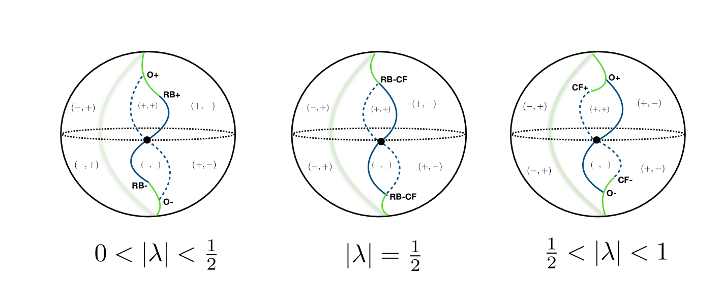
Figure 1: A schematic phase diagram for the $\mathcal{N}=2$ theory for three representative values of $|\lambda|$. The phase diagram is an ellipsoid (displayed here as a sphere for simplicity) in the three dimensional space spanned by the relevant parameters $m_{B}^{2}$, $\lambda b_{4}$ and $m_{F}\text{sgn}(\lambda)$. The northern (southern) hemisphere corresponds to $m_{F}\text{sgn}(\lambda)>0$ ($m_{F}\text{sgn}(\lambda)<0$) while the left (right) hemisphere corresponds to $m_{B}^{2}>0$ ($m_{B}^{2}<0$). The notation $(\pm,\pm)$ corresponds to the four low energy topological phases described in Table 1. The blue lines are second order transition lines and are governed by either CS gauged Wilson-Fisher bosons (solid lines) or CS gauged free fermions (dashed lines). The green line in each of the above figures is a first order phase transition line – part of it lies on the far side of the ellipsoid in the viewpoint depicted above. For $|\lambda|<\tfrac{1}{2}$ the first order line meets the solid blue lines at one point each in the two hemispheres of the ellipsoid governed by CS gauged free boson CFTs (${\rm RB}\pm$). For $|\lambda|>\tfrac{1}{2}$ these points are governed by CS gauged Gross-Neveu fermions (${\rm CF}\pm$). For $|\lambda|=\tfrac{1}{2}$, the first order line meets the solid and dashed lines at one point each in the two hemispheres which are governed by a theory of CS gauged free bosons plus Gross-Neveu fermions (RB-CF). The blue lines all intersect at the black dot on the equator and is governed by a theory of CS gauged Wilson-Fisher bosons plus free fermions (CB-RF). The phase diagrams for $|\lambda|<\tfrac{1}{2}$ and $|\lambda|>\tfrac{1}{2}$ are related to each other by the duality map (1). The diagram for $|\lambda|=\tfrac{1}{2}$ is self-dual.

Note also that the phase diagram at $|\lambda|=\frac{1}{2}$ has a qualitatively new feature; in each of the northern and the southern hemispheres this phase diagram has a special critical point that marks the simultaneous end point of both the second order CS-gauged Wilson-Fisher and CS-gauged free fermion phase transition lines. We present a brief qualitative discussion about this interesting sounding critical theory (and a related theory obtained by orbifolding this theory by its duality symmetry) at the end of Section 4.5.

In addition to our analysis of the phase structure of the ${\cal N}=2$ theory, in Section 5 we have also presented a separate analysis of the phase structure of the ${\cal N}=1$ subset of theories (8). Our final results are summarised in Figure 2.

Figure 2: The vacuum structure of the $\mathcal{N}=1$ theory (8) as a function of the parameter $w$. The two cases $\text{sgn}(\mu)=\pm\text{sgn}(\lambda)$ are given above and below the $w$ line respectively. The quantum effective potential either has one or two $\mathcal{N}=1$ supersymmetric vacua for a given range of $w$ and sign of $\mu\lambda$. In the cases where there are two such vacua, we have indicated both in the above phase diagram. The $w=1$ point corresponds to the $\mathcal{N}=2$ theory.

Recall that the distinct ${\cal N}=1$ theories (8) are labelled by a single dimensionless number $w$ and a dimensionful scale $\mu$. The phase diagram of our system depends on $w$ and ${\rm sgn}(\mu\lambda)$. In Figure 2 we present the phase of our system at all allowed values of $w$ and for both possible signs of $\mu\lambda$.

The results of Figure 2 overlap with those of Figure 1 in the special case $w=1$. When $\mu\lambda>0$, the ${\cal N}=1$ theory lies at a particular point in the $(+,+)$ region in the northern hemisphere of either of the diagrams in Figure 1. On the other hand when $\mu\lambda<0$ the ${\cal N}=1$ theory lies at a particular point on the southern hemisphere of either of the diagrams in Figure 1. Remarkably enough, the point in question turns out to lie exactly on the first order phase transition line between the $(+,-)$ and $(-,+)$ phases in the southern hemisphere. This explains why we have two possible phases - namely $(+,-)$ and $(-,+)$ - for the ${\cal N}=1$ theory at $w=1$.

We emphasize that, at the conceptual level, the results of Figure 2 are only physical at those values of $w$ at which the beta function has fixed points. While we know this is the case at $w=1$ (i.e. the ${\cal N}=2$ fixed point) we do not currently know other values of $w$ where such fixed points occur. Precisely this question is the subject of investigation of the soon to appear paper ofer .

Before ending this introduction we should emphasize that the finite temperature free energy of the same theory (1) was already computed in Jain:2013gza for the special case of the $(+,+)$ and $(-,+)$ phases. About half of the phase diagram presented in Figure 1 (i.e. the parts of the phase diagram covered by the $(+,+)$ and $(-,+)$ phases) could already have been constructed using the results of Jain:2013gza . The analysis of the phase diagram of the theory presented in this paper has two advantages over the approach of Jain:2013gza : one methodological and the second of principle. At the methodological level, the use of the simple quantum effective potential, as opposed to simply the value of the free energy at extrema (which is the only information we have access to using the methods of Jain:2013gza ), makes the analysis of the phase diagram more intuitive and much easier. The more important in-principle advantage of the approach of this paper is that the quantum effective potential allows us to access the $(+,-)$ and $(-,-)$ phases (the analysis of Jain:2013gza was blind to these phases) and thus allows us to compute the complete phase diagram schematically depicted in Figure 1, a task that could not have been accomplished using only the analysis of Jain:2013gza .

2 An off-shell free energy

As we have explained in the introduction, one of the principal technical results of this paper is an explicit formula for the off-shell finite temperature free energy, analytic in all its variables, for the class of field theories (1).

The off shell free energy presented in this paper is a close analogue of the ‘three-variable off-shell free energy’ for the regular boson theory presented in equation 4.2 of Dey:2018ykx . As in Dey:2018ykx , we obtain the thermodynamic finite temperature free energy of our system by extremizing the off-shell free energy w.r.t. its variables and choosing the dominant extremum. The derivation of the off-shell free energy for the theory (1) is a straightforward combination of the results and methods described in detail in Jain:2013gza ; Choudhury:2018iwf ; Dey:2018ykx . We relegate the derivation of this off-shell free energy to Appendix B. In this section we simply present our final answer.

The finite temperature off-shell free energy of the theory (1) is given by

$$F[c_{B},c_{F},{\tilde{{\cal S}}},{\tilde{{\cal C}}},\sigma]$$

$$=\frac{N}{6\pi}\bigg{[}-3{\hat{c}}_{B}^{2}{\hat{\sigma}}+\lambda^{2}{\hat{\sigma}}^{3}+3\left({\hat{m}}_{B}^{2}{\hat{\sigma}}+2\lambda{\hat{b}}_{4}{\hat{\sigma}}^{2}+(x_{6}+1)\lambda^{2}{\hat{\sigma}}^{3}\right)$$

$$\qquad\quad-4\lambda^{2}({\tilde{{\cal S}}}+{\hat{\sigma}})^{3}+6|\lambda|{\hat{c}}_{B}({\tilde{{\cal S}}}+{\hat{\sigma}})^{2}$$

$$\qquad\quad-{\hat{c}}_{B}^{3}+3\int_{-\pi}^{\pi}d\alpha\,\rho(\alpha)\,\int_{{\hat{c}}_{B}}^{\infty}dy\,y\,\left(\log\left(1-e^{-y-i\alpha}\right)+\log\left(1-e^{-y+i\alpha}\right)\right)$$

$$\qquad\quad-8\lambda^{2}{\tilde{{\cal C}}}^{3}-6\lambda{\tilde{{\cal C}}}^{2}{\hat{\tilde{m}}}_{F}-3{\tilde{{\cal C}}}\left({\hat{c}}_{F}^{2}-({\hat{\tilde{m}}}_{F}+2\lambda{\tilde{{\cal C}}})^{2}\right)$$

$$\qquad\quad+{\hat{c}}_{F}^{3}-3\int_{-\pi}^{\pi}d\alpha\,\rho(\alpha)\,\int_{{\hat{c}}_{F}}^{\infty}dy\,y\,\left(\log\left(1+e^{-y-i\alpha}\right)+\log\left(1+e^{-y+i\alpha}\right)\right)$$

$$\qquad\qquad\qquad\qquad\qquad\qquad\qquad\quad-\frac{1}{2\lambda}\frac{3{\hat{m}}_{F}(4{\hat{b}}_{4}{\hat{m}}_{F}x_{4}-4{\hat{m}}_{B}^{2}x_{4}^{2}-{\hat{m}}_{F}^{2}x_{6})}{8x_{4}^{3}}\Bigg{]}\ ,$$ (9)

where

$${\tilde{m}}_{F}=m_{F}+2x_{4}\lambda\sigma\ ,$$ (10)

and $\rho(\alpha)$ is the eigenvalue distribution function defined e.g. in equation (1.7) of Choudhury:2018iwf . The hats on the variables in (2) indicate that they have been scaled with appropriate powers of the temperature $T$ to make them dimensionless. Note that the large $N$ free energy does not depend on the dimensionless parameters $y_{4}^{\prime}$ and $y_{4}^{\prime\prime}$ in (1).

As we have mentioned on several occasions, (2) is a function of the five dynamical variables $c_{B}$, $c_{F}$, ${\tilde{\cal S}}$, ${\tilde{\cal C}}$ and $\sigma$ (in addition to the holonomy distribution $\rho(\alpha)$) and needs to be extremized w.r.t. these variables. After extremization (i.e. around any saddle point) these variables have the following physical interpretation:

1. $c_{B}$ and $c_{F}$ are the thermal masses of the bosonic and fermionic excitations respectively and are positive by definition.

2. ${\tilde{\cal C}}$ and ${\tilde{\cal S}}$ are related to appropriate moments ${\cal C}(c_{F})$ and ${\cal S}(c_{B})$ of the holonomy distribution $\rho(\alpha)$:

   $${\cal C}(c_{F}) =\frac{1}{2}\int_{-\pi}^{\pi}d\alpha\,\rho(\alpha)\left(\log(2\cosh(\tfrac{\hat{c}_{F}+i\alpha}{2}))+\log(2\cosh(\tfrac{\hat{c}_{F}-i\alpha}{2}))\right)\ ,$$

   $${\cal S}(c_{B}) =\frac{1}{2}\int_{-\pi}^{\pi}d\alpha\,\rho(\alpha)\left(\log(2\sinh(\tfrac{\hat{c}_{B}+i\alpha}{2}))+\log(2\sinh(\tfrac{\hat{c}_{B}-i\alpha}{2}))\right)\ .$$ (11)

3. The variable $\sigma$ is related to the expectation value of ${\bar{\phi}}\phi$ via

   $$\sigma=\frac{2\pi}{N}\langle{\bar{\phi}}\phi\rangle\ .$$ (12)

   See Section 5 of Dey:2018ykx for more details of this interpretation in the closely related context of the regular boson theory.

The last term of (2) is independent of all field variables; this term shifts the finite temperature free energy of our theory by a term proportional to $\frac{1}{T}$ and can be absorbed into a cosmological constant (equivalently vacuum energy) of the theory. We have added this ‘counterterm’ to (2) by hand; this particular choice has the virtue that it renders the full off-shell free energy invariant under the duality (1) (rather than duality invariant upto a shift of the cosmological constant counterterm). As we will show below the counterterm in fact vanishes when evaluated on supersymmetric vacua (and so agrees with the convention that assigns zero energy to susy vacua).

2.1 Duality invariance of the off-shell free energy

In this brief subsection we discuss the invariance of the off-shell free energy of the theory governed by the action (1) under the duality transformations (1). It is straightforward to check that the off-shell free energy (2) is invariant under the duality transformations (1):

$$N^{\prime}=|\kappa|-N\ ,\quad\kappa^{\prime}=-\kappa\ ,\quad\lambda^{\prime}=\lambda-\text{sgn}(\lambda)\ ,$$

$$x_{4}^{\prime}=\frac{1}{x_{4}}\ ,\quad x_{6}^{\prime}=-\frac{x_{6}}{x_{4}^{3}}\ ,\quad(y_{4}^{\prime})^{\prime}=\frac{16y_{4}^{\prime}}{y_{4}^{\prime 2}-4y_{4}^{\prime\prime 2}}\ ,\quad(y_{4}^{\prime\prime})^{\prime}=-\frac{16y_{4}^{\prime\prime}}{y_{4}^{\prime 2}-4y_{4}^{\prime\prime 2}}\ ,$$

$$b_{4}^{\prime}=-\frac{b_{4}}{x_{4}^{2}}+\frac{3}{4}\frac{x_{6}}{x_{4}^{3}}m_{F}\ ,\quad m_{B}^{\prime 2}=-\frac{1}{x_{4}}m_{B}^{2}-\frac{3}{4}\frac{x_{6}}{x_{4}^{3}}m_{F}^{2}+\frac{2}{x_{4}^{2}}b_{4}m_{F}\ ,\quad m_{F}^{\prime}=-\frac{m_{F}}{x_{4}}\ ,$$ (13)

provided the variables $c_{B}$, $c_{F}$, ${\tilde{{\cal S}}}$, ${\tilde{{\cal C}}}$ and $\sigma$ in (2) are redefined according to

$$c_{B}^{\prime}=c_{F}\ ,\quad c_{F}^{\prime}=c_{B}\ ,\quad\lambda^{\prime}{\tilde{\cal S}}^{\prime}=\frac{1}{2}\left(-\text{sgn}(\lambda)\hat{c}_{F}+2\lambda{\tilde{\cal C}}\right)\ ,$$

$$\lambda^{\prime}{\tilde{\cal C}}^{\prime}=\frac{1}{2}\left(-\text{sgn}(\lambda)\hat{c}_{B}+2\lambda\tilde{\cal S}\right)\ ,\quad\lambda^{\prime}\sigma^{\prime}=\frac{1}{2}(m_{F}+2\lambda x_{4}\sigma)\ ,$$ (14)

in addition to the finite temperature holonomy distribution $\rho(\alpha)$ transforming as

$$|\lambda^{\prime}|\rho^{\prime}(\alpha)=\frac{1}{2\pi}-|\lambda|\rho(\pi-\alpha)\ .$$ (15)

The field redefinition rules for the off-shell fields $\tilde{\cal C}$ and $\tilde{\cal S}$ presented in the second line of (2.1) are inspired by - and reduce on-shell to - the transformations rules of the eigenvalue moments ${\cal S}(c_{B})$ and ${\cal C}(c_{F})$ (2) computed using (15).

2.2 Extremization of the off-shell free energy

Extremizing (2) w.r.t. $\tilde{{\cal S}}$, $c_{B}$, $\tilde{{\cal C}}$, $c_{F}$ and $\hat{\sigma}$ respectively yields the following equations:

$$({\tilde{\cal S}}+{\hat{\sigma}})(-{\hat{c}}_{B}+|\lambda|({\tilde{\cal S}}+{\hat{\sigma}}))=0\ ,\quad{\hat{c}}_{B}({\cal S}(c_{B})+{\hat{\sigma}})-|\lambda|({\tilde{\cal S}}+{\hat{\sigma}})^{2}=0\ ,$$

$$\hat{c}_{F}^{2}=(\hat{\tilde{m}}_{F}+2\lambda\tilde{{\cal C}})^{2}\ ,\quad\tilde{{\cal C}}={\cal C}(c_{F})\ ,$$

$${\hat{c}}_{B}^{2}-{\hat{m}}_{B}^{2}-4{\hat{c}}_{B}|\lambda|({\tilde{\cal S}}+{\hat{\sigma}})+4\lambda^{2}{\tilde{\cal S}}^{2}-4\lambda{\hat{b}}_{4}{\hat{\sigma}}+8\lambda^{2}{\tilde{\cal S}}{\hat{\sigma}}-3\lambda^{2}x_{6}{\hat{\sigma}}^{2}-4x_{4}\lambda\tilde{{\cal C}}(\hat{\tilde{m}}_{F}+\lambda\tilde{{\cal C}})=0\ ,$$ (16)

where ${\cal S}(c_{B})$ and ${\cal C}(c_{F})$ are defined in (2). Note that the equations can be written a bit more symmetrically between the bosonic and fermionic variables by making use of the equations in the first line of (2.2) to solve for ${\tilde{\cal S}}$. We find the solution

$${\tilde{\cal S}}={\cal S}(c_{B})\ .$$ (17)

Then, we have the following set of equations that follow from the extremization of (2):

$$({\tilde{\cal S}}+{\hat{\sigma}})(-{\hat{c}}_{B}+|\lambda|({\tilde{\cal S}}+{\hat{\sigma}}))=0\ ,\quad{\tilde{\cal S}}={\cal S}(c_{B})\ ,$$

$$\hat{c}_{F}^{2}=(\hat{\tilde{m}}_{F}+2\lambda\tilde{{\cal C}})^{2}\ ,\quad\tilde{{\cal C}}={\cal C}(c_{F})\ ,$$

$${\hat{c}}_{B}^{2}-{\hat{m}}_{B}^{2}-4{\hat{c}}_{B}|\lambda|({\tilde{\cal S}}+{\hat{\sigma}})+4\lambda^{2}{\tilde{\cal S}}^{2}-4\lambda{\hat{b}}_{4}{\hat{\sigma}}+8\lambda^{2}{\tilde{\cal S}}{\hat{\sigma}}-3\lambda^{2}x_{6}{\hat{\sigma}}^{2}-4x_{4}\lambda\tilde{{\cal C}}(\hat{\tilde{m}}_{F}+\lambda\tilde{{\cal C}})=0\ .$$ (18)

The equations in the first line in (2.2) determine the bosonic thermal mass ${\hat{c}}_{B}$ in terms of the thus-far-undetermined variable ${\hat{\sigma}}$. There are two solutions for ${\hat{c}_{B}}(\sigma)$ corresponding to unHiggsed and the Higgsed phases

$$\text{unHiggsed}(+): \quad{{\cal S}}(c_{B})+{\hat{\sigma}}=0\ ,$$

$$\text{Higgsed}(-): \quad{{\cal S}}(c_{B})+{\hat{\sigma}}=\frac{{\hat{c}}_{B}}{|\lambda|}\ .$$ (19)

The equations in the second line of (2.2) determine the modulus of the fermionic thermal mass $\hat{c}_{F}$ in terms of ${\hat{\sigma}}$ as

$$\hat{c}_{F}=\text{sgn}(X_{F})X_{F}\ ,$$ (20)

where

$$X_{F}={\hat{m}}_{F}+2\lambda x_{4}{\hat{\sigma}}+2\lambda{\cal C}(c_{F})\ .$$ (21)

Note that $\hat{c}_{F}=|X_{F}|$. $X_{F}$ is physically interpreted as the true fermionic thermal mass including its sign. The fermionic phase is decided by the sign $\varepsilon=\text{sgn}(X_{F})\text{sgn}(\lambda)$ with $\varepsilon=\pm$ sign corresponding to the $\pm$ phase of the fermion.

Finally, plugging the equations (2.2) and (20) into the equation in the last line of (2.2) gives an implicit equation for ${\hat{\sigma}}$.

2.2.1 The $(\pm,+)$ phases

In the unHiggsed phase of the boson and either phase of the fermion, ${\hat{\sigma}}$ is simply given by $-{\cal S}(c_{B})$. Hence, the equations in (2.2) finally give equations for $c_{B}$, $c_{F}$ and $\sigma$ in the unHiggsed phase of the boson:

$${\hat{c}}_{F}=|{\hat{m}}_{F}-2\lambda x_{4}{\cal S}(c_{B})+2\lambda{\cal C}(c_{F})|\ ,\quad{\hat{\sigma}}=-{\cal S}(c_{B})\ ,$$

$${\hat{c}}_{B}^{2}-4\lambda^{2}{{\cal S}}^{2}(c_{B})-{\hat{m}}_{B}^{2}+4\lambda{\hat{b}}_{4}{\cal S}(c_{B})-3x_{6}\lambda^{2}{\cal S}^{2}(c_{B})$$

$$\hskip 150.0pt-4x_{4}\lambda{\cal C}(c_{F})({\hat{m}}_{F}-2\lambda x_{4}{\cal S}(c_{B})+\lambda{{\cal C}}(c_{F}))=0\ .$$ (22)

Once these (effectively two) equations are solved for the two variables $c_{B}$ and $c_{F}$, the sign $\varepsilon$ of $\lambda X_{F}=\lambda{\hat{m}}_{F}-2\lambda^{2}x_{4}{\cal S}(c_{B})+2\lambda{\cal C}(c_{F})$ decides the phase of the fermion.

2.2.2 The $(\pm,-)$ phases

In the Higgsed phase of the boson and either phase of the fermion the gap equations take the form

$${\hat{c}}_{F}=|{\hat{m}}_{F}-2\lambda x_{4}{\cal S}(c_{B})+2\lambda{\cal C}(c_{F})|\ ,\quad{\hat{c}}_{B}=|\lambda|({\cal S}(c_{B})+{\hat{\sigma}})\ ,$$

$$-3\lambda^{2}({\cal S}(c_{B})+{\hat{\sigma}})^{2}+4\lambda^{2}{\cal S}^{2}(c_{B})-{\hat{m}}_{B}^{2}-4\lambda{\hat{b}}_{4}{\hat{\sigma}}-3x_{6}\lambda^{2}{\hat{\sigma}}^{2}$$

$$\hskip 150.0pt-4x_{4}\lambda{\cal C}(c_{F})({\hat{m}}_{F}+2\lambda x_{4}{\hat{\sigma}}+\lambda{{\cal C}}(c_{F}))=0\ .$$ (23)

In this case we will find it convenient to choose ${\hat{\sigma}}$ as our basic dynamical variable, i.e. to use the equations on the first two lines of (2.2.2) to solve for $c_{F}$ and $c_{B}$ in terms of ${\hat{\sigma}}$ and to then use the last equation to determine ${\hat{\sigma}}$. Again, once these equations are solved, the sign of $\varepsilon$ of $\lambda X_{F}=\lambda{\hat{m}}_{F}-2\lambda^{2}x_{4}{\cal S}(c_{B})+2\lambda{\cal C}(c_{F})$ decides the phase of the fermion.

2.3 Expressions for the free energy in different phases

The expression (2) is an elegant object in that it is a single expression, analytic in all its variables, that simultaneously captures the free energy of all distinct phases of the theory (1). As we have seen above (1) is very useful for establishing formal properties like the invariance of the free energy under duality. In order to find explicit expressions for the free energy in each of the distinct ‘phases’ of the theory (and especially to make contact with the earlier results of Jain:2013gza valid for the $(\pm,+)$ phases) it is useful to ‘simplify’ the expression (2) by eliminating some of its variables using the equations (2.2).

The procedure is as follows. First we choose one of the two solutions of the first equation in the first line of (2.2):

$$\text{unHiggsed}(+): \quad{\tilde{{\cal S}}}+{\hat{\sigma}}=0\ ,$$

$$\text{Higgsed}(-): \quad{\tilde{{\cal S}}}+{\hat{\sigma}}=\frac{{\hat{c}}_{B}}{|\lambda|}\ .$$ (24)

For the unHiggsed case, we substitute $\hat{\sigma}$ in terms of $\tilde{{\cal S}}$ in the off-shell free energy in (2) while for the Higgsed case, we substitute $\tilde{{\cal S}}$ in terms of $\hat{\sigma}$ and $\hat{c}_{B}$. This gives two different expressions for the free energy in the unHiggsed / Higgsed phases of the boson. Secondly, we solve for ${\tilde{{\cal C}}}$ in terms of ${c}_{F}$ and $\sigma$ from the first equation in the second line of (2.2):

$${\tilde{{\cal C}}}=\text{sgn}(X_{F}){\hat{c}_{F}}-({\hat{m}}_{F}+2\lambda x_{4}{\hat{\sigma}})=\varepsilon\,\text{sgn}(\lambda_{F}){\hat{c}_{F}}-({\hat{m}}_{F}+2\lambda x_{4}{\hat{\sigma}})\ ,$$ (25)

where $\varepsilon=\text{sgn}(X_{F})\text{sgn}(\lambda_{F})$ decides the phase of the fermion (cf. Sections 2.2.1 and 2.2.2).

Implementing this procedure we find the following expressions for the free energies in the $(\varepsilon,\pm)$ phases i.e.  in the unHiggsed / Higgsed phase of the boson and either phase ($\varepsilon$) of the fermion:

$$F^{(\varepsilon,+)}[c_{B},c_{F},\tilde{{\cal S}}]$$

$$=\frac{N}{6\pi}\bigg{[}3{\hat{c}}_{B}^{2}{\tilde{{\cal S}}}-\lambda^{2}{\tilde{{\cal S}}}^{3}+3\left(-{\hat{m}}_{B}^{2}{\tilde{{\cal S}}}+2\lambda{\hat{b}}_{4}{\tilde{{\cal S}}}^{2}-(x_{6}+1)\lambda^{2}{\tilde{{\cal S}}}^{3}\right)$$

$$\qquad\quad-{\hat{c}}_{B}^{3}+3\int_{-\pi}^{\pi}d\alpha\,\rho(\alpha)\,\int_{{\hat{c}}_{B}}^{\infty}dy\,y\,\left(\log\left(1-e^{-y-i\alpha}\right)+\log\left(1-e^{-y+i\alpha}\right)\right)$$

$$\qquad\quad-\frac{\varepsilon}{|\lambda|}{\hat{c}}_{F}^{3}+\frac{3}{2\lambda}{\hat{c}}_{F}^{2}({\hat{m}}_{F}-2\lambda x_{4}{\tilde{{\cal S}}})-\frac{({\hat{m}}_{F}-2\lambda x_{4}{\tilde{{\cal S}}})^{3}}{2\lambda}$$

$$\qquad\quad+{\hat{c}}_{F}^{3}-3\int_{-\pi}^{\pi}d\alpha\,\rho(\alpha)\,\int_{{\hat{c}}_{F}}^{\infty}dy\,y\,\left(\log\left(1+e^{-y-i\alpha}\right)+\log\left(1+e^{-y+i\alpha}\right)\right)\Bigg{]}\ .$$ (26)

$$F^{(\varepsilon,-)}[c_{B},c_{F},\sigma]$$

$$=\frac{N}{6\pi}\bigg{[}\frac{2}{|\lambda|}{\hat{c}}_{B}^{3}-3{\hat{c}}_{B}^{2}{\hat{\sigma}}+\lambda^{2}{\hat{\sigma}}^{3}+3\left({\hat{m}}_{B}^{2}{\hat{\sigma}}+2\lambda{\hat{b}}_{4}{\hat{\sigma}}^{2}+(x_{6}+1)\lambda^{2}{\hat{\sigma}}^{3}\right)$$

$$\qquad\quad-{\hat{c}}_{B}^{3}+3\int_{-\pi}^{\pi}d\alpha\,\rho(\alpha)\,\int_{{\hat{c}}_{B}}^{\infty}dy\,y\,\left(\log\left(1-e^{-y-i\alpha}\right)+\log\left(1-e^{-y+i\alpha}\right)\right)$$

$$\qquad\quad-\frac{\varepsilon}{|\lambda|}{\hat{c}}_{F}^{3}+\frac{3}{2\lambda}{\hat{c}}_{F}^{2}({\hat{m}}_{F}+2\lambda x_{4}{\hat{\sigma}})-\frac{({\hat{m}}_{F}+2\lambda x_{4}{\hat{\sigma}})^{3}}{2\lambda}$$

$$\qquad\quad+{\hat{c}}_{F}^{3}-3\int_{-\pi}^{\pi}d\alpha\,\rho(\alpha)\,\int_{{\hat{c}}_{F}}^{\infty}dy\,y\,\left(\log\left(1+e^{-y-i\alpha}\right)+\log\left(1+e^{-y+i\alpha}\right)\right)\Bigg{]}\ .$$ (27)

Note that the above two expressions are functions of three variables ($c_{B}$, $c_{F}$ and $\tilde{{\cal S}}$ in the unHiggsed case and $c_{B}$, $c_{F}$ and $\sigma$ in the Higgsed case). The corresponding thermodynamic free energies are obtained by extremizing the above three-variable off-shell free energies and evaluating these free energies at the respective extrema. These three-variable off-shell free energies exactly match the free energies computed in the individual phases as is summarised in (B.2) / (B.2) in Appendix B. Moreover the expression for $F^{(\epsilon,+)}$ given in (2.3) also agrees with the off-shell free energy reported in Jain:2013gza .

Since the off-shell free energy (2) and the saddle point equations (2.2) are invariant under the duality map (1), the four expressions above correctly transform into each other under duality.

2.4 The quantum effective potential for ${\bar{\phi}}\phi$

In this subsection we will explain the relationship between the five variable off-shell free energy (2) and the quantum effective potential for the field ${\bar{\phi}}\phi$. The discussion of this subsection closely parallels that around equations 4.6 and 4.7 of Dey:2018ykx .

In order to compute the quantum effective potential for the field ${\bar{\phi}}\phi$, we are instructed first to add the terms

$$\int d^{3}x\,J\left({\bar{\phi}}\phi-({\bar{\phi}}\phi)_{\rm cl}\right)$$

to the classical action (1), then perform the path integral over $\phi$. The result of this path integral takes the form

$$\exp\bigg{(}-S_{\rm eff}[J\,,({\bar{\phi}}\phi)_{\rm cl}]\bigg{)}$$ (28)

We are then instructed to extremize $S_{\rm eff}[J,({\bar{\phi}}\phi)_{\rm cl}]$ over the field $J$. The result of this extremization, $\Gamma[({\bar{\phi}}\phi)_{\rm cl}]$, is the quantum effective action of our theory as a function of the field $({\bar{\phi}}\phi)_{\rm cl}$.

Conceptually, the procedure described above works for any value of the ‘classical’ field $({\bar{\phi}}\phi)_{\rm cl}(x)$, and could, in principle, be implemented to determine the full quantum effective action for this operator. In this paper, however, we specialise to the case in which $({\bar{\phi}}\phi)_{\rm cl}$ is constant. In other words we focus attention on only the exact quantum effective potential for the field $(\bar{\phi}\phi)_{\rm cl}$ .

The first step in the programme outlined above is now easily accomplished. The action (1) already has a term $m_{B}^{2}{\bar{\phi}}\phi$. Consequently the result of the path integral with the additional term $J\left({\bar{\phi}}\phi-({\bar{\phi}}\phi)_{\rm cl}\right)$ added to the action is simply given by adding $-\beta^{3}J({\bar{\phi}}\phi)_{\rm cl}$ to the extremized version of the off-shell free energy (2) along with replacement $m_{B}^{2}\rightarrow m_{B}^{2}+J$. Now $m_{B}^{2}$ appears in (2) only in the term

$$\frac{N}{2\pi}{m_{B}^{2}\sigma}.$$

It then follows that

$$S_{\rm eff}[J,({\bar{\phi}}\phi)_{\rm cl}]=\mathcal{V}_{2}T^{2}F+\mathcal{V}_{2}\beta J\left(\frac{N}{2\pi}{\sigma}-({\bar{\phi}}\phi)_{\rm cl}\right)\ ,$$ (29)

where $\mathcal{V}_{2}$ is the volume of two dimensional space and $F$ is the (dimensionless) five variable off-shell free energy (2) extremized over its dynamical variables.

In order to obtain the quantum effective potential, the expression in (29) must now be further extremized over $J$ as well as holonomies and the five dynamical variables of (2). It is convenient to perform the extremization over $J$ first; this yields

$$\sigma=\frac{2\pi}{N}({\bar{\phi}}\phi)_{\rm cl}\ .$$ (30)

Extremization over $\sigma$ fixes the value of $J$, but as the value of the action is independent of $J$ (using (30)), this extremization is unimportant and can be ignored. The extremization over the other four dynamical variables $c_{B}$, $c_{F}$ $\tilde{\cal C}$ and $\tilde{\cal S}$ still needs to be performed; the result of this extremization is the quantum effective potential as a function of $({\bar{\phi}}\phi)_{\rm cl}$.

The final prescription for computing the quantum effective action for $({\bar{\phi}}\phi)_{\rm cl}$ from the off-shell free energy is extremely simple; all we have to is to start with the expression (2), extremize it w.r.t. the four variables $c_{B}$, $c_{F}$ $\tilde{\cal C}$ and $\tilde{\cal S}$. The resultant expression is a function of $\sigma$. The substitution (30) inserted into this final expression yields the required quantum effective potential. Since the quantum effective potential is a function of some effective order parameters $c_{B}$, $c_{F}$, ${\tilde{{\cal S}}}$, ${\tilde{{\cal C}}}$ and $(\bar{\phi}\phi)_{\rm cl}$, it is apt to call it a Landau-Ginzburg effective potential. We compute this Landau-Ginzburg effective potential in the next subsection in the zero temperature limit.

2.5 Explicit Landau-Ginzburg effective potential at zero temperature

In this subsection we will explicitly implement the procedure described in Section 2.4 to find an explicit expression for the quantum effective potential of our theory in the zero temperature limit.

In order to accomplish this we need to eliminate the variables $\tilde{\cal S}$, $\tilde{\cal C}$, $c_{B}$ and $c_{F}$ using their equations of motion. The first two variables listed above are particularly easy to eliminate. Recall that the equation of motion for these two variables can be cast in the form $\tilde{\cal S}={\cal S}(c_{B})$ and $\tilde{\cal C}={\cal C}(c_{F})$. In the zero temperature limit, however, the quantities ${\cal S}(c_{B})$ and ${\cal C}(c_{F})$ simply become

$${\cal S}(c_{B})=\frac{c_{B}}{2}\ ,\quad{\cal C}(c_{F})=\frac{c_{F}}{2}\ .$$ (31)

It follows that $\tilde{\cal S}$ and $\tilde{\cal C}$ can be eliminated by making the replacements

$$\tilde{\cal S}\rightarrow\frac{c_{B}}{2}\ ,\quad\tilde{\cal C}\rightarrow\frac{c_{F}}{2}$$

in (1) yielding the zero temperature free energy density

$$F =\frac{N}{6\pi}\Bigg{[}\frac{1}{2}(|\lambda|-2)(1-|\lambda|){c}_{B}^{3}-3{c}_{B}^{2}(1-|\lambda|)^{2}{\sigma}+6{c}_{B}|\lambda|(1-|\lambda|){\sigma}^{2}$$

$$\qquad\qquad+3\left({m}_{B}^{2}{\sigma}+2\lambda{b}_{4}{\sigma}^{2}+x_{6}\lambda^{2}{\sigma}^{3}\right)-\frac{1}{2}(1-\lambda^{2}){c}_{F}^{3}+\frac{3}{2}\lambda{c}_{F}^{2}{\tilde{m}}_{F}+\frac{3}{2}c_{F}{\tilde{m}}_{F}^{2}+c_{0}\Bigg{]}\ ,$$ (32)

where ${\tilde{m}}_{F}=m_{F}+2\lambda x_{4}\sigma$ and

$$c_{0}=-\frac{1}{2\lambda}\frac{m_{F}\left(4b_{4}m_{F}x_{4}-4m_{B}^{2}x_{4}^{2}-m_{F}^{2}x_{6}\right)}{8x_{4}^{3}}\ .$$ (33)

The above free energy density is analytic in the three variables $c_{B}$, $c_{F}$ and $\sigma$. It remains to eliminate $c_{B}$ and $c_{F}$ and thus finally obtain an expression for the exact effective potential as a function of $(\bar{\phi}\phi)_{\rm cl}$ (making use of the relation (30) between $\sigma$ and $(\bar{\phi}\phi)_{\rm cl}$ as explained earlier in Section 2.4).

Extremizing (2.5) with respect to $c_{B}$ and $c_{F}$ we find the gap equations

$$-(2-|\lambda|)c_{B}^{2}-4(1-|\lambda|)\sigma c_{B}+4|\lambda|\sigma^{2}=0\ ,\quad c_{F}^{2}=(\lambda c_{F}+{\tilde{m}}_{F})^{2}\ .$$ (34)

The equation for $c_{B}$ is quadratic and has two roots given by

$$c_{B}=-2\sigma\ ,\quad\text{or}\quad c_{B}=\frac{2|\lambda|\sigma}{2-|\lambda|}\ ,$$ (35)

corresponding to the unHiggsed and the Higgsed phases respectively. Since $c_{B}$ is a positive quantity by definition, the range of validity of $\sigma$ for the above roots are $\sigma<0$ for the unHiggsed phase and $\sigma>0$ for the Higgsed phase:

$$\text{Bosonic}\ +:\quad\sigma<0,$$

$$\text{Bosonic}\ -:\quad\sigma>0.$$ (36)

The $c_{F}$ equation can be rewritten as follows, keeping in mind that $c_{F}$ is a positive quantity:

$$c_{F}=\text{sgn}({\tilde{X}}_{F}){\tilde{X}}_{F}\ ,\quad\text{with}\quad{\tilde{X}}_{F}=\lambda c_{F}+{\tilde{m}}_{F}\ .$$ (37)

It is easy to see that $\text{sgn}({\tilde{X}}_{F})=\text{sgn}({\tilde{m}}_{F})$. Thus, we have

$$c_{F}=\text{sgn}({\tilde{m}}_{F})(\lambda c_{F}+{\tilde{m}}_{F})\ .$$ (38)

We now define the sign $\varepsilon=\text{sgn}(\lambda)\text{sgn}({\tilde{m}}_{F})$ such that $\varepsilon=\pm 1$ corresponds to the ‘$+$’ or ‘$-$’ phases of the fermion. Then, the fermionic gap $c_{F}$ is given by

$$c_{F}=\frac{|{\tilde{m}_{F}}|}{1-\varepsilon|\lambda|}\ .$$ (39)

Recall that ${\tilde{m}}_{F}=m_{F}+2x_{4}\lambda\sigma$. The condition $\varepsilon=\pm 1$ implies that the range of $\sigma$ for which the $\pm$ phase of the fermion may occur is given by

$$\text{Fermionic}\ +:\quad\text{sgn}(x_{4})\sigma>-\frac{m_{F}}{2|x_{4}|\lambda}\ ,$$

$$\text{Fermionic}\ -:\quad\text{sgn}(x_{4})\sigma<-\frac{m_{F}}{2|x_{4}|\lambda}\ .$$ (40)

The conditions above unambiguously (and uniquely) determine the bosonic and fermionic phase that any given value of $\sigma$ lies in. When $x_{4}$ is positive, large negative values of $\sigma$ lie in the $(-,+)$ phase, while large positive values of $\sigma$ lie in the $(+,-)$ phase. As long as $\frac{m_{F}}{|x_{4}|\lambda}$ is nonzero, we also have an intermediate range of $\sigma$ that lies either in the $(-,-)$ or the $(+,+)$ phase depending on the sign of $m_{F}\lambda$ (see Figure 3 for details). In a similar manner, when $x_{4}$ is negative, large negative values of $\sigma$ lie in the $(+,+)$ phase, while large positive values of $\sigma$ lie in the $(-,-)$ phase. As long as $\frac{m_{F}}{|x_{4}|\lambda}$ is nonzero, we also have an intermediate range of $\sigma$ that lies either in the $(+,-)$ or the $(-,+)$ phase depending on the sign of $m_{F}\lambda$ (again see Figure 3 for details).

Figure 3: Regions of validity for different branches of the potential for various choices of $\text{sgn}(m_{F}\lambda)$ and $\text{sgn}(x_{4})$.

The gap equations in the four phases along with their ranges of validity are as follows:

$$(+,+)\text{ Phase }: \quad{c}_{F}=\frac{|{\tilde{m}}_{F}|}{1-|\lambda|}\ ,\quad {c}_{B}=-2{\sigma}\ ,\quad \text{sgn}(x_{4})\sigma>-\frac{m_{F}}{2|x_{4}|\lambda}\ ,\quad\sigma<0\ ,$$

$$(-,+)\text{ Phase }: \quad{c}_{F}=\frac{|{\tilde{m}}_{F}|}{1+|\lambda|}\ ,\quad {c}_{B}=-2{\sigma}\ ,\quad \text{sgn}(x_{4})\sigma<-\frac{m_{F}}{2|x_{4}|\lambda}\ ,\quad\sigma<0\ ,$$

$$(+,-)\text{ Phase }: \quad{c}_{F}=\frac{|{\tilde{m}}_{F}|}{1-|\lambda|}\ ,\quad {c}_{B}=\frac{2|\lambda|\sigma}{2-|\lambda|}\ ,\quad \text{sgn}(x_{4})\sigma>-\frac{m_{F}}{2|x_{4}|\lambda}\ ,\quad\sigma>0\ ,$$

$$(-,-)\text{ Phase }: \quad{c}_{F}=\frac{|{\tilde{m}}_{F}|}{1+|\lambda|}\ ,\quad {c}_{B}=\frac{2|\lambda|\sigma}{2-|\lambda|}\ ,\quad \text{sgn}(x_{4})\sigma<-\frac{m_{F}}{2|x_{4}|\lambda}\ ,\quad\sigma>0\ .$$ (41)

As we have emphasised above (see Figure 3) at any particular values of $x_{4}$ and $\lambda m_{F}$, the quantum effective potential $U(\sigma)$ never accesses more than three (and generically, when $m_{F}/x_{4}\lambda$ is non-zero, exactly three) of these phases.

Plugging (2.5) into (2.5), we obtain the following explicit expressions for the quantum effective potential valid in each of the four possible phases:

$$U^{(\varepsilon,\pm)}(\sigma) =\frac{N}{2\pi}\bigg{[}\psi_{\varepsilon}\frac{{\tilde{m}}_{F}^{3}}{8\lambda}+m_{B}^{2}\sigma+2\lambda b_{4}\sigma^{2}+(x_{6}-\phi_{\pm})\lambda^{2}\sigma^{3}+c_{0}\bigg{]}\ ,$$ (42)

with $\varepsilon=\pm$ denoting the fermionic phase and the explicit $\pm$ denoting the bosonic phase. The quantities $\psi_{\pm}$ and $\phi_{\pm}$ are defined as

$$\psi_{-}=\frac{4}{3}\left(\frac{1}{(1+|\lambda|)^{2}}-1\right)\ ,\quad\psi_{+}=\frac{4}{3}\left(\frac{1}{(1-|\lambda|)^{2}}-1\right)\ ,$$ (43)

$$\phi_{-}=\frac{4}{3}\left(\frac{1}{(2-|\lambda|)^{2}}-1\right)\ ,\quad\phi_{+}=\frac{4}{3}\left(\frac{1}{\lambda^{2}}-1\right)\ .$$ (44)

Plugging in ${\tilde{m}}_{F}=m_{F}+2x_{4}\lambda\sigma$ in (42) we obtain the more explicit expression for the potential

$$U^{(\varepsilon,\pm)}(\sigma)=\frac{N}{2\pi}\Big{[}\left(x_{6}-\phi_{\pm}+x_{4}^{3}\psi_{\varepsilon}\right)\lambda^{2}{\sigma}^{3}+\left({b}_{4}+\tfrac{3}{4}x_{4}^{2}\psi_{\varepsilon}m_{F}\right)2\lambda{\sigma}^{2}\\ +\left({m}_{B}^{2}+\tfrac{3}{4}x_{4}\psi_{\varepsilon}m_{F}^{2}\right){\sigma}+\psi_{\varepsilon}\frac{m_{F}^{3}}{8\lambda}+c_{0}\Big{]}\ .$$ (45)

Using the fact that $|\lambda|<1$ it is immediately obvious from (44) that $\phi_{+}>\phi_{-}$ and from (43) that $\psi_{+}>\psi_{-}$. The relative orderings between the $\psi$’s and the $\phi$’s depends on whether $|\lambda|$ is less than or greater than half. Explicitly, we have

$$|\lambda|\geq\frac{1}{2}: \quad\psi_{+}\geq\phi_{+}\geq 0\geq\phi_{-}\geq\psi_{-}\ ,$$

$$|\lambda|<\frac{1}{2}: \quad\phi_{+}>\psi_{+}\geq 0\geq\psi_{-}>\phi_{-}\ .$$ (46)

Note that the quantum effective potential is a cubic function of $\sigma$ in every phase. At any given value of microscopic parameters, the full graph of the quantum effective potential is given by patching together the expressions (42) in the various regions depicted in Figure 3. Recall from (2.5) that $c_{F}$, and hence ${\tilde{m}}_{F}$, vanishes at the value of $\sigma$ at which we transit between fermionic phases, and that $c_{B}$, and hence $\sigma$, vanishes (i.e. $\sigma=0$) when we transit between bosonic phases. It follows immediately from the explicit expressions (42) that the full potential $U(\sigma)$ is continuous across the ‘transition’ values of $\sigma$ depicted in Figure 3, even though it is non-analytic at those points.

3 Stability of the theory at zero temperature

As we have explained above, when $x_{4}$ is positive, large values of $\sigma$ lie in the $(+,-)$ phase and large negative values of $\sigma$ lie in the $(-,+)$ phase. It follows that the effective potential is bounded from below (and so the theory has a stable vacuum) if and only if the coefficient of the cubic term in $\sigma$ is positive in the $(+,-)$ phase and negative in the $(-,+)$ phase. Similarly when $x_{4}<0$ the effective potential is bounded from below if and only if the coefficient of $\sigma^{3}$ is positive in the $(-,-)$ phase, and negative in the $(+,+)$ phase. Using the explicit formulae (45), it follows immediately that our theories have a stable potential if and only if

$$x_{6}-\phi_{+}+x_{4}^{3}\psi_{-}<0\quad{\rm and}\quad x_{6}-\phi_{-}+x_{4}^{3}\psi_{+}>0\ ,\quad{\rm when}\quad x_{4}>0\ ,$$

$$x_{6}-\phi_{+}+x_{4}^{3}\psi_{+}<0\quad{\rm and}\quad x_{6}-\phi_{-}+x_{4}^{3}\psi_{-}>0\ ,\quad{\rm when}\quad x_{4}<0\ .$$ (47)

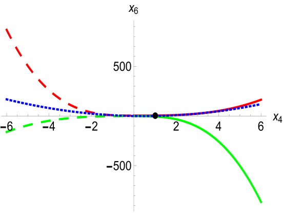
Figure 4: Region of stability in the $x_{4}-x_{6}$ plane at $|\lambda|=\frac{1}{2}$. The solid red curve represents $x_{6}-\phi_{+}+x_{4}^{3}\psi_{-}=0$ while the solid green one corresponds to $x_{6}-\phi_{-}+x_{4}^{3}\psi_{+}=0$. The dashed red curve represents the line $x_{6}-\phi_{+}+x_{4}^{3}\psi_{+}<0$ while the green dashed one denotes $x_{6}-\phi_{-}+x_{4}^{3}\psi_{-}=0$. The region between the solid red and solid green curves, and the region between the dashed red and dashed green curves define the region of stability. The blue line is the set of ${\cal N}=1$ theories while the black dot is the ${\cal N}=2$ theory. Note that all susy theories lie within the stability regime.

In Figure 4 we have shown the lines (of (3)) constraining the stability of the potential for a representative value of $|\lambda|=\frac{1}{2}$. With $x_{4}>0$, the solid red curve corresponds to $x_{6}-\phi_{+}+x_{4}^{3}\psi_{-}=0$, while the solid green one corresponds to $x_{6}-\phi_{-}+x_{4}^{3}\psi_{+}=0$. On the other hand, with $x_{4}<0$, the dashed red curve denotes $x_{6}-\phi_{+}+x_{4}^{3}\psi_{+}<0$ while the green dashed one denotes $x_{6}-\phi_{-}+x_{4}^{3}\psi_{-}=0$. The conditions (3) imply that the potential is stable only if the $x_{4}-x_{6}$ parameters lie between the solid red, solid green, dashed red and dashed green curves in Figure 4. Since the quantum effective potential at leading order in $1/N$ does not depend on the parameters $y_{4}^{\prime}$ and $y_{4}^{\prime\prime}$ in (1), our analysis does not say anything about regions of stability for those parameters.

3.1 Stability of supersymmetric theories

In this paper we are particularly interested in the $\mathcal{N}=2$ superconformal theory and deformations by its classically relevant parameters $m_{B}^{2}$, $b_{4}$ and $m_{F}$. This corresponds to setting the marginal parameters $x_{4}$ and $x_{6}$ to

$$x_{4}=1\ ,\quad x_{6}=0\ .$$ (48)

In Figure 4, the black dot at $x_{4}=1,x_{6}=0$ denotes the $\mathcal{N}=2$ SUSY point and it exists inside the region of stability.

We perform the stability analysis for general $|\lambda|$ now. The following inequalities must be satisfied for the $\mathcal{N}=2$ theory to be stable:

$$\psi_{-}<\phi_{+}\ ,\qquad\psi_{+}>\phi_{-}\ .$$ (49)

The inequalities in (49) are clearly satisfied for all values of $\lambda$ (see (2.5)) and so the ${\cal N}=2$ theory is stable.

In a similar manner, the $\mathcal{N}=1$ theory corresponds to setting

$$x_{4}=\frac{1+w}{2}\ ,\quad x_{6}=w^{2}-1\ .$$ (50)

For these values of $x_{4}$ and $x_{6}$, it is not hard to verify that the stability conditions follow from (2.5). For $|\lambda|=\tfrac{1}{2}$, the blue dotted line in Figure 4 is the $\mathcal{N}=1$ locus. As expected, it lies within the region of stability.

Thus, we see that the supersymmetric subset of theories in (1) are stable, as is expected to follow from general supersymmetry arguments.

4 Phase diagram of the $\mathcal{N}=2$ theory

As we have explained in the introduction, the $\mathcal{N}=2$ theory is defined in the UV by the choice of dimensionless parameters $x_{4}=1$, $x_{6}=0$, $y_{4}^{\prime}=4$ and $y_{4}^{\prime\prime}=0$ in the action (1). These choices define a supersymmetric fixed point of the renormalization group. This fixed point admits three relevant deformations parametrized by the massive parameters $b_{4}$, $m_{B}^{2}$ and $m_{F}$. The IR behaviour of the theory is a function of the two dimensionless ratios of these parameters. It follows that the ${\cal N}=2$ theory has a two dimensional phase diagram. In this section we will quantitatively work out this phase diagram in the large $N$ limit. Our main tool in this section is the Landau-Ginzburg effective potential is given by (42):

$$U^{(\varepsilon,\pm)}(\sigma)=\frac{N}{2\pi}\Big{[}\left(\psi_{\varepsilon}-\phi_{\pm}\right)\lambda^{2}{\sigma}^{3}+\left({b}_{4}+\tfrac{3}{4}\psi_{\varepsilon}m_{F}\right)2\lambda{\sigma}^{2}\\ +\left({m}_{B}^{2}+\tfrac{3}{4}\psi_{\varepsilon}m_{F}^{2}\right){\sigma}+\psi_{\varepsilon}\frac{m_{F}^{3}}{8\lambda}-\frac{m_{F}\left(b_{4}m_{F}-m_{B}^{2}\right)}{4\lambda}\Big{]}\ .$$ (51)

The parameter $\varepsilon=\text{sgn}(m_{F}+2\lambda\sigma)\text{sgn}(\lambda)$ measures the sign of the effective fermionic mass expanded around a vacuum with a particular value of $\sigma$; the fact that our effective potential changes discontinuously as this sign flips is a reflection of the fact that ‘phase’ as a function of $\sigma$ undergoes a continuous second order ‘phase transition’ as $m_{F}+2\lambda\sigma$ goes through zero (the level of the low energy Chern-Simons theory in the massive phase is an order parameter for this phase transition). In a similar manner, the sign in $\phi_{\pm}$ is either $+$ or $-$ depending on whether $\sigma$ is negative or positive; so, as $\sigma$ changes sign, the coefficient of the $\sigma^{3}$ term in (51) changes. This non-analyticity reflects the fact that our theory undergoes a second order Higgsing ‘phase transition’ as $\sigma$ goes from negative to positive values (the rank of the low energy Chern-Simons theory in the massive phase is an order parameter for this phase transition).

The quantities $\phi_{\pm}$ and $\psi_{\pm}$ are defined in (44) and (43) respectively and are reproduced below:

$$\phi_{+}=\frac{4}{3}\left(\frac{1}{\lambda^{2}}-1\right)\ ,\quad \phi_{-}=\frac{4}{3}\left(\frac{1}{(2-|\lambda|)^{2}}-1\right)\ ,$$

$$\psi_{+}=\frac{4}{3}\left(\frac{1}{(1-|\lambda|)^{2}}-1\right)\ ,\quad \psi_{-}=\frac{4}{3}\left(\frac{1}{(1+|\lambda|)^{2}}-1\right)\ ,$$ (52)

along with their ordering:

$$1\geq|\lambda|\geq\frac{1}{2}: \quad\psi_{+}\geq\phi_{+}\geq 0\geq\phi_{-}\geq\psi_{-}\ ,$$

$$0\leq|\lambda|<\frac{1}{2}: \quad\phi_{+}>\psi_{+}\geq 0\geq\psi_{-}>\phi_{-}\ .$$ (53)

Note that this ordering of $\phi_{\pm}$ and $\psi_{\pm}$ ensures that the coefficient of $\sigma^{3}$ in (51) is manifestly positive/negative at asymptotically large positive/negative values of $\sigma$; This ensures that the potential (51) is bounded from below for all values of $|\lambda|$.

From the expression for the potential above in (51) it is apparent that an odd power of $m_{F}$ always appears with a $\lambda$ and similarly, every occurrence of an odd power of $b_{4}$ is accompanied by a $\lambda$. Thus, our theory depends only on the combinations $m_{F}\text{sgn}(\lambda)$ and $\lambda b_{4}$.

Our Landau-Ginzburg potential depends on three dimensionful parameters in addition to the dimensionless coupling $\lambda$. Of course, all information about the phase diagram is invariant under changes of units under which dimensionful parameters transform as

$$m_{F}\rightarrow\alpha m_{F}\ ,\quad b_{4}\rightarrow\alpha b_{4}\ ,\quad m_{B}^{2}\rightarrow\alpha^{2}m_{B}^{2}\ ,$$ (54)

where $\alpha$ is any positive number. In other words the three dimensional parameter space parametrized by $m_{F}$, $b_{4}$ and $m_{B}^{2}$ can be foliated by the ellipsoid-like surfaces given by

$$(m_{B}^{2})^{2}+(m_{F}^{2}+(\lambda b_{4})^{2})^{2}=\text{constant}\ .$$ (55)

for various different positive values of the constant. The ‘scale symmetry’ (54) ensures that we lose no information by studying our theory at any given positive value of the constant in (55); in other words the phase diagram of our theory lives on the surface (55) at any convenient value of the constant. Also note that the $\mathcal{N}=2$ superconformal theory itself lives at the origin of the three dimensional parameter space $(m_{B}^{2},\lambda b_{4},m_{F}\text{sgn}(\lambda))=(0,0,0)$.

We will use the following terminology in the rest of this paper. We call the part of the ‘ellipsoid’ (55) that lies in the region $m_{F}\text{sgn}(\lambda)>0$ as the northern hemisphere of the ellipsoid. In a similar manner, we will call the part of the ellipsoid that lies in the region $m_{F}\text{sgn}(\lambda)<0$ the southern hemisphere. Finally, the intersection of the plane $m_{F}=0$ and the ellipsoid is a curve that we call the equator of the ellipsoid.

All information about the phase diagram of the theory in its northern hemisphere can be obtained (using the scaling (54)) from the study of the theory at any fixed positive value of $m_{F}\text{sgn}(\lambda)$. Similarly all information about the theory on its southern hemisphere can be obtained by studying the theory at any fixed negative value of $m_{F}\text{sgn}(\lambda)$. Finally, the information about the theory along the equator can clearly be obtained by studying the theory at $m_{F}=0$. In the rest of this section we will separately study the theory on the ‘horizontal’ sections $m_{F}=0$, at $m_{F}=|\mu|{\rm sgn}(\lambda)$ and at $m_{F}=-|\mu|{\rm sgn}(\lambda)$ and then finally put together the phase diagram by patching these results together (in order to achieve this patching in a smooth way we also separately study a neighbourhood of the equator). We begin our analysis with the simplest case, namely the study of the equator.

4.1 The equator: $m_{F}=0$

In this case the sign $\varepsilon=\text{sgn}(m_{F}+2\lambda\sigma)\text{sgn}(\lambda)$ that decides the fermionic phase simplifies:

$$\varepsilon=\text{sgn}(\lambda\sigma)\text{sgn}(\lambda)=\text{sgn}(\sigma)\ .$$ (56)

This implies that the fermionic phase is tied to the bosonic phase: when the boson is in the Higgsed / unHiggsed ($\mp$) phase, the fermion is in the $\pm$ phase. In other words, when the boson undergoes a phase transition, the fermion undergoes a phase transition as well. Thus, the effective potential (51) at $m_{F}=0$ accesses only two phases viz. $(-,+)$ and $(+,-)$. The explicit expression for the Landau-Ginzburg potential (51) collapses to a form very similar to that of the regular boson theory (Equation (124) in Appendix A):

$$U(\sigma)=\frac{N}{2\pi}\left\{\begin{array}[]{cl}(\psi_{-}-\phi_{+})\lambda^{2}{\sigma}^{3}+2\lambda b_{4}{\sigma}^{2}+m_{B}^{2}{\sigma}&\quad\text{for $\sigma<0$ i.e.~{}the $(-,+)$ phase}\ ,\\ (\psi_{+}-\phi_{-})\lambda^{2}{\sigma}^{3}+2\lambda{b}_{4}{\sigma}^{2}+{m}_{B}^{2}{\sigma}&\quad\text{for $\sigma>0$ i.e.~{}the $(+,-)$ phase}\ .\end{array}\right.$$ (57)

Figure 5: The $m_{F}=0$ section of the paraboloids in (4.1) is given in Figure (a). The inset plots are the profiles of the LG potential (57) with the horizontal axis being the $\sigma$ axis and the vertical axis being the value of the potential. Across the blue line the minimum of the potential passes through $\sigma=0$. Along the red line a local maximum of the LG potential passes through $\sigma=0$. The dashed lines correspond to either the appearance or disappearance of new extrema in the potential. The phase structure is given in Figure (b) with the blue line denoting a second order Higgsing phase transition and the green line denoting a numerically-determined first order phase transition. The ellipse (eq. (59)) is the intersection of the two dimensional plane with the ellipsoid (55). The first order line lies to the right of the diagram - as depicted in the figure above - when $|\lambda|<\frac{1}{2}$ but moves to the left of the figure for $|\lambda|>\frac{1}{2}$. It runs exactly down the negative $\lambda b_{4}$ axis at $|\lambda|=\frac{1}{2}$.

We see that the above potential is stable (following the inequalities in (4)) and hence the analysis can be borrowed from the regular boson analysis for the case $\phi_{-}<x_{6}^{B}<\phi_{+}$ in Dey:2018ykx or in Section A.1.4 of Appendix A in this paper. Note that the value of $x_{6}^{B}$ under which (57) reduces to the regular boson theory is $\psi_{-}$ for $\sigma<0$ and $\psi_{+}$ for $\sigma>0$, as opposed to a single value of $x_{6}^{B}$ for both branches in the actual regular boson theory. For this reason the analysis in the present case has minor quantitative differences compared to that of the regular boson. We present the analytic features of the potential in Figure 5(a). The main features are the following half-parabolas:

$$L_{0}: \quad m_{B}^{2}=0\ ,\quad\lambda b_{4}>0\ ,$$

$$M_{0}: \quad m_{B}^{2}=0\ ,\quad\lambda b_{4}<0\ ,$$

$$D_{h0}: \quad 16(\lambda b_{4})^{2}-12\lambda^{2}(\psi_{+}-\phi_{-})m_{B}^{2}=0\ ,\quad\lambda b_{4}<0\ ,$$

$$D^{\prime}_{u0}: \quad 16(\lambda b_{4})^{2}-12\lambda^{2}(\psi_{-}-\phi_{+})m_{B}^{2}=0\ ,\quad\lambda b_{4}<0\ .$$ (58)

The half-parabola $L_{0}$ is significant because a minimum of the potential goes from the range $\sigma>0$ to the range $\sigma<0$ and hence goes from the $(+,-)$ phase to the $(-,+)$ phase (and vice versa). Thus, $L_{0}$ corresponds to a second order phase transition between the above two phases. Similarly, the half-line $M_{0}$ corresponds to a maximum of the potential crossing $\sigma=0$. The half-parabolas $D^{\prime}_{u0}$ and $D_{h0}$ correspond to the (dis)appearance of new extrema of the potential as one crosses them. For instance, above the $D^{\prime}_{u0}$ half-parabola, the potential has a single minimum, while below it there are two minima and one maximum.

The phase structure is obtained by determining the global minimum in different regions of parameter space $(m_{B}^{2},\lambda b_{4})$. There are two competing minima in different phases in the region below $D^{\prime}_{u0}$ and $D_{h0}$ in Figure 5. The dominant minimum has to be numerically determined in this region. The line across which the minimum in one phase becomes dominant over the other defines a first-order phase boundary between the two phases. We present the second order and the first order phase transition lines in Figure 5(b).

Above, we determined the phase structure for $m_{F}=0$ as a function of two dimensionful parameters $m_{B}^{2}$ and $\lambda b_{4}$. As discussed at the beginning of this section around equation (55), the actual phase diagram is two dimensional and lives on the ellipsoid (55). The intersection of the $m_{F}=0$ slice with this ellipsoid is given by the equatorial ‘ellipse’

$$(\lambda b_{4})^{4}+(m_{B}^{2})^{2}=\text{constant}\ ,$$ (59)

as depicted in Figure 5(b). The blue line and the green line in Figure 5 intersect this ellipse at one point each, corresponding to a second order and a first order phase transition respectively on the equator of the phase diagram ellipsoid (55).

4.1.1 The CB-RF conformal theory

We commented earlier around equation (56) in this subsection that whenever a boson undergoes a phase transition, the fermion undergoes a phase transition as well. Recall that the minimum of the potential goes to zero on the half-line

$$\lambda b_{4}>0\ ,\quad m_{B}^{2}=0\ ,$$ (60)

and hence the gaps $c_{B}$, $c_{F}$ in (2.5) go to zero as well. Thus, this corresponds to a phase transition for both the boson and the fermion. The above half-line intersects the ellipse (59) at one point. The conformal dynamics at this point is then presumably governed by a theory of critical bosons and regular fermions coupled to a $SU(N)_{k}$ Chern-Simons theory.

We give more evidence for this statement in the sections below when we study the $\mathcal{N}=2$ theory at non-zero $m_{F}$ which, at small values of $m_{F}$, should correspond to particular massive deformations of this CB-RF conformal theory. We also obtain precisely this CB-RF point as a scaling limit of the general theory (1) in Section (D.3) of Appendix D.

4.2 The northern hemisphere: $\textnormal{sgn}(m_{F})=\textnormal{sgn}(\lambda)$

We next consider the case $\text{sgn}(m_{F})\text{sgn}(\lambda)=+1$. The regions of validity for the various branches of the potential are in Figure 6.

Figure 6: Regions of validity for different branches of the potential for $\text{sgn}(m_{F})\text{sgn}(\lambda)=+1$.

The appropriate expressions for the potential are

$$U(\sigma)=\frac{N}{2\pi}\left\{\begin{array}[]{lr}\begin{array}[]{r}\left({m}_{B}^{2}+\frac{3}{4}\psi_{-}m_{F}^{2}\right)\sigma+\left({b}_{4}+\tfrac{3}{4}\psi_{-}m_{F}\right)2\lambda\sigma^{2}\\ +(\psi_{-}-\phi_{+})\lambda^{2}\sigma^{3}+\frac{\psi_{-}-\psi_{+}}{8\lambda}m_{F}^{3}\end{array}\ ,&\sigma<-\frac{m_{F}}{2\lambda}\ ,\\ \begin{array}[]{r}\left({m}_{B}^{2}+\frac{3}{4}\psi_{+}m_{F}^{2}\right)\sigma+\left({b}_{4}+\frac{3}{4}\psi_{+}m_{F}\right)2\lambda\sigma^{2}\\ +(\psi_{+}-\phi_{+})\lambda^{2}\sigma^{3}\end{array}\ ,&-\frac{m_{F}}{2\lambda}<\sigma<0\ ,\\ \begin{array}[]{r}\left({m}_{B}^{2}+\frac{3}{4}\psi_{+}m_{F}^{2}\right)\sigma+\left({b}_{4}+\frac{3}{4}\psi_{+}m_{F}\right)2\lambda\sigma^{2}\\ +(\psi_{+}-\phi_{-})\lambda^{2}\sigma^{3}\end{array}\ ,&\sigma>0\ .\end{array}\right.$$ (61)

We have subtracted an overall constant $-\frac{m_{F}(b_{4}m_{F}-m_{B}^{2})}{4\lambda}+\frac{\psi_{+}}{8\lambda}m_{F}^{3}$ from all the expressions above.

It helps to consider the interfaces $\sigma=0$ and $\sigma=-\frac{m_{F}}{2\lambda}$ separately. We write the potential in a coordinate that is zero at the corresponding interface:

$${U}(\sigma)=\frac{N}{2\pi}\left\{\begin{array}[]{lr}\begin{array}[]{r}\left({m}_{B}^{2}+\frac{3}{4}\psi_{+}m_{F}^{2}\right)\sigma+\left({b}_{4}+\frac{3}{4}\psi_{+}m_{F}\right)2\lambda\sigma^{2}\\ +(\psi_{+}-\phi_{+})\lambda^{2}\sigma^{3}\end{array}\ ,&-\frac{m_{F}}{2\lambda}<\sigma<0\ ,\\ \begin{array}[]{r}\left({m}_{B}^{2}+\frac{3}{4}\psi_{+}m_{F}^{2}\right)\sigma+\left({b}_{4}+\frac{3}{4}\psi_{+}m_{F}\right)2\lambda\sigma^{2}\\ +(\psi_{+}-\phi_{-})\lambda^{2}\sigma^{3}\end{array}\ ,&\sigma>0\ .\end{array}\right.$$ (62)

$${U}^{\prime}(\sigma^{\prime})=\frac{N}{2\pi}\left\{\begin{array}[]{lr}\begin{array}[]{r}\left({m}_{B}^{2}-2{b}_{4}m_{F}-\frac{3}{4}\phi_{+}m_{F}^{2}\right)\sigma^{\prime}+\left({b}_{4}+\tfrac{3}{4}\phi_{+}m_{F}\right)2\lambda\sigma^{\prime}{}^{2}\\ +(\psi_{-}-\phi_{+})\lambda^{2}\sigma^{\prime}{}^{3}\end{array}\ ,&\sigma^{\prime}<0\ ,\\ \begin{array}[]{r}\left({m}_{B}^{2}-2{b}_{4}m_{F}-\frac{3}{4}\phi_{+}m_{F}^{2}\right)\sigma^{\prime}+\left({b}_{4}+\tfrac{3}{4}\phi_{+}m_{F}\right)2\lambda\sigma^{\prime}{}^{2}\\ +(\psi_{+}-\phi_{+})\lambda^{2}\sigma^{\prime}{}^{3}\end{array}\ ,&0<\sigma^{\prime}<\frac{m_{F}}{2\lambda}\ .\end{array}\right.$$ (63)

where ${\sigma^{\prime}}={\sigma}+\frac{m_{F}}{2\lambda}$. There is an additional common constant

$$\tfrac{1}{8\lambda}(4{b}_{4}m_{F}^{2}-4{m}_{B}^{2}m_{F}+m_{F}^{3}(\phi_{+}-\psi_{+}))$$

in both the lines above in (63). This is the relative shift compared to the potential in terms of $\sigma$ above in (62). To re-emphasize, in the region where $U(\sigma)$ and $U^{\prime}(\sigma^{\prime})$ are both valid (i.e. for $-\frac{m_{F}}{2\lambda}<\sigma<0$) the two potentials are related via

$$U(\sigma)=U^{\prime}(\sigma+\tfrac{m_{F}}{2\lambda})+\tfrac{1}{8\lambda}(4{b}_{4}m_{F}^{2}-4{m}_{B}^{2}m_{F}+m_{F}^{3}(\phi_{+}-\psi_{+}))$$ (64)

Our strategy for the rest of this subsection is the following. We will work out the phase diagram separately for the potential $U(\sigma)$ (pretending that it was valid at all values of $\sigma$) and for $U^{\prime}(\sigma^{\prime})$ (again pretending it was valid for all values of $\sigma^{\prime}$) and then finally patch these two results together in order to get the actual phase diagram of the system - this time taking care to use the results for $U$ and $U^{\prime}$ only within their domains of validity i.e. $-\tfrac{m_{F}}{2\lambda}<\sigma$ and $\sigma^{\prime}<\tfrac{m_{F}}{2\lambda}$ respectively.

The analysis for the two sets of potentials in (62) and (63) proceeds in the same way as that of the regular boson theory (see Appendix A of this paper). The potential $U(\sigma)$ in (62) is stable when $\phi_{-}<\psi_{+}<\phi_{+}$. From the ordering given in (4), it is clear that this is case when $|\lambda|<\frac{1}{2}$.

Thus, in this case, the analysis of the regular boson for $\phi_{-}<x_{6}^{B}<\phi_{+}$ applies (See Section A.1.4 of Appendix A). There are four semi-infinite surfaces (half-paraboloids) that are important in describing the profile of the potential around $\sigma=0$. These are given by the following conditions:

$$L:\ m_{B}^{2}+\tfrac{3}{4}\psi_{+}m_{F}^{2}=0\ ,\quad\lambda(b_{4}+\tfrac{3}{4}\psi_{+}m_{F})>0\ ,$$

$$M:\ m_{B}^{2}+\tfrac{3}{4}\psi_{+}m_{F}^{2}=0\ ,\quad\lambda(b_{4}+\tfrac{3}{4}\psi_{+}m_{F})<0\ ,$$

$$D_{u}:\ 16(\lambda b_{4}+\tfrac{3}{4}\psi_{+}\lambda m_{F})^{2}-12\lambda^{2}(\psi_{+}-\phi_{+})(m_{B}^{2}+\tfrac{3}{4}\psi_{+}m_{F}^{2})=0\ ,\quad\lambda(b_{4}+\tfrac{3}{4}\psi_{+}m_{F})<0\ ,$$

$$D_{h}:\ 16(\lambda b_{4}+\tfrac{3}{4}\psi_{+}\lambda m_{F})^{2}-12\lambda^{2}(\psi_{+}-\phi_{-})(m_{B}^{2}+\tfrac{3}{4}\psi_{+}m_{F}^{2})=0\ ,\quad\lambda(b_{4}+\tfrac{3}{4}\psi_{+}m_{F})<0\ .$$ (65)

Our notation for these curves parallels that used in the regular boson analysis in Section A.1.4 in Appendix A. The significance of these surfaces is the following. Across the surface $L$ the minimum of the effective potential (62) goes from the range $\sigma<0$ to the range $\sigma>0$ or vice-versa. This signals a second order phase transition. Similarly, as one crosses the surface $M$ a local maximum of the effective potential (62) crosses $\sigma=0$. The surfaces $D_{u}$ and $D_{h}$ are such that when one crosses them the effective potential (62) develops or loses a maximum-minimum pair.

In this same range of $|\lambda|<\tfrac{1}{2}$, the potential $U^{\prime}(\sigma^{\prime})$ in (63) is unbounded from below at large positive $\sigma^{\prime}$ for $\sigma^{\prime}>0$. Thus, the $x_{6}^{B}<\phi_{-}$ analysis of the regular boson theory is applicable here. Again, there are four half-paraboloids that are important for the profile of the potential around $\sigma^{\prime}=0$ i.e. $\sigma=-\frac{m_{F}}{2\lambda}$:

$$L^{\prime}:\ m_{B}^{2}-2\lambda b_{4}\frac{m_{F}}{\lambda}-\tfrac{3}{4}\phi_{+}m_{F}^{2}=0\ ,\quad\lambda(b_{4}+\tfrac{3}{4}\phi_{+}m_{F})>0\ ,$$

$$M^{\prime}:\ m_{B}^{2}-2\lambda b_{4}\frac{m_{F}}{\lambda}-\tfrac{3}{4}\phi_{+}m_{F}^{2}=0\ ,\quad\lambda(b_{4}+\tfrac{3}{4}\phi_{+}m_{F})<0\ ,$$

$$D^{\prime}_{u}:\ \left\{\begin{array}[]{l}16(\lambda b_{4}+\tfrac{3}{4}\phi_{+}\lambda m_{F})^{2}-12\lambda^{2}(\psi_{-}-\phi_{+})(m_{B}^{2}-2b_{4}m_{F}-\tfrac{3}{4}\phi_{+}m_{F}^{2})=0\ ,\\ \lambda(b_{4}+\tfrac{3}{4}\phi_{+}m_{F})<0\ ,\end{array}\right.$$ (68)

$$D^{\prime}_{h}:\ \left\{\begin{array}[]{l}16(\lambda b_{4}+\tfrac{3}{4}\phi_{+}\lambda m_{F})^{2}-12\lambda^{2}(\psi_{+}-\phi_{+})(m_{B}^{2}-2b_{4}m_{F}-\tfrac{3}{4}\phi_{+}m_{F}^{2})=0\\ \lambda(b_{4}+\tfrac{3}{4}\phi_{+}m_{F})>0\ .\end{array}\right.$$ (71)

As above, the surfaces $L^{\prime}$ and $M^{\prime}$ denote the lines across which the minimum or a local maximum, respectively, of $U^{\prime}(\sigma^{\prime})$ crosses $\sigma^{\prime}=0$. The surfaces $D_{u}^{\prime}$ and $D^{\prime}_{h}$ denote locations of nucleation of new extrema of $U^{\prime}(\sigma^{\prime})$.

Recall that $D_{u}$ and $D^{\prime}_{h}$ both correspond to surfaces across which the potentials $U(\sigma)$ and $U^{\prime}(\sigma^{\prime})$ develop new extrema. It turns out that the special value of $\sigma$ at which these new extrema are nucleated lies in the region $-\frac{m_{F}}{2\lambda}<\sigma<0$ where the potentials $U(\sigma)$ and $U^{\prime}(\sigma^{\prime})$ are both valid (see Figure 7(a)). For this reason $D_{u}$ and $D^{\prime}_{h}$ define the exact same paraboloid.

As we have explained in the introduction to this section, all information of the phase diagram in the upper hemisphere (i.e. when $m_{F}\lambda>0$) can be extracted (by scaling) from the free energy at a fixed positive value of $m_{F}\lambda$, let us say on the ‘horizontal section’

$$m_{F}=|\mu|\,\text{sgn}(\lambda)\ .$$ (72)

We make this choice in what follows. All our final results can in fact be recast as functions of the two variables

$$\frac{\lambda b_{4}}{|\mu|}\equiv\frac{\lambda b_{4}}{m_{F}\text{sgn}(\lambda)}\ ,\quad\frac{m_{B}^{2}}{\mu^{2}}\equiv\frac{m_{B}^{2}}{m_{F}^{2}}\ ,$$ (73)

which can be thought of as a set of ‘coordinates’ on the upper hemisphere of the phase diagram. We next give a detailed description of the analytic features and the phase structure of the potential $U(\sigma)$ for $\text{sgn}(m_{F})=\text{sgn}(\lambda)$ in Figures 7 and 8.

Figure 7: The $m_{F}=|\mu|\,\text{sgn}(\lambda)$ section of the paraboloids in (4.2) and (4.2) for $|\lambda|<\tfrac{1}{2}$. Each of the inset pair-of-plots in Figure (a) correspond to the profiles of the potential $U^{\prime}(\sigma^{\prime})$ (the plot on the left) and $U(\sigma)$ (the plot on the right). The vertical lines in each of these plots correspond to the points $\sigma^{\prime}=0$ and $\sigma=0$ respectively. The inset plots in Figure (b) are the profiles of the potential (61) and the two vertical lines in these plots correspond to $\sigma=-m_{F}/2\lambda$ and $\sigma=0$ respectively. The blue lines correspond to a minimum of the local potential crossing the vertical axis while the red lines correspond to a maximum crossing the vertical axis. The dashed and dotted lines correspond to either the appearance or disappearance of new extrema in the potential.

Figure 8: Deducing the phase structure for the $m_{F}=|\mu|\,\text{sgn}(\lambda)$ section for $|\lambda|<\tfrac{1}{2}$. The inset plots are the profiles of the potential (61). The two vertical lines in each plot correspond to $\sigma=-m_{F}/2\lambda$ and $\sigma=0$ and demarcate the regions of validity of the $(-,+)$, $(+,+)$ and $(+,-)$ branches of the potential (61) (cf. Figure 6). The green line in Figure (b) corresponds to a numerically-determined first order transition line. It meets the second order transition line $L^{\prime}$ emanating from the point ${\rm CF}+$ at the point ${\rm O}+$.

We first give a brief explanation of the features of Figure 7. The intersections of the paraboloids in (4.2) , (4.2) with the $m_{F}=|\mu|\text{sgn}(\lambda)$ slice yield parabolas and we use the same notation to describe these as their parent paraboloids.

1. We depict the profiles of the potentials $U(\sigma)$ (62) and $U^{\prime}(\sigma^{\prime})$ (63) in the $(m_{B}^{2},\lambda b_{4})$ space for each of the regions demarcated by the curves $L$, $M$, $L^{\prime}$, $M^{\prime}$, $D_{u}$, $D_{h}$, $D^{\prime}_{u}$, $D^{\prime}_{h}$ in Figure 7(a). In each region we display a pair of small plots: the plot on the left is the potential $U^{\prime}(\sigma^{\prime})$ in the neighbourhood of $\sigma^{\prime}=0$ ($\sigma=-\tfrac{m_{F}}{2\lambda}$) and the plot on the right is the potential $U(\sigma)$ in the neighbourhood of $\sigma=0$. All plots are based on the regular boson analysis in Dey:2018ykx (or in Appendix A of this paper). Note that as one crosses the various lines ($L$, $M$, etc.), the plots of the potential (62) and (63) qualitatively change. The points ${\rm RB}+$ and ${\rm CF}+$ at which the second order lines $L$ and $L^{\prime}$ end are precisely the location of the RB and CF scaling limits given in (217) and (198) respectively.

2. Since the pair of graphs in Figure 7(a) belong to the same continuous potential given in (61), we have to patch the two graphs in the region between $\sigma=-\frac{m_{F}}{2\lambda}$ and $\sigma=0$ such that the continuity is maintained. The final profile of the potential (61) in each region is given in Figure 7(b). As we can see from Figure 7(b), the curves $D_{h}^{\prime}$ (above RB$+$) and $D_{u}$ (below CF$+$) are superfluous since the nature of the potential remains the same when one crosses them. Figure 7(b) contains complete analytic information about the Landau-Ginzburg potential for $\text{sgn}(m_{F})\text{sgn}(\lambda)=+1$.

We are also interested in the phase structure of the potential (61). In other words, we focus on the minima of the potential in various regions of the parameter space $(m_{B}^{2},\lambda b_{4})$ at fixed $m_{F}=|\mu|\text{sgn}(\lambda)$. This is summarised in Figure 8.

1. One needs to study the profiles of the potential in Figure 7(b) in more detail, possibly making use of numerical methods. For instance, in the region below the dotted and dashed curves in Figure 8(a), there are two competing minima. There is a first order phase boundary that separates the regions where one minimum dominates over the other. This boundary has to be determined numerically by computing the two local minimum values of the potential and the boundary is located at the parameter values where these two minimum values are equal. We give a schematic depiction of this first order line as the green line in Figure 8(b). In Appendix C, we give a detailed description of the numerics along with the required plots.

2. The dynamics on the second order transition line $L$ in Figure 8 is governed by the conformal critical boson theory ${\rm CB}+$ and terminates at the point ${\rm RB}+$ which is governed by a theory of conformal regular bosons i.e. free bosons (the $+$ indicates that fermions are gapped in the neighbourhood of the line and are in the $+$ phase). This second order phase transition separates the $(+,+)$ and the $(+,-)$ phases. The phase transition continues beyond ${\rm RB}+$ but now switches to being a first order transition between the phases $(+,+)$ and $(+,-)$ till the point ${\rm O}+$. Beyond the point ${\rm O}+$, the phase transition is still first order but now separates the $(-,+)$ and the $(+,-)$ phases.

   Similarly, the line $L^{\prime}$ in Figure 8 corresponds to the regular fermion theory ${\rm RF}+$ and it ends at ${\rm O}+$ on the first order line that emanates out of ${\rm RB}+$ (the $+$ indicates that the gapped boson is in the $+$ phase in the neighbourhood of this line). This second order phase transition separates the $(+,+)$ and the $(-,+)$ phases. Till the point ${\rm O}+$ the dominant minimum undergoes the second order phase transition. At this point ${\rm O}+$, it switches to being a subdominant minimum and hence becomes unimportant as far as the phase structure is concerned.

3. Note that if one sets $m_{F}=0$ in the surfaces $L$ and $L^{\prime}$ in (4.2) and (4.2), one gets back the straight line $L_{0}$ in the case $m_{F}=0$ in (4.1) and in Figure 5. Thus, the ${\rm CB}+$ and ${\rm RF}+$ paraboloids intersect with each other along the line $L_{0}$ on the $m_{F}=0$ section. Recall that this line $L_{0}$ describes the CB-RF conformal theory. In Section 4.4, we map the lines $L$ and $L^{\prime}$ onto the ellipsoid (55) and we shall see that they converge to the CB-RF point on equator of the ellipsoid that was described in Section 4.1.1.

4.3 The southern hemisphere: $\textnormal{sgn}(m_{F})=-\textnormal{sgn}(\lambda)$

This choice of $\text{sgn}(m_{F})$ accesses the $(-,+)$, $(-,-)$ and the $(+,-)$ branches of the Landau-Ginzburg potential. The regions of validity for the various branches on the $\sigma$ axis are displayed in Figure 9.

Figure 9: Regions of validity for different branches of the potential for $\text{sgn}(m_{F})\text{sgn}(\lambda)=-1$.

The corresponding expressions for the potential in the various branches are

$${\tilde{U}}(\sigma)=\frac{N}{2\pi}\left\{\begin{array}[]{lr}\begin{array}[]{r}\left({m}_{B}^{2}+\frac{3}{4}\psi_{-}m_{F}^{2}\right)\sigma+\left({b}_{4}+\tfrac{3}{4}\psi_{-}m_{F}\right)2\lambda\sigma^{2}\\ +(\psi_{-}-\phi_{+})\lambda^{2}\sigma^{3}\end{array},&\sigma<0\ ,\\ \begin{array}[]{r}\left({m}_{B}^{2}+\frac{3}{4}\psi_{-}m_{F}^{2}\right)\sigma+\left({b}_{4}+\frac{3}{4}\psi_{-}m_{F}\right)2\lambda\sigma^{2}\\ +(\psi_{-}-\phi_{-})\lambda^{2}\sigma^{3}\end{array}\ ,&0<\sigma<-\frac{m_{F}}{2\lambda}\ ,\\ \begin{array}[]{r}\left({m}_{B}^{2}+\frac{3}{4}\psi_{+}m_{F}^{2}\right)\sigma+\left({b}_{4}+\frac{3}{4}\psi_{+}m_{F}\right)2\lambda\sigma^{2}\\ +(\psi_{+}-\phi_{-})\lambda^{2}\sigma^{3}+\frac{\psi_{+}-\psi_{-}}{8\lambda}m_{F}^{3}\end{array}\ ,&\sigma>-\frac{m_{F}}{2\lambda}\ .\end{array}\right.$$ (74)

We have subtracted an overall constant $-\frac{m_{F}(b_{4}m_{F}-m_{B}^{2})}{4\lambda}+\frac{\psi_{-}}{8\lambda}m_{F}^{3}$ from all the expressions above for brevity.

Again, it helps to consider the interfaces $\sigma=0$ and $\sigma=-\frac{m_{F}}{2\lambda}$ separately and write the potential in an coordinate that is zero at the corresponding interface:

$${\tilde{U}}(\sigma)=\frac{N}{2\pi}\left\{\begin{array}[]{lr}\begin{array}[]{r}\left({m}_{B}^{2}+\frac{3}{4}\psi_{-}m_{F}^{2}\right)\sigma+\left({b}_{4}+\frac{3}{4}\psi_{-}m_{F}\right)2\lambda\sigma^{2}\\ +(\psi_{-}-\phi_{+})\lambda^{2}\sigma^{3}\end{array}\ ,&\sigma<0\ ,\\ \begin{array}[]{r}\left({m}_{B}^{2}+\frac{3}{4}\psi_{-}m_{F}^{2}\right)\sigma+\left({b}_{4}+\frac{3}{4}\psi_{-}m_{F}\right)2\lambda\sigma^{2}\\ +(\psi_{-}-\phi_{-})\lambda^{2}\sigma^{3}\end{array}\ ,&0<\sigma<-\frac{m_{F}}{2\lambda}\ .\end{array}\right.$$ (75)

$${\tilde{U}}^{\prime}(\sigma^{\prime})=\frac{N}{2\pi}\left\{\begin{array}[]{lr}\begin{array}[]{r}\left({m}_{B}^{2}-2{b}_{4}m_{F}-\frac{3}{4}\phi_{-}m_{F}^{2}\right)\sigma^{\prime}+\left({b}_{4}+\tfrac{3}{4}\phi_{-}m_{F}\right)2\lambda\sigma^{\prime}{}^{2}\\ +(\psi_{-}-\phi_{-})\lambda^{2}\sigma^{\prime}{}^{3}\end{array}\ ,&\frac{m_{F}}{2\lambda}<\sigma^{\prime}<0\ ,\\ \begin{array}[]{r}\left({m}_{B}^{2}-2{b}_{4}m_{F}-\frac{3}{4}\phi_{-}m_{F}^{2}\right)\sigma^{\prime}+\left({b}_{4}+\tfrac{3}{4}\phi_{-}m_{F}\right)2\lambda\sigma^{\prime}{}^{2}\\ +(\psi_{+}-\phi_{-})\lambda^{2}\sigma^{\prime}{}^{3}\end{array}\ ,&\sigma^{\prime}>0\ .\end{array}\right.$$ (76)

where ${\sigma^{\prime}}={\sigma}+\frac{m_{F}}{2\lambda}$. There is an additional common constant

$$\tfrac{1}{8\lambda}(4{b}_{4}m_{F}^{2}-4{m}_{B}^{2}m_{F}+m_{F}^{3}(\phi_{-}-\psi_{-}))$$

in both the expressions above in (76). This is the relative shift compared to the potential in terms of $\sigma$ above in (75).

Again, we can apply the regular boson analysis as in the previous subsection. We stick to the range $|\lambda|<\tfrac{1}{2}$ as in the previous cases. In this range of $|\lambda|$, the potential ${\tilde{U}}(\sigma)$ in (75) is stable (i.e. bounded below for both $\sigma>0$ and $\sigma<0$). However, the potential ${\tilde{U}}^{\prime}(\sigma^{\prime})$ in (76) is unbounded below for $\sigma^{\prime}<0$ and bounded below for $\sigma^{\prime}>0$, making it unstable. First, we consider the potential ${\tilde{U}}(\sigma)$ in (75). As earlier, there are four semi-infinite surfaces that are important for our analysis:

$${\tilde{L}}:\ m_{B}^{2}+\tfrac{3}{4}\psi_{-}m_{F}^{2}=0\ ,\quad\lambda(b_{4}+\tfrac{3}{4}\psi_{-}m_{F})>0\ ,$$

$${\tilde{M}}:\ m_{B}^{2}+\tfrac{3}{4}\psi_{-}m_{F}^{2}=0\ ,\quad\lambda(b_{4}+\tfrac{3}{4}\psi_{-}m_{F})<0\ ,$$

$${\tilde{D}}_{u}:\ 16(\lambda b_{4}+\tfrac{3}{4}\psi_{-}\lambda m_{F})^{2}-12\lambda^{2}(\psi_{-}-\phi_{+})(m_{B}^{2}+\tfrac{3}{4}\psi_{-}m_{F}^{2})=0\ ,\quad\lambda(b_{4}+\tfrac{3}{4}\psi_{-}m_{F})<0\ ,$$

$${\tilde{D}}_{h}:\ 16(\lambda b_{4}+\tfrac{3}{4}\psi_{-}\lambda m_{F})^{2}-12\lambda^{2}(\psi_{-}-\phi_{-})(m_{B}^{2}+\tfrac{3}{4}\psi_{-}m_{F}^{2})=0\ ,\quad\lambda(b_{4}+\tfrac{3}{4}\psi_{-}m_{F})<0\ .$$ (77)

Next, we focus on the potential ${\tilde{U}}^{\prime}(\sigma^{\prime})$ in (76) which is unbounded from below for $\sigma^{\prime}<0$. Thus, the case $x_{6}^{B}>\phi_{+}$ of the regular boson theory applies (see Section A.1.4 of Appendix A). Again, there are four semi-infinite surfaces that are important for the profile of the potential around $\sigma^{\prime}=0$ i.e. $\sigma=-\frac{m_{F}}{2\lambda}$:

$${\tilde{L}}^{\prime}:\ m_{B}^{2}-2\lambda b_{4}\frac{m_{F}}{\lambda}-\tfrac{3}{4}\phi_{-}m_{F}^{2}=0\ ,\quad\lambda(b_{4}+\tfrac{3}{4}\phi_{-}m_{F})>0\ ,$$

$${\tilde{M}}^{\prime}:\ m_{B}^{2}-2\lambda b_{4}\frac{m_{F}}{\lambda}-\tfrac{3}{4}\phi_{-}m_{F}^{2}=0\ ,\quad\lambda(b_{4}+\tfrac{3}{4}\phi_{-}m_{F})<0\ ,$$

$${\tilde{D}}^{\prime}_{u}:\ \left\{\begin{array}[]{l}16(\lambda b_{4}+\tfrac{3}{4}\phi_{-}\lambda m_{F})^{2}-12\lambda^{2}(\psi_{-}-\phi_{-})(m_{B}^{2}-2b_{4}m_{F}-\tfrac{3}{4}\phi_{-}m_{F}^{2})=0\ ,\\ \lambda(b_{4}+\tfrac{3}{4}\phi_{-}m_{F})<0\ ,\end{array}\right.$$ (80)

$${\tilde{D}}^{\prime}_{h}:\ \left\{\begin{array}[]{l}16(\lambda b_{4}+\tfrac{3}{4}\phi_{-}\lambda m_{F})^{2}-12\lambda^{2}(\psi_{+}-\phi_{-})(m_{B}^{2}-2b_{4}m_{F}-\tfrac{3}{4}\phi_{-}m_{F}^{2})=0\ ,\\ \lambda(b_{4}+\tfrac{3}{4}\phi_{-}m_{F})>0\ .\end{array}\right.$$ (83)

Again, note that the equalities in the conditions ${\tilde{D}}_{h}$ and ${\tilde{D}}^{\prime}_{u}$ define the exact same paraboloid (see the two paragraphs after equation (4.2) in the previous subsection).

Figure 10: The $m_{F}=-|\mu|\,\text{sgn}(\lambda)$ section of the surfaces in (4.2) and (4.2) for $|\lambda|<\tfrac{1}{2}$. Each of the inset pair-of-plots in Figure (a) correspond to the profiles of the potential ${\tilde{U}}(\sigma)$ (the plot on the left) and ${\tilde{U}}^{\prime}(\sigma^{\prime})$ (the plot on the right). The vertical lines in each of these plots correspond to the points $\sigma=0$ and $\sigma^{\prime}=0$ respectively. The inset plots in Figure (b) are the profiles of the potential (74) and the two vertical lines in these plots correspond to $\sigma=0$ and $\sigma=-m_{F}/2\lambda$ respectively. Blue lines correspond to a minimum of the local potential crossing the vertical axis while the red lines correspond to a maximum crossing the vertical axis. The dashed and dotted lines correspond to either the appearance or disappearance of new extrema in the potential.

Figure 11: Deducing the phase structure for the $m_{F}=-|\mu|\,\text{sgn}(\lambda)$ section for $|\lambda|<\tfrac{1}{2}$. The inset plots are the profiles of the potential (74). The two vertical lines in each plot correspond to $\sigma=0$ and $\sigma=-m_{F}/2\lambda$ respectively from left to right and demarcate the regions of validity of the $(-,+)$, $(-,-)$ and $(+,-)$ branches of the potential (74) (cf. Figure 9). The green line in Figure (b) corresponds to a numerically-determined first order transition line.

As in the previous subsection, we first analyse the potentials ${\tilde{U}}$ and ${\tilde{U}}^{\prime}$ separately and then stitch them together to obtain the profile of the Landau-Ginzburg potential (74). The features of the $m_{F}=-|\mu|\text{sgn}(\lambda)$ section of the three dimensional parameter space are shown in Figures 10 and 11. Briefly, Figure 10(a) contains the profiles of the potentials ${\tilde{U}}(\sigma)$ and ${\tilde{U}}^{\prime}(\sigma^{\prime})$ separately and also displays the intersection of the half-paraboloids in (4.3) and (4.3) with the $m_{F}=-|\mu|\text{sgn}(\lambda)$ section. Figure 10(b) contains the plots of the full potential in all ranges of $\sigma$ obtained by appropriately stitching together ${\tilde{U}}$ and ${\tilde{U}}^{\prime}$ as in the previous subsection.

Figure 11 contains information about the phase structure for $\text{sgn}(m_{F})=-\text{sgn}(\lambda)$. In obtaining Figure 11(a), we focus only on the details of the various dominant minima in Figure 10 and ignore other analytic features of the potential. The final figure 11(b) contains a schematic depiction of the first-order phase transition line (the green line) between the relevant phases. The lines $\tilde{L}$ and $\tilde{L}^{\prime}$ in Figure 11(b) correspond to the critical boson theory ${\rm CB}-$ and the regular fermion theory ${\rm RF}-$ respectively. These lines terminate on the ${\rm RB}-$ and the ${\rm CF}-$ theories respectively (the $-$ sign indicates that the gapped fermion / boson is the $-$ phase). When mapped to the ellipsoid (55), these lines are expected to converge to the CB-RF point on the equator as we shall demonstrate in the next subsection.

4.4 Putting it together

In the previous three subsections we have worked out the phase diagram of the ${\cal N}=2$ theory separately for $m_{F}=0$, $m_{F}\text{sgn}(\lambda)>0$ and $m_{F}\text{sgn}(\lambda)<0$. We present the phase diagrams in each of these three cases in Figure 12.

Figure 12: The phase structure for the (a) $m_{F}=|\mu|\,\text{sgn}(\lambda)$, (b) $m_{F}=0$, (c) $m_{F}=-|\mu|\text{sgn}(\lambda)$ sections for $|\lambda|<\tfrac{1}{2}$. The blue lines are second order phase transitions while the green lines are first order transitions. The lines $L$, ${\tilde{L}}$ correspond to the critical boson theory ${\rm CB}\pm$ and $L^{\prime}$, ${\tilde{L}}^{\prime}$ correspond to the regular fermion theory ${\rm RF}\pm$. The phase diagram for $m_{F}=0$ is the equatorial ellipse shown in Figure (b) and given by (59). The intersection of the line $L_{0}$ with this section is a second order point described the CB-RF theory. The point ${\rm O}$ in Figure (b) is the $\mathcal{N}=2$ superconformal theory.

However, we would like to map back these results to the ellipsoid (55), whose equation we reproduce below:

$$(m_{B}^{2})^{2}+((\lambda b_{4})^{2}+m_{F}^{2})^{2}=\text{constant}\ .$$ (84)

The $m_{F}=0$ section simply maps to the equator of the ellipsoid as discussed in Section 4.1. The $m_{F}\text{sgn}(\lambda)>0$ section maps to the northern hemisphere via stereographic projection. In other words, the origin of the $m_{F}\text{sgn}(\lambda)>0$ section maps to the north pole of the ellipsoid and the equator of the ellipsoid sits at infinity of this section. Similarly, the $m_{F}\text{sgn}(\lambda)<0$ section is mapped to the southern hemisphere of the ellipsoid. In order to obtain the full phase diagram, all we then have to do is to join the $m_{F}\text{sgn}(\lambda)>0$ and $m_{F}\text{sgn}(\lambda)<0$ sections at their respective infinities with the equatorial section $m_{F}=0$. We give a few more details of this ‘sewing procedure’ in Section 4.4.1 which can be skipped on a first reading.

4.4.1 The sewing procedure

As explained above, the phase diagram denoted in Figure 12(a) and Figure 12(c) respectively are stereographic projections, respectively, of the northern and southern hemispheres of the ellipsoid (55). It follows that the points at infinity of these phase diagrams match onto the equator of (55), depicted as the ‘ellipse’ in Figure 12(b). Note that these points (i.e. points on the equator of (55)) are labelled by the parabolas

$$m_{B}^{2}=a(\lambda b_{4})^{2}\ ,$$ (85)

(and the choice of branch of the parabola) in Figure 12(b). In order to complete our global construction of the phase diagram we need a rule for assigning points at infinity in Figure 12(a) and Figure 12(c) to parabolas (85) in Figure 12(b). Such a rule is needed in order to provide an unambiguous sewing of the northern hemisphere to the southern hemisphere through the equator.

In order to obtain the sewing rule one foliates the phase diagrams Figure 12(a) and Figure 12(c) with the parabolas (85). Unlike in the case of the phase diagram of Figure 12(b), in this case (branches of) parabolas do not uniquely label points on the phase diagram. However (branches of) these parabolas do uniquely label points at infinity in the diagrams Figure 12(a) and Figure 12(c). A moments thought will convince the reader that the sewing rule is simply that, any point at infinity labelled by a parabola (and choice of branch) in the northern/southern hemisphere phase diagram simply maps to the point on the $m_{F}=0$ phase diagram labelled by the same parabola and same choice of branch in Figure 12(b). This rule follows because taking $m_{B}^{2}$ and $b_{4}$ to infinity at fixed $m_{F}$ is the same (upto a scaling) as taking $m_{F}$ to zero at fixed $m_{B}^{2}$ and $b_{4}$.

Implementing this sewing rule yields our final result for the ‘phase diagram ellipsoid’. In Figures 15, 17 and 16 we present a Mathematica generated 3D plot of this ellipsoid for $|\lambda|=\frac{1}{4}$ , $|\lambda|=\frac{1}{2}$ and $\lambda=\frac{3}{4}$ respectively.

4.4.2 First order phase transitions

The first order phase transition line in the phase diagram starts at the point ${\rm RB}+$ in Figure 12(a) and proceeds in a smooth manner until it meets the point ${\rm O}+$. Upto this point the first order transition line separates the $(+,+)$ and $(+,-)$ phases. At ${\rm O}+$ this phase transition line is non-analytic. As the line proceeds beyond ${\rm O}+$ it now separates the $(-,+)$ and $(+,-)$ phases. This line then proceeds to infinity in the diagram of Figure 12(a) along the parabola

$$m_{B}^{2}=\nu(\lambda)\ (\lambda b_{4})^{2}\ ,$$ (86)

where the function $\nu(\lambda)$ is determined by equating the potential energies at the competing minima of the potential in the $(+,-)$ and the $(-,+)$ phases (cf. Appendix C). The first order line for $m_{F}=0$ in Figure 12(b) also has the exact same form given in (86) since it is obtained by comparing the same potential energies at the competing minima for the same phases as in Figure 12(a). Thus, the first order line in Figure 12(a) (i.e. in the northern hemisphere) smoothly continues across the equator ($m_{F}=0$) and becomes the part of the first order phase transition line in Figure 12(c) (i.e. the southern hemisphere) between the point ${\rm O}-$ and infinity always separating the same two phases $(-,+)$ and $(+,-)$. At the point ${\rm O}-$ this line is non-analytic. As it continues beyond ${\rm O}-$ it now separates the $(-,-)$ and $(-,+)$ phases. This line finally terminates at the point ${\rm RB}-$.

4.4.3 Second order phase transitions

The situation with the second order phase transition lines $L$, $L^{\prime}$, ${\tilde{L}}$ and ${\tilde{L}}^{\prime}$ in Figure 12 is more interesting. These lines correspond to the ${\rm CB}+$, ${\rm RF}+$, ${\rm CB}-$ and ${\rm RF}-$ conformal theories respectively. We describe the mapping of these lines onto the ellipsoid below.

The lines $L$ and ${\tilde{L}}$ in Figures 12(a) and 12(c) respectively are straight lines and correspond to the ($\lambda b_{4}>0$ branch of the) parabola $a=0$ in (85). Hence, they are sewn to the point at infinity of the straight line $L_{0}$ in Figure 12(b) which also corresponds to the parabola (85) with $a=0$. Similarly, the reader can easily convince herself that both the second order lines $L^{\prime}$ and ${\tilde{L}}^{\prime}$ in Figures 12(a) and 12(c) respectively eventually approach the ($\lambda b_{4}>0$ branch of the) parabola $a=0$ and hence are also sewn together with the same point at infinity of the line $L_{0}$ in Figure 12(b).

It follows that the phase diagram ellipsoid has an extremely interesting point; one at which four different phases $(\pm,\pm)$ and four different second order phase transition lines ($L$, $L^{\prime}$, ${\tilde{L}}$, ${\tilde{L}}^{\prime}$) meet. The dynamics at this special point is conformal and is given by CS theory simultaneously coupled to both a critical boson and a regular fermion. This precise theory is obtained in the CB-RF scaling limit that is developed in detail in Section D.3 of Appendix D.

The phase diagram in the neighbourhood of this very special point is best viewed in terms of the dimensionless coordinates

$$\left(\frac{m_{B}^{2}}{(\lambda b_{4})^{2}}\,,\frac{\lambda m_{F}}{\lambda b_{4}}\right)\ ,$$ (87)

and is plotted in Figure 13 (for a representative value of $\lambda b_{4}=1$).

Figure 13: The features of the phase diagram of the $\mathcal{N}=2$ theory in the neighbourhood of the CB-RF conformal point depicted as a thick dot at the origin. The blue lines correspond to the ${\rm CB}\pm$, ${\rm RF}\pm$ theories that emanate / terminate at the origin. The various topological phases are also shown.

The information in this figure is obtained by using the sewing rules just described and the equations governing the four second order lines $L$, $L^{\prime}$, ${\tilde{L}}$ and ${\tilde{L}}^{\prime}$ given in (4.2), (4.2), (4.3) and (4.3) respectively. The information can also be obtained by considering a small neighbourhood of the CB-RF scaling limit in Section D.3 of Appendix D. There we reproduce the above schematic diagram in Figure 13 for values of $x_{4}$ and $x_{6}$ other than those for the $\mathcal{N}=2$ theory.

4.5 The phase diagram

We have already presented a schematic version of this phase diagram in Figure 1 which we reproduce here for convenience.

Figure 14: The schematic phase diagram for the $\mathcal{N}=2$ theory presented in the introduction for three representative values of $|\lambda|$. The black dot on the equator is the CB-RF CFT. The remaining notation is explained in this section (Section 4) or in the footnote to Figure 1 in the introduction.

We have plotted the full phase diagram ellipsoid at $|\lambda|=1/4$ in Figure 15.

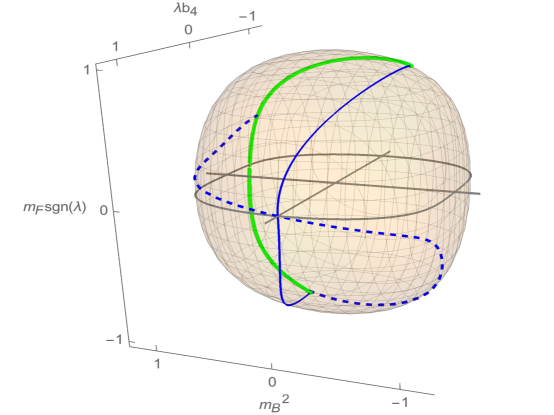
Figure 15: The phase diagram ellipsoid of the $\mathcal{N}=2$ theory for the value $|\lambda|=\tfrac{1}{4}$. The equator $m_{F}=0$ is displayed in gray. There are two solid and two dashed blue lines (one each in the northern hemisphere and one each in the southern hemisphere). The solid blue lines are described by CB conformal theories while the dashed blue lines are RF conformal theories – both correspond to second order phase transitions. The green line is a first order transition line and lies on the far side of the ellipsoid. The solid blue lines meet the green line at two points (one each on the two hemispheres) - these points are described by the RB conformal field theory. The solid blue (CB) and dashed blue (RF) lines meet at the point $(m_{B}^{2},\lambda b_{4},m_{F}\text{sgn}(\lambda))=(0,1,0)$ on the equator which is described by the CB-RF conformal field theory.

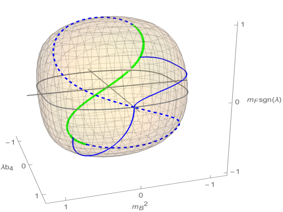
Figure 16: The phase diagram ellipsoid of the $\mathcal{N}=2$ theory for the value $|\lambda|=\tfrac{3}{4}$. The first order phase transition line in green is on the far side of the ellipsoid. Note that the first order line meets the dashed blue lines described by regular fermion CFTs. These meeting points themselves are described by critical fermion CFTs. The solid blue lines are described by critical boson CFTs and the intersection point of the two solid and two dashed blue lines is described by the CB-RF CFT. The features of this phase diagram can be obtained by applying the duality map (1) to the case $|\lambda|=\tfrac{1}{4}$.

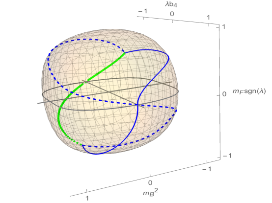
Figure 17: The phase diagram ellipsoid of the $\mathcal{N}=2$ theory for the value $|\lambda|=\tfrac{1}{2}$. The dashed blue lines are described by regular fermion CFTs and the solid blue lines are critical boson CFTs. The first order phase transition line in green is on the far side of the ellipsoid. Note that the first order line meets the dashed blue line and solid blue line at one point in the northern hemisphere and at one point in the southern hemisphere. These meeting points are presumably governed by a combination of critical fermion and regular boson CFTs i.e. an RB-CF CFT. The intersection point of the two solid and two dashed blue lines is described by the CB-RF CFT. The three special points, one on the equator, one in the northern hemisphere and one in the southern hemisphere are all expected to be described by CFTs that are self-dual under the duality (1).

Upto this point in this paper we have worked out the phase diagram of our theory only in the special case $|\lambda|<\frac{1}{2}$. The analysis for the case $|\lambda|>\frac{1}{2}$ proceeds in an entirely similar manner; the final results for this analysis could be anticipated from duality. We again give a three dimensional plot of the phase diagram for the representative value $|\lambda|=\tfrac{3}{4}$ in Figure 16.

Finally, we present the phase diagram for the case $|\lambda|=\tfrac{1}{2}$ in Figure 17 which is expected to be self-dual under the duality map (1). Note that the phase diagram in this case is very special. In particular, the line of second order CB phase transitions and the line of second order RF phase transitions end at a single critical point in each of the northern and southern hemisphere of phase diagram. The low energy dynamics of this critical point is presumably a theory of regular bosons and Gross-Neveu (or critical) fermions simultaneously interacting with a single $SU(N)$ Chern Simons gauge field at $|\lambda|=\frac{1}{2}$. This theory has never been studied before in the literature to the best of our knowledge, and there are several questions about it that would be interesting to investigate. In particular, this theory has four naively marginal operators. At first subleading order the coupling behind each of these terms will develop a $\beta$ function. It would be very interesting to study these $\beta$ functions and investigate the resultant structure of fixed points.

As we have mentioned above, moreover, $|\lambda|=\frac{1}{2}$ is special because this value is duality invariant. At precisely this value of $|\lambda|$, therefore, it should be possible to orbifold both the original UV theory (1) and the very special IR theory described in the previous paragraph by the duality operation (1). The resultant theory sounds particularly interesting to us because it is obtained by orbifolding with a Bose-Fermi duality: the excitations that survive this orbifolding are therefore maximally anyonic. The resultant theory should be simpler than its parent unorbifolded theory in some ways (for instance it will have only two rather than 4 naively marginal operators whose $\beta$ function we would have to control). It is conceivable that this orbifolded fixed point continues to exist at small finite values of $N$ and $k$ and could turn out to have applications in condensed matter physics. We feel that the detailed study of this theory is an interesting direction for future study.

5 The $\mathcal{N}=1$ locus

The class of theories (1) has a subset consisting of a two parameter set of ${\cal N}=1$ theories. The coupling constants in the Lagrangian are given in terms of the two parameters $\mu$ and $w$ as

$$m_{F}=\mu\ ,\ \ m_{B}^{2}=\mu^{2}\ ,\ \ b_{4}=\mu w\ ,\quad x_{4}=\frac{1+w}{2}\ ,\quad x_{6}=w^{2}-1\ ,\quad y_{4}^{\prime}=3+w\ ,\quad y_{4}^{\prime\prime}=w-1\ .$$ (88)

5.1 Classical analysis

From (1) one can read the classical potential for the field $\bar{\phi}\phi$ and the effective mass term for $\bar{\psi}\psi$ as

$$U_{\text{cl}}(\bar{\phi}\phi) =\kappa\left(m_{B}^{2}\frac{\bar{\phi}\phi}{\kappa}+4\pi b_{4}\left(\frac{\bar{\phi}\phi}{\kappa}\right)^{2}+4\pi^{2}(x_{6}+1)\left(\frac{\bar{\phi}\phi}{\kappa}\right)^{3}\right)+\left(4\pi x_{4}\frac{\bar{\phi}\phi}{\kappa}+m_{F}\right)\bar{\psi}\psi\ ,$$ (89)

which in the $\mathcal{N}=1$ theory becomes

$$U_{\text{cl}} ={\bar{\phi}\phi}\left(\mu+2\pi w\frac{\bar{\phi}\phi}{\kappa}\right)^{2}+\left(2\pi(1+w)\frac{\bar{\phi}\phi}{\kappa}+\mu\right)\bar{\psi}\psi\ .$$ (90)

The vacua of the above theory are characterised by $\phi=0$ and the following two possibilities for the scalar $\phi$:

$$\text{unHiggsed,}+:\quad\bar{\phi}\phi=0\ ,\qquad\text{Higgsed,}-:\quad 2\pi\bar{\phi}\phi=-\frac{\mu\kappa}{w}\ .$$ (91)

The condition $\text{sgn}(m_{F})\text{sgn}(\kappa)=\pm 1$ which decides the level of the low-energy Chern-Simons theories becomes

$$\pm:\qquad\text{sgn}(\kappa)\text{sgn}\left(\mu+2\pi(1+w)\frac{\bar{\phi}\phi}{\kappa}\right)=\pm 1\ ,$$ (92)

where $\bar{\phi}\phi$ has to be evaluated at one of the bosonic vacua in (91). The four possible phases $(\pm,\pm)$ are then characterised by

$$(+,+):\quad\bar{\phi}\phi=0\ ,\ \text{sgn}(\mu\kappa)=+1\ ,\qquad(+,-):\quad 2\pi\bar{\phi}\phi=-\frac{\mu\kappa}{w}\ ,\ \text{sgn}\left(-\frac{\mu\kappa}{w}\right)=+1\ ,$$

$$(-,+):\quad\bar{\phi}\phi=0\ ,\ \text{sgn}(\mu\kappa)=-1\ ,\qquad(-,-):\quad 2\pi\bar{\phi}\phi=-\frac{\mu\kappa}{w}\ ,\ \text{sgn}\left(-\frac{\mu\kappa}{w}\right)=-1\ .$$ (93)

Classically, we need to satisfy ${\bar{\phi}}\phi\geq 0$ and we see that this is possible in the $(+,+)$, $(-,+)$, $(+,-)$ phases for appropriate choices of signs of $\mu$, $w$ and $k$. However ${\bar{\phi}}\phi$ is required to be negative in the $(-,-)$ phase which is impossible classically. Thus, the $\mathcal{N}=1$ theory never has a classical vacuum in this phase.

5.2 At finite $\lambda$

Recall that the large $N$ analysis provides us with an exact (i.e. to all orders in $\lambda$) Landau-Ginzburg effective potential for the theory for the variable $\sigma$ (in fact, for the variable $(\bar{\phi}\phi)_{\rm cl}$ which is related to $\sigma$ via (30)). The phases are determined by the minima of the Landau-Ginzburg potential. The four phases are characterised in terms of the minimum value of $\sigma$ as (cf. (2.5) and (2.5))

$$(+,+):\quad\text{sgn}(1+w)\sigma>-\frac{\mu}{\lambda}\frac{1}{|1+w|}\ ,\qquad \sigma<0\ ,$$

$$(+,-):\quad\text{sgn}(1+w)\sigma>-\frac{\mu}{\lambda}\frac{1}{|1+w|}\ ,\qquad \sigma>0\ ,$$

$$(-,+):\quad\text{sgn}(1+w)\sigma<-\frac{\mu}{\lambda}\frac{1}{|1+w|}\ ,\qquad \sigma<0\ ,$$

$$(-,-):\quad\text{sgn}(1+w)\sigma<-\frac{\mu}{\lambda}\frac{1}{|1+w|}\ ,\qquad \sigma>0\ .$$ (94)

For any given set of values for the signs $\text{sgn}(1+w)$ and $\text{sgn}(\mu)\text{sgn}(\lambda)$, the potential explores three among the four phases above as given in Figure 3. We reproduce this figure in terms of the variables $\mu$, $\lambda$ and $w$ in Figure 18 for easy reference.

Figure 18: Regions of validity for different branches of the potential for various choices of $\text{sgn}(\mu)\text{sgn}(\lambda)$ and $\text{sgn}(1+w)$.

Plugging in the special locus of values (88) in the general expression for the Landau-Ginzburg potential in (45), we get

$$U^{(\varepsilon,\pm)}(\sigma)=\frac{N}{2\pi}\Big{[}\left(w^{2}-1-\phi_{\pm}+\tfrac{1}{8}(1+w)^{3}\psi_{\varepsilon}\right)\lambda^{2}{\sigma}^{3}+\\ \left(w+\tfrac{3}{16}(1+w)^{2}\psi_{\varepsilon}\right)2\mu\lambda{\sigma}^{2}+\left(1+\tfrac{3}{8}(1+w)\psi_{\varepsilon}\right)\mu^{2}{\sigma}+\tfrac{1}{8\lambda}\psi_{\varepsilon}\mu^{3}\Big{]}\ .$$ (95)

where as earlier, $\varepsilon=\pm$ denotes the fermionic phases and the explicit $\pm$ denotes the bosonic phases.

It turns out that, on the $\mathcal{N}=1$ locus of parameters, the Landau-Ginzburg potential in each of the four branches can be written in a very specific form:

$$U_{\text{eff}}^{({\rm+,+})}(\sigma) =\frac{N}{2\pi}\frac{\lambda^{2}\psi_{+}}{8}(w-a_{1})^{2}(w-c_{1})\times\left(\sigma+\frac{\mu}{\lambda}\frac{1}{w-a_{1}}\right)^{2}\left(\sigma+\frac{\mu}{\lambda}\frac{1}{w-c_{1}}\right)\ ,$$

$$U_{\text{eff}}^{({\rm+,-})}(\sigma) =\frac{N}{2\pi}\frac{\lambda^{2}\psi_{+}}{8}(w-a_{2})^{2}(w-c_{2})\times\left(\sigma+\frac{\mu}{\lambda}\frac{1}{w-a_{2}}\right)^{2}\left(\sigma+\frac{\mu}{\lambda}\frac{1}{w-c_{2}}\right)\ ,$$

$$U_{\text{eff}}^{({\rm-,+})}(\sigma) =\frac{N}{2\pi}\frac{\lambda^{2}\psi_{-}}{8}(w-a_{3})^{2}(w-c_{3})\times\left(\sigma+\frac{\mu}{\lambda}\frac{1}{w-a_{3}}\right)^{2}\left(\sigma+\frac{\mu}{\lambda}\frac{1}{w-c_{3}}\right)\ ,$$

$$U_{\text{eff}}^{({\rm-,-})}(\sigma) =\frac{N}{2\pi}\frac{\lambda^{2}\psi_{-}}{8}(w-a_{4})^{2}(w-c_{4})\times\left(\sigma+\frac{\mu}{\lambda}\frac{1}{w-a_{4}}\right)^{2}\left(\sigma+\frac{\mu}{\lambda}\frac{1}{w-c_{4}}\right)$$

$$\quad-\frac{N}{2\pi}\frac{32|\lambda|^{3}}{3(4-|\lambda|^{2})^{2}}\sigma^{3}\ ,$$ (96)

where $\psi_{\pm}$ are defined in (43) and $a_{i}$ and $c_{i}$ are the following functions of $|\lambda|$:

$$a_{1} =-\frac{2-|\lambda|}{|\lambda|}\ ,\quad a_{2}=\frac{1}{a_{1}}\ ,\quad c_{1}=\frac{2-2|\lambda|-|\lambda|^{2}}{|\lambda|(2-|\lambda|)}\ ,\quad c_{2}=-\frac{6-6|\lambda|+|\lambda|^{2}}{|\lambda|(2-|\lambda|)}\ ,$$

$$a_{3} =\frac{2+|\lambda|}{|\lambda|}\ ,\quad a_{4}=\frac{1}{a_{3}}\ ,\quad c_{3}=-\frac{2+2|\lambda|-|\lambda|^{2}}{|\lambda|(2+|\lambda|)}\ ,\quad c_{4}=\frac{|\lambda|^{2}+6|\lambda|+6}{|\lambda|(2+|\lambda|)}\ .$$ (97)

We give the locations of the quantities $a_{1}$, $a_{2}$, $a_{3}$, $c_{1}$, $c_{2}$, $c_{3}$ on the $w$-line in Figure 19 since they clearly signify special points for the potential above. The ordering of these quantities shown in Figure 19 holds for any value of $|\lambda|$ between $0$ and $1$.

Figure 19: Locations of the various functions of $|\lambda|$ in (5.2) on the $w$-line for all values of $|\lambda|$.

The first three potentials are of the form

$$U(\sigma)=\frac{N}{2\pi}\frac{\lambda^{2}\psi}{8}(w-a)^{2}(w-c)\left(\sigma+\frac{\mu}{\lambda}\frac{1}{w-a}\right)^{2}\left(\sigma+\frac{\mu}{\lambda}\frac{1}{w-c}\right)\ ,$$ (98)

whereas the potential for the $(-,-)$ branch fails to be of the above form due to the additional term proportional to $\sigma^{3}$. We analyse the $(+,+)$, $(+,-)$ and $(-,+)$ branches first by studying the function in (98) above and then study the $(-,-)$ branch separately.

To begin with, we analyse the function (98) when $w\neq a,c$. The function (98) has zeroes at

$$\sigma=-\frac{\mu}{\lambda}\frac{1}{w-a}\ ,-\frac{\mu}{\lambda}\frac{1}{w-a}\ ,-\frac{\mu}{\lambda}\frac{1}{w-c}\ .$$ (99)

Since there is a double zero at $\sigma=-\frac{\mu}{\lambda}\frac{1}{w-a}$, this zero is also an extremum of the potential. It is a minimum when

$$\psi\frac{\mu}{\lambda}\left(\frac{c-a}{w-a}\right)>0\ .$$ (100)

The other extremum of the potential lies between the two zeroes at

$$\sigma=-\frac{\mu}{3\lambda}\left(\frac{2}{w-c}+\frac{1}{w-a}\right)\ .$$ (101)

Based on these facts and the ordering of the $a_{i}$ and $c_{i}$ in Figure 19, the profile of the potential can be deduced in the $(+,+)$, $(+,-)$ and $(-,+)$ branches listed in (5.2). We have displayed the result of such an analysis in Figure 20, 21 and 21 for the $(+,+)$, $(+,-)$ and $(-,+)$ branches respectively.

Note that there are special values of $w$ viz. $w=a,c$ where the form of the function (98) changes from being cubic to being either quadratic or linear in $\sigma$. When $w=a$, we have

$$U(\sigma)\Big{|}_{w=a}=\frac{N}{2\pi}\frac{\mu^{2}\psi}{8}(a-c)\left(\sigma+\frac{\mu}{\lambda}\frac{1}{a-c}\right)\ ,$$ (102)

It is easy to see that when $w$ approaches $a$, the double zero (hence also an extremum) at $\sigma=-\frac{\mu}{\lambda}\frac{1}{w-a}$ and the other extremum (101) both go away to $\sigma=\pm\infty$ and the potential becomes linear. More specifically, let us start with a value of $w$ just below $a$. As $w$ is increased towards $a$ the extremum listed in the first of (99) and the extremum listed in (101) both move towards $\text{sgn}(\mu\lambda)\infty$. As $w$ is increased above $a$, these two extrema reappear, but this time at $-\text{sgn}(\mu\lambda)\infty$.

When $w=c$, we have

$$U(\sigma)\Big{|}_{w=c}=\frac{N}{2\pi}\frac{\mu\lambda\psi}{8}(a-c)^{2}\left(\sigma+\frac{\mu}{\lambda}\frac{1}{c-a}\right)^{2}\ ,$$ (103)

Again, it is easy to see that as one approaches $w=c$ from below the single zero $\sigma=-\frac{\mu}{\lambda}\frac{1}{w-c}$ and the extremum (101) go away to $\text{sgn}(\mu\lambda)\infty$ (the double zero in (99) survives and becomes the extremum of the quadratic potential (103) above). When $w$ is just larger than $c$ both the zero and the extremum which disappeared at $w=c$ reappaer at $\sigma=-\text{sgn}(\mu\lambda)\infty$.

Figure 20: Profile of the function $U_{\rm eff}^{(+,+)}(\sigma)$ as $w$ (horizontal line in this graph) runs from $-\infty$ to $\infty$. The vertical line in each potential plot with label $0$ denotes the point $\sigma=0$ and the unlabelled vertical line is the point $\sigma=-\frac{\mu}{\lambda}\frac{1}{1+w}$.

Figure 21: Profile of the function $U_{\rm eff}^{(+,-)}(\sigma)$ as $w$ (horizontal line in this graph) runs from $-\infty$ to $\infty$. The vertical line in each potential plot with label $0$ denotes the point $\sigma=0$ and the unlabelled vertical line is the point $\sigma=-\frac{\mu}{\lambda}\frac{1}{1+w}$.

Figure 22: Profile of the function $U_{\rm eff}^{(-,+)}(\sigma)$ as $w$ (horizontal line in this graph) runs from $-\infty$ to $\infty$. The vertical line in each potential plot with label $0$ denotes the point $\sigma=0$ and the unlabelled vertical line is the point $\sigma=-\frac{\mu}{\lambda}\frac{1}{1+w}$.

The $(-,-)$ branch potential is not completely of the form (98). There is an additional cubic term in $\sigma$ which changes the behaviour quite drastically. In fact, it can be easily verified that the cubic potential on the $(-,-)$ branch always has three real zeroes and (hence) none of these zeroes are extrema of the potential. We do not give all the cumbersome details of the potential for different values of $w$ and only plot the appropriate part of the potential on the $(-,-)$ branch wherever it is required for the analysis of the vacuum structure below.

Note that in the first three branches in (5.2), the form of the potential (98) closely mirrors that of the tree-level potential (90). We reproduce below the tree-level potential in terms of the variable $\sigma$

$$U_{\text{cl}}(\sigma) =\frac{N}{2\pi}\sigma\times\lambda^{2}w^{2}\left(\sigma+\frac{\mu}{\lambda}\frac{1}{w}\right)^{2}\ .$$ (104)

The specific form of the classical potential is not an accident and is in fact due to $\mathcal{N}=1$ supersymmetry. The potential energy density for an $\mathcal{N}=1$ supersymmetric theory with a scalar superfield $\phi$ with the usual superspace kinetic term for $\phi$ and a superspace potential term $W(\phi,\bar{\phi})$ is of the form

$$\bar{\phi}\phi\left|\frac{\partial W}{\partial\phi}\right|^{2}\ .$$ (105)

In particular, note that the potential above is the product of a positive definite term $\bar{\phi}\phi$ that comes from the kinetic term and another positive definite term $|W^{\prime}|^{2}$ that comes from the superspace potential term. The Landau-Ginzburg potential for the branches $(+,+)$, $(+,-)$ and $(-,+)$ is also precisely of this form:

$$U_{\text{qu}}(\sigma) =\frac{N}{2\pi}\frac{\psi_{\pm}}{8}(w-c)\left(\sigma+\frac{\mu}{\lambda}\frac{1}{w-c}\right)\times\lambda^{2}(w-a)^{2}\left(\sigma+\frac{\mu}{\lambda}\frac{1}{w-a}\right)^{2}\ .$$ (106)

The first factor above is linear in $\sigma$ and is a $\lambda$-dependent deformation of the $\sigma$ factor in the classical potential. It can be easily checked that this factor is positive definite in the domain of validity in $\sigma$ of the appropriate branch (one of $(+,+)$, $(+,-)$, $(-,+)$) of the potential. Given the comparison with the classical potential it is tempting to conjecture that this factor arises from the superspace kinetic term of appropriate scalar superfield whose bosonic component involves $\sigma$. The second factor is the square of a term linear in $\sigma$ and is again a $\lambda$-dependent deformation of the $|W^{\prime}|^{2}$ term in the classical potential. Presumably, this complete square term arises from an appropriate superspace potential for the same superfield whose bosonic component involves $\sigma$. Note that the potential on the $(-,-)$ branch is not of this form and this may be tied to the fact that a classical supersymmetric vacuum does not exist in the $(-,-)$ branch.

5.3 The vacuum structure

We study the exact Landau-Ginzburg potential for the $\mathcal{N}=1$ theory at different values of $w$. The regions of validity of the different branches of the potential are given in Figure 18 for different values of $\text{sgn}(\mu\lambda)$ and $\text{sgn}(1+w)$. We borrow the appropriate parts of the potential for the $(+,+)$, $(+,-)$ and $(-,+)$ branches from Figures 20, 21, 22 and separately plot the $(-,-)$ branch wherever required, and patch them together to obtain the Landau-Ginzburg potential. We provide a representative plot of the potential for each interval in the $w$-line displayed in Figure 19. We only indicate those special values of $w$ where the phase structure of the potential changes and hide the remaining values in order to avoid cluttering.

As is apparent from Figure 18, it is useful to separate the two cases $\text{sgn}(\mu)\text{sgn}(\lambda)=\pm 1$. We display the potential for different values of $w$ in Figure 23 for $\text{sgn}(\mu)=\text{sgn}(\lambda)$ and in Figure 24 for $\text{sgn}(\mu)=-\text{sgn}(\lambda)$. We explain briefly the features of Figures 23 and 24. Firstly, note that as $w$ crosses the special value $-1$ the various branches among $(\pm,\pm)$ that the Landau-Ginzburg potential accesses changes. Next, note that the $(-,-)$ that appears for $\mu\lambda<0$ never has a minimum in it. As $w$ crosses one of $a_{1}$, $a_{2}$ or $a_{3}$, new vacua appear from infinity or already-existing vacua disappear to infinity in the $(+,+)$, $(+,-)$ or $(-,+)$ branches respectively. This is due to the potential becoming linear from being cubic in the branch in which the vacuum structure changes, as explained in detail around (102).

Figure 23: The Landau-Ginzburg potential $U_{\rm eff}(\sigma)$ plotted for $w$ (horizontal line in this graph) ranging from $-\infty$ to $\infty$, in the case that $\text{sgn}(\mu)=\text{sgn}(\lambda)$. One of the two vertical lines in each plot of $U_{\rm eff}(\sigma)$ - the line that separates a bosonic (second index) $+$ phase from a bosonic $-$ phase - lies at $\sigma=0$. The second vertical line separates the fermionic (first index) $+$ phase from the fermionic $-$ phase and lies at $\sigma=-\frac{\mu}{\lambda}\frac{1}{1+w}$ and occurs at either positive or negative values of $\sigma$ depending on the value of $w$. The brackets below the horizontal line denote the phase(s) of the theory for the appropriate ranges of $w$. The quantities $a_{1}$, $a_{2}$ and $a_{3}$ are defined in (5.2) and are given by $a_{1}=a_{2}^{-1}=-\frac{2-|\lambda}{|\lambda|}$, $a_{3}=\frac{2+|\lambda|}{|\lambda|}$.

Figure 24: The Landau-Ginzburg potential $U_{\rm eff}(\sigma)$ plotted for values of the parameter $w$ (horizontal line in this graph) ranging from $-\infty$ to $\infty$ in the case that $\text{sgn}(\mu)=-\text{sgn}(\lambda)$. We follow the same notation as in Figure 23.

5.4 Quantum versus Classical

In the classical limit $|\lambda|\to 0$ the vacuum structure of the ${\cal N}=1$ theory simplifies. In this limit $a_{1}$ and $a_{3}$ in Fig 23 and Figure 24 respectively tend to $-\infty$ and $+\infty$. It follows that in this limit we have either one or two vacua depending on whether $\mu\lambda w>0$ or $\mu\lambda w<0$, in agreement with the result of the classical analysis in Section 5.1.

Let us now consider the case $\lambda\neq 0$ but $\lambda$ small. In this case the quantum vacuum (or phase) structure agrees with the classical vacuum structure at values of $w$ that are order unity, but differs from the classical result when $w$ is of order $\frac{1}{\lambda}$. In more detail, let us first consider the case $\lambda\mu>0$, depicted in Figure 23. In this case we have two classical vacua - one at $\sigma=0$ and one at $\sigma>0$ - when $w<0$, but only one such vacuum (at $\sigma=0$) when $w>0$. As mentioned above, this result continues to hold in the quantum case when $w$ is of order unity. Let us now follow the fate of these ‘classical’ vacua (i.e vacua that have a clear classical counterpart) as $|w|$ is increased to order $1/\lambda$. When $w$ is taken large and positive, for $w>a_{3}$ we find that the single classical vacuum at $\sigma<0$ splits up into two vacua, both at $\sigma<0$ (see Fig 23). The extra vacuum comes in from infinity when $w$ crosses $a_{3}$. On the other hand when $w$ is taken so large and negative that $w<a_{1}$ we find that one of the vacua (the unHiggsed vacuum, namely the continuation of the classical vacuum at $\phi=0$) goes away to infinity. In this range the quantum theory has only one vacuum - the Higgsed vacuum. Thus we see that quantum effects, when sufficiently strong, lead to new vacua coming in from infinity as well as vacua going away to infinity, including those that exist classically. Clearly this phenomenon is non-perturbative (as it happens at values of $w$ of order $1/\lambda$).

The situation is ‘reversed’ when $\mu\lambda<0$. In this case the single classical vacuum (the unHiggsed vacuum) that existed for $w<0$ splits into two unHiggsed vacua when $w<a_{1}$ (i.e. one extra vacuum comes in from infinity in the unHiggsed phase of the boson), while the unHiggsed vacuum (one of the two vacua that exist for $w>0$ in the classical limit) goes away to infinity when $w>a_{3}$.

We find the fact that we can reliably track the non-perturbative appearance and disappearance of supersymmetric vacua as a function of $w$ quite remarkable. It is important, however, to remember that we only have the ability to vary $w$ continuously in the strict large $N$ limit. At any finite value of $N$, the parameter $w$ will be forced to lie at a one of discrete set of points (an issue investigated in some detail in the soon-to-appear paper ofer ), and so cannot be varied continuously.

6 Acknowledgements

We would like to thank O. Aharony, F. Benini, L. Janagal, A. Mishra, D. Radicevic and A. Sharon for useful discussions. We would also like to thank O. Aharony and A. Sharon for sharing an advance version of their draft ofer with us. The work of A. D., I. H., S. M., and N. P. was supported by the Infosys Endowment for the study of the Quantum Structure of Spacetime. S. J. would like to thank TIFR, Mumbai for hospitality during the completion of this work. The work of S. J. is supported by the Ramanujan Fellowship. Finally we would all like to acknowledge our debt to the steady support of the people of India for research in the basic sciences.

Appendix A A review of the critical fermion and regular boson theories and their zero-temperature phase diagrams

The regular boson (RB) theory is defined by the action

$$S_{\rm RB} =\int d^{3}x\biggl{[}\frac{i\kappa_{B}}{4\pi}\varepsilon^{\mu\nu\rho}\mathrm{Tr}(X_{\mu}\partial_{\nu}X_{\rho}-\tfrac{2i}{3}X_{\mu}X_{\nu}X_{\rho})+D_{\mu}\bar{\phi}D^{\mu}\phi$$

$$\qquad\qquad\quad+m_{B}^{2}\bar{\phi}\phi+\frac{4\pi{b}_{4}}{\kappa_{B}}(\bar{\phi}\phi)^{2}+\frac{4\pi^{2}}{\kappa_{B}^{2}}\left(x^{B}_{6}+1\right)(\bar{\phi}\phi)^{3}\biggl{]}\ ,$$ (107)

while the following action defines the critical fermion (CF) theory

$$S_{\rm CF} =\int d^{3}x\bigg{[}\frac{i\kappa_{F}}{4\pi}\varepsilon^{\mu\nu\rho}\mathrm{Tr}(X_{\mu}\partial_{\nu}X_{\rho}-\tfrac{2i}{3}X_{\mu}X_{\nu}X_{\rho})+\bar{\psi}\gamma_{\mu}D^{\mu}\psi$$

$$\qquad\qquad\quad-\frac{4\pi}{\kappa_{F}}\zeta_{F}\left(\bar{\psi}\psi-\frac{\kappa_{F}y_{2}^{2}}{4\pi}\right)-\frac{4\pi y_{4}}{\kappa_{F}}\zeta_{F}^{2}+\frac{4\pi^{2}}{\kappa_{F}^{2}}x_{6}^{F}\zeta_{F}^{3}\bigg{]}\ .$$ (108)

where

$$\kappa_{B}={\text{sgn}}(k_{B})\left(|k_{B}|+N_{B}\right)\ ,\quad\kappa_{F}={\text{sgn}}(k_{F})\left(|k_{F}|+N_{F}\right)\ ,$$ (109)

are the renormalized Chern-Simons levels and $k_{F}$ and $k_{B}$ are the levels of the WZW theory dual to the pure Chern-Simons theory. These two theories are conjectured to be dual to each other under the following map between the various parameters appearing in the Lagrangians (107), (A):

$$\kappa_{B}=-\kappa_{F}\ ,\quad N_{B}=|k_{F}|\ ,\quad x_{6}^{F}=x_{6}^{B}\ ,\quad y_{4}={b}_{4}\ ,\quad y_{2}^{2}=m_{B}^{2}\ .$$ (110)

The theories can be solved exactly in the large $N$ limit by a saddle-point computation. For instance, the thermal free energies have been computed to all orders in the ’t Hooft coupling $\lambda=N/k$. Further, the same computation yields equations for the pole masses $c_{B}$ and $c_{F}$ of the RB and CF theories, as well as the equations governing the vacuum expectation value of the gauge invariant operator $\bar{\phi}\phi$ in the RB theory and the operator $\zeta_{F}$ in the CF theory. The thermal free energies and the equations for the pole masses and vev’s map to each other under the duality map (110).

In a previous paper Dey:2018ykx , a three variable off-shell generalisation of the thermal free energy of the RB (CF) theory was presented, which upon extremization with respect to its three variables, yielded the saddle-point equations for the pole mass $c_{B}$ ($c_{F}$) and the vev of $\bar{\phi}\phi$ ($\zeta_{F}$). We present this off-shell generalisation below, and the corresponding saddle-point equations for the regular boson theory first.

A.1 The regular boson theory

A.1.1 The thermal free energy

We define the variable $\sigma_{B}$ as short-hand for the vacuum expectation value of the operator $\bar{\phi}\phi$:

$$\sigma_{B}=\frac{2\pi}{N_{B}}\langle\bar{\phi}\phi\rangle\ .$$ (111)

The three-variable off-shell free energy for the regular boson theory is then given by (see equation (4.2) of Dey:2018ykx ),

$$F(c_{B},\sigma_{B},\tilde{{\cal S}})$$

$$=\frac{N_{B}}{6\pi}\Bigg{[}-3{\hat{c}}_{B}^{2}{\hat{\sigma}}_{B}+\lambda_{B}^{2}{\hat{\sigma}}_{B}^{3}+3\left({\hat{m}}_{B}^{2}{\hat{\sigma}}_{B}+2\lambda_{B}{\hat{b}}_{4}{\hat{\sigma}}_{B}^{2}+(x_{6}+1)\lambda_{B}^{2}{\hat{\sigma}}_{B}^{3}\right)$$

$$\qquad\qquad-4\lambda_{B}^{2}({\tilde{{\cal S}}}+{\hat{\sigma}}_{B})^{3}+6|\lambda_{B}|{\hat{c}}_{B}({\tilde{{\cal S}}}+{\hat{\sigma}}_{B})^{2}$$

$$\qquad\qquad-{\hat{c}}_{B}^{3}+3\int_{-\pi}^{\pi}d\alpha\,\rho_{B}(\alpha)\,\int_{{\hat{c}}_{B}}^{\infty}dy~{}y~{}\left(\ln\left(1-e^{-y-i\alpha}\right)+\ln\left(1-e^{-y+i\alpha}\right)\right)\Bigg{]}\ ,$$ (112)

where $\rho_{B}(\alpha)$ is the distribution function for the holonomy $\alpha$ of the $SU(N)$ gauge field around the thermal circle. The last line in (A.1.1) arises from the one-loop determinant of the fundamental bosonic field.

Note that (A.1.1) is a function of three ‘field’ variables, namely $c_{B}$, $\sigma_{B}$ and ${\tilde{\cal S}}$ (the hats on some of the variables indicate that they have been scaled by appropriate powers of the temperature to make them dimensionless). We use the same notation for the off-shell variables $c_{B}$ and $\sigma_{B}$ and their saddle-point values which are the pole mass of the fundamental bosonic excitation and the vacuum expectation value (111) respectively. We do not have a physical interpretation of the variable ${\tilde{{\cal S}}}$ but, as we shall see below, it becomes the following function of the pole mass $c_{B}$ on-shell:

$${\cal S}(c_{B})=\frac{1}{2}\int_{-\pi}^{\pi}d\alpha\,\rho_{B}(\alpha)\left(\log(2\sinh(\tfrac{\hat{c}_{B}+i\alpha}{2}))+\log(2\sinh(\tfrac{\hat{c}_{B}-i\alpha}{2}))\right)\ ,$$ (113)

Extremizing (A.1.1) w.r.t. ${\tilde{\cal S}}$, $c_{B}$ and $\sigma_{B}$ respectively yields the equations (see equation (4.3) of Dey:2018ykx )

$$({\tilde{\cal S}}+{\hat{\sigma}}_{B})(-{\hat{c}}_{B}+|\lambda_{B}|({\tilde{\cal S}}+{\hat{\sigma}}_{B}))=0\ ,$$

$${\hat{c}}_{B}({\cal S}(c_{B})+{\hat{\sigma}}_{B})-|\lambda_{B}|({\tilde{\cal S}}+{\hat{\sigma}}_{B})^{2}=0\ ,$$

$${\hat{c}}_{B}^{2}-{\hat{m}}_{B}^{2}-4{\hat{c}}_{B}|\lambda_{B}|({\tilde{\cal S}}+{\hat{\sigma}}_{B})+\lambda_{B}\left(4{\tilde{\cal S}}^{2}\lambda_{B}-4{\hat{b}}_{4}{\hat{\sigma}}_{B}+8\lambda_{B}{\hat{\sigma}}_{B}{\tilde{\cal S}}-3\lambda_{B}{\hat{\sigma}}_{B}^{2}x_{6}^{B}\right)=0\ .$$ (114)

The first equation offers us a choice between two solutions:

$$\text{unHiggsed}(\text{uH}): \quad{\tilde{{\cal S}}}=-{\hat{\sigma}}_{B}\ ,$$

$$\text{Higgsed}(\text{H}): \quad{\tilde{{\cal S}}}=\frac{{\hat{c}}_{B}}{|\lambda_{B}|}-{\hat{\sigma}}_{B}\ .$$ (115)

Substituting either of the two solutions for ${\tilde{{\cal S}}}$ above into the second equation of (A.1.1) gives ${\tilde{{\cal S}}}={\cal S}(c_{B})$ on-shell as claimed earlier. More importantly, we get two expressions for the thermal free energy as a function of two variables $c_{B}$ and $\sigma_{B}$:

$$F^{\rm(uH)}(c_{B},\sigma_{B}) =\frac{N_{B}}{2\pi}\Bigg{[}-\frac{1}{3}{\hat{c}}_{B}^{3}-{\hat{c}}_{B}^{2}{\hat{\sigma}}_{B}+{\hat{m}}_{B}^{2}{\hat{\sigma}}_{B}+2\lambda_{B}{\hat{b}}_{4}{\hat{\sigma}}_{B}^{2}+(\tfrac{4}{3}+x_{6}^{B})\lambda_{B}^{2}{\hat{\sigma}}_{B}^{3}$$

$$\qquad\qquad+\int_{-\pi}^{\pi}d\alpha\,\rho_{B}(\alpha)\,\int_{{\hat{c}}_{B}}^{\infty}dy\,y\,\left(\ln\left(1-e^{-y-i\alpha}\right)+\ln\left(1-e^{-y+i\alpha}\right)\right)\Bigg{]}\ ,$$

$$F^{\rm(H)}(c_{B},\sigma_{B}) =\frac{N_{B}}{2\pi}\Bigg{[}-\frac{|\lambda_{B}|-2}{3|\lambda_{B}|}{\hat{c}}_{B}^{3}-{\hat{c}}_{B}^{2}{\hat{\sigma}}_{B}+{\hat{m}}_{B}^{2}{\hat{\sigma}}_{B}+2\lambda_{B}{\hat{b}}_{4}{\hat{\sigma}}_{B}^{2}+(\tfrac{4}{3}+x_{6}^{B})\lambda_{B}^{2}{\hat{\sigma}}_{B}^{3}$$

$$\qquad\qquad+\int_{-\pi}^{\pi}d\alpha\,\rho_{B}(\alpha)\,\int_{{\hat{c}}_{B}}^{\infty}dy\,y\,\left(\ln\left(1-e^{-y-i\alpha}\right)+\ln\left(1-e^{-y+i\alpha}\right)\right)\Bigg{]}\ .$$ (116)

The interpretation of the two branches of solution in (A.1.1) (and consequently the two branches of free energy) is that one of them corresponds to the unHiggsed phase and the other corresponds to the Higgsed phase. By comparing with direct computations of the free energies in both the phases (Aharony:2012ns ; Jain:2013py for the unHiggsed phase and Dey:2018ykx for the Higgsed phase), we observe that the first equation in (A.1.1) corresponds to the unHiggsed phase and the second to the Higgsed phase.

Extremizing the expressions in (A.1.1) w.r.t. $c_{B}$ gives the equations for $\sigma_{B}$ in (A.1.1) with ${\tilde{{\cal S}}}$ replaced by its on-shell value ${\cal S}(c_{B})$:

$$\text{unHiggsed}: \quad{\hat{\sigma}}_{B}=-{\cal S}(c_{B})\ ,$$

$$\text{Higgsed}: \quad{\hat{\sigma}}_{B}=\frac{{\hat{c}}_{B}}{|\lambda_{B}|}-{{\cal S}}(c_{B})\ .$$ (117)

Extremizing (A.1.1) w.r.t. $\sigma_{B}$ gives the following equations for $c_{B}$ which are the equations for the pole mass of the fundamental bosonic excitation in the respective phases:

$$\text{unHiggsed}: \quad{\hat{c}}_{B}^{2}-{\hat{m}}_{B}^{2}+4{\hat{b}}_{4}\lambda_{B}{\cal S}-(4+3x_{6}^{B})\lambda_{B}^{2}{\cal S}^{2}=0\ ,$$

$$\text{Higgsed}: \quad{\hat{c}}_{B}^{2}-{\hat{m}}_{B}^{2}+4{\hat{b}}_{4}(\lambda_{B}{\cal S}-\text{sgn}(\lambda_{B}){\hat{c}}_{B})-(4+3x_{6}^{B})(\lambda_{B}{\cal S}-\text{sgn}(\lambda_{B}){\hat{c}}_{B})^{2}=0\ .$$ (118)

Solving the theory then amounts to solving the above equations for $c_{B}$ in the respective phases and plugging back into (A.1.1) to obtain the corresponding values of $\sigma_{B}$. Once we have the values of $c_{B}$ and $\sigma_{B}$, we plug them into the free energy expressions in (A.1.1) to obtain the on-shell thermal free energies in the two phases.

A.1.2 The zero temperature LG potential

At zero temperature, the free energies and saddle-point equations becomes very simple. The simplifications are as follows:

1. The term with the integral over $y$ in the second line of the free energy expressions vanishes.

2. The quantity ${\cal S}(c_{B})$ simplifies to

   $${\cal S}(c_{B})=\frac{{\hat{c}}_{B}}{2}\ ,$$ (119)

   which in turn simplifies the equations (A.1.1):

   $$\text{unHiggsed}: \quad{\sigma}_{B}=-\frac{c_{B}}{2}\ ,$$

   $$\text{Higgsed}: \quad{\sigma}_{B}=\frac{{c}_{B}}{|\lambda_{B}|}-\frac{c_{B}}{2}\ ,$$ (120)

   and equations (A.1.1):

   $$\text{unHiggsed}: \quad\left(1-\lambda_{B}^{2}(1+\tfrac{3}{4}x_{6}^{B})\right){c}_{B}^{2}-2\lambda_{B}{b}_{4}c_{B}-{m}_{B}^{2}=0\ ,$$

   $$\text{Higgsed}: \quad\left(1-\left(\tfrac{2-|\lambda_{B}|}{2|\lambda_{B}|}\right)^{2}\lambda_{B}^{2}(1+\tfrac{3}{4}x_{6}^{B})\right){c}_{B}^{2}-2\lambda_{B}{b}_{4}\left(\tfrac{2-|\lambda_{B}|}{|\lambda_{B}|}\right)c_{B}-{m}_{B}^{2}=0\ .$$ (121)

   Thus, the quadratic equation (2) determines the pole mass $c_{B}$ and the linear equation (2) determines the vacuum expectation value $\sigma_{B}$.

3. As a consequence of (2) we see that $\sigma_{B}$ can assume only negative values in the unHiggsed phase and only positive values in the Higgsed phase since $c_{B}$ is by definition a positive quantity.

It is useful and conceptually attractive to rewrite the zero temperature limit of the two-variable free energy (A.1.1) in terms of $\sigma_{B}$ alone using the simple relations (2) between $c_{B}$ and $\sigma_{B}$. As one can see from the expressions in (A.1.1), this changes the coefficient of the $\sigma_{B}^{3}$ term in the free energy.

The resulting function of $\sigma_{B}$ is precisely the quantum effective potential for the field $(\bar{\phi}\phi)_{\rm cl}$ corresponding to the expectation value of the gauge invariant operator $\bar{\phi}\phi$ (cf. Section 2.4 in the main text). The effective potential turns out to be (see equation (5.10) in Dey:2018ykx )

$$U_{\rm RB}(\sigma_{B})=\left\{\begin{array}[]{cl}\displaystyle\frac{N_{B}}{2\pi}\left[(x_{6}^{B}-\phi_{+})\lambda_{B}^{2}{\sigma}_{B}^{3}+2\lambda_{B}b_{4}{\sigma}_{B}^{2}+m_{B}^{2}{\sigma}_{B}\right]&\quad\text{for }\sigma_{B}<0\ ,\\ \displaystyle\frac{N_{B}}{2\pi}\left[(x_{6}^{B}-\phi_{-})\lambda_{B}^{2}{\sigma}_{B}^{3}+2\lambda_{B}{b}_{4}{\sigma}_{B}^{2}+{m}_{B}^{2}{\sigma}_{B}\right]&\quad\text{for }\sigma_{B}>0\ ,\end{array}\right.$$ (124)

where $\phi_{\pm}$ are the following functions of $|\lambda_{B}|$:

$$\phi_{+}=\frac{4}{3}\left(\frac{1}{|\lambda_{B}|^{2}}-1\right)\ ,\quad\phi_{-}=\frac{4}{3}\left(\frac{1}{(2-|\lambda_{B}|)^{2}}-1\right)\ ,$$ (125)

with the ordering $\phi_{-}<0<\phi_{+}$ for all values of $|\lambda_{B}|$. These functions are referred to as $\phi_{1}$ and $\phi_{2}$ respectively in the earlier work Aharony:2018pjn ; Dey:2018ykx . The solutions of the saddle-point equations (2) and (2) can then be phrased as the problem of minimisation of the quantum effective potential $U_{\rm RB}(\sigma_{B})$.

A.1.3 Stability of the regular boson theory

The stability of the regular boson theory can be studied very easily using the effective potential in (124). The potential is stable (meaning, it increases without bound as $|\sigma_{B}|$ increases) when the marginal (at large $N_{B}$) parameter $x_{6}^{B}$ satisfies the following bound

$$\phi_{-}<x_{6}^{B}<\phi_{+}\ .$$ (126)

When the above bound is not satisfied, the potential either has an instability for large and negative $\sigma_{B}$ (when $x_{6}^{B}>\phi_{+}$) or for large and positive $\sigma_{B}$ (when $x_{6}^{B}<\phi_{-}$).

A.1.4 The zero temperature phase diagram

In the large $N_{B}$ limit, the classically marginal parameter $x_{6}^{B}$ in the regular boson action (107) remains marginal at all orders in the ’t Hooft coupling. Hence, one can study the theory by tuning the value of $x_{6}^{B}$ to any value that one wishes. The theory also possesses two relevant parameters $\lambda_{B}b_{4}$ and $m_{B}^{2}$. Thus, given a value of $x_{6}^{B}$, one can study the phase structure of the theory by turning on arbitrary initial values of the relevant parameters $\lambda_{B}b_{4}$ and $m_{B}^{2}$. The Landau-Ginzburg potential (124) depends on these parameters in a simple way and one can qualitatively sketch these potentials for different choices of the initial values of $\lambda_{B}b_{4}$ and $m_{B}^{2}$. Local extrema of the potential then correspond to the ’phases’ of the theory. We summarize our findings pictorially in Figure 25 for the three different ranges of $x_{6}^{B}$ given by $x_{6}^{B}<\phi_{-}$, $\phi_{-}<x_{6}^{B}<\phi_{+}$ and $\phi_{+}<x_{6}^{B}$ (For detailed analysis see Dey:2018ykx , Figure 6, 8 and 11 in Dey:2018ykx correspond to the three different ranges of $x_{6}^{B}$).

(a) $x_{6}^{B}<\phi_{-}$

(b) $\phi_{-}<x_{6}^{B}<\phi_{+}$

(c) $\phi_{+}<x_{6}^{B}$

Figure 25: The phase diagram of the RB theory for various choices of the parameter $x_{6}^{B}$. The LG potential (124) is plotted as a small inlay in each region of parameter space. In each inlay, the range $\sigma_{B}<0$ corresponds to the unHiggsed branch of the potential while the range $\sigma_{B}>0$ corresponds to the Higgsed branch. The curves demarcating different regions of parameter space are explained in the text.

We next explain the different curves that appear in the plots in Figure 25. The blue curve $L$ corresponds to a minimum crossing over from the unHiggsed branch to the Higgsed branch or vice versa. From the LG potential (124), it clear that this happens when to $m_{B}^{2}$ changes sign, and further, when $\lambda_{B}b_{4}$ is positive, a minimum crosses $\sigma_{B}=0$. Thus, the equation of the blue curve $L$ is

$$L:\quad m_{B}^{2}=0\ ,\quad\lambda_{B}b_{4}>0\ .$$ (127)

Similarly, the negative $\lambda_{B}b_{4}$ axis corresponds to a maximum crossing $\sigma_{B}=0$. Though not shown in Figure 25, it is an important analytic feature of the LG potential and we label it

$$M:\quad m_{B}^{2}=0\ ,\quad\lambda_{B}b_{4}<0\ .$$ (128)

The green curve $D_{\nu}$ is a parabola which separates regions of parameter space where there are two competing minima for the potential. Across the green curve, the dominant minimum changes from the unHiggsed branch to the Higgsed branch or vice versa. The curvature of the green parabola is computed numerically by comparing the values of the LG potential at the two competing minima and checking where they are equal.

The red curves and the dashed curves are parabolas across which one pair of minimum and maximum vanishes or a new pair is created. The curve $D_{u}$ corresponds to the creation of a new minimum and maximum in the unHiggsed phase and its equation is given by studying the discriminant of the extremization equation of $U_{\rm RB}$ in the unHiggsed phase:

$$D_{u}:\quad 16(\lambda_{B}b_{4})^{2}-12\lambda_{B}^{2}(x_{6}^{B}-\phi_{+})m_{B}^{2}=0\ .$$ (129)

Similarly, the parabola $D_{h}$ corresponds to the case where the new set of extrema develop in the Higgsed branch of the potential. Its equation is similarly given by

$$D_{h}:\quad 16(\lambda_{B}b_{4})^{2}-12\lambda_{B}^{2}(x_{6}^{B}-\phi_{-})m_{B}^{2}=0\ .$$ (130)

Finally, the true phase diagram is in fact only a function of the dimensionless ratio

$$\frac{m_{B}^{2}}{(\lambda_{B}b_{4})^{2}}\ ,$$ (131)

since one of the two relevant parameters can be exchanged for the energy scale of the theory. Thus, the true phase diagram, for example, can be obtained by taking an ellipsoidal section of the diagrams in Figure 25:

$$(\lambda_{B}b_{4})^{4}+(m_{B}^{2})^{2}=\text{a large positive constant}.$$ (132)

We give this phase diagram as a function of $x_{6}^{B}$ in Figure 26.

Figure 26: The phase diagram of the regular boson theory. The unHiggsed phase is labelled by $(+)$ and the Higgsed phase is labelled by $(-)$. The blue dot on the positive $\lambda_{B}b_{4}$ axis corresponds to a second order phase transition governed by the CB conformal theory. The red regions in figures (a) and (c) are regions where there e is no phase and the potential is monotonic. The green dot in figure (b) is a first order phase transition.

A.2 The critical fermion theory

The thermal free energy for the critical fermion theory was computed in Minwalla:2015sca and an off-shell version was presented in Dey:2018ykx which we reproduce here:

$$F_{F}(c_{F},\zeta_{F},\tilde{{\cal C}})$$

$$=\frac{N_{F}}{6\pi}\Bigg{[}-8\lambda_{F}^{2}{\tilde{{\cal C}}}^{3}+6\lambda_{F}{\tilde{{\cal C}}}^{2}\Big{(}\frac{4\pi{\hat{\zeta}}_{F}}{\kappa_{F}}\Big{)}-3{\tilde{{\cal C}}}\bigg{(}{\hat{c}}_{F}^{2}-\Big{(}2\lambda_{F}{\tilde{{\cal C}}}-\frac{4\pi\hat{\zeta}_{F}}{\kappa_{F}}\Big{)}^{2}\bigg{)}$$

$$\qquad\qquad+3\bigg{(}\frac{{\hat{y}}_{2}^{2}}{2\lambda_{F}}\frac{4\pi{\hat{\zeta}}_{F}}{\kappa_{F}}-\frac{{\hat{y}}_{4}}{2\lambda_{F}}\Big{(}\frac{4\pi{\hat{\zeta}}_{F}}{\kappa_{F}}\Big{)}^{2}+\frac{x_{6}^{F}}{8\lambda_{F}}\Big{(}\frac{4\pi{\hat{\zeta}}_{F}}{\kappa_{F}}\Big{)}^{3}\bigg{)}$$

$$\qquad\qquad+{\hat{c}}_{F}^{3}-3\int_{-\pi}^{\pi}d\alpha\,\rho_{F}(\alpha)\int_{{\hat{c}}_{F}}^{\infty}dy\,y\,\left(\ln\left(1+e^{-y-i\alpha}\right)+\ln\left(1+e^{-y+i\alpha}\right)\right)\Bigg{]}.$$ (133)

It is straightforward to verify that the above expression can be obtained by applying the duality map (110) and making the following field redefinitions:

$${\hat{c}}_{B}={\hat{c}}_{F}\ ,\quad\lambda_{B}{\tilde{\cal S}}=-\frac{\text{sgn}(\lambda_{F})}{2}\hat{c}_{F}+\lambda_{F}{\tilde{\cal C}}\ ,\quad 2\lambda_{B}\sigma_{B}=-\frac{4\pi\zeta_{F}}{\kappa_{F}}\ ,$$ (134)

along with the following redefinition of the holonomy distribution function

$$|\lambda_{B}|\rho_{B}(\alpha)=\frac{1}{2\pi}-|\lambda_{F}|\rho_{F}(\pi-\alpha)\ .$$ (135)

The saddle point value of the variable $c_{F}$ is the pole mass of the fundamental fermionic excitation which we also denote by the same symbol. The variable $\zeta_{F}$ is precisely the (constant part of the) field $\zeta_{F}$ that appears in the critical fermion Lagrangian (A). We do not have an interpretation for the variable ${\tilde{\cal C}}$ (as in the case of the regular boson theory’s ${\tilde{\cal S}}$). However, as one shall see below, it becomes the following function of $c_{F}$ at the saddle point:

$${\cal C}(c_{F})=\frac{1}{2}\int_{-\pi}^{\pi}d\alpha\,\rho_{F}(\alpha)\left(\log(2\cosh(\tfrac{\hat{c}_{F}+i\alpha}{2}))+\log(2\cosh(\tfrac{\hat{c}_{F}-i\alpha}{2}))\right)\ .$$ (136)

Extremizing the off-shell expression (A.2) w.r.t. $c_{F}$, ${\tilde{\cal C}}$ and $\zeta_{F}$ gives the following equations:

$${\tilde{\cal C}}={\cal C}(c_{F})\ ,$$

$${\hat{c}}_{F}^{2}=\bigg{(}2\lambda_{F}{\tilde{\cal C}}-\frac{4\pi{\hat{\zeta}}_{F}}{\kappa_{F}}\bigg{)}^{2}\ ,$$

$$4\lambda_{F}^{2}{\tilde{\cal C}}^{2}-4\lambda_{F}{\tilde{\cal C}}\frac{4\pi{\hat{\zeta}}_{F}}{\kappa_{F}}-{\hat{y}}_{2}^{2}+2{\hat{y}}_{4}\frac{4\pi{\hat{\zeta}}_{F}}{\kappa_{F}}-\frac{3x_{6}^{F}}{4}\Big{(}\frac{4\pi{\hat{\zeta}}_{F}}{\kappa_{F}}\Big{)}^{2}=0\ .$$ (137)

Since $c_{F}$ is positive by definition, the second equation above can be rewritten as

$${\hat{c}}_{F}=|X_{F}|\ ,\quad X_{F}=2\lambda_{F}{\cal C}(c_{F})-\frac{4\pi{\hat{\zeta}}_{F}}{\kappa_{F}}\ ,$$ (138)

The quantity $X_{F}$ is to be thought of as the thermal effective mass for the fundamental fermion since it appears in the thermal two-point function in the correct place for an effective mass . The phase of a Chern-Simons gauged fermion with effective mass $X_{F}$ is determined by the sign

$$\varepsilon_{F}=\text{sgn}(X_{F})\text{sgn}(\lambda_{F})=\pm 1\ .$$ (139)

The sign is correlated with the shift in the level of the low-energy pure Chern-Simons theory w.r.t. the level in the ultraviolet. In terms of the sign $\varepsilon_{F}$, the second saddle-point equation in (A.2) becomes

$$\varepsilon_{F}=\pm\ \text{phase}:\quad{\hat{c}}_{F}=\varepsilon_{F}\left(2|\lambda_{F}|{\tilde{{\cal C}}}-\frac{4\pi{\hat{\zeta}}_{F}}{|\kappa_{F}|}\right)\ .$$ (140)

We next solve for ${\tilde{{\cal C}}}$ in terms of $c_{F}$ and $\zeta_{F}$ to substitute back in the off-shell free energy (A.2)

$$2|\lambda_{F}|{\tilde{{\cal C}}}=\varepsilon_{F}{\hat{c}}_{F}+\frac{4\pi{\hat{\zeta}}_{F}}{|\kappa_{F}|}\ .$$ (141)

Plugging this into (A.2), we get the free energies in the $\varepsilon_{F}=\pm$ phases as functions of two variables $c_{F}$ and $\zeta_{F}$:

$$F_{F}^{(\varepsilon_{F})}(c_{F},\zeta_{F})$$

$$=\frac{N_{F}}{6\pi}\Bigg{[}-\frac{\varepsilon_{F}}{|\lambda_{F}|}{\hat{c}}_{F}^{3}-\frac{3}{2\lambda_{F}}{\hat{c}}_{F}^{2}\Big{(}\frac{4\pi{\hat{\zeta}}_{F}}{\kappa_{F}}\Big{)}+\frac{1}{2\lambda_{F}}\Big{(}\frac{4\pi{\hat{\zeta}}_{F}}{\kappa_{F}}\Big{)}^{3}$$

$$\qquad\qquad+3\bigg{(}\frac{{\hat{y}}_{2}^{2}}{2\lambda_{F}}\frac{4\pi{\hat{\zeta}}_{F}}{\kappa_{F}}-\frac{{\hat{y}}_{4}}{2\lambda_{F}}\Big{(}\frac{4\pi{\hat{\zeta}}_{F}}{\kappa_{F}}\Big{)}^{2}+\frac{x_{6}^{F}}{8\lambda_{F}}\Big{(}\frac{4\pi{\hat{\zeta}}_{F}}{\kappa_{F}}\Big{)}^{3}\bigg{)}$$

$$\qquad\qquad+{\hat{c}}_{F}^{3}-3\int_{-\pi}^{\pi}d\alpha\,\rho_{F}(\alpha)\int_{{\hat{c}}_{F}}^{\infty}dy\,y\,\left(\ln\left(1+e^{-y-i\alpha}\right)+\ln\left(1+e^{-y+i\alpha}\right)\right)\Bigg{]}.$$ (142)

where $c_{F}$ and $\zeta_{F}$ satisfy the saddle-point equations in (A.2).

In the zero temperature limit, the sign $\varepsilon_{F}$ simplifies to

$$\varepsilon_{F}=-\text{sgn}(\zeta_{F})\ ,$$ (143)

and the equation for the gap $c_{F}$ in (140) simplifies to

$$c_{F}=\frac{|4\pi\zeta_{F}|}{|\kappa_{F}|}\frac{1}{1-\varepsilon_{F}|\lambda_{F}|}\ .$$ (144)

Plugging the expression for $c_{F}$ above into the two-variable free energy (A.2) we obtain an explicit Landau-Ginzburg quantum effective potential as a function of $\zeta_{F}$ for the two phases as

$$U_{\rm CF}(\zeta_{F})=\left\{\begin{array}[]{ll}\frac{N_{F}}{2\pi}\left[\frac{(x_{6}^{F}-\psi_{+})}{\lambda_{F}}\left(\frac{2\pi\zeta_{F}}{\kappa_{F}}\right)^{3}-\frac{2y_{4}}{\lambda_{F}}\left(\frac{2\pi\zeta_{F}}{\kappa_{F}}\right)^{2}+\frac{y_{2}^{2}}{\lambda_{F}}\left(\frac{2\pi\zeta_{F}}{\kappa_{F}}\right)\right]\ ,&\zeta_{F}<0\ ,\\ \frac{N_{F}}{2\pi}\left[\frac{(x_{6}^{F}-\psi_{-})}{\lambda_{F}}\left(\frac{2\pi\zeta_{F}}{\kappa_{F}}\right)^{3}-\frac{2y_{4}}{\lambda_{F}}\left(\frac{2\pi\zeta_{F}}{\kappa_{F}}\right)^{2}+\frac{y_{2}^{2}}{\lambda_{F}}\left(\frac{2\pi\zeta_{F}}{\kappa_{F}}\right)\right]\ ,&\zeta_{F}>0\ ,\end{array}\right.$$ (145)

where the quantities $\psi_{\pm}$ are defined as

$$\psi_{-}=\frac{4}{3}\left(\frac{1}{(1+|\lambda|)^{2}}-1\right)\ ,\quad\psi_{+}=\frac{4}{3}\left(\frac{1}{(1-|\lambda|)^{2}}-1\right)\ .$$ (146)

Note that these map to the functions $\phi_{\pm}$ defined in (44) under the duality (110). Moreover, under the field redefinitions (134) and the duality map (110), the above LG potential maps exactly to the LG potential for the regular boson theory given in (124).

The stability analysis can be done in the same way as for the regular boson and we come to the conclusion that the critical fermion theory is stable when $x_{6}^{F}$ satisfies

$$\psi_{-}<x_{6}^{F}<\psi_{+}\ .$$ (147)

Note that, as expected, this maps to the stability condition for the regular boson theory given in (126).

Similarly, The phase diagram of the critical fermion theory looks exactly like that of the regular boson theory under the usual change of variables given by (110).

In Section D in the main body of the paper, we use the alternate notation $\zeta=\frac{4\pi\zeta_{F}}{\kappa_{F}}$ to make expressions more compact. In terms of this variable, the effective potential becomes

$$U_{\rm CF}(\zeta)=\left\{\begin{array}[]{ll}\displaystyle\frac{N_{F}}{2\pi}\left[(x_{6}^{F}-\psi_{+})\frac{\zeta^{3}}{8\lambda_{F}}-\frac{y_{4}}{2\lambda_{F}}\zeta^{2}+\frac{y_{2}^{2}}{2\lambda_{F}}\zeta\right]\ ,&\text{sgn}(\zeta)\text{sgn}(\lambda_{F})<0\\ \displaystyle\frac{N_{F}}{2\pi}\left[(x_{6}^{F}-\psi_{-})\frac{\zeta^{3}}{8\lambda_{F}}-\frac{y_{4}}{2\lambda_{F}}\zeta^{2}+\frac{y_{2}^{2}}{2\lambda_{F}}\zeta\right]\ ,&\text{sgn}(\zeta)\text{sgn}(\lambda_{F})>0\ .\end{array}\right.$$ (148)

Appendix B The thermal free energy of the Chern-Simons matter theory with one boson and one fermion

We start with the action (1) which we reproduce here for convenience:

$$S =\int d^{3}x\biggl{[}\frac{i\kappa}{4\pi}\epsilon^{\mu\nu\rho}\mathrm{Tr}(X_{\mu}\partial_{\nu}X_{\rho}-\tfrac{2i}{3}X_{\mu}X_{\nu}X_{\rho})$$

$$+\overline{D_{\mu}\phi}D^{\mu}\phi+\bar{\psi}\gamma^{\mu}D_{\mu}\psi+m_{B}^{2}\bar{\phi}\phi+m_{F}\bar{\psi}\psi+\frac{4\pi b_{4}}{\kappa}(\bar{\phi}\phi)^{2}+\frac{4\pi^{2}(x_{6}+1)}{\kappa^{2}}(\bar{\phi}\phi)^{3}$$

$$+\frac{4\pi x_{4}}{\kappa}(\bar{\psi}\psi)(\bar{\phi}\phi)+\frac{2\pi(y_{4}^{\prime}-3)}{\kappa}(\bar{\psi}\phi)(\bar{\phi}\psi)+\frac{2\pi y_{4}^{\prime\prime}}{\kappa}\left((\bar{\psi}\phi)(\bar{\psi}\phi)+(\bar{\phi}\psi)(\bar{\phi}\psi)\right)\biggl{]}.$$ (149)

We shall be interested in the Higgsed phase of the boson $\phi$ and work in the unitary gauge

$$\phi=\begin{pmatrix}0\\ \vdots\\ 0\\ \sqrt{|\kappa|}V\end{pmatrix}\ ,$$ (150)

which explicitly breaks the $SU(N)$ gauge invariance to $SU(N-1)$. It is helpful to reorganise the fermion and the gauge field to suit this choice of gauge:

$$\psi=\begin{pmatrix}\psi_{a}\\ \sqrt{\kappa}\ \psi_{N}\end{pmatrix}\ ,\quad X=\begin{pmatrix}A_{a}{}^{b}&\frac{1}{\sqrt{\kappa}}W_{a}\\ \frac{1}{\sqrt{\kappa}}\bar{W}{}^{b}&Z\end{pmatrix}\ ,$$ (151)

where the $a,b$ indices runs over $1$ to $N-1$ (Eventually, we choose to work in the lightcone gauge $A_{-}=0$ for the $SU(N-1)$ gauge field).

The above action action can be written in terms of the new field variables $A$, $Z$, $W$, $\psi$, $\psi_{N}$, $V$ as

$$S_{\text{E}} =\frac{i\kappa}{4\pi}\int\mathrm{Tr}\left(AdA-\tfrac{2i}{3}A^{3}\right)+\frac{i}{4\pi}\int\Big{[}2\bar{W}\!DW+\kappa ZdZ-2iZ\bar{W}W\Big{]}$$

$$\quad+\int d^{3}x(|\kappa|V^{2}Z_{\mu}Z^{\mu}+{\text{sgn}}(\kappa)V^{2}\bar{W}_{\mu}W^{\mu})$$

$$\quad+|\kappa|\int d^{3}x\Big{[}\partial_{\mu}V\partial^{\mu}V+m_{B}^{2}V^{2}+4\pi\text{sgn}(\kappa)b_{4}V^{4}+4\pi^{2}(x_{6}+1)V^{6}\Big{]}$$

$$\quad+\int d^{3}x\Big{[}\bar{\psi}^{a}\gamma^{\mu}D_{\mu}\psi_{a}+(m_{F}+4\pi{\text{sgn}}(\kappa)x_{4}V^{2})\bar{\psi}^{a}\psi_{a}\Big{]}$$

$$\quad+\int d^{3}x\Big{[}\kappa\bar{\psi}^{N}\gamma^{\mu}\partial_{\mu}\psi_{N}+\bar{\psi}^{N}\bar{W}{}^{a}\psi_{a}+\bar{\psi}^{a}W_{a}\psi_{N}\Big{]}$$

$$\quad+\int d^{3}x\Big{[}|\kappa|(4\pi x_{4}+2\pi(y^{\prime}_{4}-3))V^{2}+\kappa m_{F}+\kappa Z\Big{]}\bar{\psi}^{N}\psi_{N}$$

$$\quad+\int d^{3}x\Big{[}2\pi y^{\prime\prime}_{4}|\kappa|V^{2}\Big{]}(\bar{\psi}^{N}\bar{\psi}^{N}+\psi_{N}\psi_{N})\ .$$ (152)

where $D_{\mu}=\partial_{\mu}-iA_{\mu}$ and the exterior product $ABC$ stands for $d^{3}x\epsilon^{\mu\nu\rho}A_{\mu}B_{\nu}C_{\rho}$. In the large $N$ limit, the singlet fermionic fields $\bar{\psi}^{a}W_{a}$, $\psi_{N}$ and their complex conjugates can be set to zero since the path integral over them is dominated by their classical values viz. zero. When $N$ is finite but large, these singlet fermions (and the signs of the couplings $y_{4}^{\prime}$ and $y_{4}^{\prime\prime}$) are important for the duality to work as, for instance, explained in Jensen:2017bjo ; Benini:2017aed .

We break up the resulting action $S_{\text{E}}[A,W,Z,\psi,V]$ into two parts

$$S_{\rm E}[A,W,Z,\psi,V]=S_{1}[A,W,Z,\psi,V]+S_{2}[V]\ ,$$ (153)

where

$$S_{1}[A,W,Z,\psi,V] =\frac{i\kappa}{4\pi}\int d^{3}x\,\epsilon^{\mu\nu\rho}\,\mathrm{Tr}\left(A_{\mu}\partial_{\nu}A_{\rho}-\frac{2i}{3}A_{\mu}A_{\nu}A_{\rho}\right)$$

$$\quad+\frac{i}{4\pi}\int d^{3}x\,\epsilon^{\mu\nu\rho}\left(2\bar{W}^{a}_{\mu}(D_{\nu}W_{\rho})_{a}+\kappa Z_{\mu}\partial_{\nu}Z_{\rho}-2iZ_{\mu}\bar{W}^{a}_{\nu}W_{a\rho}\right)$$

$$\quad+\int d^{3}x\,(|\kappa|V^{2}Z_{\mu}Z^{\mu}+{\text{sgn}}(\kappa)V^{2}\bar{W}^{a\mu}W_{a\mu})$$

$$\quad+\int d^{3}x\Big{[}\bar{\psi}^{a}\gamma^{\mu}(D_{\mu}\psi)_{a}+(m_{F}+4\pi{\text{sgn}}(\kappa)x_{4}V^{2})\bar{\psi}^{a}\psi_{a}\Big{]}\ ,$$ (154)

and

$$S_{2}[V] =\int d^{3}x\Big{(}|\kappa|\partial_{\mu}V\partial^{\mu}V+U_{\rm cl}(V)\Big{)}\ ,$$

$$U_{\rm cl}(V) =|\kappa|m_{B}^{2}V^{2}+4\pi b_{4}\kappa V^{4}+4\pi^{2}|\kappa|(x_{6}+1)V^{6}\ .$$ (155)

We shall often denote the effective mass $m_{F}+4\pi\text{sgn}(\kappa)x_{4}V^{2}$ of the fermion $\psi_{a}$ by ${\tilde{m}}_{F}$:

$${\tilde{m}}_{F}\equiv m_{F}+4\pi\text{sgn}(\kappa)V^{2}\ .$$ (156)

We now outline the salient steps in the derivation of the large $N$ saddle-point equations, the thermal free energy and the exact two-point functions.

1. We follow the fairly standard procedure of first choosing the lightcone gauge $A_{-}=0$ for the $SU(N-1)$ gauge boson and integrating out the gauge boson and the $Z$ boson Choudhury:2018iwf .

2. Following this, we introduce one pair of $SU(N-1)$-singlet bilocal fields $(\alpha_{\mu\nu}(q,p)$, $\Sigma^{\mu\nu}(q,p))$ and $(\alpha_{F}(q,p),\Sigma_{F}(q,p))$ corresponding to the singlet combinations $\bar{W}^{a}_{\mu}W_{a\nu}$ and $\bar{\psi}^{a}\psi_{a}$ respectively using the Hubbard-Stratonovich transform. The fields in the path integral are then the bilocal gauge-singlet fields $\alpha$, $\Sigma$ and the Higgs field $V$.

3. The action governing the bilocal gauge-singlet fields and the Higgs field has an explicit prefactor of $N$ and hence can be evaluated by saddle point approximation in the large $N$ limit. Finally, as explained in detail in Section 3.2 of Dey:2018ykx , the large $N$ saddle point occurs at constant values of the Higgs field $V$. This enormously simplifies the task of obtaining the saddle-point equations and the large $N$ thermal free energy. The saddle-point values of the $\alpha$’s, $\Sigma$’s and $V$ respectively give the exact two-point functions of the fundamental excitations ($W$ and $\psi$), their self-energies and the vev of the Higgs field at the large $N$ saddle point.

4. Again, following Section 3.2 of Dey:2018ykx , one can compute the path integral of our current theory in two steps: First, we integrate out the gauge-singlet bilocal fields for a fixed a priori undetermined constant Higgs field $V$ and obtain an effective action for the Higgs field $V$. In the second step, we carry out the saddle point approximation for the effective action as a function of $V$. We describe each of these steps briefly below.

5. We first note that the action $S_{1}$ in (B) is simply the sum of the actions for a critical boson in the Higgsed phase and for a regular fermion (in either of its phases) provided we make the identifications

   $$m_{B}^{\rm cri}=-\frac{4\pi}{|\lambda|}V^{2}\ ,\quad m_{F}^{\rm reg}={\tilde{m}}_{F}=m_{F}+4\pi\text{sgn}(\lambda)x_{4}V^{2}\ .$$ (157)

   Thus, the result of the path integral over the bilocal gauge-singlet fields is simply the sum of the critical boson and regular fermion free energies (evaluated at their large $N$ saddle points) along with apriori unknown cosmological constant counterterms:

   $$S^{\prime}_{1}[V]=F_{\rm CB}[m_{B}^{\rm cri}(V)]+F_{\rm RF}[m_{F}^{\rm reg}(V)]\ ,$$

   $$=\frac{N}{6\pi}\bigg{[}\frac{2}{|\lambda|}{\hat{c}}_{B}^{3}+\frac{3}{2}{\hat{c}}_{B}^{2}{\hat{m}}_{B}^{\rm cri}+\Lambda_{B}({\hat{m}}_{B}^{\rm cri})^{3}$$

   $$\qquad\qquad-{\hat{c}}_{B}^{3}+3\int_{-\pi}^{\pi}d\alpha\,\rho(\alpha)\,\int_{{\hat{c}}_{B}}^{\infty}dy\,y\,\left(\log\left(1-e^{-y-i\alpha}\right)+\log\left(1-e^{-y+i\alpha}\right)\right)$$

   $$\qquad\qquad-\frac{\text{sgn}(X_{F})}{\lambda}{\hat{c}}_{F}^{3}+\frac{3}{2\lambda}{\hat{c}}_{F}^{2}{\hat{m}}_{F}^{\rm reg}+\Lambda_{F}({\hat{m}}_{F}^{\rm reg})^{3}$$

   $$\qquad\qquad+{\hat{c}}_{F}^{3}-3\int_{-\pi}^{\pi}d\alpha\,\rho(\alpha)\,\int_{{\hat{c}}_{F}}^{\infty}dy\,y\,\left(\log\left(1+e^{-y-i\alpha}\right)+\log\left(1+e^{-y+i\alpha}\right)\right)\Bigg{]}\ ,$$ (158)

   where ${\hat{X}}_{F}=2\lambda{\cal C}(c_{F})+{\hat{m}}_{F}^{\rm reg}$ and ${c}_{B}$, ${c}_{F}$ are the pole masses of the critical boson and the regular fermion and are given by the solutions of the following implicit equations

   $${\hat{c}}_{B} =|\lambda|({\cal S}(c_{B})-\tfrac{1}{2}{\hat{m}}_{B}^{\rm cri})\ ,\quad{\hat{c}}_{F}=|2\lambda{\cal C}(c_{F})+{\hat{m}}_{F}^{\rm reg}|\ ,$$ (159)

   $${\cal C}(c_{F}) =\frac{1}{2}\int_{-\pi}^{\pi}d\alpha\,\rho(\alpha)\left(\log(2\cosh(\tfrac{\hat{c}_{F}+i\alpha}{2}))+\log(2\cosh(\tfrac{\hat{c}_{F}-i\alpha}{2}))\right)\ ,$$ (160)

   $${\cal S}(c_{B}) =\frac{1}{2}\int_{-\pi}^{\pi}d\alpha\,\rho(\alpha)\left(\log(2\sinh(\tfrac{\hat{c}_{B}+i\alpha}{2}))+\log(2\sinh(\tfrac{\hat{c}_{B}-i\alpha}{2}))\right)\ .$$ (161)

6. We thus get an effective action for the constant Higgs field $V$ which is the sum of the actions $S_{1}^{\prime}[V]$ in (5) and $S_{2}[V]$ in (B):

   $$S_{\rm eff}[V]=S_{1}^{\prime}[V]+S_{2}[V]\ .$$ (162)

   For future purposes, we introduce the variable $\sigma$ which is the following function of $V^{2}$:

   $$\sigma=\frac{2\pi V^{2}}{|\lambda|}\ .$$ (163)

   In terms of this variable, the effective action for $V$ becomes

   $$S_{\rm eff}[\sigma]$$

   $$=\frac{N}{6\pi}\bigg{[}\frac{2}{|\lambda|}{\hat{c}}_{B}^{3}-3{\hat{c}}_{B}^{2}{\hat{\sigma}}-8\Lambda_{B}{\hat{\sigma}}^{3}+3({\hat{m}}_{B}^{2}{\hat{\sigma}}+2\lambda{\hat{b}}_{4}{\hat{\sigma}}^{2}+(1+x_{6})\lambda^{2}{\hat{\sigma}}^{3})$$

   $$\qquad\qquad-{\hat{c}}_{B}^{3}+3\int_{-\pi}^{\pi}d\alpha\,\rho(\alpha)\,\int_{{\hat{c}}_{B}}^{\infty}dy\,y\,\left(\log\left(1-e^{-y-i\alpha}\right)+\log\left(1-e^{-y+i\alpha}\right)\right)$$

   $$\qquad\qquad-\frac{\text{sgn}(X_{F})}{\lambda}{\hat{c}}_{F}^{3}+\frac{3}{2\lambda}{\hat{c}}_{F}^{2}({\hat{m}}_{F}+2\lambda x_{4}{\hat{\sigma}})+\Lambda_{F}({\hat{m}}_{F}+2\lambda x_{4}{\hat{\sigma}})^{3}$$

   $$\qquad\qquad+{\hat{c}}_{F}^{3}-3\int_{-\pi}^{\pi}d\alpha\,\rho(\alpha)\,\int_{{\hat{c}}_{F}}^{\infty}dy\,y\,\left(\log\left(1+e^{-y-i\alpha}\right)+\log\left(1+e^{-y+i\alpha}\right)\right)\Bigg{]}\ .$$ (164)

7. The so-far unknown ‘cosmological constants’ $\Lambda_{B}$ and $\Lambda_{F}$ multiply terms which depend on $\sigma$ and are important parts of the effective potential of the one boson one fermion theory. An honest evaluation of the free energy of the one boson one fermion theory would of course leave no such ambiguous terms that are proportional to $\sigma$ in the final answer. The values of $\Lambda_{B}$ and $\Lambda_{F}$ can indeed be fixed by setting the one-point function of the fluctuations of the Higgs field $V$ about its vev $v$ to zero (also known as the tadpole cancellation condition). This equation should coincide with the equation obtained by extremization of the effective action $S_{\rm eff}[\sigma]$ in (6) if one chooses appropriate values for $\Lambda_{B}$ and $\Lambda_{F}$. An exactly analogous step occurs in the computation of the regular boson free energy in Dey:2018ykx (see for example equation (3.19) of that reference). We look at this step next.

8. We next extremize (6) with respect to $\sigma$. It it sufficient to differentiate only explicit occurrences of $\sigma$ because the terms involving derivatives of $c_{B}$ and $c_{F}$ w.r.t. $\sigma$ are always multiplied by the gap equations (159). We thus get

   $$-({\hat{c}}_{B}^{2}+8\Lambda_{B}{\hat{\sigma}}^{2})+x_{4}({\hat{c}}_{F}^{2}+2\lambda\Lambda_{F}({\hat{m}}_{F}+2\lambda x_{4}{\hat{\sigma}})^{2})\\ +({\hat{m}}_{B}^{2}+4\lambda{\hat{b}}_{4}{\hat{\sigma}}+3(x_{6}+1)\lambda^{2}{\hat{\sigma}}^{2})=0\ .$$ (165)

   The tadpole cancellation condition will be derived in the next subsection (Section B.1) and we give the result here:

   $$-(\hat{c}_{B}^{2}-\lambda^{2}\hat{\sigma}^{2})+x_{4}({\hat{c}}_{F}^{2}-({\hat{m}}_{F}+2\lambda x_{4}{\hat{\sigma}})^{2})\\ +(\hat{m}_{B}^{2}+4\hat{b}_{4}\lambda\hat{\sigma}+3(x_{6}+1)\lambda^{2}\hat{\sigma}^{2})=0\ .$$ (166)

9. Clearly, comparing (165) and (166), we see that the unknown constants $\Lambda_{B}$ and $\Lambda_{F}$ are fixed to be

   $$\Lambda_{B}=-\frac{\lambda^{2}}{8}\ ,\quad\Lambda_{F}=-\frac{1}{2\lambda}\ .$$ (167)

10. The free energy in the Higgsed phase of the boson and either phase of the fermion is then given by $S_{\rm eff}[V]$ in (6) with the cosmological constants assuming the values in (167):

    $$F[\sigma] =\frac{N}{6\pi}\bigg{[}\frac{2}{|\lambda|}{\hat{c}}_{B}^{3}-3{\hat{c}}_{B}^{2}{\hat{\sigma}}+\lambda^{2}{\hat{\sigma}}^{3}+3\left({\hat{m}}_{B}^{2}{\hat{\sigma}}+2\lambda{\hat{b}}_{4}{\hat{\sigma}}^{2}+(x_{6}+1)\lambda^{2}{\hat{\sigma}}^{3}\right)$$

    $$\qquad\quad-{\hat{c}}_{B}^{3}+3\int_{-\pi}^{\pi}d\alpha\,\rho(\alpha)\,\int_{{\hat{c}}_{B}}^{\infty}dy\,y\,\left(\log\left(1-e^{-y-i\alpha}\right)+\log\left(1-e^{-y+i\alpha}\right)\right)$$

    $$\qquad\quad-\frac{\text{sgn}(X_{F})}{\lambda}{\hat{c}}_{F}^{3}+\frac{3}{2\lambda}{\hat{c}}_{F}^{2}({\hat{m}}_{F}+2\lambda x_{4}{\hat{\sigma}})-\frac{({\hat{m}}_{F}+2\lambda x_{4}{\hat{\sigma}})^{3}}{2\lambda}$$

    $$\qquad\quad+{\hat{c}}_{F}^{3}-3\int_{-\pi}^{\pi}d\alpha\,\rho(\alpha)\,\int_{{\hat{c}}_{F}}^{\infty}dy\,y\,\left(\log\left(1+e^{-y-i\alpha}\right)+\log\left(1+e^{-y+i\alpha}\right)\right)\Bigg{]}\ .$$ (168)

B.1 Tadpole cancellation for $V$

The scalar field $V$ (the only non-zero component of $\phi$ in the unitary gauge) has a non-zero vacuum expectation value $v$ in the Higgsed phase. We write $V(x)$ as the sum of its vev $v$ and the fluctuation $H$:

$$V(x)=v+H(x)\ .$$ (169)

Then, the fluctuation $H(x)$ should have vanishing expectation value (i.e. one point function, i.e. tadpole) about the true vacuum $v$:

$$\int_{\mathbb{R}^{2}\times S^{1}}[dHdWdZd\psi dA]\ H(x)\ e^{-S_{\text{E}}[A,W,Z,\psi,V=v+H]}=0\ .$$ (170)

Recall that we are working in the constant $V$ subspace of the configuration space of the field $V$ in the large $N$ limit. In this case, the above one-point function can be perturbatively evaluated to all orders in the ’t Hooft coupling $\lambda$. The tadpole cancellation condition (170) becomes

$${\rm sgn}(\kappa)\langle\bar{W}^{a\mu}(x)W_{a\mu}(x)\rangle+|\kappa|\langle Z_{\mu}(x)Z^{\mu}(x)\rangle\ +4\pi x_{4}\text{sgn}(\kappa)\langle\bar{\psi}^{a}(x)\psi_{a}(x)\rangle+\frac{\partial}{\partial(V^{2})}U_{\rm cl}(V^{2})=0\ .$$ (171)

where $U_{\text{cl}}(V)$ is the potential for the Higgs field as $V$ given in (B). In (171) all the expectation values are to be computed about the ‘vacuum’ where $V(x)=v$.

Note that the first, third and fourth term in (171) are of order $N$, while the second term - proportional to $\langle Z_{\mu}(x)^{2}\rangle$ - is of order unity (this is because the kinetic term for $Z$ in the action (B) scales like $\kappa$ and hence the propagator scales like $1/\kappa$). So while working in the large $N$ limit, we can safely drop the second term. We now write the integrated version of the tadpole cancellation condition (170) after substituting $\sigma$ in place of $V$ from (163):

$$\frac{\lambda}{2\pi{\cal V}_{3}}\int d^{3}x\langle\bar{W}^{a\mu}(x)W_{a\mu}(x)\rangle+\frac{\lambda}{2\pi{\cal V}_{3}}\int d^{3}x\langle\bar{\psi}^{a}(x)\psi_{a}(x)\rangle+\frac{\partial U_{\rm cl}(\sigma)}{\partial\sigma}=0\ ,$$ (172)

In going from (171) to (172), we integrated (171) over spacetime and divided the resulting expression by the volume of spacetime ${\cal V}_{3}$. Writing (172) in momentum space, we get

$$\frac{\lambda}{2\pi}\int\frac{\mathcal{D}^{3}p}{(2\pi)^{3}}g^{\mu\nu}\,G^{a}_{a\mu\nu}(p)+\frac{\lambda}{2\pi}\int\frac{\mathcal{D}^{3}p}{(2\pi)^{3}}\,\mathrm{tr}\,K^{a}_{a}(p)+\frac{\partial U_{\rm cl}(\sigma)}{\partial\sigma}=0\ ,$$ (173)

where the trace in the second term is in the space of $2\times 2$ gamma matrices and the two-point functions $G^{a}_{b}$ and $K^{a}_{b}$ are given by

$$\langle\bar{W}^{a\mu}(-p)W_{b\nu}(p^{\prime})\rangle=G^{a}_{b\mu\nu}(p^{\prime})\,(2\pi)^{3}\delta^{(3)}(p^{\prime}-p)=\delta^{a}_{b}\,G_{\mu\nu}(p^{\prime})\,(2\pi)^{3}\delta^{(3)}(p^{\prime}-p)\ ,$$

$$\langle\bar{\psi}^{a}(-p)\psi_{a}(p^{\prime})\rangle=K^{a}_{b}(p^{\prime})(2\pi)^{3}\delta^{(3)}(p^{\prime}-p)=\delta^{a}_{b}K(p^{\prime})(2\pi)^{3}\delta^{(3)}(p^{\prime}-p)\ .$$ (174)

The explicit expressions for $G_{\mu\nu}(p)$ can be found in Dey:2018ykx and for $K(p)$ in Jain:2013gza (following Giombi:2011kc , Aharony:2012ns , Jain:2013py ). The expression for the classical potential $U_{\rm cl}$ is given in (B). Plugging these expressions into (173), we get the equation

$$-\frac{N}{2\pi}\left({c}_{B}^{2}-\lambda^{2}{\sigma}^{2}\right)+\frac{N}{2\pi}4\lambda x_{4}(\lambda{\cal C}^{2}+(m_{F}+2x_{4}\lambda\sigma){\cal C})\\ +\frac{N}{2\pi}\left({\hat{m}}_{B}^{2}+4{\hat{b}}_{4}\lambda{\hat{\sigma}}+3(x_{6}+1)\lambda^{2}\sigma^{2}\right)=0\ .$$ (175)

Using the gap equation for $c_{F}$ in (159), we can rewrite the above equation in the form

$$-\left({\hat{c}}_{B}^{2}-\lambda^{2}{\hat{\sigma}}^{2}\right)+x_{4}({\hat{c}}_{F}^{2}-({\hat{m}}_{F}+2\lambda x_{4}{\hat{\sigma}})^{2})\\ +\left({\hat{m}}_{B}^{2}+4{\hat{b}}_{4}\lambda{\hat{\sigma}}+3(x_{6}+1)\lambda^{2}{\hat{\sigma}}^{2}\right)=0\ .$$ (176)

B.2 The five variable off-shell free energy

In this subsection, we derive the five variable off-shell free energy that is presented in (2). In Section 2, we start with the five variable off-shell free energy and extremize it with respect to its variables. Plugging in the solutions of the extremization equations into the off-shell free energy results in different free energy expressions for different phases of the theory. Here, we start with the free energies computed in the previous subsection for the Higgsed phase of the boson and either phase of the fermion and in Jain:2013gza for the unHiggsed phase of the boson and either phase of the fermion, and build up the expression for the five variable off-shell free energy by combining the two computations appropriately.

The expression for the free energy (10) in the Higgsed phase of the boson and either phase of the fermion was a function of the single variable $\sigma$. It is not hard to promote the pole masses $c_{B}$ and $c_{F}$ to variables since the variation of (10) w.r.t. them is proportional to their equations (159). Thus, we have a three variable off-shell version of the free energy in the Higgsed phase of the boson:

$$F[c_{B},c_{F},\sigma] =\frac{N}{6\pi}\bigg{[}\frac{2}{|\lambda|}{\hat{c}}_{B}^{3}-3{\hat{c}}_{B}^{2}{\hat{\sigma}}+\lambda^{2}{\hat{\sigma}}^{3}+3\left({\hat{m}}_{B}^{2}{\hat{\sigma}}+2\lambda{\hat{b}}_{4}{\hat{\sigma}}^{2}+(x_{6}+1)\lambda^{2}{\hat{\sigma}}^{3}\right)$$

$$\qquad\quad-{\hat{c}}_{B}^{3}+3\int_{-\pi}^{\pi}d\alpha\,\rho(\alpha)\,\int_{{\hat{c}}_{B}}^{\infty}dy\,y\,\left(\log\left(1-e^{-y-i\alpha}\right)+\log\left(1-e^{-y+i\alpha}\right)\right)$$

$$\qquad\quad-\frac{\text{sgn}(X_{F})}{\lambda}{\hat{c}}_{F}^{3}+\frac{3}{2\lambda}{\hat{c}}_{F}^{2}({\hat{m}}_{F}+2\lambda x_{4}{\hat{\sigma}})-\frac{({\hat{m}}_{F}+2\lambda x_{4}{\hat{\sigma}})^{3}}{2\lambda}$$

$$\qquad\quad+{\hat{c}}_{F}^{3}-3\int_{-\pi}^{\pi}d\alpha\,\rho(\alpha)\,\int_{{\hat{c}}_{F}}^{\infty}dy\,y\,\left(\log\left(1+e^{-y-i\alpha}\right)+\log\left(1+e^{-y+i\alpha}\right)\right)\Bigg{]}\ .$$ (177)

Extremizing this w.r.t. $c_{B}$, $c_{F}$ and $\sigma$ yields the equations (159) and (166).

A similar expression was obtained in Jain:2013gza for the free energy in the unHiggsed phase of the boson and either phase of the fermion:

$$F[c_{B},c_{F},{\tilde{{\cal S}}}] =\frac{N}{6\pi}\bigg{[}3{\hat{c}}_{B}^{2}{\tilde{{\cal S}}}-\lambda^{2}{\tilde{{\cal S}}}^{3}+3\left(-{\hat{m}}_{B}^{2}{\tilde{{\cal S}}}+2\lambda{\hat{b}}_{4}{\tilde{{\cal S}}}^{2}-(x_{6}+1)\lambda^{2}{\tilde{{\cal S}}}^{3}\right)$$

$$\qquad\quad-{\hat{c}}_{B}^{3}+3\int_{-\pi}^{\pi}d\alpha\,\rho(\alpha)\,\int_{{\hat{c}}_{B}}^{\infty}dy\,y\,\left(\log\left(1-e^{-y-i\alpha}\right)+\log\left(1-e^{-y+i\alpha}\right)\right)$$

$$\qquad\quad-\frac{\text{sgn}(X_{F})}{\lambda}{\hat{c}}_{F}^{3}+\frac{3}{2\lambda}{\hat{c}}_{F}^{2}({\hat{m}}_{F}-2\lambda x_{4}{\tilde{{\cal S}}})-\frac{({\hat{m}}_{F}-2\lambda x_{4}{\tilde{{\cal S}}})^{3}}{2\lambda}$$

$$\qquad\quad+{\hat{c}}_{F}^{3}-3\int_{-\pi}^{\pi}d\alpha\,\rho(\alpha)\,\int_{{\hat{c}}_{F}}^{\infty}dy\,y\,\left(\log\left(1+e^{-y-i\alpha}\right)+\log\left(1+e^{-y+i\alpha}\right)\right)\Bigg{]}\ .$$ (178)

Extremizing w.r.t. $c_{B}$, $c_{F}$ and ${\tilde{{\cal S}}}$ gives

$$c_{B}: \quad 6{\hat{c}}_{B}({\tilde{{\cal S}}}-{\cal S}(c_{B}))=0\ ,$$

$$c_{F}: \quad\frac{3{\hat{c}}_{F}}{\lambda}\left(-\text{sgn}(X_{F}){\hat{c}}_{F}+({\hat{m}}_{F}-2\lambda x_{4}{\tilde{{\cal S}}})+2\lambda{\cal C}(c_{F})\right)=0\ ,$$

$${\tilde{{\cal S}}}: \quad{\hat{c}}_{B}^{2}-{\hat{m}}_{B}^{2}-\lambda^{2}{\tilde{{\cal S}}}^{2}+4\lambda{\hat{b}}_{4}{\tilde{{\cal S}}}-3(x_{6}+1)\lambda^{2}{\tilde{{\cal S}}}^{2}-3x_{4}({\hat{c}}_{F}^{2}-({\hat{m}}_{F}-2\lambda x_{4}{\tilde{{\cal S}}})^{2})=0\ ,$$ (179)

which are the large $N$ saddle point equations obtained in Jain:2013gza .

The above ‘off-shell’ free energies are not satisfactorily off-shell for the following reasons:

1. The expressions for the off-shell free energies are different in the different phases of the boson.

2. Though both phases of the fermion are incorporated in each of the two expressions (B.2) and (B.2), they are non-analytic in the variable $c_{F}$ since $\text{sgn}(X_{F})=\pm\text{sgn}(\lambda)$ in the $\pm$ phase of the fermion.

In order for a candidate free energy to be called truly off-shell, it must be analytic in all its variables and its extremization w.r.t. said variables yields the individual non-analytic free energies in the different phases of the boson and fermion. This can be achieved at the cost of introducing new variables. We address each of the points above in turn.

Firstly, we look at the issue with the bosonic phases. Note that (B.2) agrees with (B.2) sans the ${\hat{c}}_{B}^{3}$ term present in the first line of (B.2) if one makes the replacement ${\hat{\sigma}}\to-\tilde{{\cal S}}$. Hence, a candidate off-shell free energy would be generated as follows: Retain the expression (B.2) with the ${\hat{c}}_{B}^{3}$ term in the first line deleted, and introduce additional terms depending on a new variable such that when this new variable in integrated out, it either generates the ${\hat{c}}_{B}^{3}$ term in the first line (B.2) or performs the replacement ${\hat{\sigma}}\to-{\tilde{{\cal S}}}$ to get (B.2).

Indeed, consider the expression depending on the two variables ${\hat{\sigma}}$ and ${\tilde{{\cal S}}}$ (hence, one extra variable from either the Higgsed or the unHiggsed point of view):

$$-3{\hat{c}}_{B}^{2}{\hat{\sigma}}+\lambda^{2}{\hat{\sigma}}^{3}+3\left({\hat{m}}_{B}^{2}{\hat{\sigma}}+2\lambda{\hat{b}}_{4}{\hat{\sigma}}^{2}+(x_{6}+1)\lambda^{2}{\hat{\sigma}}^{3}\right)-\alpha\left(2\lambda^{2}({\tilde{{\cal S}}}+{\hat{\sigma}})^{3}-3|\lambda|{\hat{c}}_{B}({\tilde{{\cal S}}}+{\hat{\sigma}})^{2}\right)\ ,$$ (180)

where $\alpha$ is a constant to be determined. Extremizing w.r.t. ${\tilde{{\cal S}}}$, we get the equation

$$6|\lambda|({\tilde{{\cal S}}}+{\hat{\sigma}})\left(|\lambda|({\tilde{{\cal S}}}+{\hat{\sigma}})-{\hat{c}}_{B}\right)=0\ .$$ (181)

The significance of the above equation is as follows. From the first of (B.2), we see that the variable ${\tilde{{\cal S}}}$ in the unHiggsed phase is set to the function ${\cal S}(c_{B})$. However, in the Higgsed phase, this exact same function of $c_{B}$ appears in the gap equation for $c_{B}$ in (159). One thus engineers the extra terms in (180) to obtain either the replacement ${\hat{\sigma}}\to-{\tilde{{\cal S}}}$ in the unHiggsed phase or the gap equation in the Higgsed phase which is guaranteed to generate the ${\hat{c}}_{B}^{3}$ present in the first line of (B.2).

Indeed, the solution ${\tilde{{\cal S}}}+{\hat{\sigma}}=0$ sets the new additional terms in (180) to zero and enforces the replacement ${\hat{\sigma}}=-{\tilde{{\cal S}}}$ in the original set of terms. Moreover, the second solution ${\tilde{{\cal S}}}+{\hat{\sigma}}={\hat{c}}_{B}/|\lambda|$ generates the ${\hat{c}}_{B}^{3}$ term present in the first line of (B.2) if we choose $\alpha=2$.

Next, we look at the non-analyticity in the ${\hat{c}}_{F}^{3}$ term in the third line of either (B.2). This can be cured as follows. Upon extremization of (B.2) w.r.t. $c_{F}$, we get the equation

$$-\text{sgn}(X_{F}){\hat{c}}_{F}+({\hat{m}}_{F}+2\lambda x_{4}{\hat{\sigma}})+2\lambda{\cal C}(c_{F})=0\ ,$$ (182)

We make the function ${\cal C}$ a variable now and enforce the relation (182) using a Lagrange multiplier ${\tilde{{\cal C}}}$:

$$-\frac{\text{sgn}(X_{F})}{\lambda}{\hat{c}}_{F}^{3}+\frac{3}{2\lambda}{\hat{c}}_{F}^{2}({\hat{m}}_{F}+2\lambda x_{4}{\hat{\sigma}})-\frac{({\hat{m}}_{F}+2\lambda x_{4}{\hat{\sigma}})^{3}}{2\lambda}$$

$$-3{\tilde{{\cal C}}}\left({\hat{c}}_{F}^{2}-({\hat{m}}_{F}+2\lambda x_{4}{\hat{\sigma}}+2\lambda{\cal C})^{2}\right)$$

$$+{\hat{c}}_{F}^{3}-3\int_{-\pi}^{\pi}d\alpha\,\rho(\alpha)\,\int_{{\hat{c}}_{F}}^{\infty}dy\,y\,\left(\log\left(1+e^{-y-i\alpha}\right)+\log\left(1+e^{-y+i\alpha}\right)\right)\ ,$$ (183)

which using the ${\tilde{{\cal C}}}$ equation of motion can be written as

$$= -8\lambda^{2}{\cal C}^{3}-6\lambda{\cal C}^{2}({\hat{m}}_{F}+2\lambda x_{4}{\hat{\sigma}})-3{\tilde{{\cal C}}}\left({\hat{c}}_{F}^{2}-({\hat{m}}_{F}+2\lambda x_{4}{\hat{\sigma}}+2\lambda{\cal C})^{2}\right)$$

$$+{\hat{c}}_{F}^{3}-3\int_{-\pi}^{\pi}d\alpha\,\rho(\alpha)\,\int_{{\hat{c}}_{F}}^{\infty}dy\,y\,\left(\log\left(1+e^{-y-i\alpha}\right)+\log\left(1+e^{-y+i\alpha}\right)\right)\ ,$$ (184)

which is indeed an analytic in $c_{F}$, ${\cal C}$ and ${\tilde{{\cal C}}}$. Extremizing w.r.t. $c_{F}$, ${\cal C}$ and ${\tilde{{\cal C}}}$ yields the equations

$$c_{F}: \quad-6{\hat{c}}_{F}({\tilde{{\cal C}}}-{\cal C}(c_{F}))=0\ ,$$

$${\cal C}: \quad 12\lambda({\tilde{{\cal C}}}-{\cal C})({\hat{\tilde{m}}}_{F}+2\lambda{\cal C})=0\ ,$$

$${\tilde{{\cal C}}}: \quad{\hat{c}}_{F}^{2}-({\hat{\tilde{m}}}_{F}+2\lambda{\cal C})^{2}=0\ .$$ (185)

The above three equations together enforce the original gap equation (182). We seem to have introduced two additional variables ${\cal C}$ and ${\tilde{{\cal C}}}$ in order to get rid of the non-analyticity in the ${\hat{c}}_{F}^{3}$ term in the free energy. However, one can easily drop one of the variables, say ${\cal C}$, by using the second equation in (B.2) which replaces all instances of ${\cal C}$ by ${\tilde{{\cal C}}}$. We are now ready to write down an expression for the off-shell free energy which addresses the non-analyticity in both the bosonic and fermionic variables in (B.2) and (B.2).

The final off-shell free energy depends on five variables $c_{B}$, $c_{F}$, ${\tilde{{\cal S}}}$, ${\tilde{{\cal C}}}$ and $\sigma$ and is given by

$$F[c_{B},c_{F},{\tilde{{\cal S}}},{\tilde{{\cal C}}},\sigma]$$

$$=\frac{N}{6\pi}\bigg{[}-3{\hat{c}}_{B}^{2}{\hat{\sigma}}+\lambda^{2}{\hat{\sigma}}^{3}+3\left({\hat{m}}_{B}^{2}{\hat{\sigma}}+2\lambda{\hat{b}}_{4}{\hat{\sigma}}^{2}+(x_{6}+1)\lambda^{2}{\hat{\sigma}}^{3}\right)$$

$$\qquad\quad-4\lambda^{2}({\tilde{{\cal S}}}+{\hat{\sigma}})^{3}+6|\lambda|{\hat{c}}_{B}({\tilde{{\cal S}}}+{\hat{\sigma}})^{2}$$

$$\qquad\quad-{\hat{c}}_{B}^{3}+3\int_{-\pi}^{\pi}d\alpha\,\rho(\alpha)\,\int_{{\hat{c}}_{B}}^{\infty}dy\,y\,\left(\log\left(1-e^{-y-i\alpha}\right)+\log\left(1-e^{-y+i\alpha}\right)\right)$$

$$\qquad\quad-8\lambda^{2}{\tilde{{\cal C}}}^{3}-6\lambda{\tilde{{\cal C}}}^{2}({\hat{m}}_{F}+2\lambda x_{4}{\hat{\sigma}})-3{\tilde{{\cal C}}}\left({\hat{c}}_{F}^{2}-({\hat{m}}_{F}+2\lambda x_{4}{\hat{\sigma}}+2\lambda{\tilde{{\cal C}}})^{2}\right)$$

$$\qquad\quad+{\hat{c}}_{F}^{3}-3\int_{-\pi}^{\pi}d\alpha\,\rho(\alpha)\,\int_{{\hat{c}}_{F}}^{\infty}dy\,y\,\left(\log\left(1+e^{-y-i\alpha}\right)+\log\left(1+e^{-y+i\alpha}\right)\right)\Bigg{]}\ .$$ (186)

Appendix C Numerical analysis of the first order transition curves

This section is meant to read in conjunction with Section 4.4.2 in the main body of this paper. In this section, we explain the procedure to obtain the first order transition lines in Section 4. In Figure 12 in Section 4, the green lines are first order transition lines. The green line in Figure 12(a) segment between ${\rm RB}+$ and ${\rm O}+$ separates the $(+,+)$ and the $(+,-)$ phases while the segment from ${\rm O}+$ onwards separates the $(-,+)$ and the $(+,-)$ phases. Similarly, in Figure 12(c), there are two segments separating the $(-,-)$-$(-,+)$ and the $(-,+)$-$(+,-)$ phases respectively. In Figure 12(b) corresponding to $m_{F}=0$, there is a continuous first order line which separates the $(-,+)$ and the $(+,-)$ phases.

These segments are determined as follows. Take for instance the segment between ${\rm RB}+$ and ${\rm O}+$ which separates the $(+,+)$ and the $(+,-)$ phases. There is one minimum each in each of the phases and one of these minima is dominant on one side of the first order line. Thus, on the first order line, the values of the potential at these two minima must be equal to each other. In other words, we need to solve the equation

$$U^{(+,+)}(\sigma)|_{\sigma_{\text{min}}^{(+,+)}}\ -\ U^{(+,-)}(\sigma)|_{\sigma_{\text{min}}^{(+,-)}}=0\ ,$$ (187)

where $U^{(+,\pm)}(\sigma)$ are the expressions for the Landau-Ginzburg potential in the $(+,\pm)$ phases (see (51)) and $\sigma_{\text{min}}^{(+,\pm)}$ are the minima of the potential in the $(+,\pm)$ phases respectively. These values of $\sigma$ are functions of the parameters $m_{B}^{2}$, $\lambda b_{4}$ and $m_{F}$ present in the potential. The equation in (187) is a then a constraint between the three parameters and describes a surface in three dimensional space. The intersection of this surface with the section $m_{F}=|\mu|\text{sgn}(\lambda)$ gives rise to a curve on this section which is the green line in Figure 12(a). Similarly, the intersection of this surface with the ellipsoid (55) is again a curve on the ellipsoid (e.g. the green line in Figure 15). This procedure is then repeated for all such segments in Figure 12. Note that in the case of Figure 12(b) corresponding to $m_{F}=0$, the phase diagram is one-dimensional and is given by an elliptical section 59 of the two dimensional plane. The numerically determined green line intersects this ellipse at one point and this is the first order transition point on the ellipse (see Figure 26(b) for a depiction of this in the context of the regular boson theory.)

We provide a few numerical plots of the first order transition lines in Figure (27) for the $|\lambda|=0.25,0.43,0.75$ for the section $m_{F}\text{sgn}(\lambda)=1$. The corresponding schematic diagram is in Figure 12(a).

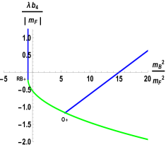
(a) $|\lambda|=0.25$

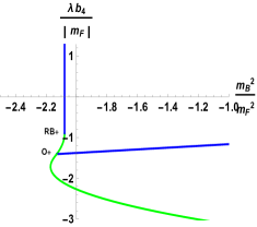
(b) $|\lambda|=0.43$

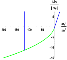
(c) $|\lambda|=0.75$

Figure 27: Numerically determined first order transition lines with $m_{F}\text{sgn}(\lambda)=1$ for different values of $|\lambda|$.

In each plot, the blue lines are second order transition lines while the green lines are the numerically determined first order transition lines. See equations (4.2), (4.2) in Section 4 for the equations describing the second order transition lines.

We should also mention that we can also analytically determine the first order line segment separating the $(+,+)$ and the $(+,-)$ phases. For $|\lambda|=0.25$, the analytic expression of this segment is given by,

$$\frac{m_{B}^{2}}{m_{F}^{2}}=\frac{9}{80}\left(26+9\sqrt{15}\right)\Big{(}\frac{\lambda\ b_{4}}{|m_{F}|}\Big{)}^{2}+\frac{7}{160}\left(26+9\sqrt{15}\right)\frac{\lambda\ b_{4}}{|m_{F}|}+\frac{7\left(7\sqrt{15}-122\right)}{1280}\ .$$ (188)

We have checked that our numerical solution perfectly matches with the analytically expression above.

We can also obtain an analytic expression for the first order line in the case of the $m_{F}=0$ section of the three dimensional parameter space, analysed in Section 4.1. The equation for the first order line is given by

$$m_{B}^{2}=\nu(\lambda)\ (\lambda b_{4})^{2}\ ,$$ (189)

where $\nu(\lambda)$ is a numerically determined function of $|\lambda|$. We plot the profile of $\nu(\lambda)$ vs. $|\lambda|$ in Figure 28.

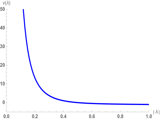
Figure 28: $\nu(\lambda)$ as a function of $|\lambda|$. The function $\nu(\lambda)$ appears in the equation for the first order line (189) in the $m_{F}=0$ section of the $\mathcal{N}=2$ phase diagram.

In the case of the first order lines in the northern and southern hemisphere sections $m_{F}=\pm|\mu|\text{sgn}(\lambda)$, the behaviour for large $m_{B}^{2}$ and $\lambda b_{4}$ is very well approximated by (189) since keeping $m_{F}$ fixed and taking $m_{B}^{2}$ and $\lambda b_{4}$ to $\infty$ is equivalent via the scalings (54) to keeping $m_{B}^{2}$ and $\lambda b_{4}$ fixed and taking $m_{F}$ to zero.

Appendix D Scaling limits

In this section we study scaling limits of the theory (1) in which the physics - or more precisely the dynamics about a particular saddle point of the theory (1) - simplifies. We will find scaling limits in which the dynamics of the corresponding saddle points of our theory reduces, in turn, to the critical fermion (CF) theory, the regular fermion (RF) theory, the regular boson (RB) theory, the critical boson (CB) theory. We also describe a scaling limit in which the resultant theory is a CFT describing the interaction of an RF plus CB theory.

The scaling limits we study in this section are all (generalisations of) scaling limits that have already been studied in Jain:2013gza (in the case of the RF, CB and mixed limits) and Aharony:2018pjn (in the case of the RB and CF limits). Our discussion in this section generalises the discussions of Jain:2013gza and Aharony:2018pjn in the following directions. First the discussions in the earlier literature focused exclusively on scaling limits in the $(+,+)$ and $(-,+)$ phases (i.e. the unHiggsed phase of the boson with either phase for the fermion). The new results for the Higgsed phase of the boson reported earlier in this paper allow us to study also the $(+,-)$ and $(-,-)$ phases and thereby discover new scaling limits. Second, the discussions in the earlier literature were always ‘local’ in the following sense: while the authors of Jain:2013gza and Aharony:2018pjn established that the dynamics of particular saddle points of the theory (1) reduces to the dynamics of simpler theories, the authors of those works were agnostic about whether the saddle point being studied is in fact the dominant saddle point of the theory under consideration. It is certainly possible (and we will see below that it happens many times) for the dynamics of a particular saddle point to simplify dramatically in a particular scaling limit, without implying anything significant for the physical behaviour of the full theory in the same scaling limit. This happens simply because the saddle point under consideration is subdominant in the scaling limit. In the current section we will shed light on this issue by studying the quantum effective potential (defined and computed earlier in this paper) in the scaling limits mentioned above. As the quantum effective potential has ‘global’ information of all phases of the theory, it allows us to definitively determine when (and whether) the ‘simplified’ scaled saddle points that we study below actually dominate the physical dynamics of our system.

Taking our lead from Jain:2013gza and Aharony:2018pjn , we first study scaling limits in which one of $c_{B}$ or $c_{F}$ is scaled to $\infty$ with the other fixed. This is conveniently done by setting

$$m_{F}=\mu\ ,\quad m_{B}^{2}=a_{1}\mu^{2}+a_{2}\mu+a_{3}\ ,\quad b_{4}=g_{1}\mu+g_{2}\ ,$$ (190)

and taking the limit $|\mu|\to\infty$ with both the dimensionless parameters ($a_{1}$ and $g_{1}$) and the dimensionful parameters ($a_{2}$, $a_{3}$ and $g_{2}$) held fixed.

Of course, only dimensionless ratios of dimensionful parameters are truly physical. The parametrization (190) is thus more invariantly stated in terms of ratios as

$$\frac{m_{B}^{2}}{m_{F}^{2}}=a_{1}+\frac{a_{2}}{\mu}+\frac{a_{3}}{\mu^{2}}\ ,\quad\frac{b_{4}}{m_{F}}=g_{1}+\frac{g_{2}}{\mu}\ ,$$ (191)

The parametrization (191) (or (190)) is extremely redundant: we have chosen to parametrize the two physical dimensionless ratios using two dimensionless parameters ($a_{1}$ and $g_{1}$) together with 3 dimensionful parameters ($a_{2}$, $a_{3}$ and $g_{2}$) and one additional auxiliary scale $\mu$. This highly redundant parametrization is useful under some circumstances as we now describe.

Quasi-bosonic scaling limits: As we will see below, there are special points in the space of ratios $(\frac{m_{B}^{2}}{m_{F}^{2}},\frac{b_{4}}{m_{F}})$ corresponding to the discrete values

$$\frac{m_{B}^{2}}{m_{F}^{2}}=\alpha_{i}\ ,\quad\frac{b_{4}}{m_{F}}=\gamma_{i}\ ,$$

where the discrete parameter $i$ labels the various special points at which our theory behaves in a very special way (see the CF and RB scaling limits below for the values of $\alpha_{i}$ and $\gamma_{i}$). It is also interesting to study our theory in the neighbourhood of these special points corresponding to deforming the values of $\frac{m_{B}^{2}}{m_{F}^{2}}$ and $\frac{b_{4}}{m_{F}}$ away from their special values. For this purpose we use the parametrization (191) together with the following natural convention:

$$a_{1}=\alpha_{i}\ ,\quad g_{1}=\gamma_{i}\quad\text{throughout the procedure of taking the scaling limit.}$$

With these conventions, we are now effectively using three dimensionful quantities and one auxiliary scale $\mu$ (so a total of three dimensionless ratios) to parametrize the two physically important dimensionless ratios. Clearly our parametrization still has a one parameter redundancy; the superfluity is simply the fact that the redefinitions

$$a_{2}=a_{2}^{\prime}+\frac{\xi}{\mu}\ ,\quad a_{3}^{\prime}=a_{3}-{\xi}\ ,$$ (192)

leave the ratios (191) unchanged and so define the same theory. In order to obtain a unique parametrization of our ratio space, we need a further convention to fix the ambiguity (192). We address this in each of the individual subsections below.

Quasi-fermionic scaling limits: We will also use the parametrization (191) to study the neighbourhood of special lines (rather than special points) in the space of ratios (191) (see the CB and RF limits described below). In this situation we simply choose the parameters $a_{1}$ and $g_{1}$ to lie on the special lines. In addition to the ambiguity (192), there is now a new potential ambiguity in this context. This is associated with motion along the special line – that is changing $a_{1}$ and $g_{1}$ such that they still lie on the special line and reabsorbing the changes in appropriate redefinitions of $a_{2}$, $a_{3}$ and $g_{2}$. We need an additional convention to fix this ambiguity.

To end the introductory part of this section we present the formulae for the fermionic and bosonic gaps in the $(\varepsilon,\pm)$ phases for convenient reference:

$$c_{F}=\frac{|{\tilde{m}}_{F}|}{1-\varepsilon|\lambda|}\quad\text{with}\quad{\tilde{m}}_{F}=m_{F}+2x_{4}\lambda\sigma\ ,\qquad c_{B}=\frac{2-2|\lambda|\pm 2}{-(2-|\lambda|)}\sigma\ ,$$ (193)

where $\sigma$ is determined by extremizing the quantum effective potential.

D.1 Fermionic scaling limits

In order to scale $c_{B}$ to $\infty$ with $c_{F}$ fixed, we need to scale $\sigma$ to $\infty$ such that the combination ${\tilde{m}}_{F}$ is fixed. We thus perform the following field redefinition from $\sigma$ to $\zeta$:

$$\sigma=-\frac{m_{F}}{2x_{4}\lambda}-\frac{\zeta}{2x_{4}\lambda}\ ,$$ (194)

with $\zeta$ held fixed in the limit $\mu\to\infty$. In the scaling limits under study, in other words, we are focusing our attention on the part of the $\sigma$ axis that lies around the ‘phase boundary’ at $\sigma=-\frac{m_{F}}{2x_{4}\lambda}$ in Figure 3.

Note: Our variable $\zeta$ is related to the variable $\zeta_{F}$ (defined in Appendix A) that usually appears in discussions of the critical fermion theory as

$$\zeta=\frac{4\pi\zeta_{F}}{\kappa_{F}}\ .$$ (195)

In the main text of this paper we will continue to use the variable $\zeta$ instead of $\zeta_{F}$ to avoid cluttering of notation.

When $x_{4}\lambda m_{F}>0$, the fermionic scaling limit focuses on the transition between $(-,+)$ and $(+,+)$ phases in Figure 3 and loses all information about the third phase in Figures 3(a) and 3(d) (since $m_{F}\to\infty$ with $x_{4}$ and $\lambda$ fixed). Note that when $x_{4}\lambda m_{F}>0$ the scaling limit lies entirely in the unHiggsed phase of the boson.

Similarly, when $x_{4}\lambda m_{F}<0$ the fermionic scaling limit focuses on the transition between the $(-,-)$ and $(+,-)$ phases and loses all information about the third phase in Figures 3(b) and 3(c). It follows that when $x_{4}\lambda m_{F}<0$, the scaling limit lies entirely in Higgsed phase of the boson.

Plugging (194) into the effective potential $U^{(\varepsilon,\pm)}$ (42), we get

$$\frac{2\pi}{N}U^{(\varepsilon,\pm)}(\zeta) =-\left(\psi_{\varepsilon}+\frac{x_{6}-\phi_{\pm}}{x_{4}^{3}}\right)\frac{\zeta^{3}}{8\lambda}-\left(-\frac{b_{4}}{2x_{4}^{2}\lambda}+\frac{3m_{F}}{8x_{4}^{3}\lambda}(x_{6}-\phi_{\pm})\right)\zeta^{2}$$

$$+\left(\frac{b_{4}m_{F}}{x_{4}^{2}\lambda}-\frac{m_{B}^{2}}{2x_{4}\lambda}-\frac{3m_{F}^{2}}{8x_{4}^{3}\lambda}(x_{6}-\phi_{\pm})\right)\zeta\ ,$$ (196)

where we have ignored the terms independent of $\zeta$. We also plug in the parametrization (190) in the above formula to get

$$\frac{2\pi}{N}U^{(\varepsilon,\pm)}(\zeta) =-\left(\psi_{\varepsilon}+\frac{x_{6}-\phi_{\pm}}{x_{4}^{3}}\right)\frac{\zeta^{3}}{8\lambda}+\left(\frac{\mu}{2x_{4}^{2}\lambda}\left(g_{1}-\tfrac{3}{4x_{4}}(x_{6}-\phi_{\pm})\right)+\frac{g_{2}}{2x_{4}^{2}\lambda}\right)\zeta^{2}$$

$$+\left(\frac{\mu^{2}}{2x_{4}^{2}\lambda}\left(2g_{1}-x_{4}a_{1}-\tfrac{3}{4x_{4}}(x_{6}-\phi_{\pm})\right)+\frac{\mu}{2x_{4}^{2}\lambda}(2g_{2}-x_{4}a_{2})-\frac{a_{3}}{2x_{4}\lambda}\right)\zeta\ ,$$ (197)

In order for the assumptions of this subsection to be self-consistent, the extremum value of $\zeta$, obtained by extremizing (D.1) w.r.t $\zeta$, should be of order unity (as we have assumed in (194)) rather than of order $\mu$. This requirement puts some constraints on the parameters $a_{1}$, $a_{2}$, $a_{3}$, $g_{1}$ and $g_{2}$ described above; solutions to this constraint generically yield the RF limit. If we also demand that not just the value of $\zeta$ at its extremum but that its whole quantum effective potential has a good $\mu\to\infty$ limit, we get additional constraints and land on the CF scaling limit. We take these up in turn, starting with the CF scaling limit.

D.1.1 The critical fermion limit

We wish to find a scaling limit in which the potential for the field $\zeta$ is finite, i.e. a limit in which the field $\zeta$ can fluctuate with a finite cost (as opposed to an infinite cost, which would be the case in an infinitely steep potential) in potential. As noted above, when $x_{4}\lambda m_{F}>0$, our scaling limit lies in the bosonic unHiggsed ($+$) phase; in this case the CF limit has previously been studied in Aharony:2018pjn . We will call this the ${\rm CF}+$ limit. On the other hand when $x_{4}\lambda m_{F}<0$ the CF scaling limit lies in the Higgsed ($-$) phase of the boson; this limit has not been studied before in the previous literature (because it involves working in the bosonic Higgsed phase). We will call this the ${\rm CF}-$ limit.

Note that while the coefficient of $\zeta^{3}$ in (D.1) is independent of $\mu$, the coefficients of $\zeta^{2}$ and $\zeta$ have terms proportional to $\mu$ and $\mu^{2}$. On physical grounds we would like this potential to be independent of $\mu$. One way to ensure this is to set the coefficient of every $\mu$-dependent term in the potential separately to zero. This gives the following constraints on the parameters in (190):

$$g_{1}=\gamma^{F}_{\pm}\ ,\quad a_{1}=\alpha^{F}_{\pm}\ ,\quad a_{2}=\frac{2g_{2}}{x_{4}}\ .$$ (198)

where the special values $\gamma^{F}_{\pm}$ and $\alpha^{F}_{\pm}$ correspond to the ${\rm CF}+$ and ${\rm CF}-$ limits and are given by

$$\gamma^{F}_{\pm}=\frac{3(x_{6}-\phi_{\pm})}{4x_{4}}\ ,\quad\alpha^{F}_{\pm}=\frac{3(x_{6}-\phi_{\pm})}{4x_{4}^{2}}\ .$$ (199)

(Here, of course, $x_{6}$ and $x_{4}$ refer to the dimensionless coupling constants of the original UV theory (2)). In these two scaling limits the effective potential reduces to the quantum effective potential for the CF theory

$$S_{\rm CF} =\int d^{3}x\bigg{[}i\varepsilon^{\mu\nu\rho}\frac{\kappa}{4\pi}\mathrm{Tr}(A_{\mu}\partial_{\nu}A_{\rho}-\frac{2i}{3}A_{\mu}A_{\nu}A_{\rho})+\bar{\psi}\gamma_{\mu}D^{\mu}\psi$$

$$\qquad\qquad\quad-\zeta(\bar{\psi}\psi-\frac{\kappa y_{2}^{2}}{4\pi})-\frac{\kappa y_{4}}{4\pi}\zeta^{2}+\frac{\kappa}{16\pi}x_{6}^{F}\zeta^{3}\bigg{]}\ ,$$ (200)

whose effective potential is given by (see Appendix A)

$$U_{\rm CF}(\zeta)=\left\{\begin{array}[]{ll}\displaystyle\frac{N}{2\pi}\left[(x_{6}^{F}-\psi_{+})\frac{\zeta^{3}}{8\lambda}-\frac{y_{4}}{2\lambda}\zeta^{2}+\frac{y_{2}^{2}}{2\lambda}\zeta\right]\ ,&\text{sgn}(\zeta)\text{sgn}(\lambda)<0\\ \displaystyle\frac{N}{2\pi}\left[(x_{6}^{F}-\psi_{-})\frac{\zeta^{3}}{8\lambda}-\frac{y_{4}}{2\lambda}\zeta^{2}+\frac{y_{2}^{2}}{2\lambda}\zeta\right]\ ,&\text{sgn}(\zeta)\text{sgn}(\lambda)>0\ .\end{array}\right.$$ (201)

where $\psi_{\varepsilon}$ was defined in (43).

The parameters $x_{6}^{F}$, $y_{2}$ and $y_{4}$ are given in terms of $g_{2}$, $a_{3}$ by

$$x_{6}^{F}=x_{6}^{F\pm}=-\frac{x_{6}-\phi_{\pm}}{x_{4}^{3}}\ ,\quad y_{4}=-\frac{g_{2}}{x_{4}^{2}}\ ,\quad y_{2}^{2}=-\frac{a_{3}}{x_{4}}\ .$$ (202)

From (194), it is apparent that we reach the ${\rm CF}\pm$ limit when $\text{sgn}(m_{F}/x_{4}\lambda)=\pm 1$.

The effective potential (201) is bounded from below if and only if $x_{6}^{F}$ lies in the interval $(\psi_{-},\psi_{+})$. When this is not the case, (201) unbounded from below, and one of the following things must be true of the UV theory:

1. Either the potential of the UV theory is also unbounded from below,

2. Else the UV potential has a minimum that lies outside the scaling limit with a lower free energy than any configuration that can be accessed within the scaling limit. In this case the dominant saddle point of UV theory is not captured by our scaling limit.

In either of the two cases above the scaling limit is not really interesting (in the first case because the UV theory itself is unstable, and in the second case because the scaling limit focuses on a subdominant saddle point).

If, on the other hand, $x_{6}^{F}$ does lie in the interval $(\psi_{-},\psi_{+})$ it is at least possible that the scaling limit focuses on a region of $\sigma$ that includes the dominant saddle point of a well-defined UV theory. Whether that is actually the case or not requires a more detailed study of saddle points outside the scaling limit; we will perform such an analysis in the special case of the ${\cal N}=2$ theory below.

We now address the ambiguities in our description referred to around equation (191). In our scaling ansatz, the ultraviolet theory is parametrized by two dimensionless parameters ($a_{1}$ and $g_{1}$), three dimensionful parameters ($a_{2}$, $a_{3}$ and $g_{2}$) and one mass scale $\mu$. In our computation above, we have chosen the convention that each $\mu$-dependent term in the potential is set to zero separately. This ensures that the dimensionless parameters $a_{1}$ and $g_{1}$ are fixed to their limiting values (cf. (198)) even when $\mu$ is finite but large. Similarly, of the three dimensionful parameters, two are related to each other by the last equality $2g_{2}=x_{4}a_{2}$ in (198), again even when $\mu$ is finite but large. Thus, at the end of the scaling limit (where we have lost the mass scale $\mu$), we have two dimensionful parameters (conveniently chosen to be $g_{2}$ and $a_{3}$, cf. (202)) which matches the physics of the critical fermion theory deformed by its two relevant parameters.

In the just-concluded computation, we adopted the convention that each $\mu$-dependent term is set to zero separately. However, we emphasize that this is a choice that fixes the ambiguity of parametrization (discussed around (190)) and not a physical requirement as we now pause to explain.

Let us focus on the coefficient of $\zeta$ in (D.1) (the discussion for the coefficient of $\zeta^{2}$ proceeds analogously). If we denote the coefficient of $\zeta$ by $A\mu^{2}+B\mu+C$ it is not strictly really necessary to set $A$ and $B$ separately to zero. Instead, we could set $A=\frac{p_{1}}{\mu}+\frac{p_{2}}{\mu^{2}}$ and $B=-p_{1}+\frac{q_{2}}{\mu}$ so that the $\mu$-dependent pieces vanish. In order to maintain the $\mu$-independent part at its previous value, we need to redefine it by $C^{\prime}=C-p_{2}-q_{2}$. In terms of the parametrization (191), this corresponds to the redefinition

$$2g_{1}^{\prime}-x_{4}a_{1}^{\prime}=2g_{1}-x_{4}a_{1}+\frac{p_{1}}{\mu}+\frac{p_{2}}{\mu^{2}}\ ,$$

$$2g_{2}^{\prime}-x_{4}a_{2}^{\prime}=2g_{2}-x_{4}a_{2}-p_{1}+\frac{q_{2}}{\mu}\ ,$$

$$-x_{4}a_{3}^{\prime}=-x_{4}a_{3}-p_{2}-q_{2}\ .$$ (203)

Suppose we first fix the convention alluded to in the discussion around (191) that $a_{1}$ and $g_{1}$ are fixed to the special values $\alpha^{F}_{\pm}$ and $\gamma^{F}_{\pm}$ (this is ensured in our choice of setting each $\mu$-dependent term to zero separately). This kills the arbitrary constants $p_{1}$ and $p_{2}$ in (D.1.1). The remaining ambiguity resides in the constant $q_{2}$ and is the ambiguity referred to (192). This ambiguity is also killed by our choice of setting each $\mu$-dependent term to zero separately.

D.1.2 The regular fermion limit

In the previous subsection we studied a scaling limit (or RG flow) under which the theory (2) reduces to the CF theory. As we have reviewed in Appendix A, the quantum effective action for the CF theory is nontrivial (i.e. allows for a fluctuating $\zeta$ field). This is the reason we determined our scaling limit in the last subsection by demanding that the quantum effective action for $\zeta$ is nontrivial.

In this subsection we search for a scaling limit in which our theory reduces instead to the (less special) RF theory. As we review in Appendix A, the quantum effective action for the RF is trivial - or more precisely infinitely deep around an extremum which, however, occurs at a finite value of $\zeta$. For this reason in this section we search for a scaling limit in which the effective potential takes the appropriate form; i.e. is infinitely deep at a finite value of $\zeta$.

One way of achieving this goal is simply to set the coefficient of $\mu^{2}$ in coefficient of $\zeta$ in the quantum effective potential (D.1) to zero. This gives

$$2g_{1}=x_{4}a_{1}+\frac{3}{4x_{4}}(x_{6}-\phi_{\pm})\ ,$$ (204)

which can be rewritten as

$$2\left(g_{1}-\gamma_{\pm}^{F}\right)=x_{4}\left(a_{1}-\alpha_{\pm}^{F}\right)\ .$$ (205)

where $\gamma_{\pm}^{F}$ and $\alpha_{\pm}^{F}$, defined in (199), are the values of $g_{1}$ and $a_{1}$ at which we obtain the CF theory. The potential in (D.1) becomes

$$\frac{2\pi}{N}U(\zeta) =-\left(\psi_{\varepsilon}+\frac{x_{6}-\phi_{\pm}}{x_{4}^{3}}\right)\frac{\zeta^{3}}{8\lambda}+\frac{\zeta^{2}}{2x_{4}^{2}\lambda}\left(\mu(g_{1}-\gamma^{F}_{\pm})+g_{2}\right)$$

$$+\frac{\zeta}{2x_{4}^{2}\lambda}\left(\mu(2g_{2}-x_{4}a_{2})-x_{4}a_{3}\right)\ ,$$ (206)

The terms in the potential (D.1.2) that are proportional to $\mu$ can be rewritten by completing squares as

$$\frac{\mu(g_{1}-\gamma^{F}_{\pm})}{2x_{4}^{2}\lambda}\left(\left(\zeta+\frac{(2g_{2}-x_{4}a_{2})}{2(g_{1}-\gamma^{F}_{\pm})}\right)^{2}-\frac{(2g_{2}-x_{4}a_{2})^{2}}{4(g_{1}-\gamma^{F}_{\pm})^{2}}\right)\ .$$ (207)

In the $\mu\to\infty$ limit, the potential is dominated by the above term. Suppose the prefactor $\frac{\mu(g_{1}-g^{F}_{1\pm})}{2x_{4}^{2}\lambda}$ is positive:

$$\frac{\mu(g_{1}-\gamma^{F}_{\pm})}{2x_{4}^{2}\lambda}\geq 0\ ,\quad{\rm i.e.}\quad{\text{sgn}}(g_{1}-\gamma^{F}_{\pm})={\text{sgn}}(\lambda\mu)\ .$$ (208)

In this case the following value of $\zeta$ is a minimum of the above term and the variable $\zeta$ freezes to this value in the $\mu\to\infty$ limit:

$$\zeta=-\frac{2g_{2}-x_{4}a_{2}}{2(g_{1}-\gamma^{F}_{\pm})}+{\cal O}(1/\mu)\ ,$$ (209)

where we have indicated possible $1/\mu$ corrections to the extremum which vanish in the $\mu\to\infty$ limit. In this section, we adopt the convention that the ${\cal O}(1/\mu)$ correction to (209) vanishes so that $\zeta$ takes the following precise value at the minimum of the potential:

$$\zeta_{\rm min.}=-\frac{2g_{2}-x_{4}a_{2}}{2(g_{1}-\gamma^{F}_{\pm})}\ .$$ (210)

It is natural to label the above minimum of $\zeta$ as

$$m_{F}^{\rm reg}=-\zeta_{\rm min.}=\frac{2g_{2}-x_{4}a_{2}}{2(g_{1}-\gamma^{F}_{\pm})}\ ,$$ (211)

since this minimum value of $\zeta$ will serve as the mass parameter of the regular fermion theory.

The requirement that we have already enunciated - that the ${\cal O}(1/\mu)$ correction to (209) vanish - holds only if the special value of $\zeta$ described in (210) also separately extremize the $\mu$-independent part of the potential listed in (D.1.2). This occurs provided that

$$\left(\psi_{\varepsilon}+\frac{x_{6}-\phi_{\pm}}{x_{4}^{3}}\right)\frac{3(m_{F}^{\rm reg})^{2}}{8\lambda}+\frac{g_{2}m_{F}^{\rm reg}}{x_{4}^{2}\lambda}+\frac{a_{3}}{2x_{4}\lambda}=0\ .$$ (212)

The solution (209) is a local minimum - rather than a local maximum - of the potential $U(\zeta)$ in (D.1.2) provided that (208) holds. Note that the LHS of (208) changes sign as $g_{1}$ crosses $\gamma^{F}_{\pm}$, i.e. passes the critical fermion scaling limit. It follows that the regular fermion fixed line is locally stable only on one side of the CF scaling limit, as expected on general grounds.

(205) and (212) and (211) are three conditions on the 5 parameters that appear in (191). In more detail (205) gives one relation between the two dimensionless parameters $a_{1}$ and $g_{1}$ in (191) while (212) and (211) gives two relationships between the three dimensionful parameters $g_{2}$, $a_{2}$ and $a_{3}$ and the one physical dimensionful parameter of the IR theory, namely $m_{F}^{\rm reg}$. Even with all the conventions adopted in this subsection, in other words, we still have landed on a two parameter set of scaling limits rather than a unique scaling limit as in the previous subsection. The reason for this, of course, is that the RF limit occurs on a line in the phase diagram of our theory- rather than on a point in the phase diagram of our theory as was the case in the previous section. The shift in dimensionless parameters that was unfixed by (205) simply moves us along the line of RF theories in our phase diagram. And the one unfixed massive parameter also actually does the same. To see the last point note that that $m_{F}^{\rm reg}$ depends only on the combination $2g_{2}-x_{4}a_{2}$. Consequently, the unfixed massive parameter is parametrized by the simultaneous shift

$$2g_{2}=2g^{\prime}_{2}-p\ ,\quad x_{4}a_{2}=x_{4}a^{\prime}_{2}-p\ ,$$ (213)

that leaves $m_{F}^{\rm reg}$ invariant. A glance at (191) will convince the reader that this shift also moves us along the line of RF theories.

As both the moves above, i.e. shifts in $a_{1}$ and $g_{1}$ that continue to obey (205) and the shifts in $a_{2}$, $g_{2}$ in (213) move us along the same line in phase space, there is a linear combination of these shifts that do not move us in phase space; this linear combination is an unfixed ambiguity of our parametrization of this scaling limit. This ambiguity is given by (213) together with

$$2g_{1}=2g^{\prime}_{1}+\frac{p}{\mu}\ ,\quad x_{4}a_{1}=x_{4}a^{\prime}_{1}+\frac{p}{\mu}\ .$$ (214)

(as a check one can verify that above two shifts (213), (214) leave the potential in (D.1.2) unchanged).

In order to reach the scaling limit of this section, on physical grounds we needed only to impose a single condition, namely that (205) hold upto corrections of order $1/\mu$. The extra conditions we have imposed, namely that this equation hold exactly rather than upto corrections of order $1/\mu$ and also that the terms order $1/\mu$ in (209) vanish - were imposed for convenience rather than necessity, and served to fix some of the ambiguities of our parametrization (discussed under (191)) in a manner similar to the discussion of the previous subsection.

D.2 Bosonic scaling limits

By definition, a bosonic scaling limit is one in which the bosonic pole mass $c_{B}$ stays finite while $c_{F}$ is scaled to $\infty$ so that the resultant theory is purely bosonic. From the second of (193) we see that $c_{B}$ is proportional to $\sigma$, which implies that $\sigma$ must stay finite in the scaling limit $\mu\to\infty$. As a consequence the effective potential in the bosonic scaling limit is a function of $\sigma$ (rather than of $\zeta$ as in the fermionic limit), and the bosonic analogue of (D.1) is obtained by plugging the definition of ${\tilde{m}}_{F}=m_{F}+2\lambda x_{4}\sigma$ in terms of $\sigma$ into the original expression for the Landau-Ginzburg potential (42). We find

$$U^{(\varepsilon,\pm)}(\sigma)=\frac{N}{2\pi}\Big{[}\left(x_{6}-\phi_{\pm}+x_{4}^{3}\psi_{\varepsilon}\right)\lambda^{2}{\sigma}^{3}+\left({b}_{4}+\tfrac{3}{4}x_{4}^{2}\psi_{\varepsilon}m_{F}\right)2\lambda{\sigma}^{2}\\ +\left({m}_{B}^{2}+\tfrac{3}{4}x_{4}\psi_{\varepsilon}m_{F}^{2}\right){\sigma}\Big{]}\ ,$$ (215)

where we have ignored a constant term proportional to $\mu^{3}$. Plugging in the scalings in (190), the above expression becomes

$$U^{(\varepsilon,\pm)}(\sigma)=\frac{N}{2\pi}\Big{[}\left(x_{6}-\phi_{\pm}+x_{4}^{3}\psi_{\varepsilon}\right)\lambda^{2}{\sigma}^{3}+\left(\mu(g_{1}+\tfrac{3}{4}x_{4}^{2}\psi_{\varepsilon})+g_{2}\right)2\lambda{\sigma}^{2}\\ +\left(\mu^{2}(a_{1}+\tfrac{3}{4}x_{4}\psi_{\varepsilon})+a_{2}\mu+a_{3}\right){\sigma}\Big{]}\ ,$$ (216)

D.2.1 Regular boson limit

As in the CF limit, we obtain the regular boson limit by substituting in the scalings (190) into (216). The coefficient of $\sigma$ in (216) has a term proportional to $\mu^{2}$ and a term proportional to $\mu$ (in addition to the constant piece), while the coefficient of $\sigma^{2}$ has a term proportional to $\mu$ (in addition to a constant). As in Section D.1.1 we tune to the RB limit by setting all three coefficients mentioned above to zero. This requirement gives

$$g_{1}=\gamma^{B}_{\pm}\ ,\quad a_{1}=\alpha^{B}_{\pm}\ ,\quad a_{2}=0\ ,$$ (217)

where $\gamma_{\pm}^{B}$ and $\alpha_{\pm}^{B}$ are given by

$$\gamma^{B}_{\pm}=-\frac{3x_{4}^{2}}{4}\psi_{\pm}\ ,\quad\alpha^{B}_{\pm}=-\frac{3x_{4}}{4}\psi_{\pm}\ ,$$ (218)

where $\psi_{\pm}$ was defined in (43). The effective potential (216) reduces to that of the regular boson:

$$U_{\rm RB}(\sigma)=\left\{\begin{array}[]{lr}\frac{N}{2\pi}\left[(x_{6}^{B}-\phi_{+})\lambda^{2}\sigma^{3}+2{\tilde{b}}_{4}\lambda\sigma^{2}+{\tilde{m}}_{B}^{2}\sigma\right]&\sigma<0\ ,\\ \frac{N}{2\pi}\left[(x_{6}^{B}-\phi_{-})\lambda^{2}\sigma^{3}+2{\tilde{b}}_{4}\lambda\sigma^{2}+{\tilde{m}}_{B}^{2}\sigma\right]&\sigma>0\ ,\end{array}\right.$$ (219)

with

$$x_{6}^{B}=x_{6}^{B\pm}=x_{6}+x_{4}^{3}\psi_{\pm}\ ,\quad{\tilde{b}}_{4}=g_{2}\ ,\quad{\tilde{m}}_{B}^{2}=a_{3}\ .$$ (220)

where the sign $\pm$ applies when the infinitely massive fermion which is being integrated out is in its $+$ or the $-$ phase respectively. In the scaling limit where we keep $\sigma$ to be $\mathcal{O}(1)$, we see that $\text{sgn}({\tilde{m}}_{F})=\text{sgn}(m_{F})$; it follows that the fermion is in the $\pm$ phase when $\text{sgn}(m_{F})\text{sgn}(\lambda)=\pm 1$ respectively. We refer to these two cases as the ${\rm RB\pm}$ scaling limits respectively.

As the RB limit focuses on finite values of $\sigma$, it zeroes in on the phases around $\sigma=0$ in each of the four cases listed in Fig 3. In particular when $\lambda m_{F}>0$ our limit (the ${\rm RB}+$ limit) focuses on the ‘transition region’ between the $(+,+)$ and $(+,-)$ phases (discarding the $(-,+)$ phase in the case the $x_{4}>0$ and discarding the $(-,-)$ phase in the case that $x_{4}<0$). On the other hand in the case that $\lambda m_{F}<0$ our limit focuses on the ‘transition between’ $(-,+)$ and $(-,-)$ (discarding the $(+,-)$ phase when $x_{4}>0$ and discarding the $(-,-)$ phase when $x_{4}<0$.

When $x_{6}^{B}$ lies outside the interval $(\phi_{-},\phi_{+})$, the effective potential (219) is unbounded from below (as described in Appendix A). When this happens (as in Section D.1.1) the saddle point we are focusing on in this subsubsection cannot represent the global minimum of the UV effective potential. In this situation, as in Section D.1.1, the UV potential is either unbounded from below or has another saddle point (other than the one focused on in this subsubsection) which represents the dominant phase of the theory. When, on the other hand, $x_{6}^{B}$ lies in the $(\phi_{-},\phi_{+})$, the saddle point focused on in this subsubsection may (or may not) represent the global minimum of the UV effective potential depending on details.

D.2.2 The critical boson scaling limit

The discussion here is very similar to the regular fermion scaling limit. In order to go close to the critical boson fixed point, one needs to have a competition between the $\sigma^{2}$ and $\sigma$ deformations. This allows at most a linear dependence on the mass scale $\mu$ in the effective potential (216). One way to achieve this - the way we adopt in this paper - is to set the coefficient of $\mu^{2}$ to zero .

Demanding that the term proportional to $\mu^{2}$ in the coefficient of $\sigma$ is zero gives

$$a_{1}=-\frac{3}{4}x_{4}\psi_{\pm}\ ,$$ (221)

or

$$a_{1}-\alpha_{\pm}^{B}=0\ ,$$ (222)

and the effective potential (216) becomes

$$\frac{2\pi}{N}U^{(\varepsilon,\pm)}(\sigma) =\left(x_{6}-\phi_{\pm}+x_{4}^{3}\psi_{\varepsilon}\right)\lambda^{2}{\sigma}^{3}+\left(\left(g_{1}+\tfrac{3}{4}x_{4}^{2}\psi_{\varepsilon}\right)\mu+g_{2}\right)2\lambda{\sigma}^{2}+\left(a_{2}\mu+a_{3}\right){\sigma}\ ,$$ (223)

up to a constant that scales as $\mu^{3}$. In the $\mu\to\infty$ limit, the part of the potential that is dominant is

$$\mu\left(2\lambda(g_{1}-\gamma^{B}_{\pm})\sigma^{2}+a_{2}\sigma\right)=2\lambda\mu(g_{1}-\gamma_{\pm}^{B})\left(\left(\sigma+\frac{a_{2}}{4\lambda(g_{1}-\gamma_{\pm}^{B})}\right)^{2}-\frac{a_{2}^{2}}{16\lambda^{2}(g_{1}-\gamma_{\pm}^{B})^{2}}\right)\ .$$ (224)

The above potential has an extremum at

$$\sigma=-\frac{a_{2}}{4\lambda(g_{1}-\gamma_{\pm}^{B})}\ ,$$ (225)

which is a local minimum provided that

$$2\lambda\mu(g_{1}-\gamma_{\pm}^{B})\geq 0.$$ (226)

When this is satisfied, $\sigma$ freezes at the extremum in the $\mu\to\infty$ limit:

$$\sigma\equiv-\tfrac{1}{2}m_{B}^{\rm cri}=-\frac{a_{2}}{4\lambda(g_{1}-g_{1\pm}^{B})}\ .$$ (227)

The minimum value of $\sigma$ also has to separately minimise the $\mu$-independent part of the potential, giving rise to the equation

$$a_{3}=2\lambda m_{B}^{\rm cri}g_{2}-\frac{3}{4}(x_{6}-\phi_{\pm}+\psi_{\varepsilon})(m_{B}^{\rm cri})^{2}\ .$$ (228)

When the converse of (226) is true, the extremum (227) is a local maximum rather than a minimum, and cannot represent the true phase of the UV theory. As in the case of the RF scaling limit, (222) is a line in parameter space that runs through the RB point (217). The condition (226) is obeyed on one side of the RB point and not the other. In the neighbourhood of the point (217), the condition (226) is obeyed along the part of the RB phase diagram that corresponds to the second order phase transition line that emanates out of the RB conformal point (see the phase diagrams listed in Figure 25 and also Figures 7,8,9 in Aharony:2018pjn and Figures 6,8,11 in Dey:2018ykx ).

D.3 The CB-RF scaling limit

D.3.1 Anticipating the scaling limit

We have explained above that the ${\rm RF}\pm$ limit occurs in the neighbourhood of the line

$$2\left(\frac{b_{4}}{m_{F}}-\gamma_{\pm}^{F}\right)=x_{4}\left(\frac{m_{B}^{2}}{m_{F}^{2}}-\alpha_{\pm}^{F}\right)\quad\text{with}\quad\frac{m_{F}}{\lambda}\left(\frac{b_{4}}{m_{F}}-\gamma_{\pm}^{F}\right)\geq 0\ .$$ (229)

where $\gamma^{F}_{\pm}$ and $\alpha^{F}_{\pm}$ were defined in (199). The $+$ sign in the equation above applies when $x_{4}\lambda m_{F}>0$, while the $-$ sign applies when $x_{4}\lambda m_{F}<0$. To remind the reader, the ${\rm RF}+$ limit corresponds to regular fermions coupled to $SU(N)_{k}$ Chern-Simons gauge fields while the ${\rm RF}-$ limit corresponds to regular fermions coupled to $SU(N-1)_{k}$ Chern-Simons gauge fields.

On the other hand the ${\rm CB}\pm$ limit occurs in the neighbourhood of the line

$$\frac{m_{B}^{2}}{m_{F}^{2}}-\alpha_{\pm}^{B}=0\quad\text{with}\quad\frac{m_{F}}{\lambda}\left(\frac{b_{4}}{m_{F}}-\gamma_{\pm}^{B}\right)\geq 0\ ,$$ (230)

where where $\gamma^{B}_{\pm}$ and $\alpha^{B}_{\pm}$ were defined in (218) and the $\pm$ sign applies when $\lambda m_{F}$ is correspondingly positive or negative. Again, the ${\rm CB}+$ limit corresponds to critical bosons coupled to $SU(N)_{k}$ Chern-Simons gauge fields whereas the ${\rm CB}-$ limit corresponds to critical bosons coupled to $SU(N)_{k-1}$ Chern-Simons gauge fields.

Let us, for a moment, view the equations (229) and (230) each as defining two dimensional manifolds in the three dimensional space parametrized by the three variables $b_{4}$, $m_{F}$ and $m_{B}^{2}$. For any given values of $x_{4}$ and $x_{6}$, all four half-paraboloids in (229) and (230) (two for $\lambda m_{F}>0$ and two for $\lambda m_{F}<0$) occur in the three dimensional relevant parameter space. It is easy to see that these four half-paraboloids have a common intersection at the following half-line in three-dimensional parameter space:

$$\lambda m_{F}=0\ ,\quad m_{B}^{2}=0\ ,\quad\lambda b_{4}\geq 0\ .$$ (231)

A point in the phase diagram of our theory is associated with an equivalence class of points in $(m_{F},b_{4},m_{B}^{2})$ space; points in the same equivalence classes are related by scalings which act as $(m_{F},b_{4},m_{B}^{2})\rightarrow(\Lambda m_{F},\Lambda b_{4},\Lambda^{2}m_{B}^{2})$ for any positive $\Lambda$. Clearly the points on the ray (231) all lie in the same equivalence class and so correspond to a single point in the phase diagram of the theory, which we call the CB-RF conformal point. The neighbourhood of this point corresponds to massive critical bosons and regular fermions and should also be obtained as an appropriate scaling limit of the theory (1).

D.3.2 The scaling limit

Thus, in order to study the CB-RF point, one has to keep both $c_{B}$ and $c_{F}$ finite in the scaling limit. The equations for $c_{B}$ and $c_{F}$ in (193) tell us that ${\tilde{m}}_{F}$ and $\sigma$ have to be kept fixed in the scaling limit, and consequently that $m_{F}$ has to be kept fixed. The scaling behaviour in (190) is not well-suited to this end; hence, we adopt a different scaling limit first discussed in Jain:2013gza : we take the limit $\mu\to\infty$ with

$$m_{B}^{2}=a_{1}\mu^{2}\ ,\quad b_{4}=g_{0}\mu^{2}+g_{1}\mu+g_{2}\ ,\quad m_{F}\ \text{fixed}\ .$$ (232)

Some features of the scaling (232) are easy to understand. Recall that the Landau Ginzburg potential four branches whose ranges of validity are given in (2.5). The transition between a Higgsed and unHiggsed phase occurs at $\sigma=0$ while transition between a $\pm$ fermionic phase occurs at $\sigma=-\frac{m_{F}}{2x_{4}\lambda}$. In the CB-RF limit, our IR theory is able to undergo both kinds of phase transition. This can only happen if $-\frac{m_{F}}{2x_{4}\lambda}$ stays fixed in the limit $\mu\to\infty$, explaining why $m_{F}$ is held fixed in the limit. In order to reproduce CB-RF physics, the quantum effective potential must also have a minimum at a value of $\sigma$ that is held fixed as $\mu\to\infty$; this requirement essentially fixes the relative scalings of $b_{4}$ and $m_{B}^{2}$, as we will see in more detail below.

Let us now look at the potential of the theory:

$$\frac{2\pi}{N}U^{(\varepsilon,\pm)}(\sigma) =\left(x_{6}-\phi_{\pm}+x_{4}^{3}\psi_{\varepsilon}\right)\lambda^{2}{\sigma}^{3}+\left({b}_{4}+\tfrac{3}{4}x_{4}^{2}m_{F}\psi_{\varepsilon}\right)2\lambda{\sigma}^{2}+\left({m}_{B}^{2}+\tfrac{3}{4}x_{4}m_{F}^{2}\psi_{\varepsilon}\right){\sigma}\ ,$$ (233)

where we have again dropped the constant term which scales as $\mu^{3}$. In the scaling limit, the terms proportional to $\mu^{2}$ dominate:

$$\mu^{2}(2\lambda g_{0}\sigma^{2}+a_{1}\sigma)=2\lambda\mu^{2}g_{0}\left(\left(\sigma+\frac{a_{1}}{4\lambda g_{0}}\right)^{2}-\frac{a_{1}^{2}}{16\lambda^{2}g_{0}^{2}}\right)\ .$$ (234)

Suppose the prefactor $\lambda g_{0}$ in the above expression is positive

$$\lambda g_{0}\geq 0\ .$$ (235)

Then the extremum of the potential (234) is a minimum and $\sigma$ freezes at the minimum given by

$$\sigma=-\frac{a_{1}}{4\lambda g_{0}}=\lim_{\mu\to\infty}-\frac{m_{B}^{2}}{4\lambda b_{4}}\ .$$ (236)

Note that this looks exactly like the scaling limit that produces the critical boson theory from the regular boson theory with critical boson mass parameter $m_{B}^{\rm cri}=\lim\frac{m_{B}^{2}}{2\lambda b_{4}}$. Thus, it is natural to call the extremum value of $\sigma$ in (236) as

$$\sigma=-\frac{a_{1}}{4\lambda g_{0}}\equiv-\tfrac{1}{2}m_{B}^{\rm cri}\ .$$ (237)

This also freezes the effective fermion mass parameter ${\tilde{m}}_{F}$ at the value

$${\tilde{m}}_{F}=m_{F}-\lambda x_{4}m_{B}^{\rm cri}\equiv m_{F}^{\rm reg}\ ,$$ (238)

which is exactly of the form of a mass for the regular fermion theory.

Moreover, as in previous subsections, we fix some of the ambiguities of our redundant parametrization of our scaling limit by demanding that (236) hold exactly rather than only upto correction terms of order $1/\mu^{2}$. This precisely determined value of $\sigma$ must extremize the quantum effective potential

$$3\left(x_{6}-\phi_{\pm}+x_{4}^{3}\psi_{\varepsilon}\right)\lambda^{2}{\sigma}^{2}+\left({b}_{4}+\tfrac{3}{4}x_{4}^{2}m_{F}\psi_{\varepsilon}\right)4\lambda{\sigma}+\left({m}_{B}^{2}+\tfrac{3}{4}x_{4}m_{F}^{2}\psi_{\varepsilon}\right)=0\ .$$ (239)

The terms proportional to $\mu^{2}$ already cancel by virtue of (236). The term proportional to $\mu$ is zero if and only if we set $g_{1}=0$; we make this choice. The $\mu$-independent term is zero if the following relation is satisfied:

$$-2\lambda g_{2}m_{B}^{\rm cri}+\tfrac{3}{4}(x_{6}-\phi_{\pm})\lambda^{2}(m_{B}^{\rm cri})^{2}+\tfrac{3}{4}x_{4}\psi_{\varepsilon}\left(-2\lambda m_{B}^{\rm cri}x_{4}m_{F}+m_{F}^{2}+x_{4}^{2}\lambda^{2}(m_{B}^{\rm cri})^{2}\right)=0\ .$$ (240)

That is

$$g_{2}=\frac{\tfrac{3}{4}\left(x_{6}-\phi_{\pm}\right)\lambda^{2}(m_{B}^{\rm cri})^{2}+\frac{3}{4}x_{4}\psi_{\varepsilon}(m_{F}^{\rm reg})^{2}}{2\lambda m_{B}^{\rm cri}}\ .$$ (241)

Thus, we seem to obtain a theory of gauged critical bosons and regular fermions with masses $m_{B}^{\rm cri}$ and $m_{F}^{\rm reg}$ with the ultraviolet parameters given in terms of these by

$$m_{B}^{2}=\text{sgn}(m_{B}^{2})\mu^{2}\ ,\quad m_{F}=m_{F}^{\rm reg}+x_{4}\lambda m_{B}^{\rm cri}\ ,\quad b_{4}=\frac{1}{2\lambda m_{B}^{\rm cri}}\mu^{2}+g_{2}\ ,$$ (242)

with the value of $g_{2}$ given in (241).

D.3.3 Matching with previous scaling limits

The condition (235) can be rewritten in terms of $b_{4}$ as

$$\lambda b_{4}\geq 0\quad\text{in the limit}\quad\mu\to\infty\ .$$ (243)

This is exactly the condition on $\lambda b_{4}$ that one has in the intersection of the RF and CB half-paraboloids in (231).

The conformal RF-CB point corresponds to the point where $c_{B}=c_{F}=0$, which occurs when $m_{B}^{\rm cri}=m_{F}^{\rm reg}=0$. In terms of the ultraviolet parameters this point is given by

$$m_{F}=0\ ,\quad m_{B}^{2}=0\ ,$$ (244)

where we have used (238) and the second equality of (236). The equations in (244) and the condition in (243) precisely describe the intersection of the ${\rm RF}\pm$ and ${\rm CB}\pm$ half-paraboloids in (231).

Suppose one turns on the mass parameter $m_{F}^{\rm reg}$ for the fermion while keeping the boson mass at zero. This is expected to further flow down to the critical boson conformal theories ${\rm CB}\pm$ where the sign $\pm$ corresponds to $\text{sgn}(\lambda m_{F}^{\rm reg})=\pm 1$. This sign coincides with the sign of $\lambda m_{F}$ when $m_{B}^{\rm cri}=0$ as is obvious from the formula (238). The condition $\text{sgn}(\lambda m_{F})=\pm 1$ for the occurrence of ${\rm CB}\pm$ limits is precisely the condition we obtained in the critical boson scaling limit (cf. Section D.2.2).

Similarly, if one turns on $m_{B}^{\rm cri}$ and keeps $m_{F}^{\rm reg}$ fixed at zero, the theory further flows down to the ${\rm RF}\pm$ theories, where the sign is given by the sign of $m_{B}^{\rm cri}$. The condition $m_{F}^{\rm reg}=0$ gives (from (238))

$$m_{F}=\lambda x_{4}m_{B}^{\rm cri}\ ,$$ (245)

which relates the sign of $m_{B}^{\rm cri}$ to the sign of $\lambda m_{F}x_{4}$ as $\text{sgn}(m_{B}^{\rm cri})=\text{sgn}(\lambda m_{F}x_{4})$. Thus, we get the ${\rm RF}\pm$ theories when $\text{sgn}(\lambda m_{F}x_{4})=\pm 1$ which is precisely the condition we obtained in the regular fermion scaling limit (cf. Section D.1.2).

The $m_{B}^{\rm cri}=0$ and $m_{F}^{\rm reg}=0$ loci correspond to

$$\text{Critical boson},\ m_{B}^{\rm cri}=0: \qquad\ \ m_{B}^{2} =0\ ,$$

$$\text{Regular fermion},\ m_{F}^{\rm reg}=0: \qquad\frac{\lambda m_{F}}{\lambda b_{4}} =\frac{\lambda^{2}x_{4}}{2}\frac{m_{B}^{2}}{(\lambda b_{4})^{2}}\ .$$ (246)

These are precisely the same equations that define the CB and RF conformal scaling limits in (230) and (229) in the neighbourhood of $m_{F}=0$, as can be easily seen from those equations. For a fixed large (positive) value of $\lambda b_{4}$ we plot these lines in $(m_{B}^{2},\lambda m_{F})$ space in Figure 29.

Figure 29: The features of the CB-RF theory in the neighbourhood of the CB-RF conformal point depicted as a thick dot at the origin. The blue lines correspond to the various quasi-fermionic conformal theories that emanate / terminate at the origin. The various topological phases are also shown. The figure is plotted for $x_{4}>0$.

Clearly, these lines coincide with the CB and RF lines in (229) and (230) at the same value of $\lambda b_{4}$. A generic deformation with masses for both the bosons and fermions would lead to the appropriate one of the four topological phases $(\pm,\pm)$. These are separated by the four transition lines.

The previous discussion further demonstrates that the regular fermion and the critical boson lines terminate at the CB-RF conformal point.

References

- (1) S. Jain, S. Minwalla, and S. Yokoyama, Chern Simons duality with a fundamental boson and fermion, JHEP 1311 (2013) 037, [arXiv:1305.7235].
- (2) G. Gur-Ari and R. Yacoby, Three Dimensional Bosonization From Supersymmetry, JHEP 11 (2015) 013, [arXiv:1507.04378].
- (3) O. Aharony, S. Jain, and S. Minwalla, Flows, Fixed Points and Duality in Chern-Simons-matter theories, [arXiv:1808.03317].
- (4) K. Jensen, A master bosonization duality, JHEP 01 (2018) 031, [arXiv:1712.04933].
- (5) F. Benini, Three-dimensional dualities with bosons and fermions, JHEP 02 (2018) 068, [arXiv:1712.00020].
- (6) F. Benini, C. Closset, and S. Cremonesi, Comments on 3d Seiberg-like dualities, JHEP 1110 (2011) 075, [arXiv:1108.5373].
- (7) A. Dey, I. Halder, S. Jain, L. Janagal, S. Minwalla, and N. Prabhakar, Duality and an exact Landau-Ginzburg potential for quasi-bosonic Chern-Simons-Matter theories, [arXiv:1808.04415].
- (8) O. Aharony and A. Sharon, Large N Renormalization Group Flows in 3d N = 1 Chern-Simons-Matter Theories, To appear.
- (9) S. Jain, S. Minwalla, T. Sharma, T. Takimi, S. R. Wadia, et al., Phases of large vector Chern-Simons theories on , JHEP 1309 (2013) 009, [arXiv:1301.6169].
- (10) S. Choudhury, A. Dey, I. Halder, S. Jain, L. Janagal, S. Minwalla, and N. Prabhakar, Bose-Fermi Chern-Simons Dualities in the Higgsed Phase, [arXiv:1804.08635].
- (11) O. Aharony, S. Giombi, G. Gur-Ari, J. Maldacena, and R. Yacoby, The Thermal Free Energy in Large N Chern-Simons-Matter Theories, JHEP 1303 (2013) 121, [arXiv:1211.4843].
- (12) S. Minwalla and S. Yokoyama, Chern Simons Bosonization along RG Flows, JHEP 02 (2016) 103, [arXiv:1507.04546].
- (13) S. Giombi, S. Minwalla, S. Prakash, S. P. Trivedi, S. R. Wadia, and X. Yin, Chern-Simons Theory with Vector Fermion Matter, Eur. Phys. J. C72 (2012) 2112, [arXiv:1110.4386].
- (14) S. Giombi, V. Kirilin, and E. Skvortsov, Notes on Spinning Operators in Fermionic CFT, JHEP 05 (2017) 041, [arXiv:1701.06997].
- (15) Z. Komargodski and N. Seiberg, A symmetry breaking scenario for QCD3, JHEP 01 (2018) 109, [arXiv:1706.08755].
- (16) E. Sezgin, E. D. Skvortsov, and Y. Zhu, Chern-Simons Matter Theories and Higher Spin Gravity, JHEP 07 (2017) 133, [arXiv:1705.03197].
- (17) K. Aitken, A. Baumgartner, A. Karch, and B. Robinson, 3d Abelian Dualities with Boundaries, JHEP 03 (2018) 053, [arXiv:1712.02801].
- (18) A. Karch, D. Tong, and C. Turner, Mirror Symmetry and Bosonization in 2d and 3d, JHEP 07 (2018) 059, [arXiv:1805.00941].
- (19) O. Aharony, L. F. Alday, A. Bissi, and R. Yacoby, The Analytic Bootstrap for Large Chern-Simons Vector Models, [arXiv:1805.04377].
- (20) R. Yacoby, Scalar Correlators in Bosonic Chern-Simons Vector Models, [arXiv:1805.11627].
- (21) K. Aitken, A. Baumgartner, and A. Karch, Novel 3d bosonic dualities from bosonization and holography, [arXiv:1807.01321].
- (22) S. Yokoyama, Scattering Amplitude and Bosonization Duality in General Chern-Simons Vector Models, JHEP 09 (2016) 105, [arXiv:1604.01897].
- (23) O. Aharony, J. Marsano, S. Minwalla, K. Papadodimas, and M. Van Raamsdonk, The Hagedorn - deconfinement phase transition in weakly coupled large N gauge theories, Adv. Theor. Math. Phys. 8 (2004) 603–696, [hep-th/0310285]. [,161(2003)].
- (24) I. R. Klebanov and A. M. Polyakov, AdS dual of the critical O(N) vector model, Phys. Lett. B550 (2002) 213–219, [hep-th/0210114].
- (25) E. Sezgin and P. Sundell, Massless higher spins and holography, Nucl. Phys. B644 (2002) 303–370, [hep-th/0205131]. [Erratum: Nucl. Phys.B660,403(2003)].
- (26) S. Giombi and X. Yin, Higher Spin Gauge Theory and Holography: The Three-Point Functions, JHEP 09 (2010) 115, [arXiv:0912.3462].
- (27) C.-M. Chang, S. Minwalla, T. Sharma, and X. Yin, ABJ Triality: from Higher Spin Fields to Strings, J. Phys. A46 (2013) 214009, [arXiv:1207.4485].
- (28) J. Maldacena and A. Zhiboedov, Constraining Conformal Field Theories with A Higher Spin Symmetry, J.Phys. A46 (2013) 214011, [arXiv:1112.1016].
- (29) J. Maldacena and A. Zhiboedov, Constraining conformal field theories with a slightly broken higher spin symmetry, Class.Quant.Grav. 30 (2013) 104003, [arXiv:1204.3882].
- (30) O. Aharony, G. Gur-Ari, and R. Yacoby, Correlation Functions of Large N Chern-Simons-Matter Theories and Bosonization in Three Dimensions, JHEP 1212 (2012) 028, [arXiv:1207.4593].
- (31) G. Gur-Ari and R. Yacoby, Correlators of Large N Fermionic Chern-Simons Vector Models, JHEP 1302 (2013) 150, [arXiv:1211.1866].
- (32) A. Bedhotiya and S. Prakash, A test of bosonization at the level of four-point functions in Chern-Simons vector models, JHEP 12 (2015) 032, [arXiv:1506.05412].
- (33) G. J. Turiaci and A. Zhiboedov, Veneziano Amplitude of Vasiliev Theory, [arXiv:1802.04390].
- (34) N. Seiberg, T. Senthil, C. Wang, and E. Witten, A Duality Web in 2+1 Dimensions and Condensed Matter Physics, [arXiv:1606.01989].
- (35) J. Murugan and H. Nastase, Particle-vortex duality in topological insulators and superconductors, JHEP 05 (2017) 159, [arXiv:1606.01912].
- (36) S. Yokoyama, Chern-Simons-Fermion Vector Model with Chemical Potential, JHEP 1301 (2013) 052, [arXiv:1210.4109].
- (37) S. Jain, S. P. Trivedi, S. R. Wadia, and S. Yokoyama, Supersymmetric Chern-Simons Theories with Vector Matter, JHEP 1210 (2012) 194, [arXiv:1207.4750].
- (38) T. Takimi, Duality and higher temperature phases of large N Chern-Simons matter theories on x , JHEP 1307 (2013) 177, [arXiv:1304.3725].
- (39) S. Yokoyama, A Note on Large N Thermal Free Energy in Supersymmetric Chern-Simons Vector Models, JHEP 1401 (2014) 148, [arXiv:1310.0902].
- (40) G. GurAri and R. Yacoby, Three Dimensional Bosonization From Supersymmetry, JHEP 11 (2015) 013, [arXiv:1507.04378].
- (41) M. Geracie, M. Goykhman, and D. T. Son, Dense Chern-Simons Matter with Fermions at Large N, JHEP 04 (2016) 103, [arXiv:1511.04772].
- (42) S. Jain, M. Mandlik, S. Minwalla, T. Takimi, S. R. Wadia, and S. Yokoyama, Unitarity, Crossing Symmetry and Duality of the S-matrix in large N Chern-Simons theories with fundamental matter, JHEP 04 (2015) 129, [arXiv:1404.6373].
- (43) K. Inbasekar, S. Jain, S. Mazumdar, S. Minwalla, V. Umesh, and S. Yokoyama, Unitarity, crossing symmetry and duality in the scattering of susy matter Chern-Simons theories, JHEP 10 (2015) 176, [arXiv:1505.06571].
- (44) Y. Dandekar, M. Mandlik, and S. Minwalla, Poles in the -Matrix of Relativistic Chern-Simons Matter theories from Quantum Mechanics, JHEP 04 (2015) 102, [arXiv:1407.1322].
- (45) K. Inbasekar, S. Jain, P. Nayak, and V. Umesh, All tree level scattering amplitudes in Chern-Simons theories with fundamental matter, [arXiv:1710.04227].
- (46) K. Inbasekar, S. Jain, S. Majumdar, P. Nayak, T. Neogi, T. Sharma, R. Sinha, and V. Umesh, Dual Superconformal Symmetry of Chern-Simons theory with Fundamental Matter and Non-Renormalization at Large , [arXiv:1711.02672].
- (47) G. Gur-Ari, S. A. Hartnoll, and R. Mahajan, Transport in Chern-Simons-Matter Theories, JHEP 07 (2016) 090, [arXiv:1605.01122].
- (48) O. Aharony, G. GurAri, and R. Yacoby, d=3 Bosonic Vector Models Coupled to Chern-Simons Gauge Theories, JHEP 1203 (2012) 037, [arXiv:1110.4382].
- (49) T. Nosaka and S. Yokoyama, Complete factorization in minimal N=4 Chern-Simons-matter theory, [arXiv:1706.07234].
- (50) S. Giombi, Higher Spin ? CFT Duality, in Proceedings, Theoretical Advanced Study Institute in Elementary Particle Physics: New Frontiers in Fields and Strings (TASI 2015): Boulder, CO, USA, June 1-26, 2015, pp. 137–214, 2017. arXiv:1607.02967.
- (51) S. R. Wadia, Chern-Simons theories with fundamental matter: A brief review of large results including Fermi?Bose duality and the S-matrix, Int. J. Mod. Phys. A31 (2016), no. 32 1630052.
- (52) Y. Frishman and J. Sonnenschein, Large N Chern-Simons with massive fundamental fermions - A model with no bound states, JHEP 1412 (2014) 165, [arXiv:1409.6083].
- (53) V. Gurucharan and S. Prakash, Anomalous dimensions in non-supersymmetric bifundamental Chern-Simons theories, JHEP 1409 (2014) 009, [arXiv:1404.7849].
- (54) S. Giombi, Testing the Boson/Fermion Duality on the Three-Sphere, [arXiv:1707.06604].
- (55) W. A. Bardeen, The Massive Fermion Phase for the U(N) Chern-Simons Gauge Theory in D=3 at Large N, JHEP 1410 (2014) 39, [arXiv:1404.7477].
- (56) W. A. Bardeen and M. Moshe, Spontaneous breaking of scale invariance in a D=3 U(N ) model with Chern-Simons gauge fields, JHEP 1406 (2014) 113, [arXiv:1402.4196].
- (57) M. Moshe and J. Zinn-Justin, 3D Field Theories with Chern–Simons Term for Large in the Weyl Gauge, JHEP 1501 (2015) 054, [arXiv:1410.0558].
- (58) S. Giombi, V. Gurucharan, V. Kirilin, S. Prakash, and E. Skvortsov, On the Higher-Spin Spectrum in Large N Chern-Simons Vector Models, JHEP 01 (2017) 058, [arXiv:1610.08472].
- (59) V. G. Charan and S. Prakash, On the Higher Spin Spectrum of Chern-Simons Theory coupled to Fermions in the Large Flavour Limit, JHEP 02 (2018) 094, [arXiv:1711.11300].
- (60) D. Radicevic, Disorder Operators in Chern-Simons-Fermion Theories, JHEP 03 (2016) 131, [arXiv:1511.01902].
- (61) O. Aharony, Baryons, monopoles and dualities in Chern-Simons-matter theories, JHEP 02 (2016) 093, [arXiv:1512.00161].
- (62) O. Aharony, P. Narayan, and T. Sharma, On monopole operators in supersymmetric Chern-Simons-matter theories, JHEP 05 (2015) 117, [arXiv:1502.00945].
- (63) D. Radicevic, D. Tong, and C. Turner, Non-Abelian 3d Bosonization and Quantum Hall States, JHEP 12 (2016) 067, [arXiv:1608.04732].
- (64) O. Aharony, F. Benini, P.-S. Hsin, and N. Seiberg, Chern-Simons-matter dualities with and gauge groups, JHEP 02 (2017) 072, [arXiv:1611.07874].
- (65) A. Karch and D. Tong, Particle-Vortex Duality from 3d Bosonization, Phys. Rev. X6 (2016), no. 3 031043, [arXiv:1606.01893].
- (66) A. Karch, B. Robinson, and D. Tong, More Abelian Dualities in 2+1 Dimensions, JHEP 01 (2017) 017, [arXiv:1609.04012].
- (67) P.-S. Hsin and N. Seiberg, Level/rank Duality and Chern-Simons-Matter Theories, JHEP 09 (2016) 095, [arXiv:1607.07457].
- (68) J. Gomis, Z. Komargodski, and N. Seiberg, Phases Of Adjoint QCD3 And Dualities, [arXiv:1710.03258].
- (69) D. Gaiotto, Z. Komargodski, and N. Seiberg, Time-Reversal Breaking in QCD4, Walls, and Dualities in 2+1 Dimensions, [arXiv:1708.06806].
- (70) F. Benini, P.-S. Hsin, and N. Seiberg, Comments on global symmetries, anomalies, and duality in (2 + 1)d, JHEP 04 (2017) 135, [arXiv:1702.07035].
- (71) K. Jensen and A. Karch, Embedding three-dimensional bosonization dualities into string theory, [arXiv:1709.07872].
- (72) K. Jensen and A. Karch, Bosonizing three-dimensional quiver gauge theories, [arXiv:1709.01083].
- (73) C. Cordova, P.-S. Hsin, and N. Seiberg, Global Symmetries, Counterterms, and Duality in Chern-Simons Matter Theories with Orthogonal Gauge Groups, [arXiv:1711.10008].