The effects of numerical resolution, heating timescales and background heating on thermal non-equilibrium in coronal loops

Thermal non-equilibrium (TNE) is believed to be a potentially important process in understanding some properties of the magnetically closed solar corona. Through one-dimensional hydrodynamic models, this paper addresses the importance of the numerical spatial resolution, footpoint heating timescales and background heating on TNE. Inadequate transition region (TR) resolution can lead to significant discrepancies in TNE cycle behaviour, with TNE being suppressed in under-resolved loops. A convergence on the periodicity and plasma properties associated with TNE required spatial resolutions of less than 2 km for a loop of length 180 Mm. These numerical problems can be resolved using an approximate method that models the TR as a discontinuity using a jump condition, as proposed by Johnston et al. (2017a,b). The resolution requirements (and so computational cost) are greatly reduced while retaining good agreement with fully resolved results. Using this approximate method we (i) identify different regimes for the response of coronal loops to time-dependent footpoint heating including one where TNE does not arise and (ii) demonstrate that TNE in a loop with footpoint heating is suppressed unless the background heating is sufficiently small. The implications for the generality of TNE are discussed.

1 Introduction

The numerical modelling of energy release in the solar corona has a long history, yet remains computationally challenging. In a multi-dimensional magnetohydrodynamic (MHD) approach the difficulty concerns the very small values of diffusion coefficients that are necessary for the correct modelling of, for example, shocks and magnetic reconnection. If the observational consequences of energy release are to be assessed, the difficulty is compounded by the very severe restriction on the time step imposed by the need to model thermal conduction accurately through the narrow transition region (TR).
One approach has been to decouple the MHD from the plasma response by solving the one-dimensional (1D) hydrodynamic equations along a field line, or collection of field lines, in response to a prescribed heating function. Here the numerical problems are at least tractable with adaptive re-gridding (Betta et al. 1997; Antiochos et al. 1999; Bradshaw & Mason 2003; Bradshaw & Cargill 2013). Translating this to 3D remains challenging due to (a) the requirement for many more grid points and consequent increase in computing requirements and (b) the competition for where any adaptive re-gridding is carried out (i.e. whether to prioritise getting the TR or current sheet behaviour correct).
The consequences of under-resolving the TR were fully documented by Bradshaw & Cargill (2013, hereafter BC13) for impulsive heating where the amplitude of the heating covered a range between nanoflares and small flares. Without adequate resolution, the coronal density increase in response to the heating could be far too small. We note that in 1D this ‘brute force’ approach of ultra-high resolution is feasible, but not in 3D. Thus there is considerable interest in approximate methods for handling this problem that avoid the severe time step limitations of solving the full equations.
In two recent papers (Johnston et al. 2017a, b), we have proposed an approximate method that addresses this problem for 1D hydrodynamic models. [Mikić et al. (2013) have proposed an alternative method that will be discussed fully in subsequent papers.] Below a certain temperature the TR is treated as an unresolved discontinuity across which energy is conserved (we call this the unresolved transition region (UTR) approach). A closure relation for the radiation in the unresolved TR is used to permit a simple jump relation between the chromosphere and upper TR. The method was tested against the HYDRAD code (Bradshaw & Mason 2003; Bradshaw & Cargill 2006, BC13) and was found to give good agreement.
In these papers we focussed on impulsive heating that was either uniform across the loop or concentrated near the footpoints (such as might arise from the precipitation of energetic particles). In this third and final paper on 1D UTR modelling, we have applied the method to a different computationally challenging problem, namely thermal non-equilibrium (TNE) in coronal loops.
TNE is a phenomenon that can occur in coronal loops when the heating is concentrated towards the footpoints (e.g. Antiochos et al. 2000; Karpen et al. 2001; Müller et al. 2003, 2004, 2005; Mendoza-Briceño et al. 2005; Mok et al. 2008; Antolin et al. 2010; Susino et al. 2010; Lionello et al. 2013a; Mikić et al. 2013; Susino et al. 2013; Mok et al. 2016). This localised energy deposition drives evaporative upflows that fill the loop with hot dense plasma, increasing the coronal density and radiative losses. The loop evolution is then determined primarily by an enthalpy flux injection from the footpoints to sustain radiative and conductive losses (Serio et al. 1981; Antiochos et al. 2000). Eventually, when the coronal radiative losses overcome the heating source(s) at the top of the loop, the thermal instability is triggered locally in the corona (e.g. Parker 1953; Field 1965; Hildner 1974). The subsequent runaway cooling leads to the formation of coronal condensations in the region around the loop apex (Mok et al. 1990; Antiochos & Klimchuk 1991; Antiochos et al. 1999). These condensations then fall back down to the TR and chromosphere due to gas pressure or gravitational forces, with the loop draining along the magnetic field. These cool and dense condensations are thought to manifest as coronal rain, observed in chromospheric and transition region lines (Kawaguchi 1970; Leroy 1972; Levine & Withbroe 1977; Kjeldseth-Moe & Brekke 1998; Schrijver 2001; De Groof et al. 2004, 2005; O’Shea et al. 2007; Tripathi et al. 2009; Kamio et al. 2011; Antolin & Rouppe van der Voort 2012; Antolin et al. 2012).
Furthermore, if the heating frequency is high and sustained for a relatively long time in comparison to the characteristic cooling time of the loop then this evolution of evaporation followed by condensation can become cyclic (Mendoza-Briceño et al. 2005; Antolin et al. 2010; Susino et al. 2010). The response of a loop to such quasi-steady heating is to undergo evaporation and condensation cycles with a period on the timescale of hours independent of the characteristic timescale of the heating events (Müller et al. 2003, 2004). This highly nonlinear and unstable behaviour has been termed TNE (Antiochos et al. 2000; Karpen et al. 2001; Mikić et al. 2013) and we refer to these evaporation and condensation cycles as TNE cycles (Kuin & Martens 1982).
Debate exists on whether TNE, as a coronal response to footpoint heating theory matches long standing observational constraints on coronal loops (Mok et al. 2008; Klimchuk et al. 2010; Klimchuk 2015; Peter & Bingert 2012; Lionello et al. 2013b, 2016; Mok et al. 2016; Winebarger et al. 2016, 2018). Recently, TNE has further gained considerable interest as a mechanism for explaining the discovery of long period intensity pulsations, particularly those in active region loops (Auchère et al. 2014; Froment et al. 2015, 2017, 2018), observed to be accompanied by periodic coronal rain (Antolin et al. 2015; Auchère et al. 2018).
Modelling TNE in coronal loops is a computationally challenging problem because (a) the heating is applied to a region where numerical resolution is likely to be poor (especially in 3D), (b) the presence or absence of coronal condensations, and their precise characteristics (i.e. densities, temperatures, periodicity, etc.), requires the correct evaporative response to the heating injection, and (c) the presence of such condensations further requires correct modelling of a second hot-cold interface in the corona. This constitutes an excellent challenge for the UTR method and we demonstrate its use on a series of TNE problems.
We describe the key features of the numerical methods in Section 2.1. A second aspect of the paper is to extend the analysis of BC13 to TNE heating profiles. That is done in Section 2.2 and it is shown that the same problems arise as with impulsive heating. Indeed TNE does not occur in under-resolved loops. In Section 2.2.2 we demonstrate that the UTR method performs well on these problems. Sections 2.3 – 2.4 further demonstrate the method on other problems of interest to TNE, including a clear demonstration of different TNE regimes obtained with unsteady footpoint heating. Our conclusions are stated in Section 3.

2 Results

2.1 Numerical methods

To study TNE, we solve the one-dimensional field-aligned time-dependent hydrodynamic equations (see Johnston et al. (2017a)) using two methods. The HYDRAD code (Bradshaw & Mason 2003; Bradshaw & Cargill 2006, BC13) uses adaptive re-gridding to ensure adequate spatial resolution in the TR, with the grid being refined such that cell-to-cell changes in the temperature and density are kept between 5% and 10% where possible. This is achieved by each successive refinement splitting a cell into two, and a refinement level of RL leads to cell sizes decreased by $1/2^{\textrm{RL}}$. The maximum value of RL is taken as 13. This can lead to very small cells, with a commensurate decrease in the time step required for numerical stability. However individual loops can be simulated for reasonable real times (a few hours). Further details of the HYDRAD numerical method, including the finite difference schemes used, can be found in Appendix A2 of BC13 and references therein.
Such a ‘brute force’ method is unlikely to be a viable way of running multi-dimensional codes. To this end we have developed an alternative approach, tested on one-dimensional problems (Johnston et al. 2017a, b), that treats the lower TR as an unresolved layer. By integrating the energy equation across this layer, and imposing a closure condition, we are able to provide rapid solutions to 1D problems with an accuracy that compares well with HYDRAD results. The details are found in Johnston et al. (2017a), and we refer to this as the UTR method. It is incorporated into a one dimensional version of the Lagrangian remap (Lare) code whose computational details are discussed in Arber et al. (2001), referred to as ‘LareJ’.

2.2 Influence of numerical resolution

We start by exploring the effect of numerical resolution on TNE cycles in coronal loop models. We model a coronal loop of total length 180 Mm with a small chromosphere attached to each end and select the largest grid cells in our calculations to have a width of 1 Mm. Thus, at the highest refinement level, the minimum cell width is 122 m.

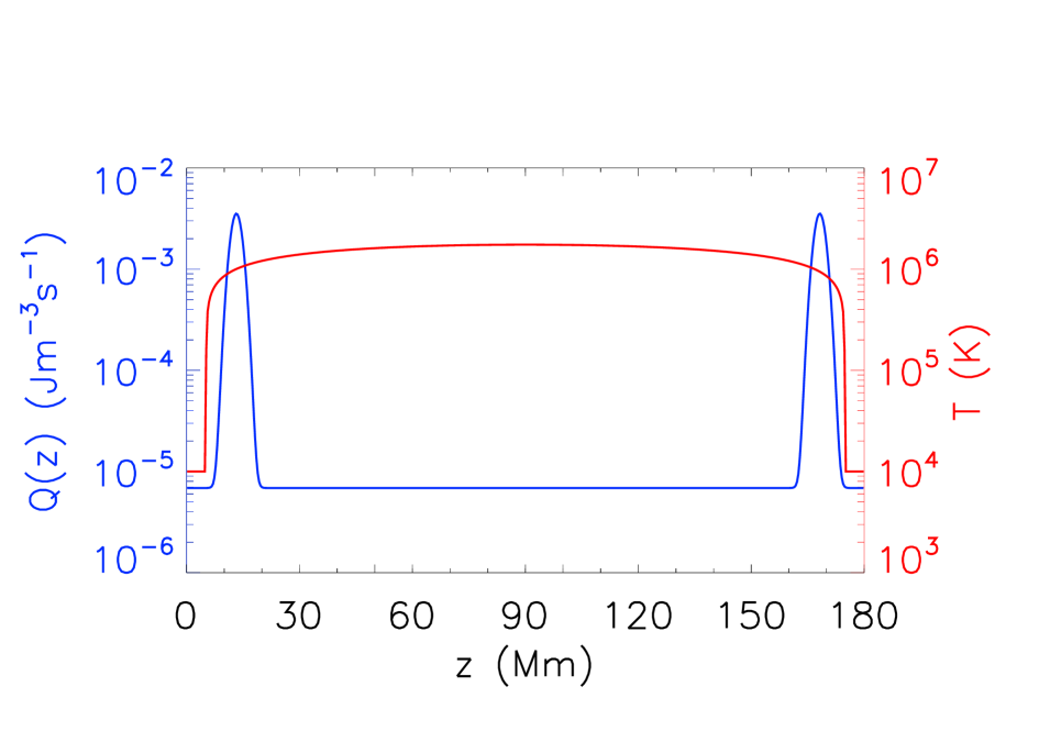
Figure 1: Steady footpoint heating profile $Q(z)$ (blue line, left-hand axis) used in Sections 2.2 and 2.2.2, imposed on top of the temperature initial condition (red line, right-hand axis). The temperature is determined by the imposed background heating.

Figure 2: Influence of numerical resolution on the loop temperature and TNE cycle evolution for steady footpoint heating using HYDRAD simulations. Each plot shows the spatial dependence of temperature (horizontal axis) and the temporal evolution (vertical axis). The various panels represent different values of RL, as indicated above the panel.

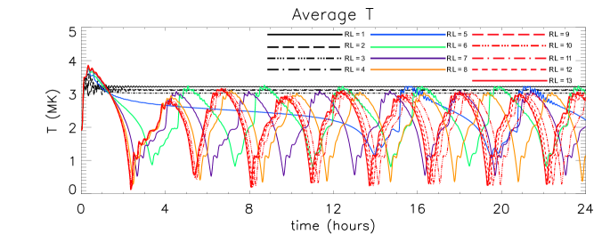
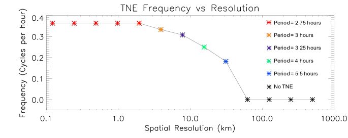
Figure 3: The top three panels show the coronal averaged temperature, density and pressure as a function of time, for thirteen values of RL. The lowest panel shows how the TNE cycle frequency depends on the minimum permitted spatial resolution (coarser resolution is associated with smaller RL). The lines in the upper three panels are colour-coded in a way that reflects the period of the TNE cycle.

Figure 4: Effect of obtaining the correct evaporative response on TNE cycles. Results for steady footpoint heating. The panels show the time evolution of the temperature as a function of position along the loop obtained in two different simulations, each run with the same spatial resolution of 500 grid points along the length of the loop (coarse resolution - 360 km). The left and right-hand panels correspond to the Lare1D and LareJ (Lare1D with the UTR jump condition method) solutions, respectively. On the right of the 2D plots, we display the evolution of the coronal averaged temperature (computed by spatially averaging over the uppermost 25% of the loop).

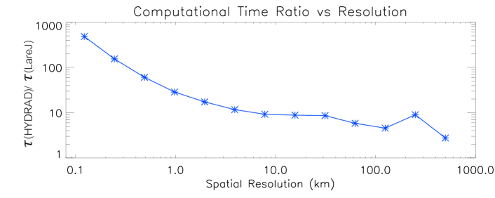
Figure 5: Numerical simulation computation times (run on a single processor) for steady footpoint heating. The panel shows the computational time ratio between HYDRAD and LareJ (Lare1D with 500 grid points and the UTR jump condition method) as a function of the HYDRAD spatial resolution for the different RL runs.

2.2.1 Steady footpoint heating: HYDRAD simulations

Representative of the conditions necessary to induce TNE in coronal loop models (e.g. Müller et al. 2003; Antolin et al. 2010; Peter et al. 2012; Mikić et al. 2013; Froment et al. 2018), we first consider the case of steady footpoint heating where the spatial profile is given by the sum of two Gaussian peaks (one at each loop leg), each defined as,

$$Q_{H}(z)=Q_{H_{0}}\exp\left(\dfrac{-(z-z_{0})^{2}}{2z_{H}^{2}}\right).$$ (1)

These peaks are localised between the base of the corona and base of the TR with a maximal value at $z=12.5$ Mm and we take $z_{H}=1.5$ Mm as the length scale of heat deposition. This is shown in Figure 1 as the blue curve. We note that in this part of the paper a small spatially uniform background heating term is always present so that $Q(z)=Q_{bg}+Q_{H}(z)$. This is commonly done in 1D loop models to ensure that $T$ and $n$ remain positive: here $Q_{bg}=6.8682\times 10^{-6}$ Jm^-3s^-1 and the effect of including a range of values of $Q_{bg}$ will be examined in Section 2.4. Moreover, in order to avoid unrealistic pile up of condensations at the loop apex due to the symmetry of the model, the spatial symmetry of the heating profile is perturbed by adding a small enhancement of 0.4% to the Gaussian peak at the left-hand leg of the loop. The initial state of the loop is determined using just $Q_{bg}$, leading to a temperature of order 1 MK. The footpoint heating is then ramped up linearly over 30 s to a constant value with a peak of $Q_{bg}+Q_{H_{0}}$ with $Q_{H_{0}}=3.5\times 10^{-3}$Jm^-3s^-1. This gives a maximum temperature of approximately $3.5$ MK (a similar energy input and loop length as Models 1 and 2 in Mikić et al. 2013).
We run the HYDRAD code in single fluid mode and perform the steady footpoint heating simulations for a sequence of refinement levels: RL = [1, 2, 3, 4, 5, 6, 7, 8, 9, 10, 11, 12, 13]. This corresponds to grid sizes that range from 500 km for one level of refinement (RL=1) down to 122 m in the case of maximum refinement (RL=13).
The results are shown in Figure 2. Each panel shows the temperature as a function of position (horizontal axis) at a sequence of times (vertical axis). The temporal snapshots are shown every 54 seconds. The refinement levels are indicated above each panel, and increase going from upper left to lower right. The simulations are identical in all respects except for the value of RL. [We note that RL = 3, 10, 11 and 12 are not shown.] There are major differences in the evolution as RL increases. The cases with RL=[1, 2, 4] settle to static equilibria while for RL=[5, 6, 7, 8] there is TNE with condensations, but in each case the cycles have a different period ranging from 5.5 to 3 hours. Convergence of the TNE cycle period and thermodynamic evolution (i.e. the same temperature and density extrema) is seen only for $\textrm{RL}\geq 9$, thus requiring a TR grid resolution of 1.95 km or better.
Figure 3 shows the temporal evolution of the coronal averaged temperature ($T$), density ($n$) and pressure ($P$) for all the values of RL (upper three panels) and the dependence of TNE cycle frequency on the minimum spatial resolution (lowest panel). The coronal averages are calculated by spatially averaging over the uppermost 25% of the loop. These quantities are particularly useful for demonstrating the range of coronal responses obtained in the thirteen simulations run with different values of RL and the periods of the TNE cycles are estimated from the troughs in the coronal averaged temperatures. In the upper three plots each value of RL is associated with a specific colour that we associate with a particular cycle period: these colours can also be seen in the star symbols in the lower panel. For example, the red lines and stars correspond to simulations where the TNE cycle evolution has a period of 2.75 hours (and the various RL values within this group are separated by different line styles). This Figure confirms the earlier conclusion of the importance of adequate resolution on obtaining the correct TNE cycle behaviour. Even if computationally one can achieve a TR resolution of 10 km, then an error in the cycle period of order 20% is still to be expected.
We now turn our attention to understanding why the loops computed with different levels of spatial resolution show such significant inconsistencies in their temporal evolution. We start by considering the first TNE cycle of the RL=13 loop. For the first 30 minutes, the temperature and density in the corona both increase in response to the ramped up footpoint heating, the density by the usual evaporation process (Antiochos & Sturrock 1978; Klimchuk et al. 2008; Cargill et al. 2012a). The subsequent evolution follows the familiar TNE pattern with the temperature falling quite rapidly from 3.9 MK to $10^{4}$K between 30 and approximately 150 minutes, during which time the coronal density continues to increase. The rapid cooling is driven locally by the thermal instability and leads to the formation of the condensation at the loop apex, as found by others (e.g. Müller et al. 2003, 2004, 2005; Mok et al. 2008; Antolin et al. 2010; Susino et al. 2010; Peter et al. 2012; Lionello et al. 2013a; Mikić et al. 2013; Susino et al. 2013; Mok et al. 2016; Froment et al. 2018). The condensation has a peak density of around $14\times 10^{15}$ $\rm{m}^{-3}$ at 195 minutes but then quickly falls down the right-hand leg of the loop. After 195 minutes, the coronal density decreases due to the draining of the ‘condensed’ plasma back into the TR and chromosphere. After this stage, the coronal plasma is reheated and coronal temperatures re-reached. The TNE cycle then repeats with a period of about 2.75 hours. We note though that the coronal temperature and density oscillate throughout the evolution (upper panels of Figure 2) due to the shock waves that are generated during the formation of the condensation and when the mass associated with the condensation falls down the loop leg (Müller et al. 2003, 2004).
The examples with RL=[9, 10, 11, 12] all behave in an identical way, while though RL = [7,8] show differences in the cycle period, the error in the density and temperature when averaged over a cycle are just 7% and 3% respectively.
In contrast, the behaviour of the loop computed with one level of refinement (RL=1, 500 km resolution) is completely different. Initially, the temperature in the corona increases but the evaporative response is significantly underestimated. Rather than passing through the TR continuously in a series of steps, the heat flux jumps across the TR. The incoming energy is then strongly radiated (BC13), leaving little residual heat flux to drive the upflow. Therefore, the lack of spatial resolution leads to an enthalpy flux and coronal density that are artificially low for the prescribed heating profile. This ensures that the loop remains thermally stable. The outcome is that after a transient phase of around 1 hour, the loop settles to a static equilibrium with a coronal temperature and density of 3.2 MK and $0.4\times 10^{15}$ $\rm{m}^{-3}$, respectively. The loops calculated with RL=[2, 3, 4] all show broadly similar behaviour while RL = 5 and 6 are transition cases.

Table 1: A summary of the parameter space used and results from the time dependent footpoint heating cases computed with LareJ.

Case	$t_{d}$	$t_{w}$	$Q_{H_{0}}$	Behaviour	TNE Cycle	Heating Cycle
	(s)	(s)	factor		Period (hrs)	Period (s)
1	62.5	62.5	2	TNE with condensations	2.25	125
2	125	125	2	TNE with condensations	2.5	250
3	250	250	2	TNE with condensations	2.75	500
4	500	500	2	TNE with condensations	2.75	1000
5	1000	1000	2	TNE with condensations	3.0	2000
6	2000	2000	2	TNE with condensations, global cooling & draining	3.5	4000
7	4000	4000	2	Global cooling & draining	-	8000
8	8000	8000	2	Catastrophic cooling with global cooling & draining	-	16000
9	125	375	4	TNE with condensations	3.25	500
10	250	750	4	TNE with condensations	3.25	1000
11	500	1500	4	TNE with condensations, global cooling & draining	3.5	2000
13	1000	3000	4	Global cooling & draining	-	4000
13	2000	6000	4	Global cooling & draining	-	8000
14	125	875	8	TNE with condensations	3.75	1000
15	250	1750	8	Global cooling & draining	-	2000
16	500	3500	8	Global cooling & draining	-	4000

Figure 6: Effect of heating timescales on TNE cycles. LareJ results for time dependent footpoint heating Cases 1–8 together with the steady footpoint heating result. The panels show the time evolution of the temperature as a function of position along the loop.

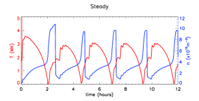
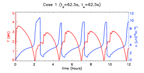
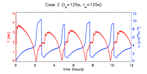
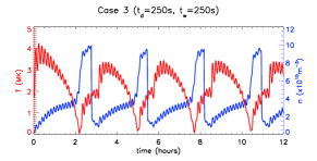
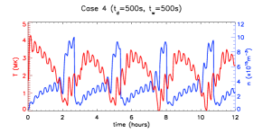
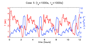
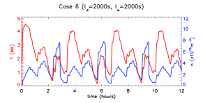
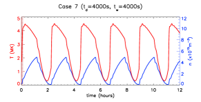
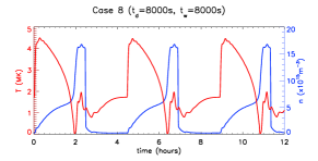
Figure 7: Effect of heating timescales on TNE cycles. LareJ results for time dependent footpoint heating Cases 1–8 together with the steady footpoint heating result. The panels show the time evolution of the coronal averaged temperature (red line, left hand axis) and density (blue line, right hand axis).

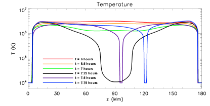
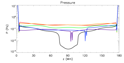
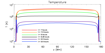
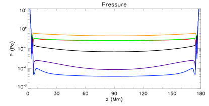
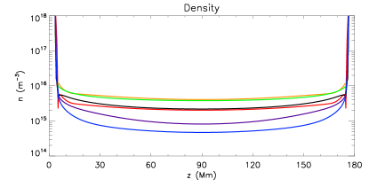
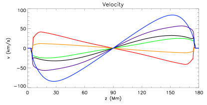
Figure 8: Effect of heating timescales on TNE cycles. LareJ results for time dependent footpoint heating Cases 2 (upper four panels) & 7 (lower four panels). The panels show time ordered snapshots of the temperature, pressure, density and velocity as functions of position along the loop for times during the third TNE cycle of Case 2 and fourth heating cycle of Case 7.

Figure 9: Effect of the background heating on TNE cycles. LareJ results for time dependent footpoint heating. The 2D plots show the time evolution of the temperature as a function of position along the loop. The various panels represent different values of background heating ($Q_{bg}$). On the right of the 2D plots, we display the evolution of the coronal averaged temperature (computed by spatially averaging over the uppermost 25% of the loop). At the bottom of the 2D plots, we show the time averaged footpoint heating profile (blue line, left-hand axis) imposed on top of the temperature initial condition (red line, right-hand axis).

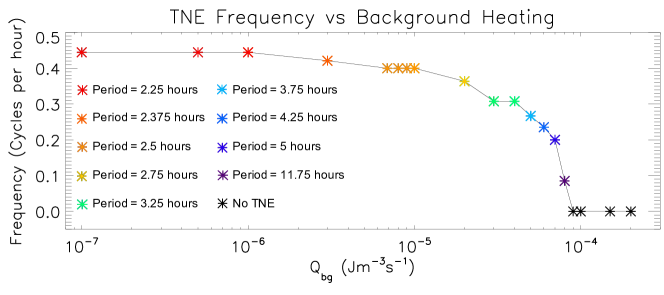
Figure 10: Effect of the background heating on TNE cycles. The panel shows the relation between TNE cycle frequency and the background heating value. Note from Figure 9 that the loop computed with no background heating has a cycle period of 2.25 hours, which is consistent with the asterisk at $Q_{bg}=10^{-7}$ Jm^-3s^-1.

2.2.2 Steady footpoint heating: Lare simulations

We have now shown that with the HYDRAD code adequate TR resolution is required for the correct modelling of footpoint heating and associated TNE, thus extending the result of BC13 which was limited to spatially uniform heating. This suggests that the correct modelling of TNE is unlikely to be a practical proposition in multi-stranded (thousands or more) models of a single observed loop or an entire active region, due to the excessive CPU requirements. Instead, other approaches are required, of which the UTR jump condition method (see Section 2.1) is a well-documented example. We have performed simulations using this approach (referred to as LareJ) for a loop with 500 uniformly spaced grid points and so a resolution of 360 km along the 180 Mm loop. This UTR LareJ approach is compared with the results obtained using the Lare code (referred to as Lare1D) with a coarse spatial of 360 km everywhere. LareJ is considered the benchmark solution because of our prior demonstration of good agreement with HYDRAD (e.g. Johnston et al. (2017a, b)) whereas Lare1D is considered to be representative of a typical simulation with an under-resolved TR.
Figure 4 shows the temporal evolution and spatial variation of the temperature in response to steady footpoint heating, for loops computed with and without the UTR method (LareJ right and Lare1D left respectively). The LareJ approach shows the development of TNE and associated condensations while the Lare1D simulation settles down to a static equilibrium after an initial adjustment to the energy deposition.
The temporal evolution of the coronal averaged temperature from the Lare1D and LareJ loops is shown on the right of each panel in Figure 4. For the Lare1D loop, it is clear that the coronal temperature settles and remains at 3 MK from around 1 hour onwards. On the other hand, the LareJ loop is initially heated to 3.6 MK before locally cooling to $10^{4}$K after 2 hours, in response to an increased coronal density. The evolution then repeats and the loop follows a regular TNE cycle. The period of the cycle is estimated from the troughs in the coronal averaged temperature as about 2.25 hours (three cycles in seven hours from $t=4.5$ hours onwards).
Thus, Figure 4 again demonstrates that the existence of TNE cycles in coronal loop models is strongly dependent on obtaining the ‘correct’ plasma response. This is achieved in LareJ through the UTR approach whereas the Lare1D result is similar to the under-resolved results in Section 2.2.1.
We do note that the TNE cycle period of the LareJ solution is slightly shorter than the fully resolved HYDRAD result and this discrepancy can be attributed to the sources of over-evaporation that are introduced when using the jump condition method (see Johnston et al. (2017b)). However, if we focus on a comparison between Figures 2 and 4, LareJ agrees qualitatively with the converged HYDRAD runs with only minor differences quantitatively, despite under-resolving the TR. The errors in the averaged density and temperature are just 3% and 4% respectively (over a TNE cycle). This has the potential to be of great importance in (a) surveying the large parameter space associated with TNE (e.g. Froment et al. 2018) and (b) modelling TNE in active region simulations with multiple loop strands.
We note also that the UTR method operates only at the footpoints, not at the hot-cool transition at the edge of the condensation. The simulations remain accurate at these locations because the plasma cools largely in situ with no flow through the interface.
Figure 5 summarises the CPU requirements of HYDRAD for all of the values of RL, and demonstrates the large decrease in CPU time of the UTR method (LareJ) over HYDRAD in the simulations where convergence of the TNE cycle period is observed ($\textrm{RL}\geq 9$). In particular, LareJ required at least one order of magnitude less computational time than HYDRAD run with nine levels of refinement (i.e. $\tau(\textrm{HYDRAD[RL=9])}/\tau(\textrm{LareJ})=18$). This is comparable to the improvements in run time described in Johnston et al. (2017a). Therefore, in the remainder of this paper to exploit the short computation time and because the general trends remain the same (i.e. the results are not method dependent), we use LareJ as a reference solution to explore the effects of heating timescales and background heating.

2.3 Effect of heating timescales

In this Section we explore the changes to TNE brought about by unsteady footpoint heating. The heating ($Q_{H}$) is modified by assuming a time-dependent cycle comprising of a series of energy releases each lasting $t_{d}$ seconds, throughout which the maximum footpoint heating rate ($Q_{H_{0}}$) is constant, with a waiting time between these heating events lasting $t_{w}$ seconds when there is no footpoint heating (i.e. $Q_{H}=0$). The background heating remains turned on during the waiting time. Thus:

$$Q(z,t) =Q_{bg}+Q_{H}(z),\quad 0<t<t_{d};$$ (2)

$$Q(z,t) =Q_{bg},\quad t_{d}<t<t_{d}+t_{w},$$ (3)

and so the cycle repeats over $t_{d}+t_{w}$ seconds.
The spatial footpoint heating profile is the same as in Section 2.2. However, we require that the total energy released is the same in all simulations when averaged over a heating cycle, and is equivalent to the steady footpoint heating simulations described previously. Thus the peak heating rate ($Q_{H_{0}}$) in each simulation is increased by a factor $(t_{d}+t_{w})/t_{d}$.
The time-dependent footpoint heating cases are summarised in Table 1 and include short and long heating pulses as well as a range of the ratios $t_{w}/t_{d}$. The former ranges between 62.5 and 8000 seconds and the latter between one and seven. We selected the values used for the unsteady footpoint heating timescales, $t_{d}$ and $t_{w}$, based on current coronal nanoflare models. An upper limit of a few thousand seconds has been suggested for the waiting time (e.g. Cargill 2014; Klimchuk 2015; Marsh et al. 2018). Thus this range is encompassed for $t_{w}$ but the nanoflare duration ($t_{d}$) is more problematic. Some authors believe that $t_{d}$ is short (tens of seconds) while others that it is long (hundreds of seconds e.g. Klimchuk et al. 2008). Hence, we consider a large range for $t_{d}$ due to the uncertainty on the real value.
Figures 6 and 7 show the results for Cases 1 – 8 in Table 1, with steady footpoint heating shown for reference in the upper left panel. Figure 6 shows the loop temperature as a function of position (horizontal axis) and time (vertical axis) and Figure 7 the coronal averaged temperature (red) and density (blue) as a function of time. The former provides both spatial and temporal information to correlate while the latter allows a comparison between the coronal properties around the loop apex (between $z=67.5$ Mm and $z=112.5$ Mm) as a function of time. In particular, the phasing between the coronal averaged temperature and density is used to identify the characteristic behaviour of the simulations (e.g. TNE has peak density at the time of the temperature minimum).
There are two regimes evident, one exists for short and long heating pulses and the other for intermediate values, although there is also overlap between them. The fifth column of Table 1 provides a concise summary. For short $t_{d}$ and $t_{w}$ (up to $t_{d}=500s$) the properties are similar to steady heating, with TNE occuring and determining the cyclic behaviour of the loop evolution. However, superposed on top of this behaviour is a jaggedness in both $T$ and $n$ associated with the impulsive heating.
For longer $t_{d}$ and $t_{w}$ the behaviour changes, with the TNE cycle becoming less evident and the loop cyclic evolution being essentially the same as the heating cycle and, by $t_{d}=4000$ s, there is a transition to a loop that undergoes a heating and cooling cycle, but without evidence of TNE and catastrophic cooling (we refer to this as ‘global cooling’ to indicate the absence of the very localised cool and dense regions characteristic of TNE). The loop cyclic evolution in these cases is entirely determined by the heating cycle. Such global cooling is the behaviour seen with ‘intermediate’ and ‘low-frequency’ coronal nanoflares (e.g. Cargill 2014; Cargill et al. 2015).
However, for very large $t_{d}$, catastrophic cooling from the thermal instability returns and occurs prior to global cooling, without the cyclic character of TNE but with the loop evolution determined by the heating cycle. The last two panels of Figure 7 make this point well: panel 8 shows global cooling (or nanoflare-like response) and panel 9 catastrophic cooling with global cooling.
The different regimes are highlighted further in Figure 8 with the upper and lower panels showing a series of snapshots of $T$, $P$, $n$ and $v$ for Cases 2 ($t_{d}=125$ s) and 7 ($t_{d}=4000$ s) respectively. For Case 2, the evolution is, despite the bursty nature of the heating, representative of TNE as discussed in the literature. Thus the 250 s cycle of the heating, being shorter than the characteristic time for TNE to evolve, plays no significant role. On the other hand, Case 7 shows evolution characteristic of an impulsively-heated loop (e.g. Klimchuk 2006) with a rise in temperature, followed by the density increase due to evaporation, then, after the time of maximum density, an enthalpy and radiative global cooling phase (Bradshaw & Cargill 2010b). In this case, the heating is turned on for just over one hour and thermal instability does not have time to develop before the heating declines. In other words, the density due to the evaporation is limited to a value below that needed for thermal instability.
Figure 8 also demonstrates that TNE in the corona (upper four panels) can be characterised by quantities such as the skew and flatness. This is clear from the top left-hand panel where the temperature evolution between 6.5 and 7.25 hours shows both developing. In contrast, the low frequency nanoflare-like response (lower four panels) does not show this type of behaviour.
It is also interesting to note that for Case 8, there is a return to thermal instability, and the TNE cyclic evolution would return if the heating was kept for longer times. Here the heating pulse is long enough for the loop to see it as being ‘steady’, so that the density in the corona is large enough for thermal instability (and the corresponding catastrophic cooling) to set in.
For cases 1 - 8, the transition between the TNE cycle and the heating (and global cooling) cycle occurs roughly when $t_{d}=t_{w}=2000$ s with the 4000 s cycle roughly being equal to the characteristic time for thermal instability onset (and subsequent TNE cycle), with a partial transition back to catastrophic cooling for Case 8. Cases 9 - 16 reinforce our conclusions with TNE occurring only for short pulse cycles.
However, within this general classification, there are some subtleties when we switch between the two types of characteristic behaviour. This transition takes place when the waiting time ($t_{w}$) between heating periods becomes comparable to the loop cooling time. The outcome is a mixed regime which is characterised by properties that incorporate both types of behaviour. For example, Cases 6 and 11 exhibit catastrophic cooling from the triggering of the thermal instability and global cooling from the ending of the heating pulse. These cases have waiting times of 2000 s and 1500 s, respectively.
We stress that these examples are limited in that strong symmetry is assumed both with the intensity and time variability of the heating at both footpoints. While the breaking of this symmetry could lead to new forms of behaviour such as siphon flows (e.g. Cargill & Priest 1980; Mikić et al. 2013; Froment et al. 2018), the dependence of the loop evolution on time-variability of the heating can be expected to persist.

2.4 Effect of the background heating

Next we investigate the effect of the background heating on the TNE cycle evolution. The background heating ($Q_{bg}$) is varied over several orders of magnitude, ranging from no background heating up to $10^{-4}$ Jm^-3s^-1. All other parameters are as in previous Sections, the footpoint heating uses the values of Case 2 in Section 2.3 and LareJ results are shown.
Figure 9 shows the evolution of the temperature, as a function of time and position along the loop with $Q_{bg}=$ [0, 6.8682$\times 10^{-6}$, 2$\times 10^{-5}$, 4$\times 10^{-5}$, 6$\times 10^{-5}$, $10^{-4}$] Jm^-3s^-1 in the six panels. The sum of the spatial distribution of the footpoint heating at the peak of the heating cycle and the background heating (blue) are shown below each panel. For reference we note that $Q_{bg}=6.8682\times 10^{-6}$ Jm^-3s^-1 corresponds to the minimum value required to achieve thermal balance in the hydrostatic initial condition and will be referred to as the equilibrium background heating value. Furthermore, $Q_{bg}=6\times 10^{-5}$ Jm^-3s^-1 was previously used as the background heating value in the Model 1 heating profile that was considered by Mikić et al. (2013).
Figure 9 shows that five of the loops experience TNE with condensations but the cycle periods (and thermodynamic evolution during a cycle) are significantly different. For example, the case with ‘equilibrium’ background heating value has a TNE cycle period of 2.5 hours, while increasing $Q_{bg}$ to $6\times 10^{-5}$ Jm^-3s^-1 increases the period to 4.25 hours. Moreover, for no background heating the period is 2.25 hours. We also note that the case with the largest background heating ($Q_{bg}=10^{-4}$ Jm^-3s^-1), is stable to the thermal instability and instead settles to a static equilibrium.
Figure 10 shows the range of TNE cycle periods obtained for all of the background heating runs. Convergence to a period of 2.25 hours is only observed for small background heating values ($Q_{bg}\leq 10^{-6}$ Jm^-3s^-1) while loops computed with $Q_{bg}\geq 9\times 10^{-5}$ Jm^-3s^-1 do not experience TNE.
The suppression of TNE arises as $Q_{bg}$ increases because for it to occur, the radiative losses must exceed the heating in the corona. Obviously as $Q_{bg}$ increases, this becomes more difficult. Therefore, triggering the thermal instability when an increased background heating value is used requires either (i) an extended heating duration or (ii) an increase in the magnitude of the maximum footpoint heating rate ($Q_{H_{0}}$) in order to accumulate a sufficient amount of mass in the corona. The influence of the latter is observed as the suppression of TNE cycles when the footpoint heating rate is not increased relative to background heating rate while the effect of the former is seen as an increase in the TNE cycle period. We can thus conclude that the ratio of the maximum footpoint heating rate to the background heating value plays a key role in the onset criteria for TNE.

3 Discussion and conclusions

The phenomenon of TNE is a very challenging one for numerical models for several reasons, in particular the need to correctly resolve the TR and so sustain precise periodicity and thermodynamic characteristics of the coronal condensations. We have shown that inadequate TR resolution can lead to incorrect properties of the TNE cycles and even the suppression of TNE. An approximate method of handling the TR is shown to eliminate this problem with the benefit of significantly shorter computational times while introducing a small discrepancy of order 15% in the condensation periodicity. Furthermore, when averaged over a TNE cycle, the error in the coronal density and temperature evolution is only 3% and 4% respectively.
The approximate method is applied to models of TNE with steady, uniformly distributed ‘background’ heating as well as unsteady footpoint heating. In the former case we find a trend evident in previous work (e.g. see Models 1 and 2 in Mikić et al. 2013), namely that TNE in a loop with footpoint heating is suppressed unless the background heating is sufficiently small. Such a small steady background heating is sometimes included in models for computational reasons (e.g. Section 2) and a physical motivation is currently unclear. However, any background heating need not be steady for TNE to be suppressed. For example high frequency coronal nanoflares (Warren et al. 2011; Cargill et al. 2015) would achieve this, as discussed in Antolin et al. (2010), where the dissipation of torsional finite-amplitude Alfvén waves by shock heating (Antolin et al. 2008) eliminates the TNE cycles present in a footpoint heated loop and leads instead to a uniformly heated loop in thermal equilibrium.
On the other hand, a background of low frequency coronal nanoflares (Cargill et al. 2015) are sufficiently infrequent that TNE can proceed superimposed on their behaviour (although they may increase the resulting period of the loop’s cyclic evolution). Intermediate frequency nanoflares, now widely believed to be responsible for active region heating (Cargill 2014; Barnes et al. 2016; Viall & Klimchuk 2017) repeat on the loop cooling time, so that results similar to those shown in Section 2.4 will be found.
Unsteady footpoint heating leads to further complications. For heating bursts of a specified duration separated by a waiting time, thermal instability arises for both short and very long (¿ 6000 s) heating times. Cyclic evolution is given by the TNE cycle for the short heating times and by the heating cycle itself for the longer. In addition, a new intermediate regime of mixed catastrophic cooling from thermal instability and global cooling from the cessation of heating arises for waiting times of order a few thousand seconds and is comparable to the behaviour of a corona heated by low-frequency nanoflares.
When the condensation dynamics are considered, important differences arise that can help distinguish this intermediate regime in observations. During a TNE cycle the speed of a falling condensation is determined by its mass and by the surrounding coronal gas pressure (Antolin et al. 2010; Oliver et al. 2014). Instead, condensations occur along with global cooling, so that the coronal pressure drops as the condensations fall, thus rapidly increasing their speeds with accelerations tending to the gravitational value. Coronal rain is usually observed to fall with an acceleration lower than due to gravity along a curved loop (Schrijver 2001; De Groof et al. 2004; Antolin et al. 2012; Antolin & Rouppe van der Voort 2012), although the observed distribution of speeds for the rain has a long tail towards higher values. These results suggest a broad range of possible TNE evolution depending on the waiting time but one that in an average sense does not correspond to the intermediate regime.

3.1 Parametric dependence of TNE

To conclude this paper, we address two points that seem to be essential in advancing the topic of TNE in coronal loops. Clearly there is a complex relation between the onset of TNE as various footpoint heating parameters are varied. While models of TNE predict generic global and local features in spectral diagnostics of the solar corona including loops undergoing a cyclic heating and cooling evolution of evaporation and condensation, the existence of these cycles depends on several parameters (e.g. Antiochos et al. 2000; Karpen et al. 2001; Müller et al. 2003, 2004, 2005; Mendoza-Briceño et al. 2005; Mok et al. 2008; Antolin et al. 2010; Susino et al. 2010; Lionello et al. 2013a; Mikić et al. 2013; Susino et al. 2013; Mok et al. 2016) which include (but need not be limited to) geometrical factors (such as the loop length and area expansion) and the nature of the heating mechanism (its spatial and temporal distribution, the degree of asymmetry between both footpoints, its stochasticity and so on). As shown by Froment et al. (2018) the existence of TNE cycles seem to be very sensitive to some of these parameters, suggesting that if they are approximately uniformly distributed, the vast majority of loops should not exhibit TNE.
Assuming that loops consist of independently heated strands (and therefore undergo an independent thermodynamic evolution) Klimchuk et al. (2010) have shown that the TNE theory leads to inconsistencies with observational constraints for the solar corona (see also Klimchuk 2015). While TNE does seem to explain very well loops with coronal rain (Mok et al. 2008; Kamio et al. 2011; Peter & Bingert 2012; Antolin et al. 2010; Antolin & Rouppe van der Voort 2012; Antolin et al. 2015; Fang et al. 2013, 2015, 2016) and loops exhibiting highly periodic EUV intensity pulsations (Auchère et al. 2014; Froment et al. 2015, 2018; Auchère et al. 2018), it is unclear how much of the coronal volume is involved in these phenomena. Recent numerical work has shown that by varying some of the above mentioned parameters (Mikić et al. 2013; Froment et al. 2018; Winebarger et al. 2018) and including multi-dimensional effects (Lionello et al. 2013b; Mok et al. 2016; Winebarger et al. 2016; Xia et al. 2017) some of the difficulties may be resolved.
Thus the large parameter space involved in the existence of TNE constitutes a challenge for disentangling the properties of the underlying heating. As a further example, in our parameter space investigation we have produced loops with very similar global parameters (TNE cycle period, average coronal density and temperature, siphon flow velocities and so on) but with significant variation in the amount of heating input (a factor of one third to one half). Caution must therefore be placed on using only one of these proxies (such as the TNE cycle period) rather than the ensemble of observational constraints, both at a global and local level (for instance, regarding the dynamics of condensations and their observational signatures).

3.2 Footpoint heating

Many results have shown that the presence of TNE requires footpoint heating. It is thus pertinent to ask what the direct evidence for such localised heating actually is. One can dismiss the idea that the heating is strictly steady: that is not how plasmas release energy, yet many models impose just such a condition. However, as we have shown, high frequency bursty heating does approximate steady heating.
Direct observational evidence for footpoint heating is limited (e.g. Hara et al. 2008; Nishizuka & Hara 2011; Testa et al. 2014), the latter being interpreted as the footpoint response to a coronal acceleration of electrons. Further, observations of spicules suggest that associated heating to coronal temperatures along with nonthermal line broadenings and upflows all arise in the lower solar atmosphere (e.g. De Pontieu et al. 2011; Martínez-Sykora et al. 2018). Whether this corresponds to adequate footpoint heating is unclear, but it has been suggested that minimal coronal heating in fact results (e.g. Klimchuk 2012). Studies of TNE where both its coronal manifestation and spectral observations at the footpoints are thus an essential future requirement.
A number of theoretical models also give results where heating is concentrated at the base of loops. These include ‘braiding’ type models (e.g. Gudiksen & Nordlund 2005) and turbulent cascades due to interacting Alfven waves (e.g. van Ballegooijen et al. 2011). However, apart from limited numerical resolution, such models also include unrealistically high dissipation coefficients, in part to avoid numerical instabilities, which can lead to a lack of ability to resolve fine-scale currents. A consequence of this is an effectively (temporally) constant coronal heating background which may also be in the wrong place due to the lack of ability to model the small-scale current structure throughout the atmosphere. The problem confronting such models is compounded by the difficulty of TR resolution.
On the other hand, models that do better in resolving such currents (e.g. Bareford & Hood 2015) do not attempt to model the transition between chromosphere and corona, so cannot address the question of footpoint heating. Thus it seems evident that details of the ‘what, where or why’ of footpoint heating are very unclear at this time.
A further important result from this series of papers (Johnston et al. 2017a, b) and previous work (Bradshaw & Cargill 2013) is that intensities of coronal lines may not be realistic simply because of the wrong evaporative response of the atmosphere to the heating input due to the limited numerical resolution. This is particularly likely to be a problem in 3D MHD models. The present work also suggests that, besides coronal lines, TR and chromospheric lines may also be affected since TNE cycles and the accompanying coronal rain (which have strong signatures in chromospheric, transition region and EUV lines) may be far more common than previously thought in more realistic global 3D MHD models (and as suggested by observations). Thus approximate methods such as presented here and by Mikić et al. (2013) are vital for large-scale contemporary MHD models since they can ‘free up’ grid points which can then be used to resolve better the currents responsible for the heating. However, their extension to 3D MHD requires a more sophisticated treatment than in 1D, in particular how the magnetic field and transverse velocity modify the jump relations.