Individual dipole toroidal states: main features and search in $(e,e^{\prime})$ reaction

Abstract

Individual low-energy E1 toroidal and compressional states (TS and CS) produced by the convective nuclear current ${\bf j}_{\rm c}$ were recently predicted for ²⁴Mg in the framework of quasiparticle random-phase-approximation (QRPA) with Skyrme forces. In the present QRPA study with Skyrme parametrization SLy6, we explore in more detail properties of these states (toroidal and compressional responses, current distributions, and transitions probabilities $B(E1K,0^{+}0\to 1^{-}K),\;B(E3K,0^{+}0\to 3^{-}K)$, $B(M2K,0^{+}0\to 2^{-}K)$ with $K=$0 and 1) and analyze the possibility to discriminate and identify TS in inelastic electron scattering to back angles. The interplay of the convective $\mathbb{j}_{\rm c}$ and magnetization $\mathbb{j}_{\rm m}$ nuclear currents is thoroughly scrutinized. A two-step scheme for identification of TS in $(e,e^{\prime})$ reaction is proposed. The key element of the scheme is the strong interference of the orbital and spin contributions, resulting in specific features of E1 and M2 transversal form factors.

I Introduction

In our recent publications, individual low-energy E1 toroidal and compressional states (TS and CS) in deformed nuclei ²⁴Mg Ne_PRL18 and ²⁰Ne Ne_20Ne were predicted within the quasiparticle random-phase-approximation (QRPA) method with Skyrme forces. In ²⁴Mg, the TS is predicted to appear as the lowest (E=7.92 MeV) dipole state with K=1 (where K is the projection of the total angular momentum to the symmetry z-axis). Comparable individual low-energy dipole TS were found for ¹⁰Be KE10Be_PRC17 ; KE10Be_arXiv19 , ¹²C KE12C_PRC18 , and ¹⁶O KE16O_arXiv19 using the combined antisymmetrized molecular dynamics and generator coordinate method KE_rew18 . These predictions open a new promising path for the exploration of vortical toroidal excitations. Previously, the nuclear toroidal mode was mainly studied as E1 isoscalar (T=0) toroidal giant resonance (TGR), see e.g. Se81 ; Bas93 ; Mis06 ; Balb94 ; Ry02 ; Co00 ; Vr02 ; Pa07 ; Kv11 ; Rep13 ; Rei14 ; NePAN16 ; Rep17 and references therein. However the experimental observation and identification of the TGR is hampered by serious troubles. The resonance is usually masked by other multipole modes (including dipole excitations of non-toroidal nature) located in the same energy region. As a result, even the most relevant $(\alpha,\alpha^{\prime})$ experimental data YoungexpZr ; Uch04 still do not provide the direct evidence for E1 TGR, see the discussion in Ref. Rep17 . In this connection, individual low-energy E1 TS in light nuclei have obvious advantages in exploration of the toroidal mode. They are well separated from the neighbor dipole states and so can be easier discriminated and identified in experiment than the TGR.

In this paper, we present a thorough exploration of various features of TS and CS in ²⁴Mg. In addition to TS at 7.92 MeV, the toroidal E1(K=1) excitation at 9.97 MeV is analyzed. The special attention is paid to the impact of the magnetization nuclear current $\mathbb{j}_{\mathrm{m}}$ which, being vortical, can affect the results for customary TS produced by the convective current $\mathbb{j}_{\mathrm{c}}$. It is found that $\mathbb{j}_{\mathrm{m}}$ can cause E1(K=0) TS of predominant magnetization origin. We also show that, similar to recording of the vortical scissors sciss and twist twist modes by strong orbital M1 and M2 transitions, the vortical TS in deformed nuclei can be also signified by enhanced M2 transitions $0^{+}0\to 2^{-}K$ between the ground state and $I^{\pi}K=2^{-}1$ rotational state based on the TS with $I^{\pi}K=1^{-}1$.

It is known that there is a general, yet unresolved, problem how to search and identify vortical nuclear states in experiment. In this connection, we propose a two-step scheme which could be useful in solution of this problem. We apply this scheme to the search for the convective TS in $(e,e^{\prime})$ scattering to backward angles. Since E1 toroidal form factor is transversal Bas93 ; Mis06 , this reaction looks most suitable.

At the first step of the scheme, the appropriate candidates for TS have to be chosen from, e.g., QRPA calculations. These are states with a significant toroidal E1 strength, clear toroidal distribution of the nuclear current, and enhanced $B(M2)$ value. At the second step, the calculated transversal E1 and M2 form factors for these states are compared with experimental $(e,e^{\prime})$ data. Our analysis shows that strong interference of the orbital and spin contributions leads to specific features of E1 and M2 transversal form factors. As a result, these form factors become very sensitive probes for the spin/orbital interplay. So, if $(e,e^{\prime})$ data cannot be described by the spin contribution alone but are well reproduced by spin + orbital contributions, we may conclude that the orbital fraction is essential and correctly produced by the calculations. Then we are confident that the structure of chosen state is valid and its TS character and toroidal distribution of the nuclear current may be considered as established.

The paper is organized as follows. In Sec. II, the calculation scheme is outlined. In Sec. III, the numerical results are presented. The responses, current fields, electromagnetic transitions, and E1 and M2 transversal form factors are discussed in detail. In Sec. IV, the conclusions are drawn.

II Calculation scheme

The calculations for ²⁴Mg are performed within the self-consistent QRPA based on the Skyrme functional Ben03 . As in our earlier studies Ne_PRL18 ; Ne_20Ne , we use the Skyrme parametrization SLy6 SLy6 . The QRPA code for axial nuclei Repcode exploits a 2D mesh in cylindrical coordinates. The single-particle basis includes all the states from the bottom of the potential well up to +55 MeV. The axial equilibrium deformation is $\beta$=0.536 as obtained by minimization of the energy of the system. The volume pairing modeled by contact interaction is treated at the BCS level Rep17 . The QRPA uses a large two-quasiparticle (2qp) basis with the energies up to $\sim$ 100 MeV. The basis includes $\approx$ 1900 ($K=0$) and $\approx$ 3600 (K=1) states. This basis guarantees that the Thomas-Reiche-Kuhn sum rule Ring_book ; Ne08 and isoscalar dipole energy-weighted sum rule Harakeh_book_01 are exhausted by 100$\%$ and 97$\%$, respectively.

The toroidal and compressional modes are coupled Vr02 ; Pa07 ; Kv11 and comparison of these vortical and irrotational patterns of the nuclear flow is always instructive Kv11 . So we inspect both vortical TS and irrotational CS. The toroidal and compressional responses are quantified in terms of reduced transition probabilities

$$B_{\nu}(E1K,\alpha)=(2-\delta_{K,0})|\>\langle\nu|\>\hat{M}_{\alpha}(\;E1K)\>|0\rangle\>|^{2}$$ (1)

where $|0\rangle$ and $|\nu\rangle$ mark the QRPA ground state and excited $\nu$-th dipole state. Matrix elements for the toroidal ($\alpha$=tor) and compressional ($\alpha$=com) transition operators are Kv11 ; Rep13 ; Ne_PRL18

$$\langle\nu|\hat{M}_{\text{tor}}(E1K)|0\rangle$$ (2)

$$=\frac{-1}{10\sqrt{2}c}\int d^{3}rr[r^{2}+d^{s}+d^{a}_{K}]{\bf Y}_{11K}\cdot(\bf{\nabla}\!\times\!\delta{\mathbb{j}}^{\nu}({\mathbb{r}}))\;,$$

$$\langle\nu|\hat{M}_{\text{com}}(E1K)|0\rangle$$ (3)

$$=\frac{-i}{10c}\int d^{3}rr[r^{2}+d^{s}-2d^{a}_{K}]Y_{1K}(\bf{\nabla}\cdot\delta{\mathbb{j}}^{\nu}({\mathbb{r}})),$$

where ${\bf Y}_{11K}(\hat{\bf r})$ and $Y_{1K}(\hat{\bf r})$ are vector and ordinary spherical harmonics; $\delta{\mathbb{j}}^{\nu}({\mathbb{r}})=\langle\nu|\hat{\mathbb{j}}|0\rangle({\mathbb{r}})$ is the current transition density (CTD); $d^{s}=-5/3\langle r^{2}\rangle_{0}$ is the center-of-mass correction (c.m.c.) in spherical nuclei Kv11 ; NVGS81 ; Rep19 ; $d^{a}_{K}=\sqrt{4\pi/45}\langle r^{2}Y_{20}\rangle_{0}(3\delta_{K,0}-1)$ is the additional c.m.c. arising in axial deformed nuclei Rep19 ; YNVG08 . The average values in c.m.c. are $\langle f\rangle_{0}=\int\>d^{3}rf\>\rho_{0}/A$ where $\rho_{0}$ is the g.s. density. As was checked, these c.m.c. accurately remove spurious center-of-mass admixtures in ²⁴Mg.

The operator of the nuclear current

$$\hat{\mathbb{j}}(\mathbb{r})=\hat{\mathbb{j}}_{\rm b}(\mathbb{r})+\hat{\mathbb{j}}_{\rm cdt}(\mathbb{r})$$ (4)

includes the bare current $\hat{\mathbb{j}}_{\rm b}$ BMv1 and the correction $\hat{\mathbb{j}}_{\rm cdt}$ RK19 taking into account the effect of the current-dependent terms in the Skyrme functional. The correction is necessary to recover the continuity equation in Skyrme-QRPA calculations of the responses and form factors. The effect of $\hat{\mathbb{j}}_{\rm cdt}$ is negligible in T=0 responses but can be noticeable in T=1 and mixed cases RK19 .

The bare current consists of the convective and magnetization (spin) parts,

$$\hat{\mathbb{j}}_{\rm b}(\mathbb{r})=\hat{\mathbb{j}}_{\rm c}(\mathbb{r})+\hat{\mathbb{j}}_{\rm m}(\mathbb{r})=\frac{e\hbar}{m}\sum_{q=n,p}(\hat{\mathbb{j}}_{\;\rm c}^{q}(\mathbb{r})+\hat{\mathbb{j}}_{\;\rm m}^{q}(\mathbb{r}))\;,$$ (5)

where

$$\hat{\mathbb{j}}^{q}_{\;\rm c}(\mathbb{r}) = -i\frac{e_{\text{eff}}^{q}}{2}\sum_{k\epsilon q}(\delta({\mathbb{r}}-{\mathbb{r}}_{k}){\mathbb{\nabla}}_{k}+{\mathbb{\nabla}}_{k}\delta({\mathbb{r}}-{\mathbb{r}}_{k})),$$ (6)

$$\hat{\mathbb{j}}^{q}_{\;\rm m}(\mathbb{r}) = \frac{\bar{g}^{q}_{s}}{2}\sum_{k\epsilon q}({\mathbb{\nabla}}_{k}\times\hat{\mathbb{s}}_{qk})\delta({\mathbb{r}}-{\mathbb{r}}_{k}).$$ (7)

Here $\hat{\mathbb{s}}_{qk}$ is the spin operator, $e_{\text{eff}}^{q}$ are effective charges, $\bar{g}^{q}_{s}$ are spin g-factors, $k$ numerates the nucleons. In the present calculations, we use the isoscalar ($e^{\rm n,p}_{\rm eff}=0.5$, $\bar{g}^{\rm n,p}_{s}=(g_{s}^{n}+g_{s}^{p})\eta/2=0.88\eta$) and proton ($e^{\rm p}_{\rm eff}=1,e^{\rm n}_{\rm eff}=0$, $\bar{g}^{\rm n,p}_{s}=\eta g^{\rm n,p}_{s}$) nuclear currents, where $g^{\rm p}_{s}=5.58$ and $g^{\rm n}_{s}=-3.82$ are bare g-factors and $\eta$ =0.7 is the quenching Harakeh_book_01 . The isoscalar current is relevant for the comparison of the responses with data from isoscalar reactions like $(\alpha,\alpha^{\prime})$. The proton current is relevant for $(e,e^{\prime})$ reaction.

The toroidal matrix element (2) with $(\bf{\nabla}\!\times\!\delta{\mathbb{j}}^{\nu}({\mathbb{r}}))$ and compressional matrix element (3) with $(\bf{\nabla}\cdot\delta{\mathbb{j}}^{\nu}({\mathbb{r}}))$ are determined by the vortical and irrotational nuclear flow, respectively. The proton and neutron CTD from the convective and magnetization parts of the nuclear current are $\delta\mathbb{j}^{q}_{\;\rm c}=\langle\nu|\hat{\mathbb{j}}^{q}_{\;\rm c}|0\rangle$ and $\delta\mathbb{j}^{q}_{\;\rm m}=\langle\nu|\hat{\mathbb{j}}^{q}_{\;\rm m}|0\rangle$.

For magnetic quadrupole transitions $0^{+}0\to 2^{-}K$, the reduced transition probability is

$$B_{\nu}(M2K)=(2-\delta_{K,0})|\>\langle\nu|\>\hat{M}(M2K)\>|0\rangle\>|^{2}$$ (8)

with the transition operator

$$\hat{M}(M2K)=\mu_{N}\sum_{q=n,p}\sum_{k\epsilon q}[g_{s}^{q}\hat{\mathbb{s}}_{qk}+\frac{2}{3}g_{l}^{q}\hat{\mathbb{l}}_{qk}]\cdot\mathbb{\nabla}_{k}[r^{2}Y_{2K}]_{k}$$ (9)

where $\hat{\mathbb{l}}_{qk}$ is the operator of the orbital moment, the orbital g-factors are $g_{l}^{q}$=1 for protons and 0 for neutrons.

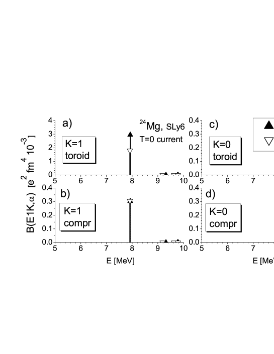
[h]

Figure 1: Toroidal (upper panels) and compressional (bottom panels) B(E1K,$\alpha$)-strengths in ²⁴Mg, calculated with T=0 nuclear current. Calculations with (filled triangles) and without (empty reverse triangles) $\bf{j}_{\rm m}$ are compared.

III Results and discussion

III.1 Toroidal and compression responses, current fields

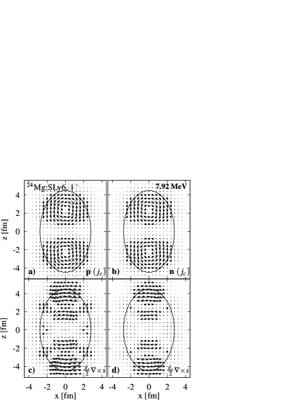
Figure 2: QRPA proton (left) and neutron (right) fields of the convective $\delta\mathbb{j}^{q}_{\rm c}$ (upper plots) and magnetic $\delta\mathbb{j}^{q}_{\rm m}$ (bottom plots) currents in the toroidal 7.92-MeV $K^{\pi}=1^{-}$ state. In (c)-(d), the bare g-factors with the quenching are used.

In Figure 1, the low-energy toroidal and compressional transition strengths (1) in ²⁴Mg are shown. They are calculated with T=0 nuclear current relevant for isoscalar $(\alpha,\alpha^{\prime})$ reaction. The cases with and without $\bf{j}_{\rm m}$, are compared. Plot (a) shows that only the K=1 state at 7.92 MeV exhibits the large toroidal response. The toroidal nature of this state is additionally confirmed by the proton and neutron fields of the convective current, shown in the plots (a)-(b) of Fig. 2. Just this 7.92-MeV state was proposed in Ne_PRL18 as the individual low-energy TS. Due to the large axial quadrupole deformation in ²⁴Mg, the vortical flow of this state is transformed from the familiar toroidal vortical ring into the vortex-antivortex dipole Ne_PRL18 . The 7.92-MeV state is not fully vortical since, following Fig. 1 (b), it has a small compressional irrotational response. Even being small, the irrotational fraction can serve as a doorway for excitation of TS in various reactions. If a reaction cannot generate vortical excitations directly, this can be done indirectly through the irrotational fraction.

Figure 3: As Fig. 2 but for the 9.56-MeV $K^{\pi}=0^{-}$ state.

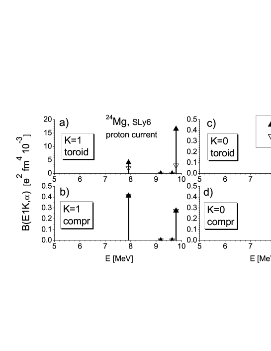
Figure 4: As Fig. 1 but for the proton nuclear current, see text for more detail.

The plots Fig. 1 (c)-(d) show that the compressional strength exceeds the toroidal one for the K=0 state at 9.56 MeV. The convective current $\delta\mathbb{j}^{q}_{\rm c}$ in this state (see Fig. 3 (a)-(b)) resembles the octupole flow for the $3^{-}$ state in ²⁰⁸Pb RW87 . This is not surprising since there is a strong coupling between dipole and octupole modes in nuclei with a large quadrupole deformation, like ²⁴Mg. This coupling should be especially strong in irrotational states like 9.56-MeV one.

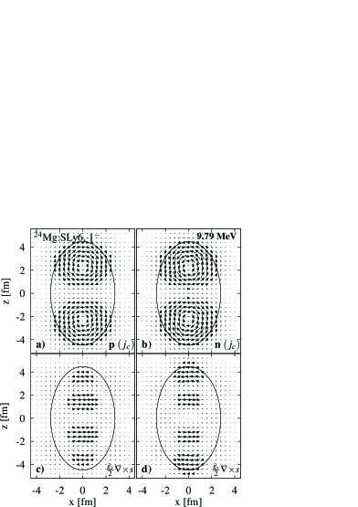
Figure 5: As Fig. 2 but for 9.79-MeV $K^{\pi}=1^{-}$ state.

We now look at the impact of ${\mathbb{j}}_{\rm m}$. As seen from Fig. 1 (plots (b) and (d)), the compressional strengths with and without $\bf{j}_{\rm m}$ are almost the same. This is expected since vortical magnetization current should not affect the irrotational compressional flow. At the same time, plots (a) and (c) of Fig. 1 show that inclusion of ${\mathbb{j}}_{\rm m}$ significantly changes the toroidal strengths: it is increased by $\sim 30\%$ in the K=1 7.92-MeV state and decreased to almost half in the K=0 9.56-MeV state. Thus the impact of ${\mathbb{j}}_{\rm m}$ on the toroidal strength is rather strong.

The proton and neutron magnetization current fields $\delta{\mathbb{j}}^{q}_{\rm m}$ for 7.92-MeV state shown in Fig. 2 (c)-(d) are not toroidal. At the same time, these fields in the K=0 9.56-MeV state, shown in in Fig. 3 (c)-(d), look like toroidal. Thus ${\mathbb{j}}_{\rm m}$, similar to ${\mathbb{j}}_{\rm c}$, can cause a toroidal flow, which proves that magnetization vortical TS can exist.

Table 1: Main two-quasiparticle (2qp) components $ii^{\prime}$ (denoted by Nilsson asymptotic quantum numbers $Nn_{z}\Lambda$) in some low-energy dipole $\nu$-states in ²⁴Mg. For each component, the forward amplitude $X^{\nu}_{ii^{\prime}}$ and contribution $N^{\nu}_{ii^{\prime}}$ to the state norm are listed.

E [MeV]	K	main 2qp components	$X^{\nu}_{ii^{\prime}}$	$N^{\nu}_{ii^{\prime}}$
7.92	1	pp[211$\uparrow$-330$\uparrow$]	0.73	0.54
		nn[211$\uparrow$-330$\uparrow$]	0.62	0.39
9.56	0	pp[211$\downarrow$-101$\downarrow$]	0.62	0.39
		nn[211$\downarrow$-101$\downarrow$]	0.56	0.31
9.79	1	nn[211$\uparrow$-330$\uparrow$]	-0.74	0.55
		pp[211$\uparrow$-330$\uparrow$]	0.65	0.43
9.93	0	pp[321$\uparrow$-211$\uparrow$]	-0.658	0.34
		nn[321$\uparrow$-211$\uparrow$]	-0.50	0.25

Further, Fig. 4 exhibits the toroidal and compressional strengths for the effective charges ($e^{\rm p}_{\rm eff}=1,e^{\rm n}_{\rm eff}=0$, $\bar{g}^{\rm p}_{s}=\eta g^{\rm p}_{s}$, $\bar{g}^{\rm n}_{s}=\eta g^{\rm n}_{s}$) relevant for $(e,e^{\prime})$ reaction. In this case, the convective toroidal strength is determined only by the proton contribution. Fig. 4 (a) shows that the convective toroidal strength in 7.92-MeV state is similar to that in T=0 case and comparable with the strength for the 9.79-MeV state which, following Fig. 5 (a)-(b), is also toroidal. Fig. 4 (a) also shows that, if ${\mathbb{j}}_{\rm m}$ is added, then the toroidal response in 9.79-MeV state is significantly enhanced and becomes dominant. The compressional responses are almost not affected by ${\mathbb{j}}_{\rm m}$.

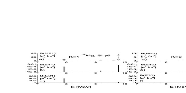
Figure 6: $B(M2K,\;0^{+}0_{\rm gs}\to 2^{-}K)$, $B(E1K,\;0^{+}0_{\rm gs}\to 1^{-}K)$, and $B(E3K,\;0^{+}0_{\rm gs}\to 3^{-}K)$ values for K=1 (left) and K=0 (right) in ²⁴Mg. In the plots (a) and (d), the total (filled triangles) and orbital (empty reverse triangles) $B(M2K)$ values are shown.

For a better understanding of these results, we provide in Table I more details on the structure of dipole states discussed above. Besides, the structure of K=0 state at 9.93 MeV is added since this state has a large $B(M2)$ value to be discussed in the next subsection. Table I shows that K=1 states at 7.92 and 9.79 MeV are dominated by two (proton and neutron) 2qp components of almost the same weight. The toroidal response depends on the relative sign of $X^{\nu}_{ii^{\prime}}$ in nn- and pp-components. In the 7.92-MeV state, the proton and neutron $X^{\nu}_{ii^{\prime}}$ have the same sign. As a result, proton and neutron toroidal flows in Fig. 2 are in phase and we get for this state a large T=0 toroidal strength, see Fig. 1 (a). Instead, in the 9.79-MeV state, the proton and neutron amplitudes $X^{\nu}_{ii^{\prime}}$ have opposite signs. This makes the proton and neutron toroidal flows in Fig. 5 (a)-(b) also opposite. The obtained destructive interference leads to the suppression of T=0 toroidal strength in this state. Further, the different signs of the proton and neutron $X^{\nu}_{ii^{\prime}}$ in the 9.79-MeV state result in a significant enhancement of the magnetization current (due to the constructive cooperation of the proton and neutron g-factors). For this reason, inclusion of ${\mathbb{j}}_{\rm m}$ leads a large increase of the total toroidal vortical strength in this state, see Fig. 4 (a). Furthermore, since absolute values of the proton $X^{\nu}_{ii^{\prime}}$ in 7.92-MeV and 9.79-MeV states are similar, the convective toroidal responses for these states, shown in Fig. 4 (a), are also comparable.

Note that the dominant 2qp components in Table I do not have spin-flip and so favor the orbital vortical flow. Altogether, the above analysis confirms the previous conclusions Ne_PRL18 ; RW87 ; Ne_Dres that toroidal flow in nuclei is mainly determined by the interplay of major 2qp components.

III.2 Electromagnetic transitions

For our aims, it is instructive to consider electromagnetic transitions from the ground state to the rotational bands built on the toroidal and compressional band heads. Below we inspect electric dipole $B(E1K,\;0^{+}0_{\rm gs}\to 1^{-}K)$, electric octupole $B(E3K,\;0^{+}0_{\rm gs}\to 3^{-}K)$, and magnetic quadrupole $B(M2K,\;0^{+}0_{\rm gs}\to 2^{-}K)$ reduced transition probabilities with $K=0,1$.

As mentioned in the Introduction, the $B(M2K)$ value can be used as an additional fingerprint of vortical toroidal states. Indeed, the vortical scissors sciss and twist twist modes are characterized by enhanced orbital M1 and M2 transitions, respectively. Further, the experimental techniques to extract M1 and M2 transition strengths in various reactions are now available, see e.g. determination of M2 strength from $(e,e^{\prime})$ reaction PVNC99 . Last but not least, the identification of mixed states by weak E2 and large orbital M1 transitions Pie08 shows that comparison of electric and magnetic transitions is a useful identification tool. Then it is worth to employ electromagnetic transitions for characterization of TS.

Table 2: The calculated reduced transition probabilities $B(M2K,0^{+}0_{\rm gs}\to 2^{-}K)$, $B(E1K,0^{+}0_{\rm gs}\to 1^{-}K)$, and $B(E3K,0^{+}0_{\rm gs}\to 3^{-}K)$ for low-energy $\nu$-states considered in Table I. For $B(M2K)$, the total, spin, and orbital values are given. The Weisskopf units BMv1 for ²⁴Mg are used: $B(M2)_{W.u}=$ 13.74 $\mu_{N}^{2}{\rm fm}^{2}$, $B(E1)_{W.u}=$ 0.537 $e^{2}{\rm fm}^{2}$, $B(E3)_{W.u}=$ 34.23 $e^{2}{\rm fm}^{6}$.

E	K	$B(M2)_{\rm tot}$	$B(M2)_{\rm spin}$	$B(M2)_{\rm orb}$	$B(E1)$	$B(E3)$
MeV		W.u.	W.u	W.u.	W.u.	W.u.
7.92	1	0.70	0.01	0.52	3.2 $\cdot 10^{-4}$	12
9.56	0	-	-	-	2.4 $\cdot 10^{-5}$	19
9.79	1	2.34	0.49	0.62	4.2 $\cdot 10^{-3}$	1.7
9.93	0	0.93	0.01	0.75	-	-

The reduced transition probabilities $B(M2K)$, $B(E1K)$, and $B(E3K)$ in ²⁴Mg are shown in Fig. 6. In panels (a) and (d), the total and orbital ($g^{q}_{s}=0$) $B(M2K)$ strengths are compared. It is easy to see that there is a remarkable correspondence between total/orbital $B(M21)$ in Fig. 6 (a) and total/orbital toroidal $B(E11)$ in Fig. 4 (a). This proves that $2^{-}1$ states based on the toroidal K=1 band heads exhibit large orbital $B(M21)$, i.e. there is a clear correlation between toroidal E11 and orbital M21 strengths. So, for low-energy dipole states, an enhanced orbital $B(M21)$ values can be used as an indicator for the toroidal mode.

Further, Table II shows that, in 7.92-MeV and 9.79-MeV states, orbital $B(M21)$ strengths reach 0.52 and 0.62 W.u., i.e. are rather large. In both states, the orbital strength dominates over the spin one, especially in 7.92-MeV state. Instead, the E11 strength in these states is $\sim 10^{-3}-10^{-4}$ W.u., i.e. very weak. This situation is similar to that for mixed-symmetry states with its enhanced M1 and weaken E2 transitions Pie08 (with the difference that mixed-symmetry states are mainly isovector while the low-energy toroidal states are basically isoscalar).

It is also interesting that the lowest toroidal 7.92-MeV state demonstrates a strong collective $0^{+}0\to 3^{-}1$ transition with $B(E31)$ = 12 W.u.. This means that, though 7.92-MeV state is mainly vortical, it also has some irrotational octupole component. Appearance of this component is explained by the large axial quadrupole deformation in ²⁴Mg, which leads to the strong mixing of the dipole and octupole modes. In the 7.92-MeV state, the octupole irrotational fraction seems to dominate over the dipole irrotational one. Note also that 2qp configurations $211\uparrow-330\uparrow$ dominating in 7.92-MeV and 9.79-MeV states (see Table I) fulfill the asymptotic selection rules for E31 and M21 transitions BM59 ; Sol (E31: $\Delta N=\pm 1,\pm 3$, $\Delta n_{z}=0,\pm 2$, $\Delta\Lambda=1$; M21: $\Delta N=\pm 1,\pm 3$, $\Delta n_{z}=0,\pm 1,\pm 2$, $\Delta\Lambda=0,1$), and not for E11 ($\Delta N=\pm 1$, $\Delta n_{z}=\pm 0$, $\Delta\Lambda=0$). This favors E31 and M21 transitions but hinders E11 ones. In 9.79-MeV state, $B(E31)$ is small because of the mutual compensation of proton and neutron contributions. In 7.92-MeV state, the hindered $B(E11)=10^{-3}-10^{-4}$ W.u. is nevertheless essentially larger than the experimental value 3.3 $10^{-6}$ W.u. NDS24Mg . So perhaps the irrotational dipole component in this state is weaker than in our calculations.

The left part of Fig. 4 shows transition probabilities for K=0 states. The 9.56-MeV state has hindered E10 and enhanced E30 strengths (see also Table II). In this state, the signature $\gamma$ coincides with the parity ($\gamma=\pi$ = - 1), its rotational band is $I^{\pi}=1^{-},3^{-},...$, and so the magnetic decay to the ground state is absent. Instead we have a noticeable amount of $B(M20,0^{+}0_{\rm gs}\to 2^{-}0)$ strength (together with vanishing $B(E10)$ and $B(E30)$) for the higher state at 9.93 MeV with $\gamma=-\pi$ = + 1. This state is not toroidal and so out of our interest. At the same time, this example shows that non-toroidal states can also have significant $B(M2)$. Thus, a large $B(M2)$ may be used for discrimination of the toroidal mode only in low-energy states with K=1.

The experimental data for low-energy spectra in ²⁴Mg NDS24Mg show $1^{-}$ levels at 7.555 and 8.437 MeV. Both levels can be reasonable candidates for toroidal excitations Ne_PRL18 . Moreover, the direct decay (most probably M2) from the first $I^{\pi}=2^{-}$ state at 8.864 MeV to the ground state is observed NDS24Mg . The decay is weak as compared with other decay channels of this state. Our QRPA approach is not enough to describe the complicated decay scheme in ²⁴Mg. Nevertheless it allows to state that orbital M21 transitions from low-energy K=1 states can serve as promising indicators of the toroidal mode in deformed nuclei.

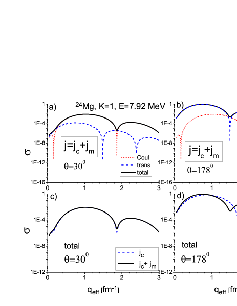
Figure 7: The $(e,e^{\prime})$ cross-section for $I^{\pi}K=1^{-}1$ state at 7.92 MeV, calculated for the scattering angles $\theta=30^{\circ}$ (left) and $178^{\circ}$ (right). In the upper plots (a)-(b), the Coulomb, transversal and total cross-sections are compared. In the bottom plots (c)-(d), the total cross-sections with and without ${\mathbb{j}}_{\rm m}$ are shown.

III.3 $(e,e^{\prime})$ reaction

To discriminate TS from other dipole modes, we need a reaction sensitive to the nuclear interior. The inelastic electron scattering $(e,e^{\prime})$ is just the proper case. In the Plane Wave Born Approximation (PWBA), the $(e,e^{\prime})$ cross-section for $E(M)\lambda$ excitations reads HB83

$$\frac{d\sigma}{d\Omega}(\theta,q,E_{i})=4\pi\sigma_{\rm Mott}(\theta,E_{i})f_{\rm rec}(\theta,E_{i})$$

$$\cdot \left[[F^{C}_{E\lambda}(q)]^{2}+\left(\frac{1}{2}+\tan^{2}(\frac{\theta}{2})\right)\left([F^{T}_{M\lambda}(q)]^{2}+[F^{T}_{E\lambda}(q)]^{2}\right)\right]$$

where $\sigma_{\rm Mott}(\theta,E_{i})$ is the Mott cross section for the unit charge, $f_{\rm rec}(\theta,E_{i})$ is the recoil factor, $E_{i}$ is the incident electron energy, $\theta$ is the scattering angle. Further, $F^{C}_{E\lambda}(q)$, $F^{T}_{E\lambda}(q)$, and $F^{T}_{M\lambda}(q)$ are Coulomb and transversal electric and magnetic form factors as a function of the momentum transfer $q$. Here, $q=(2/(\hbar c)\sqrt{E_{i}E_{f}}\sin(\theta/2)$ where $E_{f}=E_{i}-E_{\nu}$ is the final electron energy and $E_{\nu}$ is the nuclear excitation energy. For the light nucleus ²⁴Mg, the Coulomb distortions should be small and so PWBA is the relevant approximation. We also can use $f_{\rm rec}(\theta,E_{i})$=1. To take roughly into account the Coulomb distortions, the figures below are plotted as a function of the effective momentum transfer

$$q_{\rm eff}=q(1+1.5\frac{Z\alpha\hbar c}{E_{i}R})$$ (11)

where $Z$ is the nuclear charge and $R=1.12A^{1/3}$ fm.

First of all, let’s consider the $(e,e^{\prime})$ cross section for the toroidal states and inspect the effect of the magnetization current ${\mathbb{j}}_{\rm m}$ on them. Since the toroidal mode is transversal Bas93 ; Mis06 ; Dub75 , it is natural to look for its signature in the dipole transversal electric form factor $F^{T}_{E1}$ at backward scattering angles.

In Fig. 7, the normalized cross-section $\sigma=\frac{d\sigma}{d\Omega}/\sigma_{\rm Mott}$ for the 7.92-MeV state in ²⁴Mg is plotted for small $\theta$ = 30^∘ and large $\theta$ = 178^∘ scattering angles. Panels (a)-(b) show that, as expected, the total cross-section is dominated by the Coulomb part at $\theta$ = 30^∘ and by electric transversal part at $\theta$ = 178^∘. Further, panels (c)-(d) show that inclusion of $j_{\rm m}$ does not almost influence the cross-section at $\theta$ = 30^∘ but leads to considerable changes for $q_{\rm eff}>1$ fm^-1 at the backward angle $\theta=178^{\circ}$. The latter significantly complicates the direct search of TS in the transversal cross-section at large $\theta$.

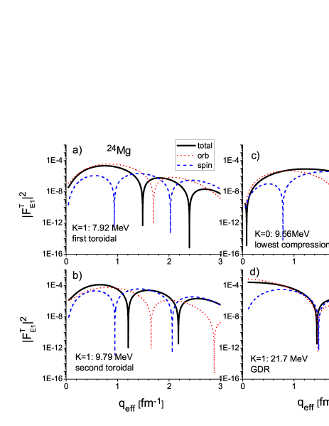
Figure 8: Squared electric transversal form factors $|F^{T}_{E1}|^{2}$ calculated with the total (black solid line), orbital (red dotted line) and spin (dash blue line) nuclear current for different QRPA states: toroidal $I^{\pi}K=1^{-}1$ at 7.92 MeV (a) and 9.79 MeV (b), compressional $1^{-}0$ at 9.56 MeV (c), and GDR $1^{-}1$ at 21.7 MeV (d).

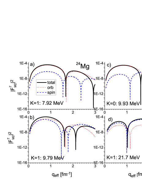
Figure 9: Squared magnetic transversal form factors $|F^{T}_{M2}|^{2}$ calculated with the total (black solid line), orbital (red dotted line) and spin (dash blue line) nuclear current for different QRPA states: toroidal $I^{\pi}K=1^{-}1$ at 7.92 MeV (a) and 9.79 MeV (b), compressional $1^{-}0$ at 9.93 MeV (c), and GDR $1^{-}1$ at 21.7 MeV (d).

We see that the Coulomb cross-section for the toroidal 7.92-MeV state has a distinctive minimum at $q_{\rm eff}<0.2\;\rm{fm}^{-1}$. Similar minima were earlier found for low-energy dipole states in light N=Z spherical doubly magic nuclei like ¹⁶O, see Mi75 for experiment and Ca90 ; Papa11 ; Ne_20Ne for discussion. Following Papa11 , these states can also exhibit toroidal flow. Most probably, however, these minima are caused not by toroidal flow but rather by destructive competition between the dominant T=0 and minor T=1 components in these states Ca90 ; Papa11 .

Nevertheless the toroidal mode leaves in $(e,e^{\prime})$ scattering some signatures suitable for its discrimination. These signatures are illustrated in Fig. 8 where the squared transversal form factors $|F^{T}_{E1}|^{2}$ for different dipole states in ²⁴Mg are plotted. Here we consider the toroidal K=1 states at 7.92 and 9.79 MeV, the compressional K=0 state at 9.56 MeV and the high-energy K=1 state at 21.7 MeV from the isovector giant dipole resonance (GDR). The form factors are calculated with the total ${\mathbb{j}}_{\rm c}+{\mathbb{j}}_{\rm m}$, convective (orbital) ${\mathbb{j}}_{\rm c}$, and spin ${\mathbb{j}}_{\rm m}$ nuclear currents.

Fig. 8 shows that total form factors for toroidal 7.92-MeV and 9.79-MeV states (plots (a)-(b)) are more structured as they have two diffraction minima at $q_{\rm eff}<3\;{\rm fm}^{-1}$) and, in this sense, significantly deviate from the form factors for other states (plots (c)-(d)). In the orbital form factors, the diffraction minima lie essentially higher than in the spin ones. For toroidal states, just destructive interference of the orbital and spin contributions gives diffraction minima in the total $|F^{T}_{E1}|^{2}$. They are at $q^{\rm min}_{\rm eff}=1.50,2.39\;\rm{fm}^{-1}$ in 7.92-MeV state and at $q^{\rm min}_{\rm eff}=1.20,2.17\;\rm{fm}^{-1}$ in 9.79-MeV state. Neither orbital, nor spin contribution alone can describe the behavior of the total $|F^{T}_{E1}|^{2}$. Therefore this behavior can be used as a sensitive tool for determination of the orbital/spin interplay. One may state that the QRPA $\nu$-th wave function correctly describes the orbital and spin contributions only if it reproduces the features of the total $|F^{T}_{E1}|^{2}$ at large scattering angles.

Note also that, following panels (a)-(b), the orbital (toroidal) contribution dominates over the spin one at $q_{\rm eff}<1.1\;\rm{fm}^{-1}$. The dominance is impressive for 7.92-MeV state.

Further, Fig. 9 shows the squared magnetic form factors $|F^{T}_{M2}|^{2}$ calculated with the total ${\mathbb{j}}_{\rm c}+{\mathbb{j}}_{\rm m}$, convective (orbital) ${\mathbb{j}}_{\rm c}$, and spin ${\mathbb{j}}_{\rm m}$ nuclear currents. In the plots (a), (b), and (d), excitations $I^{\pi}K=2^{-}1$ related to the states in Fig. 8 are considered. In the plot (c), we consider the compressional K=0 9.93-MeV state with the signature $\gamma=-\pi$ = + 1 and non-zero $B(M20,0^{+}0_{\rm gs}\to 2^{-}0)$ value (see Table II). Fig. 9 (a) shows that, in the toroidal K=1 7.92-MeV state, the orbital contribution strongly dominates at $q_{\rm eff}<1.6\;\rm{fm}^{-1}$. The same takes place in Fig. 9 (c) for K=0 9.93-MeV state. In both cases, the first diffraction minimum is fully determined by the orbital form factor. In the toroidal K=1 9.79-MeV state, the dominance of the orbital part is weaker but we have the specific second diffraction minimum at $q^{\rm min}_{\rm eff}=2.12\;\rm{fm}^{-1}$, produced by the destructive interference of the orbital and spin parts. For both toroidal 7.92-MeV and 9.79-MeV states, the formfactors $|F^{T}_{M2}|^{2}$ are structured enough to probe the wave functions of these states and judge on the important (or even dominant) role of the orbital flow.

Altogether one may propose the following two-step scheme for discrimination of individual vortical toroidal states in $(e,e^{\prime})$ reaction.

1) The calculations (e.g. QRPA) should identify the relevant candidates for the toroidal dipole states. They should be low-energy K=1 states with the following properties: i) large toroidal strength like in Figs. 1 and 4, ii) typical toroidal picture for the convective current density, like in Figs. 2 and 5, iii) enhanced $B(M2)$ and weak $B(E1)$ transition rates for decays to the ground state.

2) The wave functions of the chosen states should reproduce the main features of the total squared transversal form factors $|F^{T}_{E1}|^{2}$ and $|F^{T}_{M2}|^{2}$ at back scattering angles. In particular, magnitudes of form factors at diffraction maxima and positions of diffraction minima should be described. As shown in our study, the behavior of these form-factors is very sensitive to the interference of the spin and orbital contributions. If the experimental $(e,e^{\prime})$ data are not reproduced by the spin contribution alone but reasonably described by the total spin + orbital contribution, then: i) wave functions of the chosen states can be assumed as reliable and ii) toroidal distributions of their convective currents can be considered as realistic.

To check this two-step scheme, the new $(e,e^{\prime})$ experiments for ²⁴Mg are desirable. For this aim, the electron beams with the incident electron energy 40-90 MeV, available e.g. in Darmstadt facilities PVNC99 ; Ri04 , could be used.

Note that a similar prescription was earlier employed for confirmation of the vortical twist M2 mode in Darmstadt $(e,e^{\prime})$ experiment PVNC99 . Namely, the orbital M2 contribution to the backward electron scattering was justified by comparison of the calculated spin and spin+orbital M2 form factors with experimental data. The fact that only spin + orbital contribution (but not spin contribution alone) was sufficient to describe the experimental data, was claimed as a robust signal of a strong orbital twist M2 flow.

Note that our QRPA calculations do not take into account such factors as the nuclear triaxiality and coupling with complex configurations (CCC). By our opinion, these factors should not essentially change our main results. Indeed, following various calculations Rod10 ; Be08 ; Yao11 ; Hino11 ; Kimura12 , ²⁴Mg has a weak triaxial softness in the ground state and more triaxiality in positive-parity excited states. In the lowest negative-parity dipole states, the triaxiality is found negligible in K=1 and significant in K=0 excitations Kimura12 . Since we mainly address low-energy K=1 excitations with the dominant large-magnitude axial prolate deformation, the treatment of ²⁴Mg as an axial prolate nucleus should be reasonable. Besides, the dipole K=1 states of our interest have a low collectivity and so should exhibit a minor CCC impact.

IV Conclusions

A possibility to search individual E1 toroidal states (TS) in inelastic electron scattering $(e,e^{\prime})$ to back angles was scrutinized within the self-consistent quasiparticle random-phase-approximation (QRPA) model using the Skyrme force SLy6. As a relevant example, the low-energy dipole states with K=0 and 1 in axially deformed ²⁴Mg were thoroughly explored. We inspected vortical toroidal and irrotational compressional E1 responses, transition rates $B(E1,0^{+}0_{\rm gs}\to 1^{-}K),\;B(E3,0^{+}0_{\rm gs}\to 3^{-}K)$ and $B(M2,0^{+}0_{\rm gs}\to 2^{-}K)$, distributions of transition currents, form factors and cross sections for $(e,e^{\prime})$ reaction. The cross sections were calculated in the Plane Wave Born Approximation. In the relevant cases, the separate contributions of the convection ${\mathbb{j}}_{\rm c}$, and magnetization ${\mathbb{j}}_{\rm m}$ parts of nuclear current were analyzed.

The analysis of these results led to a two-step scheme for the search of toroidal K=1 states in $(e,e^{\prime})$ scattering. In the first step, QRPA calculation are used to determine the promising candidates for toroidal states (with large toroidal responses, distinctive toroidal distribution of the convective nuclear current and significant $B(M2)$ values). In the second step, these states are checked to reproduce the pattern of the experimental data for E1 and M2 transversal form factors in $(e,e^{\prime})$ scattering to back angles. Following our analysis, these form factors exhibit a strong interference of the convective (orbital) and magnetization (spin) contributions of the nuclear current and this interference determines, in a large extent, the features (form factor maxima, positions of the first two diffraction minima, etc) of the form factors. As a result, E1 and M2 transversal form factors can serve as sensitive probes for the interplay between orbital and spin contributions. If only the combined spin+orbital contributions (but not spin alone) allow to reproduce the experimental behavior of these form factors, then one may claim that i) the structure of the chosen calculated state correctly matches the orbital and spin fractions and ii) the toroidal distribution of the nuclear current in this state is indeed realistic. A similar prescription was earlier used in the experimental search of the vortical twist M2 mode in $(e,e^{\prime})$ reaction PVNC99 . Note that involvement of $B(M2)$ values and M2 form factors for discrimination of E1 toroidal states is relevant only for deformed nuclei and this part of the analysis should be skipped in spherical nuclei.

In the proposed identification scheme, the interference between the orbit and spin contributions to the experimentally accessible $(e,e^{\prime})$ form factors is the key element. The toroidal strengths and current distributions as such can hardly be measured directly, but can be used as pre-selectors to choose from QRPA calculations the proper candidate states for the further analysis of $(e,e^{\prime})$ scattering.

In the present study for ²⁴Mg, two individual toroidal K=1 states at 7.92 and 9.97 MeV were found and thoroughly explored. It was shown that the magnetization current ${\mathbb{j}}_{\rm m}$ has a strong impact for these states. Just this considerable magnetic contribution together with the dominant orbital contribution leads to the significant interference effects in E1 and M2 form factors and so paves the way for discrimination of the toroidal states. Furthermore, we have found that ${\mathbb{j}}_{\rm m}$ can produce itself the magnetization toroidal states.

The above scheme can be also used for heavier nuclei where we deal not with individual toroidal states but rather with broadly spread toroidal strength functions. In this case, we should work with the averaged characteristics using the technique described in Ref. Rep13 for ²⁰⁸Pb.

In principle, similar schemes can be applied to other reactions ($(e,e^{\prime}\gamma)$, $\alpha,\alpha^{\prime})$, $(p,p^{\prime})$, etc) relevant for the search of toroidal dipole states (see Ref. Bracco19 for the recent review of various reactions for dipole excitations). By our opinion, there is no problem to excite TS in nuclei. Following our present analysis for ²⁴Mg and previous analysis for a variety of medium and heavy nuclei Kv11 ; Rep17 ; RNKR_EPJA , even basically vortical dipole states usually have a minor irrotational fraction RNKR_EPJA and this fraction can be used as a doorway for excitation of the toroidal mode in various reactions. The main trouble is not to excite vortical TS but to identify them. This is a part of a general fundamental problem of identification of vorticity in nuclei. The problem is indeed demanding since its solution requires a theory-assisted analysis combining information on nuclear structure and reaction mechanisms. Hopefully, the search of the vortical toroidal mode in $(e,e^{\prime})$ reaction will be an important and encouraging step in this direction.

References

- (1) V.O. Nesterenko, A. Repko, J. Kvasil, and P.-G. Reinhard, Phys. Rev. Lett. 120, 182501 (2018).
- (2) V.O. Nesterenko, J. Kvasil, A. Repko, and P.-G. Reinhard, Eur. Phys. J. Web of Conf. 194, 03005 (2018).
- (3) Yoshiko Kanada-En’yo and Yuki Shikata, Phys. Rev. C 95, 064319 (2017).
- (4) Yuki Shikata, Yoshiko Kanada-En’yo, and Horiyuki Morita, Prog. Theor. Exp. Phys. 063D01 (2019).
- (5) Yoshiko Kanada-En’yo, Yuki Shikata, and Horiyuki Morita, Phys. Rev. C 97, 014303 (2018).
- (6) Yoshiko Kanada-En’yo and Yuki Shikata, Phys. Rev. C 100, 014301 (2019).
- (7) Yoshiko Kanada-En’yo and Hisashi Horiuchi, Front. Phys. 13, 132108 (2018).
- (8) S. F. Semenko, Sov. J. Nucl. Phys. 34, 356 (1981).
- (9) S. I. Bastrukov, Ş. Mişicu, and A. V. Sushkov, Nucl. Phys. A 562, 191 (1993).
- (10) Ş. Mişicu, Phys. Rev. C 73, 024301 (2006).
- (11) E.B. Balbutsev, I.V. Molodtsova, and A.V. Unzhakova, Europhys. Lett. 26, 499 (1994).
- (12) N. Ryezayeva, T. Hartmann, Y. Kalmykov, H. Lenske, P. von Neumann-Cosel, V.Yu. Ponomarev, A. Richter, A. Shevchenko, S. Volz, and J. Wambach, Phys. Rev. Lett. 89, 272502 (2002).
- (13) G. Colo, N. Van Giai, P.F. Bortignon, and M.R. Quaglia, Phys. Lett. B 485, 362 (2000).
- (14) D. Vretenar, N. Paar, P. Ring, and T. Nikšić, Phys. Rev. C 65, 021301(R) (2002).
- (15) N. Paar, D. Vretenar, E. Khan, and G. Colo, Rep. Prog. Phys. 70, 691 (2007).
- (16) J. Kvasil, V. O. Nesterenko, W. Kleinig, P.-G. Reinhard, and P. Vesely, Phys. Rev. C 84, 034303 (2011).
- (17) A. Repko, P.-G. Reinhard, V. O. Nesterenko, and J. Kvasil, Phys. Rev. C 87, 024305 (2013).
- (18) P.-G. Reinhard, V. O. Nesterenko, A. Repko, and J. Kvasil, Phys. Rev. C 89, 024321 (2014).
- (19) V.O. Nesterenko, J. Kvasil, A. Repko, W. Kleinig, and P.-G. Reinhard, Phys. Atom. Nucl. 79, 842 (2016).
- (20) A. Repko, J. Kvasil, V. O. Nesterenko, and P.-G. Reinhard, Eur. Phys. J. A 53, 221 (2017).
- (21) D. H. Youngblood, Y.-W. Lui, B. John, Y. Tokimoto, H. L. Clark, and X. Chen, Phys. Rev. C 69, 054312 (2004).
- (22) M. Uchida, H. Sakaguchi, M. Itoh, M. Yosoi, T. Kawabata, Y. Yasuda, H. Takeda, T. Murakami, S. Terashima, S. Kishi, U. Garg, P. Boutachkov, M. Hedden, B. Kharraja, M. Koss, B. K. Nayak, S. Zhu, M. Fujiwara, H. Fujimura, H. P. Yoshida, K. Hara, H. Akimune, and M. N. Harakeh, Phys. Rev. C 69, 051301(R) (2004).
- (23) N. Lo Iudice and F. Palumbo, Phys. Rev. Lett. 41, 1532 (1978).
- (24) G. Holzward and G. Ekardt, Z. Phys. A 283, 1532 (1978).
- (25) M. Bender, P.-H. Heenen, and P.-G. Reinhard, Rev. Mod. Phys. 75, 121 (2003).
- (26) E. Chabanat, P. Bonche, P. Haensel, J. Meyer, and R. Schaeffer, Nucl. Phys. A635, 231 (1998).
- (27) A. Repko, J. Kvasil, V. O. Nesterenko, and P.-G. Reinhard, arXiv:1510.01248[nucl-th].
- (28) P. Ring and P. Schuck, The Nuclear Many-Body Problem (Springer-Verlag, Berlin, 1980).
- (29) V.O. Nesterenko, W. Kleinig, J. Kvasil, P. Vesely, and P.-G. Reinhard, Int. J. Mod. Phys. E 17, 89 (2008).
- (30) M. N. Harakeh and A. van der Woude, Giant Resonances (Clarendon Press, Oxford, 2001).
- (31) N. Van Giai and H. Sagawa, Nucl. Phys. A 371, 1 (1981).
- (32) A. Repko, J. Kvasil, and V.O. Nesterenko, Phys. Rev. C 99, 044307 (2019).
- (33) K. Yoshida and N.V. Giai, Phys. Rev. C 78, 064316 (2008).
- (34) A. Bohr and B.R. Mottelson, Nuclear Structure Vol. 1 (Benjamin, New York, 1969).
- (35) A. Repko and J. Kvasil, Acta Phys. Polon. B Proceed. Suppl. 12, 689 (2019); arXiv:1904.11259 [nucl-th].
- (36) D.G. Raventhall and J. Wambach, Nucl. Phys. A 475, 468 (1987).
- (37) V.O. Nesterenko, A. Repko, P.-G. Reinhard, and J. Kvasil, EPJ Web of Conferences, 93, 01020 (2015).
- (38) P. von Neumann-Cosel, F. Neumeyer, S. Nishizaki, V.Yu. Ponomarev, C. Rangacharyulu, B. Reitz, A. Richter, G. Schrieder, D.I. Sober, T. Waindzoch, and J. Wambach, Phys. Rev. Lett. 82, 1105 (1999).
- (39) N. Pietrallaa, P. von Brentano, A.F. Lisetskiy, Prog. Part. Nucl. Phys. 60, 225 (2008).
- (40) B. Mottelson and S.G. Nilsson, Mat. Fys. Skr. Dan. Vid. Selsk. 1, n. 8 (1959).
- (41) V.G. Soloviev, Theory of Complex Nuclei (Pergamon Press, Oxford, 1976).
- (42) R.B. Firestone, Nucl. Data Sheets, 108, 2319 (2007).
- (43) J. Heisenberg and H.P. Blok, Ann. Rev. Nucl. Part. Sci. 33, 569 (1983).
- (44) V.M. Dubovik and A.A. Cheshkov, Sov. J. Part. Nucl. 5, 318 (1975).
- (45) H. Miska, H.D. Gräf, A. Richter, D. Schüll, E. Spamer and O. Titze, Phys. Lett. B 59, 441 (1975).
- (46) B. Castel, Y. Okuhara, and H. Sagawa, Phys. Rev. C 42, R1203 (1990).
- (47) P. Papakonstantinou, V.Yu. Ponomarev, R. Roth, and J. Wambach, Eur. Phys. J. A 47, 14 (2011).
- (48) A. Repko, V.O. Nesterenko, J. Kvasil, and P.-G. Reinhard, arXiv:1903.01348[nucl-th], to be published in Eur. Phys. J. A.
- (49) A. Richter, Nucl. Phys. A 731, 59 (2004).
- (50) T.R. Rodriguez and J.L. Egido, Phys. Rev. C 81, 064323 (2010).
- (51) M. Bender and P.-H. Heenen, Phys. Rev. C 78, 024309 (2008).
- (52) J.M. Yao, H. Mei, H. Chen, J. Meng, P. Ring, and D. Vretenar, Phys. Rev. C 83, 014308 (2011).
- (53) N. Hinohara and Y. Kanada-En’yo, Phys. Rev. C 83, 014321 (2011).
- (54) M. Kimura, R. Yoshida, and M. Isaka, Prog. Theor. Phys. 127, 287 (2012).
- (55) A. Bracco, E.G. Lanza, and A. Tamii, Prog. Part. Nucl. Phys. 106, 360 (2019).