We show that the general method of Lie algebra expansions can be applied to re-construct several algebras and related actions for non-relativistic gravity that have occurred in the recent literature. We explain the method and illustrate its applications by giving several explicit examples. The method can be generalized to include the construction of actions for ultra-relativistic gravity, i.e. Carroll gravity, and non-relativistic supergravity as well.

1 Introduction

During the last few years, there has been a renewed interest in non-relativistic gravity due to its possible role in holography where gravity is used as a tool to probe the dark corners of quantum field theories or in effective field theory where gravitational fields are used as geometrical background response functions [3, 4].

It turns out that, in contrast to general relativity, there are many different versions of non-relativistic gravity theories. They are all invariant under reparametrizations but differ in the fact that they are invariant under distinct extensions of the Galilei symmetries. The simplest example is the so-called Galilei gravity theory which is invariant under the un-extended Galilei symmetries [5]. Instead, Newtonian gravity and its frame-independent reformulation, called Newton-Cartan (NC) gravity, is invariant under the symmetries corresponding to a central extension of the Galilei algebra, called the Bargmann algebra. In three dimensions there even exists a non-relativistic gravity theory that is based on a Galilei algebra with two central extensions [6, 7, 8] while recently, in four dimensions, an interesting example of a non-relativistic gravity theory based upon an even larger extension of the Bargmann algebra containing non-central generators has been encountered [9].

It is well known that the generator of time translations of the Galilei algebra plays a different role than the generators of space translations. This is related to the fact that absolute time plays a special role in Newtonian gravity. However, it turns out that this type of Galilei algebra is only suitable when coupling non-relativistic gravity to particles. Instead, when coupling to extended objects with $p$ spatial extensions, i.e. $p$-branes, one needs to foliate spacetime in a different way, according to the number of longitudinal and transverse directions (directions parallel to the $p$-brane’s worldvolume and the rest). This leads to a different kind of Galilei algebra where, for a given spacetime of dimension $D$, the translation generators of the Galilei algebra are given by the following set of generators

$$(H_{A},P_{a})\,,\hskip 28.45274ptA=0,1,\cdots,p;\qquad a=p+1,\cdots,D-1\,,$$ (1.1)

which correspond to translations along longitudinal and transverse directions, respectively. We will denote these different kinds of Galilei algebra as $(D,p)$ Galilei algebras. The related non-relativistic gravity theories will be called $(D,p)$ Galilei gravity. Like in the particle case, there are further non-relativistic gravity theories that are based upon extensions of the $(D,p)$ Galilei algebras. A recent example is string NC gravity [10] that is based upon a $p=1$ (string) version of the Bargmann algebra [11].

It is a relatively simple matter to construct an action for $(D,p)$ Galilei gravity. One simply takes an appropriate non-relativistic limit of the first-order Einstein-Hilbert action, thereby generalizing the case of Galilei gravity discussed in [5]. It is much harder to construct an action for NC gravity that is based on the Bargmann algebra. Taking the non-relativistic limit of general relativity without obtaining fatal divergencies can only be done at the level of the equations of motion. Similarly, performing a null-reduction of five-dimensional general relativity does not lead to an action for 4-dimensional NC gravity but only to its equations of motion [14]. Despite these difficulties, several actions for non-relativistic gravity, based on extensions of the Galilei algebra, have been constructed in the recent literature. One example we already mentioned is the three-dimensional action of [6, 7, 8], which is based upon a three-dimensional Galilei algebra with two central central extensions. More recent examples are the 4D non-relativistic gravity action of [9], the 4D extended string Newton-Cartan gravity action of [15] and the 3D action of [16]. 

The purpose of this paper is to show that all algebras underlying the above actions can be obtained via the Lie algebra expansion of the relativistic Poincaré algebra. The Lie algebra expansion method was first used in [17] and later studied from a more general perspective and applied to 3D Chern Simons supergravity and the M-theory superalgebra in [18, 19]. The Lie algebra expansion method is a general method that in the present case allows one to obtain from the relativistic Poincaré algebra a number of extensions of the non-relativistic $(D,p)$ Galilei algebra containing extra generators some of which can be central extensions. The first algebra in the expansion is always the un-extended Galilei algebra which has the additional feature that it can be obtained as a Inönü-Wigner contraction of the Poincaré algebra. The other algebras are obtained as consistent truncations of the full expansion.

This method can also be used to obtain actions for the non-relativistic gravity theories associated to the finite extended-Galilei algebras obtained as truncations. In most cases, but, unfortunately, not always, it produces an invariant action. In particular, it gives an invariant action for the $(D,p)$ Galilei algebras, for any $D$ and $p$. These actions can be obtained by taking a non-relativistic limit of the Einstein-Hilbert action that mimics the corresponding Inönü-Wigner contraction of the Poincaré algebra [5]. Recently, by applying the Lie algebra expansion directly at the level of the action, it has been observed that in three dimensions the first algebra that occurs in the expansion beyond the Galilei algebra, also allows an action [26]. In fact, it precisely leads to the action of [7, 8]. Even the supersymmetric action of [7] was derived in this way.

In this paper we are going to explain how the Lie algebra expansion procedure works, applying it to a few important examples. In particular, we will derive a rule that tells, for a given truncation and given values of $D$ and $p$, how many orders one needs to go in the expansion beyond the lowest-order (Galilei algebra) for an action to exist. For instance, in $D=4$ we will find that in the string case the first algebra beyond the string Galilei algebra leads to the action of [15] but that, in the particle case, one must take the second algebra in the expansion, which is precisely the algebra of [9].

The organization of this paper is as follows. In section 2 we will give a formal description of the Lie algebra expansion procedure. Next, in section 3, we will give explicit expressions for the Lie algebra expansion of the Poincaré algebra for general $D$ and $p$. In section 4, we will discuss a few subtleties that occur when constructing an invariant action. In particular, we will discuss the role of the so-called $P$-symmetries and we will give a rule that states for which truncations and which values of $D$ and $p$ an invariant action exist. In the next section, we will give five examples of actions for non-relativistic gravity thereby re-producing several results given in the literature. Finally, in the conclusions, we will discuss a relation between the Lie algebra expansion and taking non-relativistic limits. We will also mention how the Lie algebra expansion procedure can be applied to a variety of new situations. Finally, we have delegated the full proof of the rule that indicates when an invariant action exists to appendix A while in appendix B we give a few more details about the third example in the main text.

2 Lie algebra expansions

The Lie algebra expansion is a method that, starting from a given Lie algebra, leads to new Lie algebras. These algebras are, in general, of higher dimension than the original one. In this section we give a general description of the method.

Quite generally, the Lie algebra expansion of an algebra is obtained by formally expanding the Maurer-Cartan one-forms of the dual version of the algebra in a power series of a parameter $\lambda$, each coefficient being a new one-form. One next substitutes this expansion into the Maurer-Cartan equations of the algebra and identifies equal powers of $\lambda$. This results into an infinite set of Maurer-Cartan equations that can later be truncated consistently to obtain a number of finite-dimensional Lie algebras.

To be specific, we describe the method in the case that is relevant to us, that is, when the original algebra $\mathfrak{g}$ can be split, as a vector space, into the direct sum $\mathfrak{g}=V_{0}\oplus V_{1}$ of two subspaces $V_{0}$ and $V_{1}$ with

$$[V_{0},V_{0}]\subset V_{0}\ ,\quad[V_{0},V_{1}]\subset V_{1}\ ,\quad[V_{1},V_{1}]\subset V_{0}\,.$$ (2.1)

This means that $V_{0}$ and $V_{1}$ form a symmetric pair. Let $X_{i}$, $i=1\dots\textrm{dim}\mathfrak{g}$, be a set of generators of the starting Lie algebra $\mathfrak{g}$ whose commutation rules read

$$[X_{i},X_{j}]=C_{ij}{}^{k}X_{k}\,.$$ (2.2)

Let $X_{i}=\{X_{i_{0}},X_{i_{1}}\}$ with $X_{i_{0}}\in V_{0}$, $X_{i_{1}}\in V_{1}$, $i_{0}=1\dots\textrm{dim}V_{0}$, $i_{1}=1\dots\textrm{dim}V_{1}$. Then, the condition (2.1) implies that

$$C_{i_{0}j_{0}}{}^{k_{1}}=0\,,\hskip 28.45274ptC_{i_{0}j_{1}}{}^{k_{0}}=0\,,\hskip 28.45274ptC_{i_{1}j_{1}}{}^{k_{1}}=0\,.$$ (2.3)

We now consider the dual formulation in terms of the Maurer-Cartan one-forms $\omega^{i}=\{\omega^{i_{0}},\omega^{i_{1}}\}$. The commutators (2.2) are equivalent to the Maurer-Cartan equations

$$d\omega^{k}=-\frac{1}{2}C_{ij}{}^{k}\omega^{i}\wedge\omega^{j}\ .$$ (2.4)

The Jacobi identity in this formulation corresponds to $dd\equiv 0$. It is now consistent to expand the Maurer-Cartan one-forms as follows:

$$\omega^{i_{0}} =\sum_{\alpha_{0}=0,\,\alpha_{0}\,\,\textrm{even}}^{\infty}\accentset{(\alpha_{0})}{\omega}{}^{\,i_{0}}\lambda^{\alpha_{0}}\ ,$$ (2.5a)

$$\omega^{\,i_{1}} =\sum_{\alpha_{1}=1,\,\alpha_{1}\,\,\textrm{odd}}^{\infty}\accentset{(\alpha_{1})}{\omega}{}^{\,i_{1}}\lambda^{\alpha_{1}}\ ,$$ (2.5b)

where we have introduced new indices $(\alpha_{0})$ and $(\alpha_{1})$ on top of the Maurer-Cartan one-forms to indicate the order of the corresponding terms in the expansion. By inserting these expansions into the Maurer-Cartan equations (2.4) and identifying equal powers of $\lambda$, the following infinite set of Maurer-Cartan equations is obtained:

$$d\accentset{(\gamma_{s})}{\omega}{}^{\,k_{s}}=-\frac{1}{2}C_{i_{p},\alpha_{p}\,j_{q},\beta_{q}}{}^{k_{s},\gamma_{s}}\accentset{(\alpha_{p})}{\omega}{}^{\,i_{p}}\wedge\accentset{(\beta_{q})}{\omega}{}^{\,j_{q}}\ ,$$ (2.6)

where $s,p,q=0,1$ and

$$C_{i_{p},\alpha_{p}\,j_{q},\beta_{q}}{}^{k_{s},\gamma_{s}}=\left\{\begin{array}[]{ll}C_{i_{p}\,j_{q}}{}^{k_{s}}\,,&\,\,\,\,\hbox{$\gamma_{s}=\alpha_{p}+\beta_{q}$;}\\ &\\ 0\,,&\,\,\,\,\hbox{otherwise.}\\ \end{array}\right.$$ (2.7)

These equations are dual to an infinite set of commutators that satisfy the Jacobi identity.

To obtain finite-dimensional Lie algebras, we substitute the following finite expansions, for given integers $(N_{0},N_{1})$,

$$\omega^{i_{0}} =\sum_{\alpha_{0}=0,\,\alpha_{0}\,\,\textrm{even}}^{N_{0}}\accentset{(\alpha_{0})}{\omega}{}^{\,i_{0}}\lambda^{\alpha_{0}}\ ,$$ (2.8a)

$$\omega^{i_{1}} =\sum_{\alpha_{1}=1,\,\alpha_{1}\,\,\textrm{odd}}^{N_{1}}\accentset{(\alpha_{1})}{\omega}{}^{\,i_{1}}\lambda^{\alpha_{1}}\,,$$ (2.8b)

in such a way that the result is a consistent set of Maurer-Cartan equations. This is true if and only if one of the following conditions is satisfied [18]:

$$N_{0}=N_{1}+1\hskip 14.22636pt\,\,\,\,\text{or}\hskip 14.22636pt\,\,\,\,N_{1}=N_{0}+1\ .$$ (2.9)

We will denote the algebras corresponding to these two conditions as $\mathfrak{g}(N_{0},N_{1})=\mathfrak{g}(N+1,N)$ and $\mathfrak{g}(N_{0},N_{1})=\mathfrak{g}(N,N+1)$, respectively. Note that in the first case $N$ has to be odd, while in the second it has to be even

We may also consider the gauge fields $\accentset{(\alpha_{s})}{A}{}^{\,i_{s}}$ and curvatures $\accentset{(\alpha_{s})}{F}{}^{\,i_{s}}$ for the new Lie algebras. They are related by

$$\accentset{(\gamma_{s})}{F}{}^{\,\,\,k_{s}}=d\accentset{(\gamma_{s})}{A}{}^{\,\,k_{s}}+\frac{1}{2}C_{i_{p},\alpha_{p}\,j_{q},\beta_{q}}{}^{k_{s},\gamma_{s}}\accentset{(\alpha_{p})}{A}{}^{\,i_{p}}\wedge\accentset{(\beta_{q})}{A}{}^{\,j_{q}}$$ (2.10)

with $\gamma_{s}=\alpha_{p}+\beta_{q}$. The gauge fields transform as

$$\delta\accentset{(\gamma_{s})}{A}{}^{\,\,k_{s}}=d\accentset{(\gamma_{s})}{a}{}^{\,\,\,i_{s}}-C_{i_{p},\alpha_{p}\,j_{q},\beta_{q}}{}^{k_{s},\gamma_{s}}\,\,\accentset{(\alpha_{p})}{a}{}^{\,\,i_{p}}\accentset{(\beta_{q})}{A}{}^{\,j_{q}}\ ,$$ (2.11)

where $\accentset{(\alpha_{s})}{a}{}^{\,\,i_{s}}$ is the parameter of the gauge transformation corresponding to $\accentset{(\alpha_{s})}{A}{}^{\,i_{s}}$. Alternatively, these equations may be obtained by applying the expansion method to the gauge curvatures and variations of the original algebra

$$F^{k} =dA^{k}+\frac{1}{2}C_{ij}{}^{k}A^{i}\wedge A^{j}\ ,$$ (2.12a)

$$\delta A^{k} =da^{k}-C_{ij}{}^{k}a^{i}A^{j}\ ,$$ (2.12b)

where the gauge fields, curvatures and gauge parameters are expanded as in (2.5) or (2.8) by simply replacing the symbol $\omega$ by $A$, $F$ or $a$. The Maurer-Cartan equations of the expanded algebras are then recovered by simply setting the curvatures equal to zero.

Summarizing, by using the method of Lie algebra expansions one can derive from a given Lie algebra a number of extended algebras with corresponding gauge fields and curvatures. Given a Lie algebra $\mathfrak{g}$ with corresponding gauge fields $A^{i}$ and curvatures $F^{i}$ for $\mathfrak{g}$, one just has to follow these steps:

1. Find a symmetric splitting $\mathfrak{g}=V_{0}\oplus V_{1}$, i.e., a splitting with the structure given in eq. (2.1).

2. Expand the gauge fields and curvatures corresponding to the generators in $V_{0}$ (resp. $V_{1}$) in odd (resp. even) powers of a parameter $\lambda$.

3. Set the curvatures equal to zero and obtain an infinite set of Maurer-Cartan equations that can be truncated consistently into the finite algebras $\mathfrak{g}(N,N+1)$ and $\mathfrak{g}(N+1,N)$.

Finally, we stress that in the procedure defined above we always expand in terms of a parameter $\lambda$ using the dual formulation, we never expand the Lie algebra itself.

3 The Lie algebra expansion of the Poincaré algebra

In this section we apply the Lie algebra expansion method to the specific case of the Poincaré algebra with the aim of constructing actions for non-relativistic gravity in the next section. Our starting point is the D-dimensional Poincaré algebra with the following commutation relations:

$$[P_{\hat{A}},P_{\hat{B}}] =0\,,$$ (3.1a)

$$[M_{\hat{A}\hat{B}},P_{\hat{C}}] =2\eta_{\hat{C}[\hat{B}}P_{\hat{A}]}\,,$$ (3.1b)

$$[M_{\hat{A}\hat{B}},M_{\hat{C}\hat{D}}] =4\eta_{[\hat{A}[\hat{C}}M_{\hat{D}]\hat{B}]}\,,$$ (3.1c)

where $P_{\hat{A}}$ and $M_{\hat{A}\hat{B}}$ are the generators of spacetime translations and Lorentz transformations, respectively. The hatted indices run over $\hat{A}=0,...,D-1$ and we have chosen the Minkowski metric to have mostly plus signature. As we have discussed in the introduction, for a $p$-brane, it is natural to decompose the indices as

$$\hat{A}=\{A,a\}\,,\hskip 28.45274ptA=0,1,\cdots,p;\,\quad a=p+1,\cdots,D-1\,.$$ (3.2)

This induces the following decomposition of the generators:

$$M_{\hat{A}\hat{B}} \rightarrow\{J_{AB},G_{Aa},J_{ab}\}\,,$$ (3.3a)

$$P_{\hat{A}} \rightarrow\{H_{A},P_{a}\}\,.$$ (3.3b)

The non-vanishing commutation relations of these generators are given by

$$[J_{AB},H_{C}] =2\eta_{C[B}H_{A]}\,,$$ (3.4a)

$$[J_{ab},P_{c}] =2\eta_{c[b}P_{a]}\,,$$ (3.4b)

$$[J_{AB},J_{CD}] =4\eta_{[A[C}J_{D]B]}\,,$$ (3.4c)

$$[J_{ab},J_{cd}] =4\eta_{[a[c}J_{d]b]}\,,$$ (3.4d)

$$[G_{Aa},P_{b}] =\delta_{ab}H_{A}\,,$$ (3.4e)

$$[G_{Aa},H_{B}] =-\eta_{AB}P_{a}\,,$$ (3.4f)

$$[J_{AB},G_{Cd}] =2\eta_{C[B}G_{A]d}\,,$$ (3.4g)

$$[J_{ab},G_{Ac}] =-2\delta_{c[b|}G_{A|a]}\,,$$ (3.4h)

$$[G_{Aa},G_{Bb}] =-\eta_{AB}J_{ab}-\delta_{ab}J_{AB}\,.$$ (3.4i)

For each generator, we introduce a 1-form gauge field as follows:

$$J_{AB} \rightarrow\ \Omega^{AB}\,,$$ (3.5a)

$$J_{ab} \rightarrow\ \Omega^{ab}\,,$$ (3.5b)

$$G_{Ab} \rightarrow\ \Omega^{Ab}\,,$$ (3.5c)

$$P_{a} \rightarrow\ E^{a}\,,$$ (3.5d)

$$H_{A} \rightarrow\ \tau^{A}\,.$$ (3.5e)

The curvatures for these gauge fields are given by

$$R^{AB}(J) =d\Omega^{AB}-\Omega^{AC}\wedge\Omega^{B}_{\phantom{B}C}-\Omega^{Aa}\wedge\Omega^{B}_{\ a}\,,$$ (3.6a)

$$R^{ab}(J) =d\Omega^{ab}-\Omega^{ac}\wedge\Omega^{b}_{\phantom{b}c}-\Omega^{Aa}\wedge\Omega_{A}^{\ b}\,,$$ (3.6b)

$$R^{Aa}(G) =d\Omega^{Aa}+\Omega^{AB}\wedge\Omega_{B}^{\phantom{B}a}+\Omega^{ab}\wedge\Omega^{A}_{\phantom{A}b}\,,$$ (3.6c)

$$R^{a}(P) =dE^{a}+\Omega^{ab}\wedge E_{b}-\Omega^{Aa}\wedge\tau_{A}\,,$$ (3.6d)

$$R^{A}(H) =d\tau^{A}+\Omega^{AB}\wedge\tau_{B}+\Omega^{Aa}\wedge E_{a}\,\quad.$$ (3.6e)

We now consider the splitting of the Poincaré algebra $\mathfrak{g}=V_{0}\oplus V_{1}$ that will induce a Lie algebra expansion where the lowest order algebra is given by the $(D,p)$ Galilei algebra. This splitting is defined by taking the following choice for $V_{0}$ and $V_{1}$:

$$V_{0}=\{H_{A},J_{AB},J_{ab}\}\,,\hskip 56.9055ptV_{1}=\{P_{a},G_{Ab}\}\,.$$ (3.7)

We recognize that $V_{0}$ and $V_{1}$ form a symmetric pair satisfying eq. (2.1). Following the Lie algebra expansion method, we expand the gauge fields as follows:

$$\tau^{A} =\sum_{k=0,\,\,k\,\,\text{even}}^{N_{0}}\lambda^{k}\ \accentset{(k)}{\tau}^{A} =\accentset{(0)}{\tau}^{A}+\lambda^{2}\ \accentset{(2)}{\tau}^{A}+\ldots\,,$$ (3.8a)

$$\Omega^{AB} =\sum_{k=0,\,\,k\,\,\text{even}}^{N_{0}}\lambda^{k}\ \accentset{(k)}{\Omega}^{AB} =\accentset{(0)}{\Omega}^{AB}+\lambda^{2}\ \accentset{(2)}{\Omega}^{AB}+\ldots\,,$$ (3.8b)

$$\Omega^{ab} =\sum_{k=0,\,\,k\,\,\text{even}}^{N_{0}}\lambda^{k}\ \accentset{(k)}{\Omega}^{ab} =\accentset{(0)}{\Omega}^{ab}+\lambda^{2}\ \accentset{(2)}{\Omega}^{ab}+\ldots\,,$$ (3.8c)

$$\Omega^{Ab} =\sum_{k=1,\,\,k\,\,\text{odd}}^{N_{1}}\lambda^{k}\ \accentset{(k)}{\Omega}^{Ab} =\lambda\ \accentset{(1)}{\Omega}^{Ab}+\ldots\,,$$ (3.8d)

$$E^{a} =\sum_{k=1,\,\,k\,\,\text{odd}}^{N_{1}}\lambda^{k}\ \accentset{(k)}{E}^{a} =\lambda\ \accentset{(1)}{E}^{a}+\ldots\,.$$ (3.8e)

According to the general method, the infinite expansion in eqs. (3.8) can be consistently truncated by taking one of the two conditions $N_{0}=N_{1}\pm 1$. The truncation of the algebras induces similar truncations of the expansions of the curvatures and transformation rules for the finite-dimensional algebras. For instance, the curvatures corresponding to the finite-dimensional algebra $\mathfrak{g}(1,2)$ are given by

$$\accentset{(0)}{R}^{AB}(J) =d\accentset{(0)}{\Omega}^{AB}-\accentset{(0)}{\Omega^{AC}}\wedge\accentset{(0)}{\Omega}^{B}_{\phantom{B}C}\,,$$ (3.10a)

$$\accentset{(2)}{R}^{AB}(J) =d\accentset{(2)}{\Omega}^{AB}-\accentset{(2)}{\Omega}^{AC}\wedge\accentset{(0)}{\Omega}^{B}_{\phantom{B}C}-\accentset{(0)}{\Omega}^{AC}\wedge\accentset{(2)}{\Omega}^{B}_{\phantom{B}C}-\accentset{(1)}{\Omega}^{Aa}\wedge\accentset{(1)}{\Omega}^{B}_{\ a}\,,$$ (3.10b)

$$\accentset{(0)}{R}^{ab}(J) =d\accentset{(0)}{\Omega}^{ab}-\accentset{(0)}{\Omega^{ac}}\wedge\accentset{(0)}{\Omega}^{b}_{\phantom{b}c}\,,$$ (3.10c)

$$\accentset{(2)}{R}^{ab}(J) =d\accentset{(2)}{\Omega}^{ab}-\accentset{(2)}{\Omega}^{ac}\wedge\accentset{(0)}{\Omega}^{b}_{\phantom{b}c}-\accentset{(0)}{\Omega}^{ac}\wedge\accentset{(2)}{\Omega}^{b}_{\phantom{b}c}-\accentset{(1)}{\Omega}^{Aa}\wedge\accentset{(1)}{\Omega}_{A}^{\ b}\,,$$ (3.10d)

$$\accentset{(0)}{R}^{A}(H) =d\accentset{(0)}{\tau}^{A}+\accentset{(0)}{\Omega}^{AB}\wedge\accentset{(0)}{\tau}_{B}\,,$$ (3.10e)

$$\accentset{(2)}{R}^{A}(H) =d\accentset{(2)}{\tau}^{A}+\accentset{(2)}{\Omega}^{AB}\wedge\accentset{(0)}{\tau}_{B}+\accentset{(0)}{\Omega}^{AB}\wedge\accentset{(2)}{\tau}_{B}+\accentset{(1)}{\Omega}^{Aa}\wedge\accentset{(1)}{E}_{a}\,,$$ (3.10f)

$$\accentset{(1)}{R}^{Aa}(G) =d\accentset{(1)}{\Omega}^{Aa}+\accentset{(0)}{\Omega}^{AB}\wedge\accentset{(1)}{\Omega}_{B}^{\phantom{B}a}+\accentset{(0)}{\Omega}^{ab}\wedge\accentset{(1)}{\Omega}^{A}_{\phantom{B}b}\,,$$ (3.10g)

$$\accentset{(1)}{R}^{a}(P) =d\accentset{(1)}{E}^{a}+\accentset{(0)}{\Omega}^{ab}\wedge\accentset{(1)}{E}_{b}-\accentset{(1)}{\Omega}^{Aa}\wedge\accentset{(0)}{\tau}_{A}\,.$$ (3.10h)

This concludes our general discussion of the expansion and consistent finite-dimensional truncations of the Poincaré algebra and the associated gauge fields and curvatures using the method explained before. It gives an infinite number of finite-dimensional algebras and associated gauge fields and curvatures, but a dynamical principle (such as the extremization of an action) needs to be formulated in order to construct physical non-relativistic theories of gravity with them. If we use an action principle, the action will have to be invariant under the symmetries that we want the physical theory to inherit.

The method of Lie algebra expansions gives a simple recipe to construct invariant actions that we are going to review in the next section and that we are going to apply to the present case. For some of the subalgebras generated by this method, though, it does not give an invariant action.

4 Actions

4.1 The Expanded Action

We may construct actions as follows. Let $B$ be an invariant $D$-form defined on the algebra $\mathfrak{g}$ generated by the gauge fields $A^{i}$ and curvatures $F^{i}$ corresponding to $\mathfrak{g}$. We assume that these gauge fields and curvatures are realized on a spacetime manifold $\mathcal{M}$, i.e., $A^{i}=A^{i}{}_{\mu}dx^{\mu}$ and $F^{i}=F^{i}{}_{\mu\nu}dx^{\mu}\wedge dx^{\nu}$. We may now use $B$ to define an action

$$I[A]=\int_{\mathcal{M}}B\,,$$ (4.1)

that is invariant under the gauge transformations of some subalgebra and the diffeomorphisms of $\mathcal{M}$.

We now substitute $F^{i}$ and $A^{i}$ into the action (4.1) by their infinite expansions, which results into the following expansion of $B$ and the action $I[A]$:

$$I[A](\lambda)=\sum_{k=0}^{\infty}\accentset{(k)}{I}\lambda^{k}=\sum_{k=0}^{\infty}\left(\int_{\mathcal{M}}\accentset{(k)}{B}\right)\lambda^{k}\ .$$ (4.2)

If the original action is invariant under the gauge transformation for a certain gauge parameter, say $a^{i_{0}}$,

$$\delta A^{i}=\delta^{i}{}_{i_{0}}da^{i_{0}}-C_{i_{0}\,j}{}^{i}a^{i_{0}}A^{j}\,,$$ (4.3)

then, by expanding the l.h.s. of the equation $\delta I=0$, we see that all the terms $\accentset{(k)}{I}$ are invariant under the transformations with gauge parameters $\accentset{(\alpha)}{a}{}^{\,\,i_{0}}$ that appear in its expansion, provided we keep the expansion infinite.

Consider now the term $\accentset{(k)}{I}$ appearing at a certain order $k$ in the expansion of the action. This action term will contain only a finite number of fields. However, due to the truncation of the expanded gauge algebra, it will not be necessarily invariant. In particular, the action $\accentset{(k)}{I}$ will only be invariant provided that the gauge algebra expansion is the smallest truncated expansion that contains all the fields appearing in $\accentset{(k)}{I}$. A further truncation to a smaller expansion corresponding to smaller finite-dimensional algebra may result into an action that is not gauge invariant under the variations of the parameter $\accentset{(\alpha)}{a}{}^{\,\,i_{0}}$. Below, in the case of the Poincaré algebra, we will derive a rule that states for which algebras in the Lie algebra expansion this method provides an invariant action.

Summarizing, the method of Lie algebra expansions can be used to construct invariant actions corresponding to finite-dimensional algebras that are extensions of the original Lie algebra $\mathfrak{g}$ by the following steps. Given a Lie algebra $\mathfrak{g}$ and an action invariant under some subalgebra defined as $I=\int_{M}B$ where $B$ is the exterior product of gauge fields and curvatures $A^{i}$, $F^{i}$ for $\mathfrak{g}$,

1. Insert the infinite expansion of $A^{i}$ and $F^{i}$ into the original action $\int_{M}B$ and obtain an infinite set of terms $\accentset{(k)}{I}$.

2. In order for $\accentset{(k)}{I}$ to define an invariant action, select the truncated gauge algebra to be such that it is the smallest algebra whose fields give rise to all terms in $\accentset{(k)}{I}$ that occurred in the infinite expansion.

4.2 Einstein-Hilbert Action

We now apply the general procedure explained in the previous subsection to the Poincaré algebra and the first-order Einstein-Hilbert action, which, as it is well known, is only invariant under general coordinate transformations and the Lorentz transformations of the Poincaré algebra but not under the $P$-transformations that are generated by the $P_{\hat{A}}$ generators of the same Poincaré algebra. These transformations require a separate discussion.

4.2.1 $P$-Transformations

To explain our point it is sufficient to consider the 4D case. The 4D Einstein-Hilbert (EH) action in first-order formulation is given by

$$S_{\rm EH}=\int d^{4}x\,EE^{\mu}{}_{\hat{A}}E^{\nu}{}_{\hat{B}}\,R_{\mu\nu}{}^{\hat{A}\hat{B}}(M)\,,$$ (4.4)

where $E^{\mu}{}_{\hat{A}}$ is the inverse Vierbein and $E=\textrm{det}\,E_{\mu}{}^{\hat{A}}$. This action is invariant under general coordinate transformations, with parameter $\xi^{\mu}$, and under the Lorentz transformations of the Poincaré algebra with parameters $\Lambda^{\hat{A}\hat{B}}$:

$$\delta E_{\mu}{}^{\hat{A}} = \xi^{\mu}\partial_{\mu}E_{\mu}{}^{\hat{A}}+\partial_{\mu}\xi^{\lambda}E_{\lambda}{}^{\hat{A}}+\Lambda^{\hat{A}}{}_{\hat{B}}E_{\mu}{}^{\hat{B}}\,,$$ (4.5a)

$$\delta\Omega_{\mu}{}^{\hat{A}\hat{B}} = \xi^{\lambda}\partial_{\lambda}\Omega_{\mu}{}^{\hat{A}\hat{B}}+\partial_{\mu}\xi^{\lambda}\Omega_{\lambda}{}^{\hat{A}\hat{B}}+\partial_{\mu}\Lambda^{\hat{A}\hat{B}}+2\Lambda^{\hat{C}[\hat{A}}\Omega_{\mu}{}^{\hat{B}]}{}_{\hat{C}}\,.$$ (4.5b)

The action (4.4) is, however, not invariant under the $P$-transformations, with parameters $\eta^{\hat{A}}$, of the Poincaré algebra:

$$\delta E_{\mu}{}^{\hat{A}}=\partial_{\mu}\eta^{\hat{A}}-\Omega_{\mu}{}^{\hat{A}}{}_{\hat{B}}\eta^{\hat{B}}\,.$$ (4.6)

Instead, the action transforms into a term proportional to the equation of motion of the spin connection $R_{\mu\nu}{}^{\hat{A}}(P)=0$. Such a variation can always be cancelled by a modification of the $P$-transformation rule of the spin connection that consists in the addition of curvature terms that do not follow from the original Poincaré algebra.

In order to find those terms and the modified $P$-transformation rules we start by observing that the first-order action (4.4) is also invariant under the following so-called ‘trivial’ symmetry with parameter $\sigma^{\hat{A}}$:

$$\delta E_{\mu}{}^{\hat{A}} = R_{\mu\nu}{}^{\hat{A}}(P)\sigma^{\nu}\,,$$ (4.7a)

$$\delta\Omega_{\mu}{}^{\hat{A}\hat{B}} = 2R_{\mu}{}^{[\hat{A}}(M)\sigma^{\hat{B}]}+E_{\mu}{}^{[\hat{A}}R_{\hat{C}}{}^{\hat{B}]}(M)\sigma^{\hat{C}}-\frac{1}{2}E_{\mu}{}^{[\hat{A}}R(M)\sigma^{\hat{B}]}\,,$$ (4.7b)

with $R_{\mu}{}^{\hat{A}}(M)=E^{\nu}{}_{\hat{B}}R_{\mu\nu}{}^{\hat{A}\hat{B}}(M),R(M)=E^{\mu}{}_{\hat{A}}R_{\mu}{}^{\hat{A}}(M)$ and $\sigma^{\nu}\equiv\sigma^{\hat{B}}E^{\nu}{}_{\hat{B}}$.

It turns out that the $P$-transformation of the Vierbein with parameter $\eta^{\hat{A}}$ in eq. (4.6) can be written as the sum of a general coordinate transformation, a Lorentz transformation and a trivial symmetry of the kind introduced above with parameters

$$\xi^{\mu}=\eta^{\mu}\,,\hskip 28.45274pt\Lambda^{\hat{A}\hat{B}}=\eta^{\lambda}\Omega_{\lambda}{}^{\hat{A}\hat{B}}\,,\hskip 28.45274pt\sigma^{\hat{A}}=\eta^{\hat{A}}\,,$$ (4.8)

with $\eta^{\mu}\equiv\eta^{\hat{B}}E^{\mu}{}_{\hat{B}}$.

Therefore, we can reinterpret a $P$-transformation, not a new symmetry of the action (4.4), but just as a linear combination of three symmetries of the action: a general coordinate transformation, a Lorentz transformation and a trivial symmetry. Since the same linear combination must be realized on the spin connection, we conclude that the $P$-transformation of the Vierbein and spin connection that leave the action invariant are given by

$$\delta_{\eta}E_{\mu}{}^{\hat{A}} = D_{\mu}(\Omega)\eta^{\hat{A}}\,,$$ (4.9a)

$$\delta_{\eta}\Omega_{\mu}{}^{\hat{A}\hat{B}} = \eta^{\lambda}R_{\lambda\mu}{}^{\hat{A}\hat{B}}(M)+2R_{\mu}{}^{[\hat{A}}(M)\eta^{\hat{B}]}+E_{\mu}{}^{[\hat{A}}R_{\hat{C}}{}^{\hat{B}]}(M)\eta^{\hat{C}}-\frac{1}{2}E_{\mu}{}^{[\hat{A}}R(M)\eta^{\hat{B}]}\,.$$ (4.9b)

Summarizing, when considering the first-order Einstein-Hilbert action (4.4) and its Lie algebra expansion, see below, we should not consider the general coordinate transformations and $P$-transformations as two independent symmetries. Both have their advantages. On the one hand, it is much easier to expand the general coordinate transformations but, on the other hand, the $P$-transformations are more directly related to the underlying algebra. In the following we will consider the general coordinate transformations in the Lie algebra expansion but we will explain how, after the Lie algebra expansion, the expanded general coordinate transformations remain related, up to trivial symmetries, to the expanded $P$-transformations.

4.2.2 Conditions for Gauge Invariance of the Action

When discussing the Lie algebra expansion and invariant actions, it is convenient to use an alternative expression for the EH action (4.4) given by

$$S_{\rm EH}=\frac{1}{4}\int d^{4}x\,\epsilon^{\mu\nu\rho\sigma}\epsilon_{\hat{A}\hat{B}\hat{C}\hat{D}}E_{\mu}{}^{\hat{A}}E_{\nu}{}^{\hat{B}}R_{\rho\sigma}{}^{\hat{C}\hat{D}}(M)\ .$$ (4.10)

that has the distinguishing feature that it does not contain inverse Vierbeine. This expression can easily be derived from the more conventional eq. (4.4) by using the standard formula for the Vierbein determinant $E$:

$$E\equiv\textrm{det}\,E_{\mu}{}^{\hat{A}}=\frac{1}{4!}\epsilon^{\mu\nu\rho\sigma}\epsilon_{\hat{A}\hat{B}\hat{C}\hat{D}}\,E_{\mu}{}^{\hat{A}}E_{\nu}{}^{\hat{B}}E_{\rho}{}^{\hat{C}}E_{\sigma}{}^{\hat{D}}\,.$$ (4.11)

We now proceed to discuss invariant actions and, in particular, to address the issue that not every term in the expansion of the D-dimensional EH Lagrangian density

$$B=\epsilon_{\hat{A}_{0}\ldots\hat{A}_{D-1}}R^{\hat{A}_{0}\hat{A}_{1}}(M)\wedge E^{\hat{A}_{2}}\wedge\ldots\wedge E^{\hat{A}_{D-1}}\,,$$ (4.12)

leads to an invariant action. To make our point, we consider the case $(D,p)=(4,0)$ and only the terms in the expansion that are proportional to $R^{ab}(J)$. The terms of lowest order in the expansion obtained in this way are of order $1$ and read

$$\accentset{(1)}{B}=-2\epsilon_{abc}\accentset{(0)}{R}^{ab}(J)\wedge\accentset{(1)}{E}^{c}\wedge\accentset{(0)}{\tau}\,.$$ (4.13)

This term defines the lowest-order Galilei action corresponding to the algebra $\mathfrak{g}(0,1)$.

In the un-truncated expansion the next order terms involving $R^{ab}(J)$ occur at order $n=3$. They can be obtained from the lowest-order term (4.13) by either replacing one of the $V_{0}$ fields by a next-order one, i.e., $\accentset{(0)}{\Omega}_{\mu}{}^{\,ab}\ \rightarrow\ \accentset{(2)}{\Omega}_{\mu}{}^{\,ab}$ or $\accentset{(0)}{\tau}_{\mu}\ \rightarrow\accentset{(2)}{\tau}_{\mu}$, or by replacing the $V_{1}$ field by a next order one, i.e., $\accentset{(1)}{E}_{\mu}{}^{\,a}\ \rightarrow\accentset{(3)}{E}_{\mu}{}^{\,a}$. In the un-truncated expansion there are no more terms contributing to $\accentset{(3)}{B}$. In other words, there are no other replacements in $\accentset{(1)}{B}$, involving higher-order expansion terms, that would also contribute to $\accentset{(3)}{B}$.

All the above replacements lead to terms that occur in the un-truncated expansion and, furthermore, all these terms are needed to obtain an invariant action at order 3. However, not all terms will survive a specific truncation specified by $(N_{0},N_{1})$. For instance, the truncation $(N_{0},N_{1})=(2,1)$ leading to the first algebra beyond the Galilei algebra, does not contain the $\accentset{(3)}{E}_{\mu}{}^{\,a}$ field. This implies that, although the $\accentset{(3)}{B}$ term corresponding to the $\mathfrak{g}(2,1)$ algebra will contain all fields of that algebra, the corresponding action will not be invariant due to the missing term involving the $V_{1}$ field $\accentset{(3)}{E}_{\mu}{}^{\,a}$. It is only if one goes to the next-order algebra $\mathfrak{g}(2,3)$ that the the term in $\accentset{(3)}{B}$ containing the $V_{1}$ field $\accentset{(3)}{E}_{\mu}{}^{\,a}$ is included. Correspondingly, the $\accentset{(3)}{B}$ action corresponding to this bigger algebra will contain all fields that would also have occurred in the un-truncated expansion. It therefore defines an invariant action.

The above argument can be refined for arbitrary values of $(D,p;N_{0},N_{1})$. In Appendix A we derive a general invariance condition that states, for given values of $(D,p;N_{0},N_{1})$, for which $n$ the Lagrangian densities $\accentset{(n)}{B}$ corresponding to the algebra $\mathfrak{g}(N_{0},N_{1})$ defines an invariant action. Depending on the values of $p$ we find that these invariance conditions read as follows:

$$p=0 \left\{\begin{array}[]{lcl}D=3&&n\leqslant N_{0}\\[5.69046pt] D\neq 3&&n\leqslant N_{1}+D-4\end{array}\right.$$ (4.14c)

$$1\leqslant p\leqslant D-3 \left\{\begin{array}[]{lcl}D=p+3&&n\leqslant N_{0}\\[5.69046pt] D\neq p+3&&n\leqslant N_{1}+D-p-4\\ \end{array}\right.$$ (4.14f)

$$p=D-2 n\leqslant N_{1}$$ (4.14g)

$$p=D-1 n\leqslant N_{0}$$ (4.14h)

From these conditions, we may also derive that, for given $(D,p)$, the smallest algebra consistent with the invariance of the Lagrangian density $\accentset{(n)}{B}$ is given by

$$D>p+3 \mathfrak{g}(n-D+p+3,n-D+p+4)$$ (4.15a)

$$D=p+3 \mathfrak{g}(n,n-1)$$ (4.15b)

$$D=p+2 \mathfrak{g}(n-1,n)$$ (4.15c)

$$D=p+1 \mathfrak{g}(n,n-1)$$ (4.15d)

In the case with $n=0$ it is understood that the algebra $\mathfrak{g}(0,-1)$ corresponds to $V_{0}$. Note also that in the expansion of $B$, the value of $n$ in all terms $\accentset{(n)}{B}$ is even (resp. odd) when $D-p-1$ is even (resp. odd).

We are now in a position that allows us to perform the Lie algebra expansion of the first-order Einstein-Hilbert Lagrangian (4.12). In terms of the gauge fields given in eqs. (3.5a)-(3.5e) and the curvatures defined by (3.6) this Lagrangian density is given by

$$B =\epsilon_{A_{0}A_{1}\ldots A_{p}a_{p+1}\ldots a_{D-1}}\left[\binom{D-2}{p-1}R^{A_{0}A_{1}}(J)\wedge E^{a_{p+1}}\wedge E^{a_{p+2}}\right.$$

$$+\binom{D-2}{p+1}R^{a_{p+1}a_{p+2}}(J)\wedge\tau^{A_{0}}\wedge\tau^{A_{1}}$$

$$\left.+2\binom{D-2}{p}R^{A_{0}a_{p+1}}(G)\wedge E^{a_{p+2}}\wedge\tau^{A_{1}}\right]\wedge\tau^{A_{2}}\wedge\ldots\wedge\tau^{A_{p}}\wedge E^{a_{p+3}}\wedge\ldots\wedge E^{a_{D-1}}\,.$$ (4.16)

Following the general procedure, considering the decomposition (3.7), as an example we expand this Lagrangian density order by order in $\lambda$ considering the algebra $\mathfrak{g}(2,1)$. For general values of $D$ and $p$ the lowest-order term in the expansion is given by

$$\accentset{(D-p-3)}{B}=\epsilon_{A_{0}A_{1}\ldots A_{p}a_{p+1}\ldots a_{D-1}}\binom{D-2}{p+1} \accentset{(0)}{R}^{a_{p+1}a_{p+2}}(J)\wedge\accentset{(0)}{\tau}^{A_{0}}\wedge\ldots\wedge\accentset{(0)}{\tau}^{A_{p}}\wedge\accentset{(1)}{E}^{a_{p+3}}\wedge\ldots\wedge\accentset{(1)}{E}^{a_{D-1}}\,.$$ (4.17a)

Using the short-hand notation

$$\accentset{(k)}{E}^{a_{1}\ldots a_{k}} =\accentset{(1)}{E}^{a_{1}}\wedge\ldots\wedge\accentset{(1)}{E}^{a_{k}}\,,$$ (4.18a)

$$\accentset{(2k)}{\tau}^{A_{1}\ldots A_{n}} =\accentset{(2)}{\tau}^{A_{1}}\wedge\ldots.\wedge\accentset{(2)}{\tau}^{A_{k}}\wedge\accentset{(0)}{\tau}^{A_{k+1}}\wedge\ldots\wedge\accentset{(0)}{\tau}^{A_{n}}\,,$$ (4.18b)

we can write the term of order $D-p-3+2k$ as follows:

$$\accentset{(D-p-3+2k)}{B} =\left\{\binom{D-2}{p-1}\left[\binom{p-1}{k-1}\accentset{(0)}{R}^{A_{0}A_{1}}(J)\wedge\ \accentset{(2k-2)}{\tau}^{\phantom{Ai}A_{2}\ldots A_{p}}\right.\right.$$ (4.19)

$$\left.+\binom{p-1}{k-2}\accentset{(2)}{R}^{A_{0}A_{1}}(J)\wedge\ \accentset{(2k-4)}{\tau}^{\phantom{Ai}A_{2}\ldots A_{p}}\right]\wedge\accentset{(D-p-1)}{E}^{a_{p+1}\ldots a_{D-1}}$$

$$+\binom{D-2}{p+1}\left[\binom{p+1}{k}\accentset{(0)}{R}^{a_{p+1}a_{p+2}}(J)\wedge\accentset{(2k)}{\tau}^{\phantom{A}A_{0}\ldots A_{p}}\right.$$

$$\left.+\binom{p+1}{k-1}\accentset{(2)}{R}^{a_{p+1}a_{p+2}}(J)\wedge\ \accentset{(2k-2)}{\tau}^{\phantom{Ai}\ A_{0}\ldots A_{p}}\right]\wedge\accentset{(D-p-3)}{E}^{a_{p+3}\ldots a_{D-1}}$$

$$\left.+2(-1)^{p}\binom{D-2}{p}\binom{p}{k-1}\accentset{(1)}{R}^{A_{0}a_{p+1}}(G)\wedge\ \accentset{(2k-2)}{\tau}^{\phantom{Ai}A_{1}\ldots A_{p}}\wedge\ \accentset{(D-p-2)}{E}^{a_{p+2}\ldots a_{D-1}}\right\}\epsilon_{A_{0}\ldots A_{p}a_{p+1}\ldots a_{D-1}}\,.$$

We note that while the lowest order term remains the same for any $\mathfrak{g}(N_{0},N_{1})$ with $N_{1}\geqslant 2$ this is not true for the higher-order terms.

Using the invariance conditions (4.14) it is now straightforward to find out, in the general case, for which order $n$ the action term $\accentset{(n)}{B}$ , for a given value of $(D,p;N_{0},N_{1})$, defines an action that is invariant under the expanded Lorentz transformations and general coordinate transformations. In the next section we give five examples thereby reproducing several results in the literature.

5 Examples

In this section we present five examples of invariant actions that satisfy the invariance conditions (4.14), see also Table 1.

Example 1:

$(D,p;N_{0},N_{1})=(4,0;0,1)$. This example leads to the 4D Galilei gravity action which was extensively discussed in [5]. The same action can be obtained by taking a particular limit of the Einstein-Hilbert action [5].

Example 2:

$(D,p;N_{0},N_{1})=(3,0;2,1)$. This example reproduces the action of extended Bargmann gravity constructed in [6, 7, 8].

Example 3:

$(D,p;N_{0},N_{1})=(3,0;4,3)$. This example reproduces the extended Newtonian gravity algebra and the corresponding action constructed in [16].

Example 4:

$(D,p;N_{0},N_{1})=(4,0;2,3)$. This is the example alluded to above where the first algebra $\mathfrak{g}(2,1)$ beyond the Galilei algebra cannot be used to construct an invariant action. Instead, in order to obtain an invariant action one has to proceed to the next order and bigger algebra $\mathfrak{g}(2,3)$. This is the same algebra that occurs in [9]. We will compare the resulting action with the one of [9] in the conclusions.

Example 5:

$\ (D,p;N_{0},N_{1})=(4,1;2,1)$. This example reproduces the algebra and action of extended string Newton-Cartan gravity constructed in [15].

Algebra	$\mathbf{(D,p)=(3,0)}$	$\mathbf{(D,p)=(4,0)}$	$\mathbf{(D,p)=(4,1)}$
$\mathfrak{g}(0,1)$	$\accentset{(0)}{B}$	$\accentset{(1)}{B}$	$\accentset{(0)}{B}$
$\mathfrak{g}(2,1)$	$\accentset{(2)}{B}$	$\accentset{(1)}{B}$	$\accentset{(2)}{B}$
$\mathfrak{g}(2,3)$	$\accentset{(2)}{B}$	$\accentset{(3)}{B}$	$\accentset{(2)}{B}$
$\mathfrak{g}(4,3)$	$\accentset{(4)}{B}$	$\accentset{(3)}{B}$	$\accentset{(4)}{B}$

Table 1: In the table we list, for different values of $(D,p;N_{0},N_{1})$ the highest order term $\accentset{(n)}{B}$ that is invariant under the algebra $\mathfrak{g}(N_{0},N_{1})$ appearing in the first column. The first line corresponds to Galilei gravity that always occurs as the lowest-order term in the Lie algebra expansion. In this section we are going to discuss the five cases $(D,p;N_{0},N_{1})=(3,0;2,1),\ (4,0;0,1),\ (4,0;2,3),(4,1;2,1)$ and $(3,0;4,3)$.

5.1 4D Galilei Gravity

In this example we perform a Lie algebra expansion with a truncation to the lowest-order Galilei algebra $\mathfrak{g}(0,1)$:

$$\tau_{\mu} =\accentset{(0)}{\tau}_{\mu}\,$$ (5.1a)

$$\Omega_{\mu}{}^{ab} =\accentset{(0)}{\Omega}_{\mu}{}^{ab}\,$$ (5.1b)

$$E_{\mu}{}^{A} =\lambda\accentset{(1)}{E}_{\mu}{}^{A}\,,$$ (5.1c)

$$\Omega_{\mu}{}^{0a} =\lambda\accentset{(1)}{\Omega}_{\mu}{}^{a}\,.$$ (5.1d)

This leads to the following curvatures:

$$\accentset{(0)}{R}^{ab}(J) =d\accentset{(0)}{\Omega}^{ab}-\accentset{(0)}{\Omega^{ac}}\wedge\accentset{(0)}{\Omega}^{b}_{\phantom{b}c}\,,$$ (5.2a)

$$\accentset{(0)}{R}^{0}(H) =d\accentset{(0)}{\tau}\,,$$ (5.2b)

$$\accentset{(1)}{R}^{a}(G) =d\accentset{(1)}{\Omega}^{a}+\accentset{(0)}{\Omega}^{ab}\wedge\accentset{(1)}{\Omega}_{b}\,,$$ (5.2c)

$$\accentset{(1)}{R}^{a}(P) =d\accentset{(1)}{E}^{a}+\accentset{(0)}{\Omega}^{ab}\wedge\accentset{(1)}{E}_{b}-\accentset{(1)}{\Omega}^{a}\wedge\accentset{(0)}{\tau}\,.$$ (5.2d)

Substituting the expansion (5.1) into the Einstein-Hilbert action (4.10), and taking the first-order term in the expansion, leads to the 4D Galilei action

$$S_{\rm Gal}=\int d^{4}x\,\epsilon^{\mu\nu\rho\sigma}\epsilon_{abc}\accentset{(1)}{E}_{\mu}{}^{a}\,\accentset{(0)}{\tau}_{\nu}\,\accentset{(0)}{R}_{\rho\sigma}{}^{bc}(J)\,.$$ (5.3)

Note that the action does not contain the boost connection. This action is invariant under local spatial rotations, Galilean boosts and general coordinate transformations. Note that in this case the expansion of the general coordinate transformations only leads to general coordinate transformation but no further symmetries.

Using the identity

$$\accentset{(3)}{E}=\textrm{det}\,(\accentset{(0)}{\tau}_{\mu},\accentset{(1)}{E}_{\mu}{}^{a})=\frac{1}{3!}\epsilon^{\mu\nu\rho\sigma}\epsilon_{abc}\,\accentset{(0)}{\tau}_{\mu}\accentset{(1)}{E}_{\nu}{}^{a}\accentset{(1)}{E}_{\rho}{}^{b}\accentset{(1)}{E}_{\sigma}{}^{c}$$ (5.4)

this Galilei action can be rewritten in the alternative form

$$S_{\rm Gal}=\frac{1}{3!}\int d^{4}x\,\accentset{(3)}{E}\,\,\accentset{(-1)}{E}^{\mu}{}_{a}\,\accentset{(-1)}{E}^{\nu}{}_{b}\,\accentset{(0)}{R}_{\mu\nu}{}^{ab}(J)\,.$$ (5.5)

where we have expanded the inverse Vierbein as

$$\tau^{\mu} =\accentset{(0)}{\tau}^{\mu}\,,$$ (5.6a)

$$E^{\mu}{}_{a} =\lambda^{-1}\accentset{(-1)}{E}^{\mu}{}_{a}\,.$$ (5.6b)

The equations of motion corresponding to the Galilei action, written in the form (5.3) or (5.5), are given by [5]

$$\accentset{(-1)}{E}^{\mu}{}_{a}\ \accentset{(-1)}{E}^{\nu}{}_{b}\partial_{[\mu}\accentset{(0)}{\tau}_{\nu]} = 0\,,$$ (5.7a)

$$\tau^{\mu}\accentset{(-1)}{E}^{\nu}{}_{a}\partial_{[\mu}\accentset{(0)}{\tau}_{\nu]} = \frac{1}{2}\ \accentset{(-1)}{R}_{ab}{}^{b}(P)\,,$$ (5.7b)

$$\accentset{(-2)}{R}_{ab}{}^{c}(P) = -\delta_{[a}^{c}\accentset{(-2)}{R}_{b]d}{}^{d}(P)\,,$$ (5.7c)

$$\accentset{(-1)}{R}_{\mu b}{}^{ab}(J) = 0\,.$$ (5.7d)

A notable feature of the Galilei action is that there is no second-order formulation where all spin connections become dependent [5]. One is left with an independent spin connection component that acts as a Lagrange multiplier leading the geometrical constraint that the geometry has twistless torsion, see eq. (5.7a).

5.2 3D Extended Bargmann Gravity

In this subsection we will show that the second example, i.e. $(D,p;N_{0},N_{1})=(3,0;2,1)$, leads to the action of 3D Extended Bargmann gravity constructed in [6, 7, 8].

We write the 3-dimensional indices as $\hat{A}=\{0,a\}$, with $a=1,2$, and decompose the generators as follows:

$$J_{\hat{A}\hat{B}} \rightarrow\{J,G_{a}\}\,,$$ (5.8a)

$$P_{\hat{A}} \rightarrow\{P_{a},H\}\,,$$ (5.8b)

where we have defined $G_{a}=J_{0a}$, $H=P_{0}$, and $J=J_{12}=\tfrac{1}{2}\epsilon^{ab}J_{ab}$. The non-vanishing commutation relations between these generators read

$$[G_{a},P_{b}] =\delta_{ab}H\,,$$ (5.9a)

$$[G_{a},H] =P_{a}\,,$$ (5.9b)

$$[J,P_{a}] =-\epsilon_{a}^{\ b}P_{b}\,,$$ (5.9c)

$$[J,G_{a}] =-\epsilon_{a}^{\ b}G_{b}\,,$$ (5.9d)

$$[G_{a},G_{b}] =-\epsilon_{ab}J\,.$$ (5.9e)

We next introduce the following 1-form gauge fields associated to the generators

$$J \rightarrow\Omega\,,$$ (5.10a)

$$H \rightarrow\tau\,,$$ (5.10b)

$$P_{a} \rightarrow E^{a}\,,$$ (5.10c)

$$G_{a} \rightarrow\Omega^{a}\,.$$ (5.10d)

The corresponding curvatures are (omitting form indices)

$$R(J) =d\Omega-\epsilon_{ab}\Omega^{a}\wedge\Omega^{b}\,,$$ (5.11a)

$$R(H) =d\tau+\delta_{ab}\Omega^{a}\wedge E^{b}\,,$$ (5.11b)

$$R^{a}(P) =dE^{a}+\Omega^{a}\wedge\tau-\epsilon^{a}_{\ b}\Omega\wedge E^{b}\,,$$ (5.11c)

$$R^{a}(G) =d\Omega^{a}-\epsilon^{a}_{\ b}\Omega\wedge\Omega^{b}\,.$$ (5.11d)

We now expand the Lie algebra with respect to the decomposition $\mathfrak{g}=V_{0}\oplus V_{1}$ with

$$V_{0}=\{J,H\},\,\,\,\,\text{and}\,\,\,\,V_{1}=\{P_{a},G_{a}\}\,.$$ (5.12)

Imposing the consistent truncation $(N_{0},N_{1})=(2,1)$, the expansions of the gauge fields are given by

$$\Omega =\accentset{(0)}{\Omega}+\lambda^{2}\accentset{(2)}{\Omega}\,,$$ (5.13a)

$$\tau =\accentset{(0)}{\tau}+\lambda^{2}\accentset{(2)}{\tau}\,,$$ (5.13b)

$$E^{a} =\lambda\accentset{(1)}{E}^{a}\,,$$ (5.13c)

$$\Omega^{a} =\lambda\accentset{(1)}{\Omega}^{a}\,.$$ (5.13d)

The corresponding curvature 2-forms are given by:

$$\accentset{(0)}{R}(J) =d\accentset{(0)}{\Omega}\,,$$ (5.14a)

$$\accentset{(0)}{R}(H) =d\accentset{(0)}{\tau}\,,$$ (5.14b)

$$\accentset{(2)}{R}(J) =d\accentset{(2)}{\Omega}-\epsilon_{ab}\accentset{(1)}{\Omega}^{a}\wedge\accentset{(1)}{\Omega}^{b}\,,$$ (5.14c)

$$\accentset{(2)}{R}(H) =d\accentset{(2)}{\tau}+\delta_{ab}\accentset{(1)}{\Omega}^{a}\wedge\accentset{(1)}{E}^{b}\,,$$ (5.14d)

$$\accentset{(1)}{R}^{a}(G) =d\accentset{(1)}{\Omega}^{a}-\epsilon^{a}_{\ b}\accentset{(0)}{\Omega}\wedge\accentset{(1)}{\Omega}^{b}\,,$$ (5.14e)

$$\accentset{(1)}{R}^{a}(P) =d\accentset{(1)}{E}^{a}+\accentset{(1)}{\Omega}^{a}\wedge\accentset{(0)}{\tau}-\epsilon^{a}_{\ b}\accentset{(0)}{\Omega}\wedge\accentset{(1)}{E}^{b}\,.$$ (5.14f)

In order to construct an action, we consider the 3D Einstein-Hilbert Lagrangian density given by

$$B =\epsilon_{\hat{A}\hat{B}\hat{C}}R^{\hat{A}\hat{B}}(J)\wedge E^{\hat{C}}=2R(J)\wedge\tau+2\epsilon_{ab}R^{a}(G)\wedge E^{b}\,.$$ (5.15)

Expanding order by order we obtain for the lowest-order term

$$\accentset{(0)}{B}=\accentset{(0)}{R}(J)\wedge\accentset{(0)}{\tau}\,.$$ (5.16)

This is precisely the action of 3D Galilei gravity, see eq. (4.44) of [5]. The underlying algebra $\mathfrak{g}(0,1)$ corresponding to this truncation is the Galilei algebra which is the Inönü-Wigner contraction of the Poincaré algebra with respect to the subalgebra $V_{0}$ defined in eq. (5.12). This is the 3D analogue of the first example.

Next, we consider the second-order term

$$\accentset{(2)}{B}=2\accentset{(0)}{R}(J)\wedge\accentset{(2)}{\tau}+2\accentset{(2)}{R}(J)\wedge\accentset{(0)}{\tau}+2\epsilon_{ab}\accentset{(1)}{R}^{a}(G)\wedge\accentset{(1)}{E}^{b}\,.$$ (5.17)

Relabeling the gauge fields as

$$\accentset{(0)}{\Omega} =\Omega\,,$$ (5.18a)

$$\accentset{(2)}{\Omega} =s\,,$$ (5.18b)

$$\accentset{(0)}{\tau} =\tau\,,$$ (5.18c)

$$\accentset{(2)}{\tau} =m\,,$$ (5.18d)

$$\accentset{(1)}{\Omega}^{a} =\Omega^{a}\,,$$ (5.18e)

$$\accentset{(1)}{E}^{a} =E^{a}\,,$$ (5.18f)

this term reads

$$\accentset{(2)}{B}=2R(J)\wedge m+2R(S)\wedge\tau+2\epsilon_{ab}R^{a}(G)\wedge E^{b}\,,$$ (5.19)

which is precisely the Lagrangian of 3D extended Bargmann gravity [6, 7, 8].

The corresponding algebra $\mathfrak{g}(2,1)$ that occurs in the Lie algebra expansion is given by

$$[\accentset{(1)}{G}_{a},\accentset{(1)}{P}_{b}] =\delta_{ab}\accentset{(2)}{H}\,,$$ (5.20a)

$$[\accentset{(1)}{G}_{a},\accentset{(0)}{H}] =\accentset{(1)}{P}_{a}\,,$$ (5.20b)

$$[\accentset{(0)}{J},\accentset{(1)}{P}_{a}] =-\epsilon_{ab}\accentset{(1)}{P}^{a}\,,$$ (5.20c)

$$[\accentset{(0)}{J},\accentset{(1)}{G}_{a}] =-\epsilon_{ab}\accentset{(1)}{G}^{a}\,,$$ (5.20d)

$$[\accentset{(1)}{G}_{a},\accentset{(1)}{G}_{b}] =-\epsilon_{ab}\accentset{(2)}{J}\,.$$ (5.20e)

Identifying $\accentset{(2)}{J}=S$ and $\accentset{(2)}{H}=Z$ and using for the lowest order terms the labels of the initial field, the non-zero commutators of the algebra read

$$[G_{a},P_{b}] =\delta_{ab}Z\,,$$ (5.21a)

$$[G_{a},H] =P_{a}\,,$$ (5.21b)

$$[J,P_{a}] =-\epsilon_{ab}P^{a}\,,$$ (5.21c)

$$[J,G_{a}] =-\epsilon_{ab}G^{a}\,,$$ (5.21d)

$$[G_{a},G_{b}] =-\epsilon_{ab}S\,.$$ (5.21e)

which is the extended Bargmann algebra of [6, 7, 8]. One may verify that the transformation rules obtained by our procedure coincide with the ones of [6, 7, 8].

Note that in this example the expansion of the general coordinate transformations leads to further symmetries but these are related, up to trivial symmetries, to the expanded $P$-transformations. For instance, expanding

$$\xi^{\mu}=\accentset{(0)}{\xi}^{\mu}+\lambda^{2}\accentset{(2)}{\xi}^{\mu}$$ (5.22)

one finds that the gauge field $\accentset{(2)}{\tau}_{\mu}$, up to a trivial symmetry of the expanded action, transforms as $\delta\accentset{(2)}{\tau}_{\mu}=\partial_{\mu}\big{(}\accentset{(2)}{\xi}^{\lambda}\accentset{(0)}{\tau}_{\lambda})$ which is precisely an expanded $P$ transformation with $\accentset{(2)}{\eta}^{\,0}=\accentset{(2)}{\xi}^{\lambda}\accentset{(0)}{\tau}_{\lambda}$.

5.3 3D Extended Newtonian Gravity

In this subsection we study the case $(D,p;N_{0},N_{1})=(3,0;4,3)$. We show that this corresponds to the algebra given in [16] and we reproduce the corresponding action.

We consider the same setting as in subsection 5.2 with the same subspace decomposition of the algebra, but now we truncate the expansion of the gauge fields at order $(N_{0},N_{1})=(4,3)$. Explicitly, we have

$$\Omega =\accentset{(0)}{\Omega}+\lambda^{2}\accentset{(2)}{\Omega}+\lambda^{4}\accentset{(4)}{\Omega}\,,$$ (5.23a)

$$\tau =\accentset{(0)}{\tau}+\lambda^{2}\accentset{(2)}{\tau}+\lambda^{4}\accentset{(4)}{\tau}\,,$$ (5.23b)

$$E^{a} =\lambda\accentset{(1)}{E}^{a}+\lambda^{3}\accentset{(3)}{E}^{a}\,,$$ (5.23c)

$$\Omega^{a} =\lambda\accentset{(1)}{\Omega}^{a}+\lambda^{3}\accentset{(3)}{\Omega}^{a}\,.$$ (5.23d)

The corresponding curvature 2-forms are given by:

$$\accentset{(0)}{R}(J) =d\accentset{(0)}{\Omega}\,,$$ (5.24a)

$$\accentset{(0)}{R}(H) =d\accentset{(0)}{\tau}\,,$$ (5.24b)

$$\accentset{(2)}{R}(J) =d\accentset{(2)}{\Omega}-\epsilon_{ab}\accentset{(1)}{\Omega}^{a}\wedge\accentset{(1)}{\Omega}^{b}\,,$$ (5.24c)

$$\accentset{(2)}{R}(H) =d\accentset{(2)}{\tau}+\delta_{ab}\accentset{(1)}{\Omega}^{a}\wedge\accentset{(1)}{E}^{b}\,,$$ (5.24d)

$$\accentset{(4)}{R}(J) =d\accentset{(4)}{\Omega}-2\epsilon_{ab}\accentset{(1)}{\Omega}^{a}\wedge\accentset{(3)}{\Omega}^{b}\,,$$ (5.24e)

$$\accentset{(4)}{R}(H) =d\accentset{(2)}{\tau}+\delta_{ab}\accentset{(1)}{\Omega}^{a}\wedge\accentset{(3)}{E}^{b}+\delta_{ab}\accentset{(3)}{\Omega}^{a}\wedge\accentset{(1)}{E}^{b}\,,$$ (5.24f)

$$\accentset{(1)}{R}^{a}(G) =d\accentset{(1)}{\Omega}^{a}-\epsilon^{a}_{\ b}\accentset{(0)}{\Omega}\wedge\accentset{(1)}{\Omega}^{b}\,,$$ (5.24g)

$$\accentset{(1)}{R}^{a}(P) =d\accentset{(1)}{E}^{a}+\accentset{(1)}{\Omega}^{a}\wedge\accentset{(0)}{\tau}-\epsilon^{a}_{\ b}\accentset{(0)}{\Omega}\wedge\accentset{(1)}{E}^{b}\,,$$ (5.24h)

$$\accentset{(3)}{R}^{a}(G) =d\accentset{(3)}{\Omega}^{a}-\epsilon^{a}_{\ b}\accentset{(0)}{\Omega}\wedge\accentset{(3)}{\Omega}^{b}-\epsilon^{a}_{\ b}\accentset{(2)}{\Omega}\wedge\accentset{(1)}{\Omega}^{b}\,,$$ (5.24i)

$$\accentset{(3)}{R}^{a}(P) =d\accentset{(3)}{E}^{a}+\accentset{(3)}{\Omega}^{a}\wedge\accentset{(0)}{\tau}+\accentset{(1)}{\Omega}^{a}\wedge\accentset{(2)}{\tau}$$

$$-\epsilon^{a}_{\ b}\accentset{(0)}{\Omega}\wedge\accentset{(3)}{E}^{b}-\epsilon^{a}_{\ b}\accentset{(2)}{\Omega}\wedge\accentset{(1)}{E}^{b\,}.$$ (5.24j)

We consider the Einstein-Hilbert action eq. (5.15) and consider the expansion defined above, but now we focus on the fourth-order term $\accentset{(4)}{B}$ which for the truncation we consider defines an invariant action. We obtain

$$\accentset{(4)}{B}=\epsilon_{ab}\left[\accentset{(1)}{R}^{a}(G)\wedge\accentset{(3)}{E}^{b}+\accentset{(3)}{R}^{a}(G)\wedge\accentset{(1)}{E}^{b}+\accentset{(0)}{R}^{ab}(J)\wedge\accentset{(4)}{\tau}+\accentset{(2)}{R}^{ab}(J)\wedge\accentset{(2)}{\tau}+\accentset{(4)}{R}^{ab}(J)\wedge\accentset{(0)}{\tau}\right]\,.$$ (5.25)

Relabeling the gauge fields as

$$\accentset{(0)}{\Omega} =\omega\,,$$ (5.26a)

$$\accentset{(2)}{\Omega} =s\,,$$ (5.26b)

$$\accentset{(4)}{\Omega} =z\,,$$ (5.26c)

$$\accentset{(0)}{\tau} =\tau\,,$$ (5.26d)

$$\accentset{(2)}{\tau} =m\,,$$ (5.26e)

$$\accentset{(4)}{\tau} =-y\,,$$ (5.26f)

$$\accentset{(1)}{\Omega}^{a} =\omega^{a}\,,$$ (5.26g)

$$\accentset{(3)}{\Omega}^{a} =b^{a}\,,$$ (5.26h)

$$\accentset{(1)}{E}^{a} =\epsilon^{ab}e_{b}\,,$$ (5.26i)

$$\accentset{(3)}{E}^{a} =\epsilon^{ab}t_{b},$$ (5.26j)

the action above takes the form

$$\accentset{(4)}{B}=R(S)\wedge m+R(Z)\wedge\tau-R(J)\wedge y-R^{a}(G)\wedge t_{a}-R^{a}(B)\wedge e_{a},$$ (5.27)

where we have used the notation $R(J)=\epsilon_{ab}R^{ab}(J)$ and the same for the curvatures associated with $S$ and $Z$. This action corresponds to the action appearing in [16].

Let us take a closer look to the algebra $\mathfrak{g}(4,3)$. The non-zero commutators of the algebra $\mathfrak{g}(4,3)$ are given explicitly by

$$[\accentset{(0)}{J}_{ab},\accentset{(1)}{G}_{d}] =2\eta_{d[b}\accentset{(1)}{G}_{a]}$$ (5.28a)

$$[\accentset{(0)}{J}_{ab},\accentset{(3)}{G}_{d}] =2\eta_{d[b}\accentset{(3)}{G}_{a]}$$ (5.28b)

$$[\accentset{(2)}{J}_{ab},\accentset{(1)}{G}_{d}] =2\eta_{d[b}\accentset{(3)}{G}_{a]}$$ (5.28c)

$$[\accentset{(1)}{G}_{a},\accentset{(1)}{G}_{b}] =\accentset{(2)}{J}_{ab}$$ (5.28d)

$$[\accentset{(1)}{G}_{a},\accentset{(3)}{G}_{b}] =\accentset{(4)}{J}_{ab}$$ (5.28e)

$$[\accentset{(0)}{J}_{ab},\accentset{(1)}{P}_{d}] =2\eta_{d[b}\accentset{(1)}{P}_{a]}$$ (5.28f)

$$[\accentset{(0)}{J}_{ab},\accentset{(3)}{P}_{d}] =2\eta_{d[b}\accentset{(3)}{P}_{a]}$$ (5.28g)

$$[\accentset{(2)}{J}_{ab},\accentset{(1)}{P}_{d}] =2\eta_{d[b}\accentset{(3)}{P}_{a]}$$ (5.28h)

$$[\accentset{(1)}{G}_{a},\accentset{(0)}{H}] =\accentset{(1)}{P}_{a}$$ (5.28i)

$$[\accentset{(1)}{G}_{a},\accentset{(2)}{H}] =\accentset{(3)}{P}_{a}$$ (5.28j)

$$[\accentset{(3)}{G}_{a},\accentset{(0)}{H}] =\accentset{(3)}{P}_{a}$$ (5.28k)

$$[\accentset{(1)}{G}_{a},\accentset{(1)}{P}_{b}] =\eta_{ab}\accentset{(2)}{H}$$ (5.28l)

$$[\accentset{(1)}{G}_{a},\accentset{(3)}{P}_{b}] =\eta_{ab}\accentset{(4)}{H}$$ (5.28m)

$$[\accentset{(3)}{G}_{a},\accentset{(1)}{P}_{b}] =\eta_{ab}\accentset{(4)}{H}.$$ (5.28n)

With the identifications

$$\accentset{(0)}{J}_{ab} =\epsilon_{ab}J,$$ (5.29a)

$$\accentset{(2)}{J}_{ab} =\epsilon_{ab}S,$$ (5.29b)

$$\accentset{(4)}{J}_{ab} =\epsilon_{ab}Z,$$ (5.29c)

$$\accentset{(0)}{H} =H,$$ (5.29d)

$$\accentset{(2)}{H} =M,$$ (5.29e)

$$\accentset{(4)}{H} =-Y,$$ (5.29f)

$$\accentset{(1)}{P}_{a} =\epsilon_{ab}P^{b},$$ (5.29g)

$$\accentset{(3)}{P}_{a} =\epsilon_{ab}T^{b},$$ (5.29h)

$$\accentset{(1)}{G}_{a} =G_{a},$$ (5.29i)

$$\accentset{(3)}{G}_{a} =B_{a},$$ (5.29j)

the algebra above reproduces exactly the algebra of [16]:

$$[J,G_{a}] =-\epsilon_{ab}G^{b},$$ (5.30a)

$$[J,B_{a}] =-\epsilon_{ab}B^{b},$$ (5.30b)

$$[S,G_{a}] =-\epsilon_{ab}B^{b},$$ (5.30c)

$$[G_{a},G_{b}] =\epsilon_{ab}S,$$ (5.30d)

$$[G_{a},B_{b}] =\epsilon_{ab}Z,$$ (5.30e)

$$[J,P_{a}] =-\epsilon_{ab}P^{b},$$ (5.30f)

$$[J,T_{a}] =-\epsilon_{ab}T^{b},$$ (5.30g)

$$[S,P_{a}] =-\epsilon_{ab}T^{b},$$ (5.30h)

$$[G_{a},H] =\epsilon_{ab}P^{b},$$ (5.30i)

$$[G_{a},M] =\epsilon_{ab}T^{b},$$ (5.30j)

$$[B_{a},H] =\epsilon_{ab}T^{b},$$ (5.30k)

$$[G_{a},P_{b}] =\epsilon_{ab}M,$$ (5.30l)

$$[G_{a},T_{b}] =-\epsilon_{ab}Y,$$ (5.30m)

$$[B_{a},P_{b}] =-\epsilon_{ab}Y.$$ (5.30n)

5.4 Beyond 4D Galilei Gravity

In this subsection we consider the example $(D,p;N_{0},N_{1})=(4,0;2,3)$. Since the indices $A,B,C\ldots$ only take the value $0$, we will suppress them. The decomposition of the generators in this case read

$$J_{\hat{A}\hat{B}} \rightarrow\{J_{ab},G_{a}\}\,,$$ (5.31a)

$$P_{\hat{A}} \rightarrow\{H,P_{a}\}\,,$$ (5.31b)

with $a=1,2,3$. The non-vanishing commutators between these generators are given by

$$[G_{a},P_{b}] =\delta_{ab}H\,,$$ (5.32a)

$$[G_{a},H] =P_{a}\,,$$ (5.32b)

$$[J_{ab},P_{c}] =\delta_{bc}P_{a}-\delta_{ac}P_{b}\,,$$ (5.32c)

$$[J_{ab},G_{c}] =\delta_{bc}G_{a}-\delta_{ac}G_{b}\,,$$ (5.32d)

$$[J_{ab},J_{cd}] =4\delta_{[a[c}J_{d]b]}\,,$$ (5.32e)

$$[G_{a},G_{b}] =J_{ab}\,.$$ (5.32f)

We associate the following gauge fields to these curvatures:

$$J_{ab} \rightarrow\Omega^{ab}\,,$$ (5.33a)

$$P_{a} \rightarrow E^{a}\,,$$ (5.33b)

$$G_{a} \rightarrow\Omega^{a}\,,$$ (5.33c)

$$H \rightarrow\tau\,.$$ (5.33d)

The corresponding curvatures are defined by

$$R^{ab}(J) =d\Omega^{ab}-\Omega^{ac}\wedge\Omega^{b}_{\phantom{b}c}+\Omega^{a}\wedge\Omega^{b}\,,$$ (5.34a)

$$R^{a}(G) =d\Omega^{a}+\Omega^{ab}\wedge\Omega_{b}\,,$$ (5.34b)

$$R^{a}(P) =dE^{a}+\Omega^{ab}\wedge E_{b}+\Omega^{a}\wedge\tau\,,$$ (5.34c)

$$R^{A}(H) =d\tau+\Omega^{a}\wedge E_{a}\,.$$ (5.34d)

We now consider a Lie algebra expansion according to the decomposition $\mathfrak{g}=V_{0}\oplus V_{1}$ with

$$V_{0}=\{J_{ab},H\}\,,\,\,\,\,\text{and}\,\,\,\,V_{1}=\{G_{a},P_{a}\}\,,$$ (5.35)

Following Table 1, we impose the truncation $(N_{0},N_{1})=(2,3)$ in order to construct the first action that goes beyond the lowest-order Galilei gravity action discussed in the first example. This particular truncation induces the following expansion

$$\Omega^{ab} =\accentset{(0)}{\Omega}^{ab}+\lambda^{2}\accentset{(2)}{\Omega}^{ab}\ ,$$ (5.36a)

$$\tau =\accentset{(0)}{\tau}+\lambda^{2}\accentset{(2)}{\tau}\ ,$$ (5.36b)

$$\Omega^{a} =\lambda\accentset{(1)}{\Omega}^{a}+\lambda^{3}\accentset{(3)}{\Omega}^{a}\ ,$$ (5.36c)

$$E^{a} =\lambda\accentset{(1)}{E}^{a}+\lambda^{3}\accentset{(3)}{E}^{a}\ ,$$ (5.36d)

We now substitute this expansion into the first-order Einstein-Hilbert Lagrangian density 4-form

$$B =\epsilon_{\hat{A}\hat{B}\hat{C}\hat{D}}R^{\hat{A}\hat{B}}\wedge E^{\hat{C}}\wedge E^{\hat{D}}=2\epsilon_{abc}\left(R^{a}(G)\wedge E^{b}\wedge E^{c}-R^{ab}(J)\wedge E^{c}\wedge\tau\right)\,,$$ (5.37)

adn we find at lowest order

$$\accentset{(1)}{B}=-2\epsilon_{abc}\accentset{(0)}{R}^{ab}(J)\wedge\accentset{(1)}{E}^{c}\wedge\accentset{(0)}{\tau}\,.$$ (5.38)

As expected, this corresponds precisely to the action (5.3) of 4D Galilei gravity discussed in the first example.

It is only when we consider the truncation $(N_{0},N_{1})=(2,3)$, but not the stronger truncation $(N_{0},N_{1})=(2,1)$. that the next order term $\accentset{(3)}{B}$ also leads to an invariant action:

$$\accentset{(3)}{B} = 2\epsilon_{abc}\accentset{(1)}{R}^{a}(G)\wedge\accentset{(1)}{E}^{b}\wedge\accentset{(1)}{E}^{c}-2\epsilon_{abc}\accentset{(2)}{R}^{ab}(J)\wedge\accentset{(1)}{E}^{c}\wedge\accentset{(0)}{\tau}$$ (5.39)

$$\hskip 0.0pt-2\epsilon_{abc}\accentset{(0)}{R}^{ab}(J)\wedge\accentset{(1)}{E}^{c}\wedge\accentset{(2)}{\tau}-2\epsilon_{abc}\accentset{(0)}{R}^{ab}(J)\wedge\accentset{(3)}{E}^{c}\wedge\accentset{(0)}{\tau}\,.$$

This is the first action in the Lie algebra expansion that goes beyond 4D Galilei gravity. Note that, although this action does not depend on $\accentset{(3)}{\Omega}^{a}$, it is invariant under the gauge transformations of parameter $\accentset{(3)}{\lambda}^{a}$ (see eq (B.3)). This is similar to the situation described in Section 5.1.

The definition of the different curvatures and the transformation rules of the gauge fields and curvatures follow from the Lie algebra expansion. For the convenience of the reader, we have given the explicit expressions in Appendix B.

The algebra $\mathfrak{g}(2,3)$ underlying the action (5.39) is given by

$$[\accentset{(1)}{G}_{a},\accentset{(1)}{P}_{b}] =\delta_{ab}\accentset{(2)}{H}$$ (5.40a)

$$[\accentset{(1)}{G}_{a},\accentset{(0)}{H}] =\accentset{(1)}{P}_{a}$$ (5.40b)

$$[\accentset{(3)}{G}_{a},\accentset{(0)}{H}] =\accentset{(3)}{P}_{a}$$ (5.40c)

$$[\accentset{(1)}{G}_{a},\accentset{(2)}{H}] =\accentset{(3)}{P}_{a}$$ (5.40d)

$$[\accentset{(0)}{J}_{ab},\accentset{(1)}{P}_{c}] =\delta_{bc}\accentset{(1)}{P}_{a}-\delta_{ac}\accentset{(1)}{P}_{b}$$ (5.40e)

$$[\accentset{(0)}{J}_{ab},\accentset{(3)}{P}_{c}] =\delta_{bc}\accentset{(3)}{P}_{a}-\delta_{ac}\accentset{(3)}{P}_{b}$$ (5.40f)

$$[\accentset{(2)}{J}_{ab},\accentset{(1)}{P}_{c}] =\delta_{bc}\accentset{(3)}{P}_{a}-\delta_{ac}\accentset{(3)}{P}_{b}$$ (5.40g)

$$[\accentset{(0)}{J}_{ab},\accentset{(1)}{G}_{c}] =\delta_{bc}\accentset{(1)}{G}_{a}-\delta_{ac}\accentset{(1)}{G}_{b}$$ (5.40h)

$$[\accentset{(0)}{J}_{ab},\accentset{(3)}{P}_{c}] =\delta_{bc}\accentset{(3)}{G}_{a}-\delta_{ac}\accentset{(3)}{G}_{b}$$ (5.40i)

$$[\accentset{(2)}{J}_{ab},\accentset{(1)}{G}_{c}] =\delta_{bc}\accentset{(3)}{G}_{a}-\delta_{ac}\accentset{(3)}{G}_{b}$$ (5.40j)

$$[\accentset{(0)}{J}_{ab},\accentset{(0)}{J}_{cd}] =4\delta_{[a[c}\accentset{(0)}{J}_{d]b]}$$ (5.40k)

$$[\accentset{(0)}{J}_{ab},\accentset{(2)}{J}_{cd}] =4\delta_{[a[c}\accentset{(2)}{J}_{d]b]}$$ (5.40l)

$$[\accentset{(1)}{G}_{a},\accentset{(1)}{G}_{b}] =\accentset{(2)}{J}_{ab}$$ (5.40m)

Upon making the identifications

$$N= \accentset{(2)}{H}\,,$$ (5.41a)

$$S_{ab}= \accentset{(2)}{J}_{ab}\,,$$ (5.41b)

$$T_{a}= \accentset{(3)}{P}_{a}\,,$$ (5.41c)

$$B_{a}= \accentset{(3)}{G}_{a}\,,$$ (5.41d)

and assigning the lowest-order terms the same labels as the original generators, this is precisely the algebra appearing in [9]. Note that we are using here a first-order formulation of the action as opposed to the second-order formulation used in [9]. We will discuss and compare the two actions in the Conclusions.

5.5 4D Extended String Newton-Cartan Gravity

The last example we consider corresponds to the case $(D,p;N_{0},N_{1})=(4,1;2,1)$. It will lead to an extension of the String Newton-Cartan Gravity theory that underlies nonrelativistic string theory. In this case we decompose the generators of the Poincaré algebra as follows:

$$J_{\hat{A}\hat{B}} \rightarrow\{M,G_{Aa},J\}\,,$$ (5.42a)

$$P_{\hat{A}} \rightarrow\{H_{A},P_{a}\}\,,$$ (5.42b)

where $A=\{0,1\}$ and $a=\{2,3\}$. The non-vanishing commutation relations in terms of these generators are given by

$$[M,H_{A}] =-\epsilon_{A}^{\ B}H_{B}\,,$$ (5.43a)

$$[J,P_{a}] =-\epsilon_{a}^{\ b}P_{b}\,,$$ (5.43b)

$$[H_{A},G_{ba}] =\eta_{AB}P_{a}\,,$$ (5.43c)

$$[M,G_{Aa}] =-\epsilon_{A}^{\ B}G_{Ba}\,,$$ (5.43d)

$$[J,G_{Aa}] =-\epsilon_{a}^{\ b}G_{Ab}\,,$$ (5.43e)

$$[G_{Aa},P_{b}] =\delta_{ab}H_{A}\,,$$ (5.43f)

$$[G_{Aa},G_{Bb}] =-\eta_{AB}\epsilon_{ab}J+\eta_{ab}\epsilon_{AB}M\,.$$ (5.43g)

The corresponding gauge fields are renamed as follows:

$$J \rightarrow\ \Omega\,,$$ (5.44a)

$$M \rightarrow\ \Sigma\,,$$ (5.44b)

$$G_{Ab} \rightarrow\ \Omega^{Ab}\,,$$ (5.44c)

$$P_{a} \rightarrow\ E^{a}\,,$$ (5.44d)

$$H_{A} \rightarrow\ \tau^{A}\,.$$ (5.44e)

The expanded curvatures of these gauge fields are defined by

$$R(J) =d\Omega-\eta_{AB}\epsilon_{ab}\Omega^{Aa}\wedge\Omega^{Bb}\,,$$ (5.45a)

$$R(M) =d\Sigma+\eta_{ab}\epsilon_{AB}\Omega^{Aa}\wedge\Omega^{Bb}\,,$$ (5.45b)

$$R^{A}(H) =d\tau^{A}-\epsilon_{AB}\Sigma\wedge\tau^{B}+\delta_{ab}\Omega^{Aa}\wedge E^{b}\,,$$ (5.45c)

$$R^{a}(P) =dE^{a}-\epsilon^{ab}\Omega\wedge E_{b}-\eta_{AB}\Omega^{Aa}\wedge\tau^{B}\,,$$ (5.45d)

$$R^{Aa}(G) =d\Omega^{Aa}-\epsilon^{ab}\Omega\wedge\Omega^{A}_{\ b}+\epsilon^{AB}\Omega\wedge\Omega^{\ a}_{B}\,.$$ (5.45e)

We now consider the Lie algebra expansion with respect to the following decomposition $\mathfrak{g}=V_{0}\oplus V_{1}$ with

$$V_{0}=\{J,M,H_{A}\},\,\,\,\,\,\text{and}\,\,\,\,V_{1}=\{P_{a},G_{Aa}\}\,,$$ (5.46)

The truncation $(N_{0},N_{1})=(2,1)$ induces the finite expansions

$$\Omega =\accentset{(0)}{\Omega}+\lambda^{2}\ \accentset{(2)}{\Omega}\,,$$ (5.47a)

$$\Sigma =\accentset{(0)}{\Sigma}+\lambda^{2}\ \accentset{(2)}{\Sigma}\,,$$ (5.47b)

$$\tau^{A} =\accentset{(0)}{\tau}^{A}+\lambda^{2}\ \accentset{(2)}{\tau}^{A}\,,$$ (5.47c)

$$\Omega^{Ab} =\lambda\ \accentset{(1)}{\Omega}^{Ab}\,,$$ (5.47d)

$$E^{a} =\lambda\ \accentset{(1)}{E}^{a}\,.$$ (5.47e)

The curvatures of these gauge fields are given by

$$\accentset{(0)}{R}(J) =d\accentset{(0)}{\Omega}\,,$$ (5.48a)

$$\accentset{(2)}{R}(J) =d\accentset{(2)}{\Omega}-\eta_{AB}\epsilon_{ab}\accentset{(1)}{\Omega}^{Aa}\wedge\accentset{(1)}{\Omega}^{Bb}\,,$$ (5.48b)

$$\accentset{(0)}{R}(M) =d\accentset{(0)}{\Sigma}\,,$$ (5.48c)

$$\accentset{(2)}{R}(M) =d\accentset{(2)}{\Sigma}+\eta_{ab}\epsilon_{AB}\accentset{(1)}{\Omega}^{Aa}\wedge\accentset{(1)}{\Omega}^{Bb}\,,$$ (5.48d)

$$\accentset{(0)}{R}^{A}(H) =d\accentset{(0)}{\tau}^{A}-\epsilon_{AB}\accentset{(0)}{\Sigma}\wedge\accentset{(0)}{\tau}^{B}\,,$$ (5.48e)

$$\accentset{(2)}{R}^{A}(H) =d\accentset{(2)}{\tau}^{A}-\epsilon_{AB}\accentset{(2)}{\Sigma}\wedge\accentset{(0)}{\tau}^{B}-\epsilon_{AB}\accentset{(0)}{\Sigma}\wedge\accentset{(2)}{\tau}^{B}+\delta_{ab}\accentset{(1)}{\Omega}^{Aa}\wedge\accentset{(1)}{E}^{b}\,,$$ (5.48f)

$$\accentset{(1)}{R}^{a}(P) =d\accentset{(1)}{E}^{a}-\epsilon^{ab}\accentset{(0)}{\Omega}\wedge\accentset{(1)}{E}_{b}-\eta_{AB}\accentset{(1)}{\Omega}^{Aa}\wedge\accentset{(0)}{\tau}^{B}\,,$$ (5.48g)

$$\accentset{(1)}{R}^{Aa}(G) =d\accentset{(1)}{\Omega}^{Aa}-\epsilon^{ab}\accentset{(0)}{\Omega}\wedge\accentset{(1)}{\Omega}^{A}_{\ b}+\epsilon^{AB}\accentset{(0)}{\Omega}\wedge\accentset{(1)}{\Omega}^{\ a}_{B}\,.$$ (5.48h)

Substituting the above expansions into the first-order Einstein-Hilbert Lagrangian density 4-form

$$B =\epsilon_{\hat{A}\hat{B}\hat{C}\hat{D}}R^{\hat{A}\hat{B}}\wedge E^{\hat{C}}\wedge E^{\hat{D}}$$

$$=2\epsilon_{cd}R(M)\wedge E^{c}\wedge E^{d}+\epsilon_{CD}R(J)\wedge\tau^{C}\wedge\tau^{D}-2\epsilon_{AB}\epsilon_{ab}R^{Aa}(G)\wedge\tau^{B}\wedge E^{b}\,.$$ (5.49)

we find that the lowest-order term in the expansion

$$\accentset{(0)}{B}=2\epsilon_{AB}\accentset{(0)}{R}(J)\wedge\accentset{(0)}{\tau}^{A}\wedge\accentset{(0)}{\tau}^{B}\,.$$ (5.50)

is, as expected, the action of 4D string Galilei gravity whose underlying algebra is the string Galilei algebra discussed in the introduction.

The next order term leading to an invariant action is given by

$$\accentset{(2)}{B} =2\epsilon_{ab}\accentset{(0)}{R}(M)\wedge\accentset{(1)}{E}^{a}\wedge\accentset{(1)}{E}^{b}+2\epsilon_{AB}\left[\accentset{(2)}{R}(J)\wedge\accentset{(0)}{\tau}^{A}+2\accentset{(0)}{R}(J)\wedge\accentset{(2)}{\tau}^{A}\right]\wedge\accentset{(0)}{\tau}^{B}$$

$$\,\,\,\,\,\,-2\epsilon_{AB}\epsilon_{ab}\accentset{(1)}{R}^{Aa}(G)\wedge\accentset{(0)}{\tau}^{B}\wedge\accentset{(1)}{E}^{b}\,.$$ (5.51)

Renaming the fields that appear at second order as

$$\accentset{(2)}{\tau}^{A} =m^{A}\,,$$ (5.52a)

$$\accentset{(2)}{\Sigma} =n\,,$$ (5.52b)

$$\accentset{(2)}{\Omega} =s\,,$$ (5.52c)

and using for the lowest-order components the label of the original fields we obtain the following expression for $\accentset{(2)}{B}$: 

$$\accentset{(2)}{B} =2\epsilon_{ab}R(M)\wedge E^{a}\wedge E^{b}+2\epsilon_{AB}R(s)\wedge\tau^{A}\wedge\tau^{B}$$

$$\,\,\,\,\,\,+4\epsilon_{AB}R(J)\wedge m^{A}\wedge\tau^{B}-2\epsilon_{AB}\epsilon_{ab}R^{Aa}(G)\wedge\tau^{B}\wedge E^{b}\,,$$ (5.53)

which is precisely the Lagrangian density corresponding to the action of extended string Newton-Cartan theory constructed in [15].

.

6 Discussion

In this work we have shown that the procedure of Lie algebra expansions provides a systematic method for constructing Lie algebras and actions for non-relativistic gravity. All examples we have given are characterized by 4 numbers $(D,p;N_{0},N_{1})$ where $(D,p)$ refers to the fact that the corresponding non-relativistic gravity theory naturally couples to a $p$-brane moving in $D$ target space dimensions and $(N_{0},N_{1})$, with $N_{0}=N_{1}\pm 1$, defines the truncation of the Lie algebra expansion.

We find that, in all cases, the lowest order term in the expansion, $(D,p;N_{0},N_{1})=(D,p;0,1)$, leads to the $(D,p)$ Galilei algebra, i.e., a $D$-dimensional Galilei algebra with $p+1$ longitudinal translation generators, with a corresponding action for Galilei gravity. These Galilei gravity theories have been studied in [5]. They are a bit special in the sense that not all gauge fields corresponding to the generators of the Galilei algebra occur in the action. The next-order algebra, $(D,p;N_{0},N_{1})=(D,p;2,1)$, does not necessarily allow for an invariant action for arbitrary values of $D$ and $p$. We have given three examples (Examples 1, 2 and 5 in section 5) where an invariant action did exist, and one example (Example 4 in section 5) where, for the purpose of constructing an invariant action, one needs to go to one order higher, i.e., one needs to consider the truncation $(N_{0},N_{1})=(2,3)$. We have furthermore studied an example (Example 3 in section 5) with a truncation at order $(N_{0},N_{1})=(4,3)$.

It is a general feature of the Lie algebra expansion that the lowest-order $(D,p)$ Galilei algebra can be obtained as a Inönü-Wigner contraction of the Poincaré algebra. Similarly, the action for the $(D,p)$ Galilei gravity can be obtained as a $c\rightarrow\infty$ limit of the first-order Einstein-Hilbert action [5]. It is intriguing that the actions in two of the examples we have given, i.e., 3D extended Bargmann gravity and 4D extended string Newton-Cartan gravity, can also be obtained as the non-relativistic limit of the first order Einstein-Hilbert Lagrangian even though they correspond to a next-order term in the Lie algebra expansion. However, in order to define a regular limit, one needs to add an extra term to the Einstein-Hilbert action that contains two vectors in the case of 3D extended Bargmann gravity [7] and a vector plus 2-form gauge field in the case of 4D extended string Newton-Cartan gravity [15]. These two cases can be generalized to a $p$-brane moving in $D=p+3$ dimensions in which case one has to add an extra term to the Einstein-Hilbert term involving a vector and a $(p+1)$-form gauge field [15]. The corresponding extended $p$-brane Newton-Cartan algebras that can be used in the Lie algebra expansion have been given in [15].

The purpose of the extra term is to cancel a divergence that arises from the lowest-order term in the Lie-algebra expansion which for this class of models is proportional to

$$\epsilon_{abC_{1}\cdots C_{P+1}}R^{ab}(J)\wedge\tau^{C_{1}}\wedge\cdots\wedge\tau^{C_{P+1}}\,.$$ (6.1)

What makes this term special is that, for $D=p+3$, both $[ab]$ and $[C_{1}\dots C_{P+1}]$ are singlets under the longitudinal and transverse Lorentz rotations. This makes it possible to cancel the divergence that follows from this term by adding the following term to the Einstein-Hilbert action [15]:

$$\epsilon^{\mu_{1}\cdots\mu_{p+3}}\big{(}\partial_{\mu_{1}}{\hat{A}}_{\mu_{2}}\big{)}{\hat{B}}_{\mu_{3}\cdots\mu_{p+3}}\,.$$ (6.2)

It remains to be seen whether and how the third and fourth example can also be obtained as a special limit of General Relativity. The algebra underlying the fourth example is precisely the algebra occurring in [9] , suggesting that, perhaps, the action we constructed and the one of [9] are the same.  As it is the case here, in [9] an expansion of both the diffeomorphisms and the Lorentz gauge parameters is used, so it would be interesting to work out the connection (if any) with the expansions considered here. Note that we are working here with a first-order formulation, whereas the action of [9] is presented in a second-order formulation. The fact that in such a second-order formulation the spin-connection fields are dependent makes the connection to the underlying algebra less straightforward. Another difference is that the geometry of [9] has twistless torsion whereas a priori we do not have such a restriction. However, it is known from examples 1 and 5 that going to a second-order formulation after the expansion one cannot always solve for all the spin connection fields. The spin connection fields that cannot be solved for act as Lagrange multipliers imposing geometric constraints. For instance, in the case of 4D Galilei gravity, the independent spin connection imposes the constraint that the geometry has twistless torsion (see eq. (5.7a) above or eq. (4.28) of [5]). Perhaps, a similar thing happens in the fourth example in which case the corresponding spin connection could play the same role as the Lagrange multiplier that is added by hand in [9]. This remains to be investigated.

It is not clear how to couple the non-relativistic gravity theories constructed in this work to a particle (examples 1-4) or a string (example 5) preserving all the symmetries. The Galilei algebra lacks the central charge symmetry that is needed to construct a massive particle action invariant under Galilean boosts  while the other algebras have extra symmetries whose physical interpretation is not clear and which make them non-trivial to realize on matter. In the absence of such matter couplings we prefer to reserve the name Newton-Cartan gravity for the Bargmann algebra only and to call the non-relativistic gravity theories that are based on the larger algebras that occur in the Lie algebra expansion ‘extended Newton-Cartan gravity’. Sticking to this definition, it remains to be seen whether an action for Newton-Cartan gravity can be constructed. The same issues arise in the string case where the 4D string NC background that couples to the Polyakov string has less symmetries than the 4D extended string NC gravity that occurs in the last example.

An attractive feature of the Lie algebra expansion method is that it is a quite general construction procedure and can be applied to a variety of new situations. One natural case to consider is actions for (conformal extensions of) Carroll gravity corresponding to taking ultra-relativistic limits. We expect that in this case the lowest order term in the expansion of the Einstein-Hilbert action will correspond to the Carroll gravity action of [32, 5].  One can also apply the Lie algebra expansion method to extensions of the Poincaré algebra such as the 3D higher-spin algebras considered in [33]. The same method can also be used to construct new examples of supersymmetric extensions of non-relativistic gravity theories beyond the known example of the supersymmetric extension of 3D extended Bargmann gravity [7, 26]. We hope to come back soon to these interesting issues.

Appendix A Deriving Invariance Conditions of the Action of the $(D,p;N_{0},N_{1})$ Algebra

In this appendix we give a derivation of the invariance conditions (4.14) that have to be satisfied for the action of a $(D,p;N_{0},N_{1})$ non-relativistic gravity theory to be Lorentz invariant. WE remind the reader that $(D,p)$ refers to the fact that the corresponding non-relativistic gravity theory naturally couples to a $p$-brane moving in $D$ target space dimensions and $(N_{0},N_{1})$ with $N_{0}=N_{1}\pm 1$ defines the truncation of the Lie algebra expansion.

Since the starting action is invariant under Lorentz transformations, in an infinite expansion each term order by order will be invariant under all the generators that arise in the infinite expansion of the Lorentz ones. However, if we perform a truncation to to the orders $\mathfrak{g}(N_{0},N_{1})$, some of the terms at a given order may not appear, thereby spoiling the invariance of the action. We will now discuss the conditions under which this does not happen and the invariance is not broken.

A term in the expansion at order $\accentset{(n)}{B}$ does not appear if the gap between the minimum order of the expansion, that we call $n_{min}$, and $\accentset{(n)}{B}$ cannot be filled by a single field. In order to make this argument more clear let us consider an example. If we have a Lagrangian density $B$ given by the product of two fields, $a$ and $b$, $B=ab$ then considering the full generic expansion ($a=\sum_{k=0}^{\infty}\ \accentset{(k)}{a}$ and $b=\sum_{k=0}^{\infty}\ \accentset{(k)}{b}$) at order $n$, we get the following expression

$$\accentset{(n)}{B}=\sum_{k=0}^{n}\quad\accentset{(n-k)}{a}\,\,\,\,\,\,\accentset{(k)}{b}\,.$$ (A.1)

After the truncation, the expansion of both fields $a$ and $b$ contains terms to a maximum order, say $n_{a}$ and $n_{b}$ respectively, then the term above should be written as

$$\accentset{(n)}{B}=\sum_{k=0}^{\min\{n_{b},n-n_{a}\}}\ \accentset{(n-k)}{a}\quad\accentset{(k)}{b}\,.$$ (A.2)

Thus, if

$$\min\{n_{b},n-n_{a}\}<n,$$ (A.3)

then Equation A.1 will not contain all the terms appearing in Equation A.2. This argument can be straightforwardly generalized to a Lagrangian term containing more fields, as in our case.

In our case, the condition discussed above can be translated into the following

$$N_{0}<n-n_{min}\,,\hskip 42.67912ptN_{1}-1<n-n_{min},$$ (A.4)

where the $-1$ in the second takes into account the fact that the minimum order for $V_{1}$ is 1. These two inequalities can be written as one inequality as follows:

$$\max\{N_{0},N_{1}-1\}<n-n_{min}\,.$$ (A.5)

Therefore, in order to preserve the invariance of the action, we must require

$$n\leqslant\min\{N_{0},N_{1}-1\}+n_{min}\,.$$ (A.6)

However, this condition applies to a general term containing both fields from $V_{0}$ and $V_{1}$. As we are going to discuss there could be certain values of $D$ and $p$ for which a term in the Lagrangian contains only fields of one of the subspaces. For those cases eq. (A.6) is too strong. Instead, only one of the conditions given in eqs. (A.4) should be satisfied.

To derive the invariance conditions, it is convenient to decompose the expanded Lagrangian Eq. (4.2.2) into three terms:

$$B_{1} =\binom{D-2}{p-1}R^{A_{0}A_{1}}(J)\wedge\tau^{A_{2}}\wedge\ldots\wedge\tau^{A_{p}}\wedge E^{a_{p+1}}\wedge\ldots\wedge E^{a_{D-1}}\,,$$ (A.7a)

$$B_{2} =\binom{D-2}{p+1}R^{a_{p+1}a_{p+2}}(J)\wedge\tau^{A_{0}}\wedge\ldots\wedge\tau^{A_{p}}\wedge E^{a_{p+3}}\wedge\ldots\wedge E^{a_{D-1}}\,,$$ (A.7b)

$$B_{3} =+2(-1)^{p}\binom{D-2}{p}R^{A_{0}a_{p+1}}(G)\wedge\tau^{A_{1}}\wedge\ldots\wedge\tau^{A_{p}}\wedge E^{a_{p+2}}\wedge\ldots\wedge E^{a_{D-1}}\,.$$ (A.7c)

See Table 2 for more information. Note that although formally $B_{2}$ is defined for $p=-1$, its expansion is not well defined since for $p=-1$ $R^{a_{p+1}a_{p+2}}$ would have been in $V_{0}$ but there is no $V_{0}$. For this reason we do not consider the case $p=-1$.

Term	Min Order	Max Order	Existence	Only $\mathbf{V_{0}}$ Terms	Only $\mathbf{V_{1}}$ Terms
$B_{1}$	$D-p$	$(D-p-1)N_{1}+pN_{0}$	$p\geqslant 1$	$D=p+1$	-
$B_{2}$	$D-p-3$	$(D-p-3)N_{1}+pN_{0}$	$p\leqslant D-3$	$D=p+3$	-
$B_{3}$	$D-p-1$	$(D-p-1)N_{1}+pN_{0}$	$0\leqslant p\leqslant D-2$	-	$p=2$

Table 2: This table indicates the minimum and maximum order of each term, the existence conditions, that are also depicted in Fig. 1, and the conditions under which each term contains only fields coming from one of the subspaces.

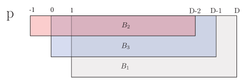
Figure 1: Existence conditions of the terms $B_{1},\ B_{2}$ and $B_{3}$ in the action that could be read from Table 2.

In order to find the invariance conditions we must evaluate eq. (A.6) for each term in the different existence regions, taking into account the special values of $D$ and $p$ for which the terms we are considering contain only fields from one of the subspaces $V_{0}$ or $V_{1}$. For instance, if we take $p=0$ we see from eqs. (1) that only the terms $B_{2}$ and $B_{3}$ exist and that $B_{3}$ has only contributions from $V_{1}$. Thus, the invariance conditions read

$$n\leqslant N_{1}+D-1.$$ (A.8a)

For $B_{2}$ instead we should distinguish the following two cases:

$$\left\{\begin{array}[]{lcl}D=3&&n\leqslant\min\{N_{0},N_{1}+1\}\,,\\[5.69046pt] D\neq 3&&n\leqslant\min\{N_{0},N_{1}-1\}+D-3\,.\end{array}\right.$$ (A.8d)

Putting together these two conditions we deduce that for $p=0$ the term $\accentset{(n)}{B}$ is invariant provided that

$$\left\{\begin{array}[]{lcl}D=3&&n\leqslant\min\{N_{0},N_{1}+1\}\,,\\[5.69046pt] D\neq 3&&n\leqslant\min\{N_{0},N_{1}-1\}+D-3\,.\end{array}\right.$$ (A.8g)

Studying in a similar way the different invariance conditions for different values of $p$, we deduce the following conditions:

$$p=0 \left\{\begin{array}[]{lcl}D=3&&n\leqslant\min\{N_{0},N_{1}+1\}\,,\\[5.69046pt] D\neq 3&&n\leqslant\min\{N_{0},N_{1}-1\}+D-3\,,\end{array}\right.$$ (A.9c)

$$1\leqslant p\leqslant D-3 \left\{\begin{array}[]{lcl}D=p+3&&n\leqslant\min\{N_{0},\min\{N_{0},N_{1}-1\}+2\}\,,\\[5.69046pt] D\neq p+3&&n\leqslant\min\{N_{0},N_{1}-1\}+D-p-3\,,\\ \end{array}\right.$$ (A.9f)

$$p=D-2 n\leqslant\min\{N_{0},N_{1}-1\}+1\,,$$ (A.9g)

$$p=D-1 n\leqslant N_{0}\,.$$ (A.9h)

We note that the case $p=-1$ is not realized. For the two allowed cases $N_{1}\pm 1=N_{0}$ the conditions above can be simplified, using the identity

$$\min\{N_{0},N_{1}-1\}=\min\{N_{1}\pm 1,N_{1}-1\}=N_{1}-1\,,$$ (A.10)

as follows:

$$p=0 \left\{\begin{array}[]{lcl}D=3&&n\leqslant N_{0}\\[5.69046pt] D\neq 3&&n\leqslant N_{1}+D-4\end{array}\right.$$ (A.11c)

$$1\leqslant p\leqslant D-3 \left\{\begin{array}[]{lcl}D=p+3&&n\leqslant N_{0}\\[5.69046pt] D\neq p+3&&n\leqslant N_{1}+D-p-4\\ \end{array}\right.$$ (A.11f)

$$p=D-2 n\leqslant N_{1}$$ (A.11g)

$$p=D-1 n\leqslant N_{0}$$ (A.11h)

As an example, we give in Table 3 the solution of the invariance conditions for $D=5$ and different values of $p$ corresponding to the truncated algebras $\mathfrak{g}(2,1)$ and $\mathfrak{g}(2,3)$:

Algebra	$\mathbf{p=0}$	$\mathbf{p=1}$	$\mathbf{p=2}$	$\mathbf{p=3}$	$\mathbf{p=4}$
$\mathfrak{g}(2,1)$	$n\leqslant 2$	$n\leqslant 1$	$n\leqslant 2$	$n\leqslant 1$	$n\leqslant 2$
$\mathfrak{g}(2,3)$	$n\leqslant 4$	$n\leqslant 3$	$n\leqslant 2$	$n\leqslant 3$	$n\leqslant 2$

Table 3: Invariance conditions for the expanded terms $\accentset{(n)}{B}$ under the algebras $\mathfrak{g}(2,1)$ and $\mathfrak{g}(2,3)$.

Appendix B Transformation rules and curvatures of Example 4

For the convenience of the reader, we give in this appendix the definition of the curvatures and the transformation rules of the gauge fields plus curvatures that occur in Example 4, i.e. the case $(D,p;N_{0},N_{1})=(4,0;2,3)$, discussed in the main text.

The transformation rules for the fields corresponding to the generators of the $\mathfrak{g}(2,3)$ algebra are given by

$$\delta\accentset{(1)}{E}^{a} =d\accentset{(1)}{\epsilon}^{a}-\accentset{(1)}{\lambda}^{a}\accentset{(0)}{\tau}+\accentset{(0)}{\lambda}\accentset{(1)}{\Omega}^{a}-\accentset{(0)}{\lambda}^{ab}\accentset{(1)}{E}_{b}+\accentset{(1)}{\epsilon}_{b}\accentset{(0)}{\Omega}^{ab}\,,$$ (B.1a)

$$\delta\accentset{(3)}{E}^{a} =d\accentset{(3)}{\epsilon}^{a}-\accentset{(3)}{\lambda}^{a}\accentset{(0)}{\tau}+\accentset{(0)}{\lambda}\accentset{(3)}{\Omega}^{a}-\accentset{(1)}{\lambda}^{a}\accentset{(2)}{\tau}+\accentset{(2)}{\lambda}\accentset{(1)}{\Omega}^{a}-\accentset{(0)}{\lambda}^{ab}\accentset{(3)}{E}_{b}+\accentset{(3)}{\epsilon}_{b}\accentset{(0)}{\Omega}^{ab}-\accentset{(2)}{\lambda}^{ab}\accentset{(1)}{E}_{b}+\accentset{(1)}{\epsilon}_{b}\accentset{(2)}{\Omega}^{ab}\,,$$ (B.1b)

$$\delta\accentset{(1)}{\Omega}^{a} =d\accentset{(1)}{\lambda}^{a}-\accentset{(0)}{\lambda}^{ab}\accentset{(0)}{\Omega}_{b}+\accentset{(1)}{\lambda}_{b}\accentset{(0)}{\Omega}^{ab}\,,$$ (B.1c)

$$\delta\accentset{(3)}{\Omega}^{a} =d\accentset{(1)}{\lambda}^{a}-\accentset{(0)}{\lambda}^{ab}\accentset{(0)}{\Omega}_{b}+\accentset{(1)}{\lambda}_{b}\accentset{(0)}{\Omega}^{ab}-\accentset{(2)}{\lambda}^{ab}\accentset{(1)}{\Omega}_{b}+\accentset{(1)}{\lambda}_{b}\accentset{(2)}{\Omega}^{ab}\,,$$ (B.1d)

$$\delta\accentset{(0)}{\Omega}^{ab} =d\accentset{(0)}{\lambda}^{ab}+\accentset{(0)}{\lambda}^{ad}\accentset{(0)}{\Omega}^{b}_{\phantom{b}d}-\accentset{(0)}{\lambda}^{bd}\accentset{(0)}{\Omega}^{a}_{\phantom{b}d}\,,$$ (B.1e)

$$\delta\accentset{(2)}{\Omega}^{ab} =d\accentset{(2)}{\lambda}^{ab}+\accentset{(0)}{\lambda}^{ad}\accentset{(2)}{\Omega}^{b}_{\phantom{b}d}-\accentset{(0)}{\lambda}^{bd}\accentset{(2)}{\Omega}^{a}_{\phantom{b}d}+\accentset{(2)}{\lambda}^{ad}\accentset{(0)}{\Omega}^{b}_{\phantom{b}d}-\accentset{(2)}{\lambda}^{bd}\accentset{(0)}{\Omega}^{a}_{\phantom{b}d}-2\accentset{(1)}{\lambda}^{[a}\accentset{(1)}{\Omega}^{b]}\,,$$ (B.1f)

$$\delta\accentset{(0)}{\tau} =d\accentset{(0)}{\lambda}\,,$$ (B.1g)

$$\delta\accentset{(2)}{\tau} =d\accentset{(2)}{\lambda}-\accentset{(1)}{\lambda}^{a}\accentset{(1)}{E}_{a}+\accentset{(1)}{\epsilon}^{a}\accentset{(1)}{\Omega}_{a}\,.$$ (B.1h)

The curvatures that transform covariantly under these gauge transformations are given by

$$\accentset{(0)}{R}^{ab}(J) =d\accentset{(0)}{\Omega}^{ab}-\accentset{(0)}{\Omega}^{ac}\wedge\accentset{(0)}{\Omega}^{b}_{\phantom{b}c}\,,$$ (B.2a)

$$\accentset{(2)}{R}^{ab}(J) =d\accentset{(2)}{\Omega}^{ab}-\accentset{(0)}{\Omega}^{ac}\wedge\accentset{(2)}{\Omega}^{b}_{\phantom{b}c}\accentset{(2)}{\Omega}^{ac}\wedge\accentset{(2)}{\Omega}^{b}_{\phantom{b}c}-\accentset{(1)}{\Omega}^{a}\wedge\accentset{(1)}{\Omega}^{b}\,,$$ (B.2b)

$$\accentset{(1)}{R}^{a}(G) =d\accentset{(1)}{\Omega}^{a}++\accentset{(0)}{\Omega}^{ab}\wedge\accentset{(1)}{\Omega}^{a}\,,$$ (B.2c)

$$\accentset{(3)}{R}^{a}(G) =d\accentset{(3)}{\Omega}^{a}++\accentset{(0)}{\Omega}^{ab}\wedge\accentset{(3)}{\Omega}^{a}+\accentset{(2)}{\Omega}^{ab}\wedge\accentset{(1)}{\Omega}^{a}\,,$$ (B.2d)

$$\accentset{(1)}{R}^{a}(P) =d\accentset{(1)}{E}^{a}+\accentset{(0)}{\Omega}^{ab}\wedge\accentset{(1)}{E}_{b}-\accentset{(1)}{\Omega}^{a}\wedge\accentset{(0)}{\tau}\,,$$ (B.2e)

$$\accentset{(3)}{R}^{a}(P) =d\accentset{(3)}{E}^{a}+\accentset{(0)}{\Omega}^{ab}\wedge\accentset{(3)}{E}_{b}+\accentset{(2)}{\Omega}^{ab}\wedge\accentset{(1)}{E}_{b}-\accentset{(3)}{\Omega}^{a}\wedge\accentset{(0)}{\tau}-\accentset{(1)}{\Omega}^{a}\wedge\accentset{(2)}{\tau}\,,$$ (B.2f)

$$\accentset{(0)}{R}(H) =d\accentset{(0)}{\tau}\,,$$ (B.2g)

$$\accentset{(2)}{R}(H) =d\accentset{(2)}{\tau}+\accentset{(1)}{\Omega}^{a}\wedge\accentset{(1)}{E}_{a}\,.$$ (B.2h)

These curvatures transform as follows under the gauge transformations (B.1) of the gauge fields:

$$\delta\accentset{(1)}{R}^{a}(P) =-\accentset{(1)}{\lambda}^{a}\accentset{(0)}{R}(H)+\accentset{(0)}{\lambda}\accentset{(1)}{R}^{a}(G)-\accentset{(0)}{\lambda}^{ab}\accentset{(1)}{R}_{b}(P)+\accentset{(1)}{\epsilon}_{b}\accentset{(0)}{R}^{ab}(J)\,,$$ (B.3a)

$$\delta\accentset{(3)}{R}^{a}(P) =-\accentset{(3)}{\lambda}^{a}\accentset{(0)}{R}(H)+\accentset{(0)}{\lambda}\accentset{(3)}{R}^{a}(G)-\accentset{(1)}{\lambda}^{a}\accentset{(2)}{R}(H)+\accentset{(2)}{\lambda}\accentset{(1)}{R}^{a}(G)-\accentset{(0)}{\lambda}^{ab}\accentset{(3)}{R}_{b}(P)+\accentset{(3)}{\epsilon}_{b}\accentset{(0)}{R}^{ab}(J)$$

$$-\accentset{(2)}{\lambda}^{ab}\accentset{(1)}{R}_{b}(P)+\accentset{(1)}{\epsilon}_{b}\accentset{(2)}{R}^{ab}(J)\,,$$ (B.3b)

$$\delta\accentset{(1)}{R}^{a}(G) =-\accentset{(0)}{\lambda}^{ab}\accentset{(1)}{R}_{b}(G)+\accentset{(1)}{\lambda}_{b}\accentset{(0)}{R}^{ab}(J)\,,$$ (B.3c)

$$\delta\accentset{(3)}{R}^{a}(G) =-\accentset{(0)}{\lambda}^{ab}\accentset{(3)}{R}_{b}(G)+\accentset{(3)}{\lambda}_{b}\accentset{(0)}{R}^{ab}(J)-\accentset{(2)}{\lambda}^{ab}\accentset{(1)}{R}_{b}(G)+\accentset{(1)}{\lambda}_{b}\accentset{(2)}{R}^{ab}(J)\,,$$ (B.3d)

$$\delta\accentset{(0)}{R}^{ab}(J) =\accentset{(0)}{\lambda}^{ad}\accentset{(0)}{R}^{b}_{\phantom{b}d}(J)-\accentset{(0)}{\lambda}^{bd}\accentset{(0)}{R}^{a}_{\phantom{b}d}(J)\,,$$ (B.3e)

$$\delta\accentset{(2)}{R}^{ab}(J) =\accentset{(0)}{\lambda}^{ad}\accentset{(2)}{R}^{b}_{\phantom{b}d}(J)-\accentset{(0)}{\lambda}^{bd}\accentset{(2)}{R}^{a}_{\phantom{b}d}(J)+\accentset{(2)}{\lambda}^{ad}\accentset{(0)}{R}^{b}_{\phantom{b}d}(J)-\accentset{(2)}{\lambda}^{bd}\accentset{(0)}{R}^{a}_{\phantom{b}d}(J)-2\accentset{(1)}{\lambda}^{[a}\accentset{(1)}{R}^{b]}(G)\,,$$ (B.3f)

$$\delta\accentset{(0)}{R}(H) =0\,,$$ (B.3g)

$$\delta\accentset{(2)}{R}(H) =-\accentset{(1)}{\lambda}^{a}\accentset{(1)}{R}_{a}(P)+\accentset{(1)}{\epsilon}^{a}\accentset{(1)}{R}_{a}(G)\,.$$ (B.3h)

References

• [1] A. Bagchi and R. Gopakumar, “Galilean Conformal Algebras and AdS/CFT,” JHEP 0907 (2009) 037 DOI:10.1088/1126-6708/2009/07/037 [arXiv:0902.1385 [hep-th]];
• [2] M. H. Christensen, J. Hartong, N. A. Obers and B. Rollier, “Torsional Newton-Cartan Geometry and Lifshitz Holography,” Phys. Rev. D 89 (2014) 061901 DOI:10.1103/PhysRevD.89.061901 [arXiv:1311.4794 [hep-th]].
• [3] D. T. Son, “Newton-Cartan Geometry and the Quantum Hall Effect,” arXiv:1306.0638 [cond-mat.mes-hall];
• [4] M. Geracie, D. T. Son, C. Wu and S. F. Wu, “Spacetime Symmetries of the Quantum Hall Effect,” Phys. Rev. D 91 (2015) 045030 DOI:10.1103/PhysRevD.91.045030 [arXiv:1407.1252 [cond-mat.mes-hall]].
• [5] E. Bergshoeff, J. Gomis, B. Rollier, J. Rosseel and T. ter Veldhuis, “Carroll versus Galilei Gravity,” JHEP 1703 (2017) 165 DOI:10.1007/JHEP03(2017)165 [arXiv:1701.06156 [hep-th]].
• [6] G. Papageorgiou and B. J. Schroers, “A Chern-Simons approach to Galilean quantum gravity in 2+1 dimensions,” JHEP 0911 (2009) 009 DOI:10.1088/1126-6708/2009/11/009 [arXiv:0907.2880 [hep-th]].
• [7] E. A. Bergshoeff and J. Rosseel, “Three-Dimensional Extended Bargmann Supergravity,” Phys. Rev. Lett.  116 (2016) no.25, 251601 DOI:10.1103/PhysRevLett.116.251601 [arXiv:1604.08042 [hep-th]].
• [8] J. Hartong, Y. Lei and N. A. Obers, “Nonrelativistic Chern-Simons theories and three-dimensional Horava-Lifshitz gravity,” Phys. Rev. D 94 (2016) no.6, 065027 DOI:10.1103/PhysRevD.94.065027 [arXiv:1604.08054 [hep-th]].
• [9] D. Hansen, J. Hartong and N. A. Obers, “An Action Principle for Newtonian Gravity,” Phys. Rev. Lett. 122, 061106 (2019) DOI:10.1103/PhysRevLett.122.061106 [hep-th/1807.04765]; D. Hansen, J. Hartong and N. A. Obers, “Gravity between Newton and Einstein,” arXiv:1904.05706 [gr-qc].
• [10] R. Andringa, E. Bergshoeff, J. Gomis and M. de Roo, “’Stringy’ Newton-Cartan Gravity,” Class. Quant. Grav.  29 (2012) 235020 DOI:10.1088/0264-9381/29/23/235020 [arXiv:1206.5176 [hep-th]].
• [11] J. Brugues, T. Curtright, J. Gomis and L. Mezincescu, “Non-relativistic strings and branes as non-linear realizations of Galilei groups,” Phys. Lett. B 594 (2004) 227 DOI:10.1016/j.physletb.2004.05.024 [hep-th/0404175].
• [12] E. Bergshoeff, J. Gomis and Z. Yan, “Nonrelativistic String Theory and T-Duality,” JHEP 1811 (2018) 133 DOI:10.1007/JHEP11(2018)133 [arXiv:1806.06071 [hep-th]].
• [13] J. Gomis and H. Ooguri, “Nonrelativistic closed string theory,” J. Math. Phys.  42 (2001) 3127 DOI:10.1063/1.1372697 [hep-th/0009181].
• [14] B. Julia and H. Nicolai, “Null Killing vector dimensional reduction and Galilean geometrodynamics,” Nucl. Phys. B 439 (1995) 291 DOI:10.1016/0550-3213(94)00584-2 [hep-th/9412002].
• [15] E. A. Bergshoeff, K. T. Grosvenor, C. Simsek and Z. Yan, “An Action for Extended String Newton-Cartan Gravity,” JHEP 1901 (2019) 178 DOI:10.1007/JHEP01(2019)178 [arXiv:1810.09387 [hep-th]].
• [16] N. Ozdemir, M. Ozkan, O. Tunca and U. Zorba, “Extended Newtonian (Super)Gravity,” arXiv:1903.09377 [hep-th].
• [17] M. Hatsuda and M. Sakaguchi, “Wess-Zumino term for the AdS superstring and generalized Inönü-Wigner contraction,” Prog. Theor. Phys.  109 (2003) 853 DOI:10.1143/PTP.109.853 [hep-th/0106114].
• [18] J. A. de Azcárraga, J. M. Izquierdo, M. Picón and O. Varela, “Generating Lie and gauge free differential (super)algebras by expanding Maurer-Cartan forms and Chern-Simons supergravity,” Nucl. Phys. B 662 (2003) 185 DOI:10.1016/S0550-3213(03)00342-0 [hep-th/0212347].
• [19] J. A. de Azcárraga, J. M. Izquierdo, M. Picón and O. Varela, “Expansions of algebras and superalgebras and some applications,” Int. J. Theor. Phys. 46 (2007) 2738-2752 DOI:10.1007/s10773-007-9385-3 [hep-th/0703017].
• [20] F. Izaurieta, E. Rodríguez and P. Salgado, “Expanding Lie (super)algebras through Abelian semigroups,” J. Math. Phys.  47 (2006) 123512 DOI:10.1063/1.2390659 [hep-th/0606215].
• [21] J. A. de Azcárraga and J. M. Izquierdo, “(p,q) D=3 Poincaré supergravities from Lie algebra expansions,” Nucl. Phys. B 854 (2012) 276 DOI:10.1016/j.nuclphysb.2011.08.020 [arXiv:1107.2569 [hep-th]].
• [22] J. A. de Azcarraga, J. M. Izquierdo, J. Lukierski and M. Woronowicz, “Generalizations of Maxwell (super)algebras by the expansion method,” Nucl. Phys. B 869 (2013) 303 doi:10.1016/j.nuclphysb.2012.12.008 [arXiv:1210.1117 [hep-th]].
• [23] P. K. Concha and E. K. Rodríguez, “Maxwell Superalgebras and Abelian Semigroup Expansion,” Nucl. Phys. B 886 (2014) 1128 doi:10.1016/j.nuclphysb.2014.07.022 [arXiv:1405.1334 [hep-th]].
• [24] L. Avilés, E. Frodden, J. Gomis, D. Hidalgo and J. Zanelli, “Non-Relativistic Maxwell Chern-Simons Gravity,” JHEP 1805 (2018) 047 doi:10.1007/JHEP05(2018)047 [arXiv:1802.08453 [hep-th]].
• [25] J. Gomis and A. Kleinschmidt, “On free Lie algebras and particles in electro-magnetic fields,” JHEP 1707 (2017) 085 doi:10.1007/JHEP07(2017)085 [arXiv:1705.05854 [hep-th]].
• [26] J. M. Izquierdo, “Lie algebra expansions and three-dimensional Galilean supergravity”, talk given at the Spanish-Portuguese Relativity Meeting (EREP) Palencia, Spain, September 2018; J. A. de Azcárraga, D. Gútiez and J. M. Izquierdo, “Extended $D=3$ Bargmann supergravity from a Lie algebra expansion,” arXiv:1904.12786 [hep-th].
• [27] T. Harmark, J. Hartong, L. Menculini, N. A. Obers and Z. Yan, “Strings with Non-Relativistic Conformal Symmetry and Limits of the AdS/CFT Correspondence,” JHEP 1811 (2018) 190 DOI:10.1007/JHEP11(2018)190 [arXiv:1810.05560 [hep-th]].
• [28] E.A. Bergshoeff, J. Rosseel, C. Şimşek, Z. Yan, “Spacetime Geometry and Nonrelativistic String Theory,” in preparation.
• [29] D. Van den Bleeken, “Torsional Newton-Cartan gravity from the large c expansion of general relativity,” Class. Quant. Grav.  34 (2017) no.18, 185004 DOI:10.1088/1361-6382/aa83d4 [arXiv:1703.03459 [gr-qc]]; “Torsional Newton-Cartan gravity and strong gravitational fields,” arXiv:1903.10682 [gr-qc].
• [30] P. D. Álvarez, J. Gomis, K. Kamimura and M. S. Plyushchay, “(2+1)D Exotic Newton-Hooke Symmetry, Duality and Projective Phase,” Annals Phys.  322 (2007) 1556 DOI:10.1016/j.aop.2007.03.002 [hep-th/0702014].
• [31] O. Khasanov and S. Kuperstein, “(In)finite extensions of algebras from their Inonu-Wigner contractions,” J. Phys. A 44 (2011) 475202 DOI:10.1088/1751-8113/44/47/475202 [arXiv:1103.3447 [hep-th]].
• [32] M. Henneaux, “Geometry of Zero Signature Space-times,” Bull. Soc. Math. Belg.  31 (1979) 47.
• [33] E. Bergshoeff, D. Grumiller, S. Prohazka and J. Rosseel, “Three-dimensional Spin-3 Theories Based on General Kinematical Algebras,” JHEP 1701 (2017) 114 DOI:10.1007/JHEP01(2017)114 arXiv:1612.02277 [hep-th]].