Waterfall Bandits: Learning to Sell Ads Online

Abstract

A popular approach to selling online advertising is by a waterfall, where a publisher makes sequential price offers to ad networks for an inventory, and chooses the winner in that order. The publisher picks the order and prices to maximize her revenue. A traditional solution is to learn the demand model and then subsequently solve the optimization problem for the given demand model. This will incur a linear regret. We design an online learning algorithm for solving this problem, which interleaves learning and optimization, and prove that this algorithm has sublinear regret. We evaluate the algorithm on both synthetic and real-world data, and show that it quickly learns high-quality pricing strategies. This is the first principled study of learning a waterfall design online by sequential experimentation.

1 Introduction

Online publishers typically generate revenue by placing advertisements. For example, when a user visits a webpage, there are locations called slots each of which may have an impression of an advertisement (ad).

• A slot may be sold directly to a specific brand advertiser. In that case, when a user arrives at the webpage, the publisher calls the advertiser and places the ad returned as the impression.

• A slot may be sold via third parties such as Google’s DoubleClick Ad Exchange. In this case, when a user arrives at the webpage, the publisher calls the ad exchange which in turn calls many intermediaries called ad networks. Each ad network has several advertisers as its customers and bids on behalf of one of its chosen customers. The ad exchange runs an auction among the bids and returns the winner to the publisher which becomes the ad impression for the user.

• A slot may be sold directly to different ad networks. In this case, publishers typically run what is a called a waterfall. In the waterfall, the publisher chooses a permutation of the ad networks. The publisher calls each ad network sequentially according to the permutation and offers a price. The ad network has to bid above that price to win the opportunity to place the ad at that slot. If the ad network does not make an adequate bid, the slot is offered to the next ad network and so on. The publisher gets to choose the permutation and reserve prices.

The three methods above trade off between control, margins and relationships between publishers, ad networks and advertisers. Often publishers combine these methods. For example, publishers might use direct deals for premium slots (like top of homepages), use waterfall variants for torso inventory, and Ad Exchanges for tail or remnant slots that did not get sold by the other methods. Readers who wish more background on the ad business and the role of waterfalls can see [19, 17] or see DoubleClick’s support pages .

In this paper, we address the central question how publishers can design the waterfall. We formalize this problem as learning the optimal order of ad networks with their offered prices. Our objective is to maximize the expected revenue of the publisher online in a sequence of $n$ steps, which is equivalent to minimizing the expected regret with respect to the best solution in hindsight.

• We formalize and study the problem of publisher learning and optimizing ad revenue from waterfall design as an online learning problem with partial feedback.

• We develop a bandit style solution and propose a computationally-efficient UCB-like algorithm for this problem, which we call ${\tt WaterfallUCB1}$. Our learning problem is challenging for two reasons. First, the space of feasible solutions, all permutations of ad networks and their offered prices, is exponentially large. Second, our problem suffers from partial feedback, which is similar to that in cascading bandits [11, 12]. In particular, if an ad network accepts an offer, the learning agent does not learn if any of the subsequent ad networks would have accepted their offered prices.

• We prove an upper bound on the expected $n$-step regret of algorithm ${\tt WaterfallUCB1}$. The upper bound is sublinear in $n$ and polynomial in all other quantities of interest. The key step in our analysis is a new regret decomposition, which is of independent interest beyond our motivating domain of online advertising.

• We conduct extensive experiments on both synthetic and real-world data, which show that ${\tt WaterfallUCB1}$ learns high-quality solutions. In addition, we investigate several practical settings that are encountered by publishers:

  • Publishers typically have many web pages with multiple ad slots per page. We show with real-world data that waterfall learning for all ad slots yields good solutions when the ad networks behave similarly across the ad slots.

  • Instead of going directly to ad networks, publishers can go to third parties that aggregate over ad networks. We show our algorithm ${\tt WaterfallUCB1}$ can also learn to sell in this setting and it does not overfit.

Taken together, the above represents the first principled study of publisher revenue when using waterfall to optimize ad placement.

2 Selling in the Waterfall

The problem of selling one ad slot in the waterfall can be formalized as follows. Let $[K]=\{1,\dots,K\}$ be a set of $K$ ad networks. Let $Q=\{q_{1},\dots,q_{M}\}$ be a set of $M$ prices, where $q_{i}\geq 0$ for all $i\in[M]$. We use discrete prices as in [6]; they are a first reasonable approach for the waterfall. We will discuss this further in Section 5. Then any instance of our problem can be defined by a tuple $(K,Q,(\mathbb{P}_{a})_{a\in[K]})$, where $\mathbb{P}_{a}$ is a probability distribution over the valuation of ad network $a$. Without loss of generality, we assume that all prices in $Q$ are in $[0,1]$, and that the support of $\mathbb{P}_{a}$ is a subset of $[0,1]$ for all $a\in[K]$. We assume that the valuation of any ad network $a$, $v_{a}\sim\mathbb{P}_{a}$, is drawn independently from the valuations of all other ad networks.

The publisher sells to the ad networks as follows. First, it chooses a permutation of the ad networks $(a_{1},\dots,a_{K})\in\Pi(K)$ and offered price $p_{i}\in Q$ for each ad network $a_{i}$, where $\Pi(K)$ is the set of all permutations of $[K]$. Then the publisher contacts the ad networks sequentially, from $a_{1}$ to $a_{K}$, and tries to sell the ad slot to them. In particular:

• Ad network $a_{1}$ is contacted first.

• If ad network $a_{i}$ is contacted and $p_{i}\leq v_{a_{i}}$, the offered price is lower than or equal to the valuation of ad network $a_{i}$, the offer is accepted. Then the publisher earns $p_{i}$ and does not contact any of the remaining ad networks.

• If ad network $a_{i}$ is contacted and $p_{i}>v_{a_{i}}$, the offered price is higher than the valuation of ad network $a_{i}$, the offer is rejected. Then the publisher contacts ad network $a_{i+1}$ if $i<K$. If $i=K$, the publisher does not sell the ad slot and earns zero.

We denote by $A=((a_{i})_{i\in[K]},(p_{i})_{i\in[K]})$ the action of the publisher. The set of feasible actions is $\mathcal{A}=\Pi(K)\times Q^{K}$. For any ad network $a\in[K]$ and price $p\in Q$, we define acceptance probability $\bar{w}(a,p)=P(p\leq v_{a})$, the probability that ad network $a$ accepts price $p$ under valuation distribution $\mathbb{P}_{a}$. We refer to any pair of the ad network and price, $(a,p)$ for $a\in[K]$ and $p\in Q$, as an item; and define the set of all items as $E=[K]\times Q$. Note that $|E|=KM$. For any action $A=((a_{i})_{i\in[K]},(p_{i})_{i\in[K]})\in\mathcal{A}$ and weight function $u:[K]\times Q\to[0,1]$, we define

$$f(A,u)=\sum_{i=1}^{K}\left[\prod_{k=1}^{i-1}[1-u(a_{j},p_{j})]\right]u(a_{i},p_{i})\,p_{i}\,.$$ (1)

This is the expected revenue of the publisher under action $A$ and acceptance probabilities $u$. In particular, assuming the valuations of ad networks are independent, $\prod_{j=1}^{i-1}[1-u(a_{j},p_{j})]$ is the probability that all ad networks before ad network $a_{i}$ do not accept their offered prices, which is equal to the probability that $a_{i}$ is contacted. Moreover, $u(a_{i},p_{i})$ is the conditional probability of ad network $a_{i}$ accepting its offered price $p_{i}$ after it is contacted. The objective of the publisher is to maximize its expected revenue by choosing $A\in\mathcal{A}$,

$$A^{\ast}=\arg\max_{A\in\mathcal{A}}f(A,\bar{w})\,.$$ (2)

We refer to $A^{\ast}$ as the optimal solution.

2.1 Oracles

No polynomial-time algorithm is known for solving all instances of problem (2). However, computationally-efficient approximations exist [6, 7]. In this work, we consider approximation algorithms $L$ whose inputs are a weight function $u:[K]\times Q\to[0,1]$, the number of ad networks $K$, and a set of prices $Q$; and the output is $L(u,K,Q)\in\mathcal{A}$. We say that algorithm $L$ is a $\gamma$-approximation for $\gamma\in(0,1]$ if $f(L(u,K,Q),u)\geq\gamma\max_{A\in\mathcal{A}}f(A,u)$ for any $u$.

Note that when ad networks are assigned prices, the optimal order of the ad networks is in the descending order of their assigned prices. This follows from the definition of the revenue in (1). Since the output of $L$ can be always ordered to satisfy this property, we assume that this property is satisfied without loss of generality. We consider two oracles in this paper, greedy and based on linear programming (LP).

Algorithm 1 Greedy oracle.

0:  Weight function $u$, number of ad networks $K$, prices $Q$

  

  for all $a\in[K]$ do

     $p^{\ast}(a)\leftarrow\arg\max_{p\in Q}u(a,p)\,p$

  Let $\pi$ be any permutation of $[K]$ such that $p^{\ast}(\pi(1))\geq\ldots\geq p^{\ast}(\pi(K))$

  $A\leftarrow((\pi(i))_{i\in[K]},(p^{\ast}(\pi(i)))_{i\in[K]})$

  

  Publisher action $A$

The pseudocode of the greedy oracle is in Algorithm 1. The oracle has two main stages. First, it assigns to each ad network $a\in[K]$ the price that maximizes the expected revenue of that ad network conditioned on being contacted, $p^{\ast}(a)$. Second, it orders the ad networks in the descending order of their assigned prices. This oracle is easy to implement and performs well in our experiments. It does not have any approximation guarantee though.

Algorithm 2 LP oracle.

0:  Weight function $u$, number of ad networks $K$, prices $Q$

  

  Solve

$$\displaystyle\max\quad \sum_{a=1}^{K}\sum_{p\in Q}p\,y_{a,p}$$

s.t. $$\forall a\in[K],p\in Q:y_{a,p}\leq u(a,p)\,x_{a,p}\,,\ \ x_{a,p}\geq 0\,,\ \ y_{a,p}\geq 0\,;$$

$$\sum_{a=1}^{K}\sum_{p\in Q}y_{a,p}\leq 1\,;\quad\forall a\in[K]:\sum_{p\in Q}x_{a,p}\leq 1;$$

  Let $\tau^{\ast}$ be the dual variable associated with the last constraint of the above LP

  

  for all $a\in[K]$ do

     $p^{\ast}(a)\leftarrow\arg\max_{p\in Q}u(a,p)\,(p-\tau^{\ast})$

     if $(\max_{p\in Q}u(a,p)\,(p-\tau^{\ast})=0)$ and $(\tau^{\ast}\in Q)$ then

        $p^{\ast}(a)\leftarrow\tau^{\ast}$

  Let $\pi$ be any permutation of $[K]$ such that $p^{\ast}(\pi(1))\geq\ldots\geq p^{\ast}(\pi(K))$

  $A\leftarrow((\pi(i))_{i\in[K]},(p^{\ast}(\pi(i)))_{i\in[K]})$

  

  Publisher action $A$

The pseudocode of the LP oracle is in Algorithm 2. The oracle is based on linear programming and is a $(1-\frac{1}{e})$-approximation algorithm [6]. The oracle has three main stages. First, it solves an LP to obtain the value of the dual variable corresponding to the last constraint $\tau^{\ast}$. Second, it assigns to each ad network $a\in[K]$ the price $p$ that maximizes $u(a,p)\,(p-\tau^{\ast})$. This price is denoted by $p^{\ast}(a)$. Finally, it orders the ad networks in the descending order of their assigned prices.

The optimized variables in the linear program are $x_{a,p}$ and $y_{a,p}$, for $a\in[K]$ and $p\in Q$. The variable $x_{a,p}$ represents the probability that ad network $a$ is offered price $p$. The variable $y_{a,p}$ represents the joint probability that ad network $a$ is offered price $p$ and accepts. The objective is the expected return. The constraints guarantee that the probabilities are consistent and non-negative.

Both discussed oracles can find high-quality strategies for selling a single ad slot in the waterfall. In practice, publishers may be interested in maximizing the revenue from all of their many ad slots. We return to these practical issues in Section 6.

3 Waterfall Bandit

As we discussed earlier, publishers often do not know the valuation distributions of ad networks in advance. However, since they repeatedly sell ad slots to the ad networks, they can learn it. This motivates our study of the waterfall as a multi-armed bandit (MAB) [14, 3], which we call a waterfall bandit. Formally, the waterfall bandit is a tuple $(K,Q,(\mathbb{P}_{a})_{a\in[K]})$, where the valuation distributions of ad networks $(\mathbb{P}_{a})_{a\in[K]}$ are unknown to the publisher. Let $v_{t,a}\sim\mathbb{P}_{a}$ be the stochastic valuation of ad network $a$ at time $t$. We assume that $v_{t,a}$ is drawn independently from $\mathbb{P}_{a}$, both across ad networks and in time.

The publisher repeatedly sells to ad networks for $n$ times. At each time $t$, based on past observations, the publisher adaptively chooses action $A_{t}=((a_{t,i})_{i\in[K]},(p_{t,i})_{i\in[K]})$, where $a_{t,i}\in[K]$ and $p_{t,i}\in Q$ are the $i$-th contacted ad network at time $t$ and its assigned price, respectively. The publisher receives feedback $B_{t}\in[K]\cup\{\infty\}$, which is the index of the first ad network that accepts its offered price. In particular, when $B_{t}=i$ for $i\in[K]$, ad network $a_{t,i}$ accepts its offered price $p_{t,i}$ and the reward of the publisher is $p_{t,i}$. On the other hand, when $B_{t}=\infty$, no ad network accepts its offered price and the reward of the publisher is zero. Because the ad networks are contacted sequentially, the publisher knows that the offered price $p_{t,i}$ is not accepted by any ad network $a_{t,i}$ such that $i<B_{t}$ for $i\in[K]$. In summary, the publisher observes responses from all ad networks $a_{t,i}$ such that $i\leq B_{t}$ for $i\in[K]$, and we refer to these ad networks as being observed.

We evaluate the performance in the waterfall bandit by a form of regret, where the cumulative reward of the optimal solution $A^{\ast}$ is weighted by a factor of $\gamma$. In particular, the scaled $n$-step regret is defined as

$$R^{\gamma}(n)=n\gamma f(A^{\ast},\bar{w})-\mathbb{E}\left[\sum_{t=1}^{n}f(A_{t},\bar{w})\right]\,,$$ (3)

where $\gamma>0$ is the aforementioned scaling factor and $A^{\ast}$ is the optimal solution in (2). The reason for the scaling factor is that no polynomial-time algorithms exists for solving our offline optimization problem (Section 2.1). Therefore, it is unreasonable to assume that we can learn such solutions online, and it is reasonable to compete with the best offline $\gamma$-approximation. Note that the scaled $n$-step regret reduces to the standard $n$-step regret when $\gamma=1$.

Naive Solutions. The waterfall bandit can be solved as a multi-armed bandit problem where the expected revenue of each action $A\in\mathcal{A}$ is estimated separately. This solution would not be statistically efficient. The reason is that the number of actions is $|\mathcal{A}|=K!M^{K}$, and so a naive unstructured solution would have exponential regret in $K$.

The key structure in our learning problem is that the publisher receives feedback on individual ad networks in each action. This setting is reminiscent of stochastic combinatorial semi-bandits [9, 8, 13, 18], which can be solved statistically efficiently. The challenge is that the publisher may not receive feedback on all ad networks. More specifically, when $a_{t,i}>B_{t}$ at time $t$, the publisher does not know if ad network $a_{t,i}$ would accepted price $p_{t,i}$ if it was offered that price. Therefore, our problem cannot be formulated and solved as a stochastic combinatorial semi-bandit.

A similar form of partial feedback was studied in cascading bandits [11], where the learning agent receives feedback on a ranked list of items, for all items in the list up to the first clicked item. The difference in our setting is that Kveton et al. [11] do not consider pricing. Nevertheless, it is reasonable to assume that a similar learning algorithm, which maintains upper confidence bounds on all acceptance probabilities $\bar{w}(a,p)$, for any $a\in[K]$ and $p\in Q$, could solve our problem. We present such an algorithm in Section 4.

4 ${\tt WaterfallUCB1}$ Algorithm

In this section, we propose a UCB-like algorithm for the waterfall bandit, which we call ${\tt WaterfallUCB1}$. The algorithm is presented in Algorithm 3.

The inputs to ${\tt WaterfallUCB1}$ are an approximation oracle $L$, the number of ad networks $K$, and a set of prices $Q$. At each time $t$, ${\tt WaterfallUCB1}$ proceeds as follows. First, it computes an upper confidence bound (UCB) $U_{t}(e)=\min\{\hat{w}_{T_{t-1}(e)}(e)+c_{t-1,T_{t-1}(e)},1\}$ on the acceptance probability $\bar{w}(e)$ of all $e=(a,p)\in E$, where $E$ is the set of all ad-network and price pairs (Section 2), $\hat{w}_{s}(e)$ is the fraction of accepted offers in $s$ trials when ad network $a$ is offered price $p$, $T_{t}(e)$ is the number of times that ad network $a$ is offered price $p$ up to time $t$, and $c_{t,s}=\sqrt{(1.5\log t)/s}$ is the radius of a confidence interval around $\hat{w}_{s}(e)$ after $t$ steps such that $\bar{w}(e)\in[\hat{w}_{s}(e)-c_{t,s},\hat{w}_{s}(e)+c_{t,s}]$ holds with a high probability. We trim $U_{t}(e)$ at $1$ so that it can be interpreted as a probability.

After the UCBs are computed, ${\tt WaterfallUCB1}$ computes its action at time $t$, $A_{t}=((a_{t,i})_{i\in[K]},(p_{t,i})_{i\in[K]})$, using the oracle $L$ and UCBs $U_{t}$. Then it takes that action and receives feedback $B_{t}$. Finally, ${\tt WaterfallUCB1}$ updates its statistics for all observed pairs of ad networks and prices, $(a_{t,i},p_{t,i})$ such that $i\leq\min\{B_{t},K\}$.

Algorithm 3 Algorithm ${\tt WaterfallUCB1}$.

0:  Oracle $L$, number of ad networks $K$, prices $Q$

  

  for all $e=(a,p)\in E$ do // Initialization

     Offer price $p$ to ad network $a$ once

     $\hat{w}_{0}(e)\leftarrow\mathbb{1}\{\text{$a$ accepts price $p$}\},\ T_{0}(e)\leftarrow 1$

  

  for $t=1,\dots,n$ do

     for all $e=(a,p)\in E$ do // Compute UCBs

        $U_{t}(e)=\min\{\hat{w}_{T_{t-1}(e)}(e)+c_{t-1,T_{t-1}(e)},1\}$

     $A_{t}\leftarrow L(U_{t},K,Q)$ // Compute the action using the oracle and $U_{t}$

     Observe $B_{t}\in\{1,\dots,K,+\infty\}$ // Run the waterfall and get feedback

     

     $T_{t}(e)\leftarrow T_{t-1}(e)$, $\forall e\in E$ // Update statistics

     for $i=1,\dots,\min\{B_{t},K\}$ do

        $e\leftarrow(a_{t,i},p_{t,i})$

        $T_{t}(e)\leftarrow T_{t}(e)+1$

        $\displaystyle\hat{w}_{T_{t}(e)}(e)\leftarrow\frac{T_{t-1}(e)\hat{w}_{T_{t-1}(e)}(e)+\mathbb{1}\{B_{t}=i\}}{T_{t}(e)}$

5 Analysis

The regret of ${\tt WaterfallUCB1}$ is bounded in the following theorem.

Theorem 1.

Let ${\tt WaterfallUCB1}$ be run in the waterfall bandit with a $\gamma$-approximation oracle $L$. Then $R^{\gamma}(n)\leq 4MK\sqrt{1.5n\log n}+\gamma\frac{\pi^{2}}{3}MK\,,$ where $K$ is the number of ad networks and $M$ is the number of prices in $Q$.

Proof.

We sketch the proof of Theorem 1 below. The detailed proof is in Appendix A.

The proof proceeds as follows. First, we show that $f(A,u)$ is monotone in weight function $u$ for any fixed action $A$ (Lemma 5 in Appendix A). Second, based on this monotonicity property, we bound the per-step scaled regret at time $t$, $R_{t}^{\gamma}=\gamma f(A^{\ast},\bar{w})-f(A_{t},\bar{w})$, under “good event” $\bar{\mathcal{E}}_{t}$, that all $\bar{w}(e)$ are inside of their confidence intervals at time $t$. This novel regret decomposition is presented in Lemma 5 below.

lemmalemmadecomp Conditioned on “good event” $\bar{\mathcal{E}}_{t}$, the per-step scaled regret at time $t$ is bounded as $R_{t}^{\gamma}\leq\sum_{i=1}^{K}\mathbb{E}_{t}\left[\mathbb{1}\{G_{d_{t,i},t}\}\right]\phi_{d_{t,i},t}\,,$ where $d_{t,i}=(a_{t,i},p_{t,i})$, $\phi_{e,t}=U_{t}(e)-\bar{w}(e)$, and $G_{e,t}$ is the event that item $e$ is observed at time $t$.

The proof of Lemma 5 is in Appendix A. Note that the lemma decomposes the regret at time $t$ into those of observed items. Based on the definition of “good event” $\bar{\mathcal{E}}_{t}$ and some algebra, we have $\sum_{t=1}^{n}\mathbb{E}[\mathbb{1}\{\bar{\mathcal{E}}_{t}\}R^{\gamma}_{t}]\leq 2\sqrt{1.5\log n}\sum_{e\in E}\sum_{t=1}^{n}\frac{1}{\sqrt{t}}\leq 4MK\sqrt{1.5\,n\log n}\,.$ On the other hand, we bound the regret under “bad event” $\mathcal{E}_{t}$, that at least one $\bar{w}(e)$ is outside of its confidence interval, using Hoeffding’s inequality. Specifically, we get $\sum_{t=1}^{n}\mathbb{E}[\mathbb{1}\{\mathcal{E}_{t}\}R^{\gamma}_{t}]\leq\gamma\frac{\pi^{2}}{3}MK$. The bound in Theorem 1 follows directly from combining the above two inequalities. ∎

Theorem 1 provides a $O(MK\sqrt{n\log n})$ gap-free upper bound on the scaled $n$-step regret of ${\tt WaterfallUCB1}$. We discuss the tightness of this bound below. The dependence on $\sqrt{n\log n}$ is standard in gap-free bounds in similar problems [13, 12], and it is considered $O(\sqrt{\log n})$ from being tight. The dependence $MK$ is expected, since ${\tt WaterfallUCB1}$ estimates $MK$ values, one for each ad network and price. However, linear dependence on $MK$ may not be tight. We obtain it for two reasons. First, ${\tt WaterfallUCB1}$ learns $\bar{w}(e)$ separately for each item $e\in E$, and does not exploit any generalization across ad networks and prices. Second, our bound is proved directly from the “self-normalization” of confidence interval radii (Appendix A), not through a gap-dependent bound as in related papers [13, 12].

Our analysis also provides a sublinear regret bound with respect to the optimal continuous-price solution. In particular, let all prices be in $[0,1]$ and suppose the publisher intends to maximize expected revenue up to time $n$. When the prices are discretized on a uniform grid with $M$ points over $[0,1]$, the maximum instantaneous loss due to discretization is $CK/M$, where $C$ is a problem-specific Lipschitz factor. Under this assumption, the scaled $n$-step regret with respect to the optimal continuous-price solution is bounded by $O(MK\sqrt{n\log n}+\gamma MK)+nCK/M$. Now we choose

$$M=\sqrt{nC/(\sqrt{n\log n}+\gamma)}$$

and we get a $O\left(K\sqrt{C\cdot n}\sqrt{\sqrt{n\log n}+\gamma}\right)$ regret bound.

6 Experiments

In this section, we empirically evaluate the effectiveness of our algorithm. We also investigate the settings where our algorithm may be deployed in practice.

6.1 Methods and Metrics

The input to ${\tt WaterfallUCB1}$ is an oracle, which orders ad networks and assigns prices to them for any model $u$ (Section 2.1). We experiment with two oracles, Greedy (Algorithm 1) and LP (Algorithm 2). We compare the following offline and online approaches, where X refers to one of the aforementioned oracles:

1. Offline-X is an offline approximation algorithm. The input to the algorithm are all acceptance probabilities, $\bar{w}(a,p)$ for any $a\in[K]$ and $p\in Q$. The probabilities are used by oracle $X$ to order ad networks and assign prices to them. The ordering and prices are computed only once and used in all steps. Although this approach is unrealistic because it assumes that the acceptance probabilities are known, it is a useful baseline for evaluating revenue loss due to not knowing the dynamics of the system.

2. UCB-X is the ${\tt WaterfallUCB1}$ in Algorithm 3.

3. Exp²-X is an online approximation algorithm, which explores in the first $n_{0}$ steps and then exploits [16]. In the first $n_{0}$ steps, the algorithm offers random prices to randomly ordered ad networks and collects observations. Then it estimates all acceptance probabilities from its observations. The probabilities are used by oracle $X$ to order ad networks and assign prices to them. The ordering and prices are computed in step $n_{0}$ and then used in all remaining steps. The exploration parameter $n_{0}$ tends to be small in practice because random exploration hurts experience.

The performance of all compared algorithms is evaluated by their expected $n$-step reward,

$$r(n)=\frac{1}{n}\sum_{t=1}^{n}\sum_{i=1}^{K}\!\left[\prod_{j=1}^{i-1}\mathbb{1}\!\left\{p_{t,j}>v_{t,a_{t,j}}\right\}\right]\!\mathbb{1}\!\left\{p_{t,i}\leq v_{t,a_{t,i}}\right\}\,p_{t,i}\,,$$

where $A_{t}=\left((a_{t,i})_{i\in[K]},(p_{t,i})_{i\in[K]}\right)$ is the action of the publisher at time $t$ and $v_{t,a}$ is the valuation of ad network $a$ at time $t$. We choose this metric instead of the scaled regret in (3) because the optimal solution to our offline optimization problem cannot be computed efficiently (Section 2.1). The optimal solution is necessary to evaluate (3).

We report the expected reward in hypothetical dollars to highlight the business value of our algorithm.

6.2 Synthetic Data

In this experiment, we show that the expected reward of our algorithm approaches that of the best approximation in hindsight. We also demonstrate that our algorithm ${\tt WaterfallUCB1}$ outperforms Exp²-X irrespective of the oracle.

We consider a synthetic problem with a single ad slot and $K=4$ ad networks. The valuation of each ad network at time $t$ is drawn i.i.d. from beta distribution $\mathrm{Beta}(\alpha,\beta)$, which is parameterized by $\alpha$ and $\beta$. As a result, the minimum and maximum valuations of each ad network are $\$0$ and $\$1$ respectively. The valuation of ad network $1$ is high, $v_{t,1}\sim\mathrm{Beta}(5,2)$. The valuations of the remaining three ad networks are low, $v_{t,a}\sim\mathrm{Beta}(2,5)$ for any $a\in[4]\setminus\{1\}$. The learning problem is to offer a high price to the ad network $1$, ahead of the other ad networks.

The prices in all algorithms are discretized to $11$ price levels, namely $Q=\{(p-1)/10:p\in[11]\}$. We experiment with both Greedy and LP oracles. The number of exploration steps in Exp²-X is $n_{0}=500$. In this experiment, this setting yields approximately $11$ observations on average for each pair of the ad network and price.

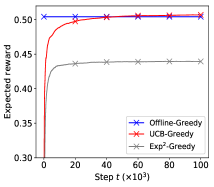
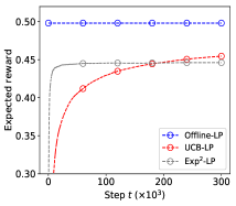
(a)                                (b)

Figure 1: Results on synthetic data with a single ad slot. (a) Expected reward of three approaches with Greedy oracle. (b) Expected reward of the same approaches with LP oracle.

Our results with Greedy oracle are reported in Figure 1a. We observe two major trends. First, UCB-Greedy learns quickly. In particular, its expected reward is around $0.5$ dollars in $30$k steps and exceeds $0.5$ dollars after $50$k steps. We note that UCB-Greedy slightly outperforms Offline-Greedy after $50$k steps. Indeed, since Greedy oracle is not guaranteed to return the optimal solution, it is possible to learn a better approximation online than offline. Second, Exp²-Greedy is consistently worse than UCB-Greedy and its expected reward is only $0.44$ dollars in $100$k steps. This shows that $n_{0}=500$ random exploration steps in Exp²-Greedy are less statistically efficient than more intelligent continuous exploration in UCB-Greedy.

The results with LP oracle are reported in Figure 1b. We observe similar trends to those in Figure 1a. One minor difference is that UCB-LP performs worse than Exp²-LP in the first $150$k steps. However, it outperforms Exp²-LP after $200$k steps and its expected reward approaches $0.45$ dollars in $300$k steps. The reason UCB-LP learns more slowly than UCB-Greedy is that the linear program in UCB-LP is not sensitive to small perturbations of model dynamics. That is, minor changes in the optimistic estimates of acceptance probabilities do not affect the output of the linear program. Therefore, UCB-LP explores all parameters of the model in the descending order of prices, which is inefficient. This is because higher prices are always preferred if the acceptance probabilities at all prices do not differ much. Only when the acceptance probabilities at higher prices become lower, UCB-LP explores other lower prices.

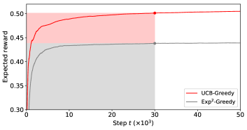
Figure 2: Illustration of publisher insights. The gray rectangle represents the revenue of Exp²-Greedy in $30\mathrm{k}$ steps, $0.438\times 30\mathrm{k}=13.14\mathrm{k}$ dollars. The red rectangle represents the difference in the revenues of UCB-Greedy and Exp²-Greedy in $30\mathrm{k}$ steps, $(0.501-0.438)\times 30\mathrm{k}=1.89\mathrm{k}$ dollars.

6.3 Publisher Insights

From the perspective of a publisher, our plots of the expected reward in the first $t$ steps can answer the following questions: (1) What is the revenue of a strategy up to step $t$? (2) What is the difference in revenues of strategies $A$ and $B$ up to step $t$?

The first question can be answered as follows. The revenue of a strategy up to step $t$ is equal to its expected reward up to step $t$ times $t$. In Figure 1a, for instance, the expected reward of Offline-Greedy in $100$k steps is $0.504$ dollars. Therefore, the revenue of Offline-Greedy in $100$k steps is $50.4$k dollars. The expected reward of UCB-Greedy in $100$k steps is $0.507$ dollars. Therefore, the revenue of UCB-Greedy in $100$k steps is $50.7$k dollars. By the same line of reasoning, the revenue of Exp²-Greedy in $100$k steps is $44$k dollars.

The second question can be answered as follows. The difference in revenues of strategies $A$ and $B$ up to step $t$ is equal to the difference of their expected rewards up to step $t$ times $t$. We illustrate this in Figure 2. The expected rewards of UCB-Greedy and Exp²-Greedy in $30$k steps are $0.501$ and $0.438$ dollars, respectively. Therefore, the difference in their expected rewards is $0.063$ dollars, and the difference in their revenues in $30$k steps is $1.89$k dollars. This increase in revenue is a result of the improved statistical efficiency of UCB-Greedy relative to Exp²-Greedy.

6.4 Real Data

6.4.1 Selling a Single Ad Slot

In this experiment, we show that our algorithm can learn to sell a single ad slot, whose dynamics is estimated from a real-world dataset.

We experiment with a real-world dataset of Real-Time Bidding (RTB) iPinYou [15]. This dataset contains information regarding bidding on ad slots, such as the identity of the ad slot, the winning advertiser, and the winning price. We treat each advertiser as an ad network. Perhaps surprisingly, the winning price of any advertiser on any ad slot does not change throughout the dataset. This is common in practice because many advertisers do not behave very strategically.

We estimate the valuations of ad networks as follows. Fix the ad slot. Let $n_{a}$ be the number of times that advertiser $a$ wins bidding and $v_{a}$ be its winning price, which does not change throughout the dataset. Then ad network $a$ accepts price $p$, independently of all other ad networks, with probability

$$\bar{w}(a,p)=\begin{cases}\displaystyle\mathbb{1}\{p\leq v_{a}\}\frac{n_{a}}{\sum_{a^{\prime}}n_{a^{\prime}}}\,,&p>0\,;\\ 1\,,&p=0\,;\end{cases}$$ (4)

where $n_{a}/\sum_{a^{\prime}}n_{a^{\prime}}$ is the frequency with which advertiser $a$ wins bids. Basically, $\bar{w}(a,p)$ is the empirical distribution of the acceptance probability of ad network $a$ when offered price $p$. We assume that the zero price is always accepted. This does not fundamentally change our problem and allows us to avoid boundary cases in our simulations.

We experiment with $20$ most active ad slots in the iPinYou RTB dataset, and refer to this subset of data as Active20. Specifically, there are nine advertisers bidding on these ad slots. The prices in the dataset are in $[0,300]$. We divide each price by $330$ in order to normalize all prices to $[0,1]$. As in Section 6.2, all algorithms operate on $11$ discrete price levels. The only major difference from Section 6.2 is that the valuations of ad networks are distributed according to (4).

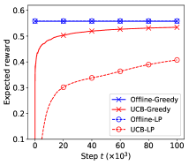
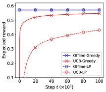
(a)                                (b)

Figure 3: Real-world problem with a single ad slot. (a) Expected reward up to step $t$ of Offline-X and UCB-X on the most active ad slot. (b) Average of the expected rewards of the same approaches over $10$ most active ad slots.

Our results on the most active ad slot in Active20 are reported in Figure 3a. We observe two major trends. First, Offline-X has the same performance irrespective of the oracle. The expected rewards of both Offline-Greedy and Offline-LP are $0.56$ dollars in $100$k steps, or equivalently $56$k dollars in revenue. Second, UCB-Greedy learns faster than UCB-LP. In particular, the expected reward of UCB-Greedy is $0.53$ dollars in $100$k steps, or equivalently $53$k dollars in revenue. The expected reward of UCB-LP is $0.41$ dollars in $100$k steps, or equivalently $41$k dollars in revenue. The difference in the revenues of two approaches in $100$k steps is $12$k dollars.

We also report the average performance of our algorithms on $10$ most active ad slots in Active20 in Figure 3b. These trends are extremely similar to those in Figure 3a. This experiment validates that our findings from Figure 3a are not limited to the most active ad slot, and that they apply to different ad slots.

6.4.2 Selling Multiple Ad Slots

Publishers often have different pages and sell hundreds of ad slots. To facilitate operations and speed up learning, one option is to learn a single selling strategy across multiple ad slots. In this experiment, we evaluate this option. In particular, if the acceptance probabilities of ad networks do not change much with the ad slots, learning of one common model is expected to lead to much faster learning of a near-optimal policy.

The acceptance probabilities of ad networks are estimated in the same way as Section 6.4.1. We consider the following model of interaction with multiple ad slots. Let $m$ be the number of ad slots. The ad slot at time $t$ is drawn uniformly at random from these $m$ ad slots. The publisher knows the identity of the ad slot at time $t$ and its goal is to maximize its reward, in expectation over the randomness in the choice of the ad slot at time $t$ and the behavior of ad networks. We propose two solutions to this problem. One is UCB-X that treats each ad slot separately and computes UCBs for all pairs of ad networks and prices in each ad slot. The other is Joint-UCB-X that treats all ad slots as a single slot, and computes UCBs for all pairs of ad networks and prices. Joint-UCB-X is expected to perform well if the acceptance probabilities of ad networks do not vary much across ad slots.

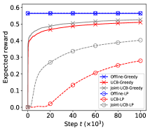
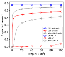
(a)                                (b)

Figure 4: Real-world problem with multiple ad slots. (a) Expected reward up to step $t$ of Offline-X, UCB-X, and Joint-UCB-X on five most active ad slots. (b) Expected reward of the same approaches on $20$ most active ad slots.

Our results on $m=5$ most active ad slots in Active20 are reported in Figure 4a. We observe two major trends. First, the expected rewards of both UCB-X and Joint-UCB-X improve over time. The expected reward of UCB-Greedy is $0.5$ dollars in $100$k steps, or equivalently $50$k dollars in revenue. The expected reward of Joint-UCB-Greedy is $0.53$ dollars in $100$k steps, or equivalently $53$k dollars in revenue. Second, Joint-UCB-X learns faster than UCB-X. In particular, the difference in the expected rewards of Joint-UCB-Greedy and UCB-Greedy is $0.03$ dollars in $100$k steps, or equivalently $3$k dollars in revenue. This highlights a common trade-off in learning. Although Joint-UCB-Greedy learns only an approximate model, this model is easier to learn in a finite time because it has $m$ times less parameters than UCB-Greedy. We observe the same trends with LP oracle.

Our results on all the ad slots in Active20 are reported in Figure 4b. These trends are similar to those in Figure 4a. We note that the benefits of Joint-UCB-Greedy and Joint-UCB-LP increase with $m$.

6.4.3 Selling to Aggregated Ad Networks

A common scenario is that publishers interact with third parties, which aggregate multiple ad networks. In this section, we study the impact of ad network aggregation on learning publisher revenue.

The third parties are modeled as follows. All ad networks are partitioned into $h$ groups, $G_{1},\ldots,G_{h}$. The values for $h$ will be specified later. When price $p$ is offered to group $G_{i}$, any ad network $a\in G_{i}$ accepts the offered price with probability $\bar{w}(a,p)$ in (4), independently of all other ad networks. If at least one $a\in G_{i}$ accepts, $G_{i}$ accepts. From the point of view of the publisher and our algorithms, each group is treated as an ad network.

Learning with Aggregated Ad Networks.   We first show that our algorithm can learn to sell to aggregated ad networks. We also show that LP oracle leads to faster learning than Greedy oracle when the dynamics of selling is more complicated.

We set $h=2$ and evaluate Offline-X and UCB-X on the most active ad slot in Active20 dataset under two settings. In the first experiment, we fix six ad networks in $G_{1}$ and put the remaining three ad networks in $G_{2}$. In the second experiment, we put six random ad networks in $G_{1}$ and the remaining three ad networks in $G_{2}$. This experiment is repeated with $10$ random partitions.

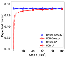
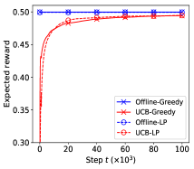
(a)                                (b)

Figure 5: Real-world problem with aggregated ad networks. (a) Expected reward up to step $t$ of Offline-X and UCB-X over the fixed partition of the most active ad slot. (b) Average of the expected rewards of the same approaches over $10$ random partitions.

The results of the first experiment are shown in Figure 5a. We observe one major trend. The expected reward of UCB-X converges to that of the best approximation in hindsight irrespective of the oracle. For example, the expected reward of Offline-X is around $0.48$ dollars in $100$k steps, or equivalently $48$k dollars in revenue. The expected reward of UCB-X reaches almost $0.478$ dollars in $100$k steps, or equivalently $47.8$k dollars in revenue. The difference in revenues is merely $200$ dollars, which indicates that UCB-X can learn a very good approximation in this experiment.

The results of the second experiment are shown in Figure 5b. We make two additional observations. First, the trends are very similar to those in Figure 5a. This shows that our algorithm UCB-X does not overfit to a specific group of ad networks. Second, algorithms with LP oracle learn slightly faster than those with Greedy oracle. For example, the expected reward of UCB-Greedy and UCB-LP are respectively $0.491$ and $0.493$ dollars in $60$k steps. The difference of the expected rewards is $0.002$ dollars in $60$k steps, or equivalently $120$ dollars in revenue.

Publisher revenue with Aggregated Ad Networks.   Finally, we study the impact of ad network aggregation on the expected revenue of publisher.

Again, we evaluate Offline-X and UCB-X on the most active ad slot in Active20 dataset but under three different configurations:

1. Configuration 1: $h=2$ with group sizes of six and three.

2. Configuration 2: $h=3$ with group sizes of four, four and one.

3. Configuration 3: $h=9$ where all group sizes are one.

These configurations represent different degrees of ad network aggregation. In all the configurations, the ad networks are partitioned in a uniformly random fashion. Each configuration is repeated for $10$ times.

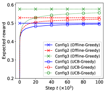
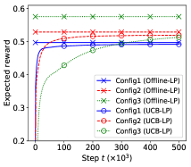
(a)                                (b)

Figure 6: Impact of three configurations of aggregated ad networks on expected revenues. (a) Publisher expected reward up to step $t$ for oracle Greedy. (b) Publisher expected reward up to step $t$ for oracle LP.

The results of oracles Greedy and LP are respectively reported in Figure 6a and Figure 6b. We observe the similar results to the previous experiment that our algorithms can learn to sell under all the configurations of ad network aggregations. Moreover, we observe two additional interesting trends.

First, less aggregation of ad networks results in higher expected reward. Take the oracle Greedy as example. As shown in Figure 6a, the expected rewards of Offline-Greedy and UCB-Greedy under Configuration 3 are respectively $0.576$ and $0.556$ dollars in $100$k steps. They are both higher than the expected rewards acquired from other configurations where ad networks aggregate into groups. One explanation is that less aggregation of ad networks allows the publisher to better customize prices to ad networks, and hence the expected reward is higher.

Second, less aggregation of ad networks requires longer time to find the optimal solution, especially for the algorithm UCB-LP. To illustrate this phenomenon, we run all algorithms with oracle LP for more steps ($t=500$k). As shown in Figure 6b, the expected reward of UCB-LP reaches $0.513$ dollars in $500$k steps when there are nine individual ad networks (Configuration 3). It exceeds the expected reward of $0.492$ dollars in the case of two aggreated groups (Configuration 1) and is close to $0.519$ dollars of three groups (Configuration 2). With less aggregation, although our algorithm statistically should be able to collect more responses per waterfall run, it needs to learn the behavior of more groups.

7 Related Work

Our work is at the intersection of online advertising and online learning with partial feedback.

The problem of waterfall optimization was studied before under the name of “sequential posted price mechanisms” [7, 6, 1, 4, 10]. In [7, 6, 1], the acceptance probabilities of ad networks are assumed to be known by the publisher. [4, 10] study the waterfall optimization problem in an online setting, under the assumption that all ad networks have the same acceptance probabilities. We do not make any of these assumptions.

Our work is a generalization of online learning to rank in the cascade model [11, 12]. More specifically, cascading bandits can be viewed as waterfall bandits when $Q=\{1\}$. This seemingly minor change has major implications. For instance, when $Q=\{1\}$, the optimal solution in (2) can be computed greedily. In our case, no polynomial-time algorithm is known for solving (2). From the learning point of view, we learn $KM$ statistics. In cascading bandits, only $K$ statistics are learned because $M=|Q|=1$.

Our problem is a form of partial monitoring [5, 2], which is a harder class of learning problems than multi-armed bandits. The general algorithms in partial monitoring cannot solve our problem computationally efficiently because their computational cost is $\Omega(|\mathcal{A}|)$, where $|\mathcal{A}|$ is exponential in the number of ad networks.

Our setting is also reminiscent of stochastic combinatorial semi-bandits [9, 8, 13, 18], which can be solved statistically efficiently by UCB-like algorithms. The difference is that our feedback is less than semi-bandit. In particular, if an ad network accepts an offer, the learning agent does not learn if any of the subsequent ad networks would have accepted their offered prices. In combinatorial semi-bandits, all of these events are assumed to be observed. Therefore, our problem cannot be solved as a combinatorial semi-bandit.

8 Conclusions

For the waterfall, we propose the algorithm ${\tt WaterfallUCB1}$, a computationally and sample efficient online algorithm for learning to price, which maximizes the expected revenue of the publisher. We derive a sublinear upper bound on the $n$-step regret of ${\tt WaterfallUCB1}$. Note that ${\tt WaterfallUCB1}$ solves a general problem of learning to maximize (2) from partial feedback. Therefore, although our main focus is online advertising, the algorithm may have other applications, especially in learning to price.

We evaluate ${\tt WaterfallUCB1}$ on both synthetic and real-world data, and show that it quickly learns competitive strategies to the best approximations in hindsight. In addition, we investigate multiple real-world scenarios that are of a particular interest of publishers. We show that ${\tt WaterfallUCB1}$ can learn to sell in these scenarios and it does not overfit.

We leave open several questions of interest. For instance, note that the update of statistics in ${\tt WaterfallUCB1}$ can be easily modified to leverage the following two monotonicity properties. When ad network $a$ accepts price $p$, it would have accepted any lower price $p^{\prime}<p$. Similarly, when ad network $a$ does not accept price $p$, it would have not accepted any higher price $p^{\prime}>p$. Roughly speaking, this would make ${\tt WaterfallUCB1}$ more statistically efficient. However, it is non-trivial to prove that this would result in a better regret bound than that in Section 5. We leave these for future work.

Appendix A Appendix: Proof of Theorem 1

We first prove that the function $f(A,u)$ is monotone in the weight function $u$, for any fixed action $A$.

[] Consider $\bar{w},\bar{v}\in[0,1]^{[K]\times Q}$ such that for all $i\in[K],j\in Q$, $\bar{w}(i,j)\leq\bar{v}(i,j)$. If the items of action $A$ are sorted in descending order of prices, then

$$f(A,\bar{w})\leq f(A,\bar{v})$$ (5)

Proof.

We prove Lemma 5 based on the mathematical induction on $K$, the number of ad networks.

Induction base: We first prove that equation 5 holds for the case with $K=1$. Notice that for $K=1$,

$$f(A,\bar{w})=p_{1}\bar{w}(a_{1},p_{1})\leq p_{1}\bar{v}(a_{1},p_{1})=f(A,\bar{v})$$ (6)

Induction step: For any integer $m\geq 1$, we then prove that if equation 5 holds for $K=m$, then it also holds for $K=m+1$. Recall that for $K=m+1$, $A=\left((a_{1},p_{1}),\ldots,(a_{m+1},p_{m+1})\right)$. To simplify the exposition, we also define the term $\tilde{A}=\left((a_{2},p_{2}),\ldots,(a_{m+1},p_{m+1})\right)$. Notice that

$$f(A,\bar{w})= \bar{w}(a_{1},p_{1})p_{1}+(1-\bar{w}(a_{1},p_{1}))f(\tilde{A},\bar{w})$$

$$\stackrel{{\scriptstyle(a)}}{{\leq}} \bar{w}(a_{1},p_{1})p_{1}+(1-\bar{w}(a_{1},p_{1}))f(\tilde{A},\bar{v})$$

where $(a)$ follows the induction hypothesis. Moreover, since $f(\tilde{A},\bar{v})$ is the expected revenue of $\tilde{A}$, $f(\tilde{A},\bar{v})\leq p_{2}\leq p_{1}$. Therefore,

$$0\leq(p_{1}-f(\tilde{A},\bar{v}))(\bar{v}(a_{1},p_{1})-\bar{w}(a_{1},p_{1}))$$ (7)

which implies

$$\,\bar{w}(a_{1},p_{1})p_{1}+(1-\bar{w}(a_{1},p_{1}))f(\tilde{A},\bar{v})\leq\,\bar{v}(a_{1},p_{1})p_{1}+(1-\bar{v}(a_{1},p_{1}))f(\tilde{A},\bar{v})=\,f(A,\bar{v})$$

As a result, $f(A,\bar{w})\leq f(A,\bar{v})$. ∎

We now prove Theorem 1. First, we define the “bad event” $\mathcal{E}_{t}$ at time $t$ as the event that at least one $\bar{w}(e)$ is outside its confidence interval at time $t$,

$$\mathcal{E}_{t}=\{\exists e\in E\;s.t.\;|\bar{w}(e)-\hat{w}_{T_{t-1}(e)}(e)|>c_{t-1,T_{t-1}(e)}\}\,.$$ (8)

Notice that $\bar{\mathcal{E}}_{t}$, the complement of $\mathcal{E}_{t}$, is considered as the “good event” at time $t$. Similar to [11], we define the event $G_{e,t}$ as the event that item $e=(a,p)$ is “observed” at time $t$ (i.e. ad network $a$ is called and offered price $p$ at time $t$):

$$G_{e,t}= \{\exists 1\leq k\leq K\ni\;d_{t,k}=e,B_{t}\geq k\}$$ (9)

where $d_{t,i}=(a_{t,i},p_{t,i})$. In addition, we define $\mathbb{E}_{t}[\cdot]=\mathbb{E}[\cdot|\mathbb{H}_{t}]$ where $\mathbb{H}_{t}$ is the history of all actions and feedbacks until time $t-1$ plus the action $A_{t}$, which is determined by $\mathbb{H}_{t}$ under Algorithm 3. The following lemma bounds the per-step scaled regret $R_{t}^{\gamma}=\gamma f(A^{*},\bar{w})-f(A_{t},\bar{w})$ under the “good event” $\bar{\mathcal{E}}_{t}$:

Proof.

Conditioning on the event $\bar{\mathcal{E}}_{t}$, we have $\bar{w}\leq U_{t}$. Lemma 5 states that $\bar{w}\leq U_{t}$ implies $f(A,\bar{w})\leq f(A,U_{t})$. Then we have the following bound on $R_{t}^{\gamma}$:

$$R_{t}^{\gamma}\stackrel{{\scriptstyle(a)}}{{=}} \gamma f(A^{*},\bar{w})-f(A_{t},\bar{w})$$

$$\stackrel{{\scriptstyle(b)}}{{\leq}} \gamma f(A^{*},U_{t})-f(A_{t},\bar{w})$$

$$\leq \gamma\max_{A}f(A,U_{t})-f(A_{t},\bar{w})$$

$$\stackrel{{\scriptstyle(c)}}{{\leq}} f(A_{t},U_{t})-f(A_{t},\bar{w}),$$ (10)

where (a) follows from the definition of $R_{t}^{\gamma}$, (b) follows from Lemma 5, and (c) follows from the fact that $A_{t}$ is computed from a $\gamma$-approximation algorithm.

To simplify the exposition, in the rest of this proof, we use $\bar{w}_{i}$ and $U_{i}$ to respectively denote $\bar{w}(a_{t,i},p_{t,i})$ and $U_{t}(a_{t,i},p_{t,i})$, and use $p_{i}$ to denote $p_{t,i}$. Then we have

$$R_{t}^{\gamma}\stackrel{{\scriptstyle(a)}}{{\leq}} \,\sum_{i=1}^{K}\left[\prod_{j<i}[1-U_{j}]\right]U_{i}p_{i}-\sum_{i=1}^{K}\left[\prod_{j<i}[1-\bar{w}_{j}]\right]\bar{w}_{i}p_{i}$$

$$\stackrel{{\scriptstyle(b)}}{{\leq}} \,\sum_{i=1}^{K}\left[\prod_{j<i}[1-\bar{w}_{j}]\right]U_{i}p_{i}-\sum_{i=1}^{K}\left[\prod_{j<i}[1-\bar{w}_{j}]\right]\bar{w}_{i}p_{i}$$

$$\stackrel{{\scriptstyle(c)}}{{=}} \,\sum_{i=1}^{K}\left[\prod_{j<i}[1-\bar{w}_{j}]\right]\left(U_{i}-\bar{w}_{i}\right)p_{i}$$

$$\stackrel{{\scriptstyle(d)}}{{\leq}} \,\sum_{i=1}^{K}\left[\prod_{j<i}[1-\bar{w}_{j}]\right]\left(U_{i}-\bar{w}_{i}\right),$$ (11)

where (b) follows from $\bar{w}_{i}\leq U_{i}$ for all $i$ under event $\bar{\mathcal{E}}_{t}$, and (d) follows from $0<p_{i}\leq 1$ for all $i$. Notice that $U_{i}-\bar{w}_{i}$ is the “item-wise” difference between the upper confidence and the mean, and $\prod_{j<i}[1-\bar{w}_{j}]$ is the conditional probability that the $i$th ad network will be called. We have

$$\prod_{j<i}[1-\bar{w}_{j}]=\mathbb{E}_{t}\left\{\mathbb{1}\{G_{d_{t,i},t}\}\right\}\,.$$ (12)

From (11), we have

$$R^{\gamma}_{t}\leq\sum_{i=1}^{K}\mathbb{E}_{t}\left\{\mathbb{1}\{G_{d_{t,i},t}\}\right\}\phi_{(a_{t,i},p_{t,i}),t}\,.$$ (13)

∎

We use Lemma 5 to bound $R^{\gamma}(n)$ as follows. Notice that $R^{\gamma}(n)=\mathbb{E}[\sum_{t=1}^{n}\mathbb{1}\{\mathcal{E}_{t}\}R^{\gamma}_{t}]+\mathbb{E}[\sum_{t=1}^{n}\mathbb{1}\{\bar{\mathcal{E}}_{t}\}R^{\gamma}_{t}]$. We use $e$ to refer to an item in $E$. As discussed, all prices are less or equal to 1; so, $0\leq f(A,w)\leq 1$. Hence, we have $R^{\gamma}_{t}\leq\gamma$. As a result,

$$\mathbb{E}[\sum_{t=1}^{n}\mathbb{1}\{\mathcal{E}_{t}\}R^{\gamma}_{t}]\leq\gamma\mathbb{E}[\sum_{t=1}^{n}\mathbb{1}\{\mathcal{E}_{t}\}]$$

$$\leq \gamma\sum_{e\in E}\sum_{t=1}^{n}\sum_{s=1}^{t}\mathbb{P}(|\bar{w}(e)-\hat{w}_{s}(e)|\geq c_{t,s})$$

$$\stackrel{{\scriptstyle(a)}}{{\leq}} 2\gamma\sum_{e\in E}\sum_{t=1}^{n}\sum_{s=1}^{t}\exp(-3\log t)$$

$$\leq 2\gamma\sum_{e\in E}\sum_{t=1}^{n}t^{-2}\leq\gamma\frac{\pi^{2}}{3}|E|=\gamma\frac{\pi^{2}}{3}MK$$

In the above derivation, $(a)$ follows Hoeffding’s inequality. Notice that for all $e\in E$ and $t\leq n$, we have (1) $\phi_{e,t}\leq 2c_{t-1,T_{t-1}(e)}$ under event $\bar{\mathcal{E}}_{t}$, (2) $c_{t-1,T_{t-1}(e)}\leq c_{n,T_{t-1}(e)}$. Based on Lemma 5, we have

$$\mathbb{E}\left[\sum_{t=1}^{n}\mathbb{1}\{\bar{\mathcal{E}}_{t}\}R^{\gamma}_{t}\right]\leq\sum_{e\in E}\mathbb{E}\left[\sum_{t=1}^{n}\mathbb{1}\{\bar{\mathcal{E}}_{t},G_{e,t}\}\phi_{e,t}\right]$$

$$\leq \;2\sum_{e\in E}\mathbb{E}\left[\sum_{t=1}^{n}\mathbb{1}\{\bar{\mathcal{E}}_{t},G_{e,t}\}c_{t-1,T_{t-1}(e)}\right]\leq\;2\sqrt{1.5\log n}\sum_{e\in E}\mathbb{E}\left[\sum_{t=1}^{n}\mathbb{1}\{\bar{\mathcal{E}}_{t},G_{e,t}\}\sqrt{\frac{1}{T_{t-1}(e)}}\right]$$

Notice that $T_{t-1}(e)\leq n$ and once $e$ is observed, $T_{t}(e)$ is increased by $1$, thus we have

$$\mathbb{E}[\sum_{t=1}^{n}\mathbb{1}\{\bar{\mathcal{E}}_{t},G_{e,t}\}\sqrt{\frac{1}{T_{t-1}(e)}}]\leq\sum_{t=1}^{n}\frac{1}{\sqrt{t}}\leq 1+\int_{1}^{n}\frac{1}{\sqrt{t}}dt\leq 2\sqrt{n}-1<2\sqrt{n}$$

Recall that $|E|=MK$, we have

$$\mathbb{E}[\sum_{t=1}^{n}\mathbb{1}\{\bar{\mathcal{E}}_{t}\}R^{\gamma}_{t}]\leq 4MK\sqrt{1.5n\log n}$$

This concludes the proof for Theorem 1.

References

- [1] Marek Adamczyk, Allan Borodin, Diodato Ferraioli, Bart De Keijzer, and Stefano Leonardi. Sequential posted-price mechanisms with correlated valuations. ACM Transactions on Economics and Computation (TEAC), 5(4):22, 2017.
- [2] Rajeev Agrawal, Demosthenis Teneketzis, and Venkatachalam Anantharam. Asymptotically efficient adaptive allocation schemes for controlled i.i.d. processes: Finite parameter space. IEEE Transactions on Automatic Control, 34(3):258–267, 1989.
- [3] Peter Auer, Nicolo Cesa-Bianchi, and Paul Fischer. Finite-time analysis of the multiarmed bandit problem. Machine Learning, 47:235–256, 2002.
- [4] Moshe Babaioff, Shaddin Dughmi, Robert Kleinberg, and Aleksandrs Slivkins. Dynamic pricing with limited supply. ACM Transactions on Economics and Computation (TEAC), 3(1):4, 2015.
- [5] Gabor Bartok, Navid Zolghadr, and Csaba Szepesvari. An adaptive algorithm for finite stochastic partial monitoring. In Proceedings of the 29th International Conference on Machine Learning, 2012.
- [6] Tanmoy Chakraborty, Eyal Even-Dar, Sudipto Guha, Yishay Mansour, and S Muthukrishnan. Approximation schemes for sequential posted pricing in multi-unit auctions. In WINE, pages 158–169. Springer, 2010.
- [7] Shuchi Chawla, Jason D Hartline, David L Malec, and Balasubramanian Sivan. Multi-parameter mechanism design and sequential posted pricing. In Proceedings of the forty-second ACM symposium on Theory of computing, pages 311–320. ACM, 2010.
- [8] Wei Chen, Yajun Wang, and Yang Yuan. Combinatorial multi-armed bandit and its extension to probabilistically triggered arms. CoRR, abs/1407.8339, 2014.
- [9] Yi Gai, Bhaskar Krishnamachari, and Rahul Jain. Combinatorial network optimization with unknown variables: Multi-armed bandits with linear rewards and individual observations. IEEE/ACM Transactions on Networking, 20(5):1466–1478, 2012.
- [10] Robert Kleinberg and Tom Leighton. The value of knowing a demand curve: Bounds on regret for online posted-price auctions. In Foundations of Computer Science, 2003. Proceedings. 44th Annual IEEE Symposium on, pages 594–605. IEEE, 2003.
- [11] Branislav Kveton, Csaba Szepesvari, Zheng Wen, and Azin Ashkan. Cascading bandits: Learning to rank in the cascade model. In Proceedings of the 32nd International Conference on Machine Learning, 2015.
- [12] Branislav Kveton, Zheng Wen, Azin Ashkan, and Csaba Szepesvari. Combinatorial cascading bandits. In Advances in Neural Information Processing Systems 28, pages 1450–1458, 2015.
- [13] Branislav Kveton, Zheng Wen, Azin Ashkan, and Csaba Szepesvari. Tight regret bounds for stochastic combinatorial semi-bandits. In Proceedings of the 18th International Conference on Artificial Intelligence and Statistics, 2015.
- [14] T. L. Lai and Herbert Robbins. Asymptotically efficient adaptive allocation rules. Advances in Applied Mathematics, 6(1):4–22, 1985.
- [15] Hairen Liao, Lingxiao Peng, Zhenchuan Liu, and Xuehua Shen. ipinyou global rtb bidding algorithm competition dataset. In Proceedings of the Eighth International Workshop on Data Mining for Online Advertising, pages 1–6. ACM, 2014.
- [16] Richard S Sutton and Andrew G Barto. Reinforcement learning: An introduction, volume 1. MIT press Cambridge, 1998.
- [17] Satya Vinnakota. In your waterfall - how publishers monetise their ad inventory, June 2017.
- [18] Zheng Wen, Branislav Kveton, and Azin Ashkan. Efficient learning in large-scale combinatorial semi-bandits. In Proceedings of the 32nd International Conference on Machine Learning, 2015.
- [19] Maciej Zawadzinski. What is waterfalling and how does it work?, September 2016.