Data-Driven Neuron Allocation for Scale Aggregation Networks

Abstract

Successful visual recognition networks benefit from aggregating information spanning from a wide range of scales. Previous research has investigated information fusion of connected layers or multiple branches in a block, seeking to strengthen the power of multi-scale representations. Despite their great successes, existing practices often allocate the neurons for each scale manually, and keep the same ratio in all aggregation blocks of an entire network, rendering suboptimal performance. In this paper, we propose to learn the neuron allocation for aggregating multi-scale information in different building blocks of a deep network. The most informative output neurons in each block are preserved while others are discarded, and thus neurons for multiple scales are competitively and adaptively allocated. Our scale aggregation network (ScaleNet) is constructed by repeating a scale aggregation (SA) block that concatenates feature maps at a wide range of scales. Feature maps for each scale are generated by a stack of downsampling, convolution and upsampling operations. The data-driven neuron allocation and SA block achieve strong representational power at the cost of considerably low computational complexity. The proposed ScaleNet, by replacing all $3\times 3$ convolutions in ResNet with our SA blocks, achieves better performance than ResNet and its outstanding variants like ResNeXt and SE-ResNet, in the same computational complexity. On ImageNet classification, ScaleNets absolutely reduce the top-1 error rate of ResNets by 1.12 (101 layers) and 1.82 (50 layers). On COCO object detection, ScaleNets absolutely improve the mmAP with backbone of ResNets by 3.6 (101 layers) and 4.6 (50 layers) on Faster RCNN, respectively. Code and models are released at https://github.com/Eli-YiLi/ScaleNet.

1 Introduction

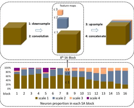
Figure 1: Illustration of the data-driven neuron allocation for the scale aggregation (SA) block. The proportion of output neurons (or channels) of different scales in an SA block is learned, and thus adaptively changes across layers in a network.

Deep convolutional neural networks (CNNs) have been successfully applied to a wide range of computer vision tasks, such as image classification [18], object detection [25], and semantic segmentation [22], due to their powerful end-to-end learnable representations. From bottom to top, the layers of CNNs have larger receptive fields with coarser scales, and their corresponding representations become more semantic. Aggregating context information from multiple scales has been proved to be effective for improving accuracy [32, 9, 13, 20, 6, 3, 16, 28, 4]. Small scale representations encode local structures such as textures, corners and edges, and are useful for localization, while coarse scale representations encode global contexts such as object categories, object interaction and scene, and thus clarify local confusion.

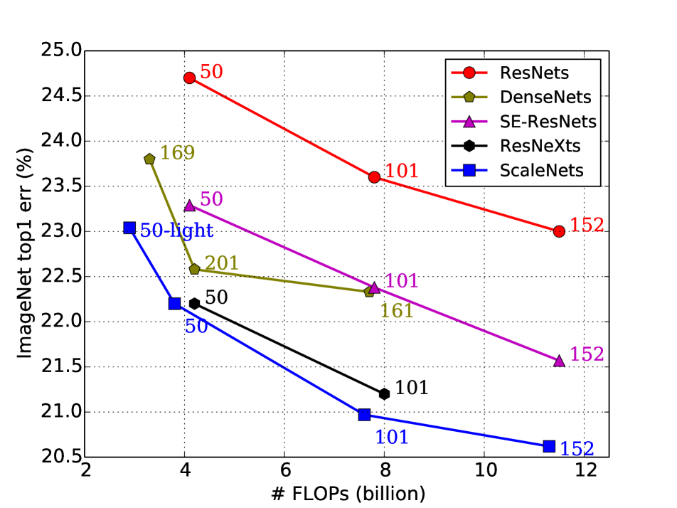
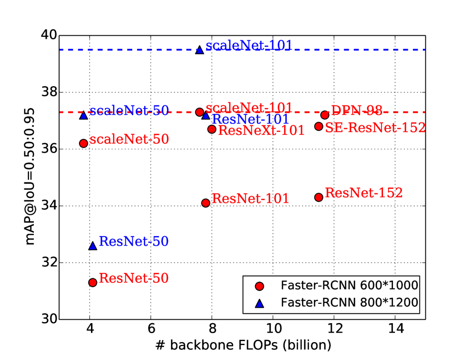
Figure 2: Comparison of the ScaleNets and modern architectures’ top-1 error rates (single-crop testing) on the ImageNet validation dataset (left) and mAP on MS COCO mini-validation set (right) as a function of FLOPs during testing. ScaleNet-50-light indicates a light ScaleNet which is also constructed from ResNet-50. Architectures are given in the Appendix D.

There exist many previous attempts to fuse multi-scale representations by designing network architecture. They aggregate multi-scale representations of connected layers with different depths [32, 9, 13, 20, 6, 3, 16, 12, 26] or multiple branches in a block with different convolutional kernel sizes [28, 4]. The proportion of multi-scale representations for in each aggregation block is manually set in a trial-and-error process and kept the same in the entire network. Ideally, the most efficient architecture design of multi-scale information aggregation is adaptive. The proportion of neurons for each scale is determinate according to the importance of the scale in gathering context. Such proportion should also be adaptive to the stage in the network. Bottom layers may prefer fine scales and top layers may prefer coarse scales.

In this paper, we propose a novel data-driven neuron allocation method for multi-scale aggregation, which automatically learns the neuron proportion for each scale in all aggregation blocks of one network. We model the neuron allocation as one network optimization problem under FLOPs constraints which is solved by SGD and back projection. Concretely, we train one seed network with abundant output neurons for all scales using SGD, and then project the trained network into one feasible network that meets the constraints by selecting the top most informative output neurons amongst all scales. In this way, the neuron allocation for multi-scale representations is learnable and tailored for the network architecture.

To effectively extract and utilize multi-scale information, we present a simple yet effective Scale Aggregation (SA) block to strengthen the multi-scale representational power of CNNs. Instead of generating multi-scale representations with connected layers of different depths or multi-branch different kernel sizes as done in [28, 9, 32, 9, 13, 20, 6, 3, 16], an SA block explicitly downsamples the input feature maps with a group of factors to small sizes, and then independently conducts convolution, resulting in representations in different scales. Finally, the SA block upsamples the multi-scale representations back to the same resolution as that of the input feature maps and concatenate them in channel dimension together. We use SA blocks to replace all $3\times 3$ convolutions in ResNets to form ScaleNets. Thanks to downsampling in each SA block, ScaleNets are very efficient by decreasing the sampling density in the spatial domain, which is independent yet complementary to network acceleration approaches in the channel domain. he proposed SA block is more computationally efficient and can capture a larger scale (or receptive field) range as shown in Figure  6, compared with previous multi-scale architecture.

We apply the proposed technique of data-driven neuron allocation to the SA block to form a learnable SA block. To demonstrate the effectiveness of the learnable SA block, we use learnable SA blocks to replace all $3\times 3$ convolutions in ResNet to form a novel architecture called ScaleNet. The proposed ScaleNet outperforms ResNet and its outstanding variants such as ResNeXt [31] and SE-ResNet [11], as well as recent popular architectures such as DenseNet [13], with impressive margins on image classification and object detection while keeping the same computational complexity as shown in Figure 2. Specifically, ScaleNet-50 and ScaleNet-101 absolutely reduces the top-1 error rate of ResNet-101 and ResNet-50 by 1.12% and 1.82% on ImageNet respectively. Benefiting from the strong multi-scale representation power of learnable SA blocks, ScaleNets are considerably effective on object detection. The Faster-RCNN [25] with backbone ScaleNet-101 and ScaleNet-50 absolutely improve the mmAP of those with ResNet-101 and ResNet-50 by 3.6 and 4.6 on MS COCO.

2 Related Work

Multi-scale representation aggregation has been studied for a long time. It can be categorized into shortcut connection approaches and multi-branch approaches.

Shortcut connection approaches. Connected layers with different depths usually have different receptive fields, and thus multi-scale representations. Shortcut connections between layers not only maximize information flow to avoid vanishing gradient, but also strengthen multi-scale representation power of CNNs. ResNet [9], DenseNet [13], and Highway Network [27] fuse multi-scale information by identity shortcut connections or gating function based ones. Deep layer aggregation [32] further extends shortcut connection with trees that cross stages. In object detection, FPN [20] fuses coarse scale representations to fine scale ones from top to down in one detector’s header [20]. ASIF [6] merges multi-scale representations from $4$ layers both from top to down and from down to top. HyperNet [16] and ION [3] concatenate multi-scale features from different layers to make prediction. All the shortcut connection approaches focus on reusing fine scale representations from preceding layers or coarse scale ones from subsequent layers. Due to limited connection patterns between layers, the scale (or receptive filed) range is limited. Instead, the proposed approach generates a wide range scale of representations with a group of downsampling factors itself in each SA block. Moreover, it is a general and standard module which can replace any convolutional layer of existing networks, and be effectively used in various tasks such as image classification and object detection as validated in our experiments.

Multi-branch approaches. The most influential multi-branch network is GoogleNet [28], where each branch is designed with different depths and convolutional kernel sizes. Its branches have varied receptive fields and multi-scale representations. Similar multi-branch network is designed for crowd counting in [4]. Different from previous multi-branch approaches, the proposed SA block generates multi-scale representations by downsampling the input feature maps by different factors to expand the scale of representations. Again, it can generate representations with wider scale range than  [28, 4]. Downsampling is also used in the context module of PSPNet [34] and ParseNet [24]. However, the context module is only used in the network header while the proposed SA block is used in the whole backbone and thus more general. Moreover, the neuron proportion for each scale is manually set and fixed in the context module while automatically learned and different from one SA block to another in one network.

Our data-driven neuron allocation method is also related to network pruning methods [8, 2, 30, 19] or network architecture search methods [35, 29]. However, our data-driven neuron allocation method targets at multi-scale representation aggregation but not the whole architecture design. It learns the neuron proportion for scales in each SA block separately. In this way, the neuron allocation problem is greatly simplified, and easily optimized.

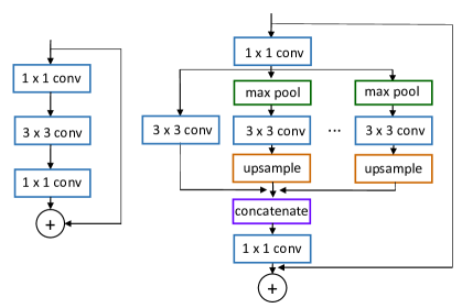
Figure 3: Illustration of the SA block. The left shows the original residual block, and the right shows the module after replacing the $3\times 3$ convolution by the SA block.

3 ScaleNets

3.1 Scale Aggregation Block

The proposed scale aggregation block is a standard computational module which readily replaces any given transformation $\mathbf{Y}=\mathbf{T}(\mathbf{X})$, where $\mathbf{X}\in\mathbb{R}^{H\times W\times C}$, $\mathbf{Y}\in\mathbb{R}^{H\times W\times C_{o}}$ with $C$ and $C_{o}$ being the input and output channel number respectively. $\mathbf{T}$ is any operator such as a convolution layer or a series of convolution layers. Assume we have $L$ scales. Each scale $l$ is generated by sequentially conducting a downsampling $\mathbf{D}_{l}$, a transformation $\mathbf{T}_{l}$ and an unsampling operator $\mathbf{U}_{l}$:

$$\mathbf{X}^{{}^{\prime}}_{l}=\mathbf{D}_{l}(\mathbf{X}),$$ (1)

$$\mathbf{Y}^{{}^{\prime}}_{l}=\mathbf{T}_{l}(\mathbf{X}^{{}^{\prime}}_{l}),$$ (2)

$$\mathbf{Y}_{l}=\mathbf{U}_{l}(\mathbf{Y}^{{}^{\prime}}_{l}),$$ (3)

where $\mathbf{X}^{{}^{\prime}}_{l}\in\mathbb{R}^{H_{l}\times W_{l}\times C}$, $\mathbf{Y}^{{}^{\prime}}_{l}\in\mathbb{R}^{H_{l}\times W_{l}\times C_{l}}$, and $\mathbf{Y}_{l}\in\mathbb{R}^{H\times W\times C_{l}}$. Notably, $\mathbf{T}_{l}$ has the similar structure as $\mathbf{T}$. Substitute Equation (1) and (2) into Equation (3), and concatenate all $L$ scales together, getting

$$\mathbf{Y}^{{}^{\prime}}=\|^{L}_{1}\mathbf{U}_{l}(\mathbf{T}_{l}(\mathbf{D}_{l}(\mathbf{X}))),$$ (4)

where $\|$ indicates concatenating feature maps along the channel dimension, and $\mathbf{Y}^{{}^{\prime}}\in\mathbb{R}^{H\times W\times\sum^{L}_{1}C_{l}}$ is the final output feature maps of the scale aggregation block.

In our implementation, the downsampling $\mathbf{D}_{l}$ with factor $s$ is implemented by a max pool layer with $s\times s$ kernel size and $s$ stride. The upsampling $\mathbf{U}_{l}$ is implemented by resizing with the nearest neighbor interpolation.

3.2 Data-Driven Neuron Allocation

There exist $L$ scales in each SA block. Different scales should play different roles in blocks with different depths. Therefore, simply allocating the output neuron proportion of scales equally would lead to suboptimal performance. Our core idea is to identify the importance of each output neuron, and then prune the unimportant neurons while preserving the important ones. For each output neuron, we employ its corresponding scale weight ($\gamma$) of its subsequent BatchNorm [15] layer to evaluate its importance. The underlying reason is that $\gamma$ is positively correlated with the output confidence of its corresponding neuron.

Let $K$, $O_{k}$ ($1\leq k\leq K$), and $O_{kl}$ ($1\leq k\leq K$ and $1\leq l\leq L$) denote the total SA block index of the target network, the computational complexity budget of the $k^{th}$ SA block, and the computational complexity of one output neuron at scale $l$ in the $k^{th}$ block respectively. We target at optimally allocating neurons for each scale in the $k^{th}$ SA block with the budget $O_{k}$. Formally, we have

$$\min\limits_{\theta}\ F(\theta),\ \text{s.t.}\ \forall k,\sum_{1\leq n\leq N_{k}}O_{kl(\theta_{kn})}\leq O_{k},$$ (5)

where $F(\theta)$ is the loss function of the whole network with $\theta$ being the learnable weights of the network, and $\theta_{kn}$ being the weight of $n^{th}$ output neuron in the $k^{th}$ SA block. $l(\cdot)$ indicates the scale index, and $N_{k}$ is the total number of output neurons in the $k^{th}$ SA block.

We optimize the objective function (5) by SGD with projection. We first optimize $F(\theta)$, getting $\theta^{t}$, we then project $\theta_{t}$ back to the feasible domain defined by constraints for each SA block $k$ by optimizing

$$\begin{split}\min\limits_{\theta}&\sum\limits_{n}\mathinner{\!\left\lvert\mathbf{V}(\theta_{kn})-\mathbf{V}(\theta_{kn}^{t})\right\rvert}\\ &\text{s.t.}\ \sum_{1\leq n\leq N_{k}}O_{kl(\theta_{kn})}\leq O_{k},\end{split}$$ (6)

where $\mathbf{V}(\theta_{kn})$ indicates the importance of the $n^{th}$ neuron in the $k^{th}$ SA block. It is defined to be the scale weight which corresponds to the target channel $(k,n)$ in its subsequent BatchNorm layer as done in [8]. The more important and of less computational complexity the neuron is, the more likely it should be preserved. Equation (6) is greedily solved by selecting neurons with top biggest $\mathbf{V}(\theta_{kn})/O_{kl(\theta_{kn})}^{b}$ in the $k^{th}$ SA block. Note that $b$ is an exponential balance factor of computational complexity. We found $b=0$ achieves good results in our experiments.

Algorithm 1 lists the procedure of neuron allocation. First, we set a seed network by setting $C$ neurons for each scale (i.e., $N_{k}=CL$). Second, we train the seed network till convergence. Third, we select the top most important neurons in SA blocks by solving Equation( 6), and get a new network. Finally, we retrain the new network from scratch.

Algorithm 1 Data-driven neuron allocation

Initialize a seed network by setting $N_{k}=LC$
Train the seed network till convergence
for $k=1\mathrel{\mathop{\mathchar 58\relax}}K$  do

       for $n=1\mathrel{\mathop{\mathchar 58\relax}}N_{k}$ do

            Compute $p_{kn}=\mathbf{V}(\theta_{kn})/O_{kl(\theta_{kn})}^{b}$

       end for

      Select neurons with top biggest $p_{kn}$ under the constraint of Equation (6)  

end for

Retrain the new network till convergence.

3.3 Instantiations

The proposed SA block can be integrated into standard architectures by replacing its existing convolutional layers or modules. To illustrate this point, we develop ScaleNets by incorporating SA blocks into the recent popular ResNets [9].

In ResNets [9], $3\times 3$ convolutions account for most of the whole network computational complexity. Therefore, we replace all $3\times 3$ layers with SA blocks as shown in Figure 3. We replace the stride in $3\times 3$ convolution by extra max pool layer as done in DenseNets [13]. In this way, all $3\times 3$ layers can be replaced by SA blocks consistently. As shown in Table 1, using ResNet-50, ResNet-101, and ResNet-152 as the start points, we obtain the corresponding ScaleNets by setting the computational complexity budget of each SA block to that of its corresponding $3\times 3$ conv in the residual block during the neuron allocation procedure.

output size	ScaleNet-50	ScaleNet-101	ScaleNet-152
112×112	$7\times 7$ conv, stride 2
56×56	$3\times 3$ max pool, stride 2
56×56	$\left[\begin{array}[]{c}\text{$1\times 1$ conv},64\\ \mathbf{D}_{[1,2,4,7]}\\ \text{$3\times 3$ conv}_{[C_{l},C_{2},C_{3},C_{4}]}\\ \mathbf{U}_{[1,2,4,7]}\\ \text{$1\times 1$ conv},256\end{array}\right]$×3	$\left[\begin{array}[]{c}\text{$1\times 1$ conv},64\\ \mathbf{D}_{[1,2,4,7]}\\ \text{$3\times 3$ conv}_{[C_{1},C_{2},C_{3},C_{4}]}\\ \mathbf{U}_{[1,2,4,7]}\\ \text{$1\times 1$ conv},256\end{array}\right]$×3	$\left[\begin{array}[]{c}\text{$1\times 1$ conv},64\\ \mathbf{D}_{[1,2,4,7]}\\ \text{$3\times 3$ conv}_{[C_{1},C_{2},C_{3},C_{4}]}\\ \mathbf{U}_{[1,2,4,7]}\\ \text{$1\times 1$ conv},256\end{array}\right]$×3
28×28	$2\times 2$ max pool, stride 2
28×28	$\left[\begin{array}[]{c}\text{$1\times 1$ conv},128\\ \mathbf{D}_{[1,2,4,7]}\\ \text{$3\times 3$ conv}_{[C_{1},C_{2},C_{3},C_{4}]}\\ \mathbf{U}_{[1,2,4,7]}\\ \text{$1\times 1$ conv},512\end{array}\right]$×4	$\left[\begin{array}[]{c}\text{$1\times 1$ conv},128\\ \mathbf{D}_{[1,2,4,7]}\\ \text{$3\times 3$ conv}_{[C_{1},C_{2},C_{3},C_{4}]}\\ \mathbf{U}_{[1,2,4,7]}\\ \text{$1\times 1$ conv},512\end{array}\right]$×4	$\left[\begin{array}[]{c}\text{$1\times 1$ conv},128\\ \mathbf{D}_{[1,2,4,7]}\\ \text{$3\times 3$ conv}_{[C_{1},C_{2},C_{3},C_{4}]}\\ \mathbf{U}_{[1,2,4,7]}\\ \text{$1\times 1$ conv},512\end{array}\right]$×8
14×14	$2\times 2$ max pool, stride 2
14×14	$\left[\begin{array}[]{c}\text{$1\times 1$ conv},256\\ \mathbf{D}_{[1,2,4,7]}\\ \text{$3\times 3$ conv}_{[C_{1},C_{2},C_{3},C_{4}]}\\ \mathbf{U}_{[1,2,4,7]}\\ \text{$1\times 1$ conv},1024\end{array}\right]$×6	$\left[\begin{array}[]{c}\text{$1\times 1$ conv},256\\ \mathbf{D}_{[1,2,4,7]}\\ \text{$3\times 3$ conv}_{[C_{1},C_{2},C_{3},C_{4}]}\\ \mathbf{U}_{[1,2,4,7]}\\ \text{$1\times 1$ conv},1024\end{array}\right]$×23	$\left[\begin{array}[]{c}\text{$1\times 1$ conv},256\\ \mathbf{D}_{[1,2,4,7]}\\ \text{$3\times 3$ conv}_{[C_{1},C_{2},C_{3},C_{4}]}\\ \mathbf{U}_{[1,2,4,7]}\\ \text{$1\times 1$ conv},1024\end{array}\right]$×36
$7\times 7$	$2\times 2$ max pool, stride 2
$7\times 7$	$\left[\begin{array}[]{c}\text{$1\times 1$ conv},512\\ \mathbf{D}_{[1,2,4,7]}\\ \text{$3\times 3$ conv}_{[C_{1},C_{2},C_{3},C_{4}]}\\ \mathbf{U}_{[1,2,4,7]}\\ \text{$1\times 1$ conv},2048\end{array}\right]$×3	$\left[\begin{array}[]{c}\text{$1\times 1$ conv},512\\ \mathbf{D}_{[1,2,4,7]}\\ \text{$3\times 3$ conv}_{[C_{1},C_{2},C_{3},C_{4}]}\\ \mathbf{U}_{[1,2,4,7]}\\ \text{$1\times 1$ conv},2048\end{array}\right]$×3	$\left[\begin{array}[]{c}\text{$1\times 1$ conv},512\\ \mathbf{D}_{[1,2,4,7]}\\ \text{$3\times 3$ conv}_{[C_{1},C_{2},C_{3},C_{4}]}\\ \mathbf{U}_{[1,2,4,7]}\\ \text{$1\times 1$ conv},2048\end{array}\right]$×3
$1\times 1$	avg pool, 1000-d fc, softmax

Table 1: Architectures of ScaleNets. $\mathbf{D}_{[1,2,4,7]}$ indicates $1\times 1$, $2\times 2$, $4\times 4$, and $7\times 7$ downsampling layers. $\mathbf{U}_{[1,2,4,7]}$ indicates $1\times 1$, $2\times 2$, $4\times 4$, and $7\times 7$ upsampling layers. We select $7\times 7$ (but not 8×8) downsampling and upsampling layers since the spatial resolution of last stage of networks is $7\times 7$. $\text{$3\times 3$ conv}_{[C_{1},C_{2},C_{3},C_{4}]}$ indicates $3\times 3$ convolution layers with output channels of $C_{1}$, $C_{2}$, $C_{3}$, and $C_{4}$. Note that $C_{1}$, $C_{2}$, $C_{3}$, and $C_{4}$ are different from one SA block to another, and are detailed in the Appendix D.

3.4 Computational Complexity

The proposed SA block is of practical use. It makes ScaleNets efficient, because the feature maps are smaller. Theoretically, if we set the output channel number of one SA block to $C$ (i.e., $\sum^{L}_{1}C_{l}=C$), the saved FLOPs is $9C(\sum^{L}_{1}H_{l}W_{l}C_{l})-9C(HWC)$. Taking ScaleNet-50-light as an example, it reduces FLOPs of its start point ResNet-50 by 29% while absolutely improving the single-crop top-1 accuracy by 0.98 on ImageNet as shown in Table 2. Also we compare the ScaleNet-50-light with the state-of-art pruning methods in Appendix B. Besides the FLOPs, we evaluate the real GPU time in Appendix C.

	top-1 err.	top-5 err.	GFLOPs
ResNet-50	$24.02$	$7.13$	$4.1$
ScaleNet-50-light	23.04(-0.98)	6.66(-0.47)	$\textbf{2.9}_{(-1.2)}$

Table 2: Efficiency of ScaleNet-light. All results are evaluated with single crop on ImageNet validation set. ScaleNet-50-light indicates a light ScaleNet constructed from ResNet-50. Results of ResNet-50 are reimplemented with the same training strategy as ScaleNets for fair comparison.

3.5 Implementation

Our implementation for ImageNet follows the practice in [9, 11, 28]. We perform standard data augmentation with random cropping, random horizontal flipping and photometric distortions [28] during training. All input images are resized to 224×224 before feeding them into networks. Optimization is performed using synchronous SGD with momentum 0.9, weight decay 0.0001 and batch size 256 on servers with 8 GPUs. The initial learning rate is set to 0.1 and decreased by a factor of 10 every 30 epoches. All models are trained for 100 epoches from scratch.

On CIFAR-100, we train models with a batch size of 64 for 300 epoches. The initial learning rate is set to 0.1, and is reduced by 10 times in 150 and 225. The data augmentation only includes random horizontal flipping and random cropping with 4 pixels padding.

On MS COCO, we train all detection models using the publicly available implementation of Faster RCNN. Models are trained on servers with 8 GPUs. The batch size and epoch number are set to 16 and 10 respectively. The initial learning rate is set to 0.01 and reduced by a factor of 10 at epoch 4 and epoch 8.

4 Experiments

4.1 ImageNet Classification

We evaluate our method on the ImageNet 2012 classification dataset [18] that consists of 1000 classes. The models are trained on the 1.28 million training images, and evaluated on the 50k validation images with both top-1 and top-5 error rate. When evaluating the models we apply centre-cropping so that 224×224 pixels are cropped from each image after its shorter edge is first resized to 256.

method	original		re-implementation			ScaleNet
	top-1 err.	top-5 err.	top-1 err.	top-5 err.	GFLOPs	top-1 err.	top-5 err.	GFLOPs
ResNet-50	24.7	7.8	24.02	7.13	4.1	22.20(-1.82)	6.04(-1.09)	3.8
ResNet-101	23.6	7.1	22.09	6.03	7.8	20.97(-1.12)	5.58(-0.45)	7.5
ResNet-152	23.0	6.7	21.58	5.75	11.5	20.62(-0.96)	5.34(-0.41)	11.2

Table 3: Comparisons between ScaleNets and their baseline ResNets with single-crop error rates (%) on ImageNet validation set. The original column refers to the reported results in the original paper. For fair comparison, we retrain the baselines using the same strategy of training ScaleNet and report the results in the reimplementation column.

Comparisons with baselines. We begin evaluations by comparing the proposed ScaleNets with their corresponding baseline networks in Table 3. It has been shown that ScaleNets with different depths consistently improve their baselines with impressive margins while using comparable (or even a little less) computational complexity. Specifically, Compared with baselines, ScaleNet-50, 101, and 152 absolutely reduce the top-1 error rate by 1.82, 1.12 and 0.96, the top-5 error rate by 1.09, 0.45, and 0.41 on ImageNet respectively. ScaleNet-101 even outperforms ResNet-152, although it has only 66% FLOPs (7.5 vs. 11.5). It suggests that explicitly and effectively aggregating multi-scale representations of ScaleNets can achieve considerably much performance gain on image classification although deep CNNs are robust against scale variance to some extent.

method	top-1 err.	top-5 err.	GFLOPs
ResNeXt-50	22.2	-	4.2
ResNeXt-101	21.2	5.6	8.0
SE-ResNet-50	23.29	6.62	4.1
SE-ResNet-101	22.38	6.07	7.8
SE-ResNet-152	21.57	5.73	11.5
DenseNet-121	25.02	7.71	2.9
DenseNet-169	23.8	6.85	3.4
DenseNet-201	22.58	6.34	4.3
ScaleNet-50	22.2	6.04	3.8
ScaleNet-101	20.97	5.58	7.5
ScaleNet-152	20.62	5.34	11.2

Table 4: Comparison with state-of-the-art architectures with single-crop top-1 and top-5 error rates (%) on ImageNet validation set.

Comparisons with state-of-the-art architectures. We next compare ScaleNets with ResNets, ResNeXts, SE-ResNets, and DenseNets in Table 4. It has been shown that ScaleNets consistently outperform them. Remarkably, ScaleNet-50, 101 and 152 absolutely reduce the top-1 error rate by 1.09 , 1.41 and 0.95 compared with their counterparts SE-ResNet-50, 101 and 152 respectively. Surprisingly, our ScaleNets-101 performs better than ResNeXt-101 by 0.23 without group convolutions which are not GPU friendly. We also evaluate the running time in Appendix C, which suggests ScaleNet achieves the best accuracy on ImageNet while with the least GPU running time

4.2 CIFAR Classification

We also conduct experiments on CIFAR-100 dataset [17]. To make full use of the same SA block architecture, our baseline ResNets on CIFAR-100 also employ residual bottleneck blocks (i.e., a subsequent layers of $1\times 1$ conv, $3\times 3$ conv and $1\times 1$ conv) instead of basic residual blocks (two $3\times 3$ conv layers) in [9]. The network inputs are $32\times 32$ images. The first layer is $3$ convolutions with 16 channels. Then we use a stack of $n$ residual bottleneck blocks on each of these three stages with the feature maps of sizes 32×32, 16×16 and 8×8 respectively. The numbers of channels for $1\times 1$ conv , $3\times 3$ conv, and $1\times 1$ conv in each residual block are set to 16, 16 and 64 on the first stage, 32, 32 and 128 on the second stage, 64, 64 and 256 on the third stage. The subsampling is performed by convolutions with a stride of 2 at beginning of each stage. The network ends with a global average pool layer, a 100-way fully-connected layer, and softmax layer. There are totally 9n+2 stacked weighted layers. When $n=4,6,$ and $10$, we get baselines ResNet-38, ResNet-56 and ResNet-101 respectively for tiny images. Their corresponding ScaleNets with comparable computational complexity are denoted by ScaleNet-38, ScaleNet-56, and ScaleNet-101.

We compare the performances between ScaleNets and their baselines on CIFAR-100 in Table 5. Again, the proposed ScaleNets outperforms ResNets with big margins. It has been validated that ScaleNets can effectively enhance and improve its strong baseline ResNets across multiple datasets from ImageNet to CIFAR-100, and multi-scale aggregation is also important for tiny image classification.

# layer	ResNets	ScaleNets
38 layers	$26.88$	$\textbf{24.60}_{(-2.28)}$
56 layers	$26.19$	$\textbf{23.83}_{(-2.36)}$
101 layers	$24.54$	$\textbf{22.77}_{(-1.77)}$

Table 5: Comparisons of the top-1 error rate on CIFAR-100 between ScaleNets and their baseline ResNets. All the results are the best of 5 runs.

4.3 Data-Driven Neuron Allocation

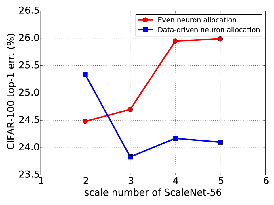
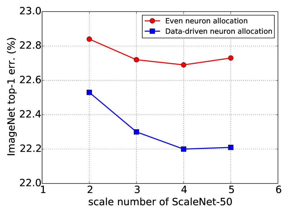
Figure 4: Comparisons between even neuron allocation and data-driven neuron allocation on CIFAR-100 and ImageNet.

The proposed ScaleNets can automatically learn the neuron proportion for each scale in each SA block. The neuron allocation depends on the training data distribution and network architectures.

Even allocation vs. data-driven allocation. Figure 4 compares even neuron allocation for scales in each SA block and data-driven neuron allocation. We conduct experiments on both CIFAR-100 and ImageNet with scale number $L$ from $2$ to $5$. Data-driven neuron allocation outperforms even allocation with impressive margins in all setting except that on CIFAR-100 with $L=2$. We also observe that data-driven allocation performs best on CIFAR-100 with $L=3$ and ImageNet with $L=4$. This is reasonable since ImageNet has bigger resolution and needs representation with wider scale range than CIFAR-100. We set $L$ to 3 on CIFAR-100 and $L$ to 4 on ImageNet in all our experiments except otherwise noted. Based on even allocation (gains from SA block), ScaleNet-50 achieves top-1 error rate of 22.76%. With data-driven allocation, the top-1 error rate can be further reduced to 22.20%.

Visualization of neuron allocation. Figure 5 shows learned neuron proportion in each SA block of ScaleNets. We observe that neuron proportions for scales are different from one SA block to another in one network. Specifically, scale 2 accounts for more and more proportion from bottom to top on both CIFAR-100 and ImageNet. Scale 4 mainly exists in the first two stages of ScaleNet-50 on ImageNet.

4.4 Object Detection on MS COCO

To further evaluate the generalization on other recognition tasks, we conduct object detection experiments on MS COCO [21] consisting of 80k training images and 40k validation images, which are further split into 35k miniusmini and 5k mini-validation set. Following the common setting [9], we combine the training images and miniusmini images and thus obtain 115k images for training, and the 5k mini-validation set for evaluation. We employ the Faster RCNN framework [25]. We test models by resizing the shorter edge of image to 800 (or 600) pixels, and restrict the max size of the longer edge to 1200 (or 1000).

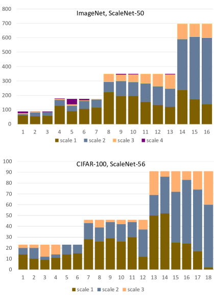
Figure 5: Neuron proportion for scales in each SA block of ScaleNets on CIFAR-100 and ImageNet.

Comparisons with baselines. Table 6 compares the detection results of ScaleNets and their baseline ResNets on MS COCO. With multi-scale aggregation, Faster RCNN achieves impressive gains with range from $3.2$ to $4.9$. Especially, ScaleNet-101 reaches an mmAP of 39.5.

	600/1000				800/1200
	mmAP	APs	APm	APl	mmAP	APs	APm	APl
ResNet-50	31.7	12.6	35.9	48.3	32.6	15.9	36.7	46
ScaleNet-50	36.2	17.1	40.7	53.8	37.2	19.4	41.3	52.6
ResNet-101	34.1	13.8	38.6	51	35.9	17.7	39.9	51.6
ScaleNet-101	37.3	16.6	42.4	55.1	39.5	21.3	44	55.2

Table 6: Comparisons of mAP on MS COCO. mmAP indicates the results of mAP@IoU=[0.50:0.95]. Results of ResNets and ScaleNets are obtained by keeping all settings the same except backbone for fair comparison.

ScaleNets are effective for object detection. Table 7 compares the effectiveness of backbones for object detection. It has been shown that ScaleNet-101 achieves the best detection performance with the minimal computational complexity amongst ResNets, ResNeXts [31], SE-ResNets [11], and Xception [5].

	ImageNet		COCO
	top-1 err.	FLOPs	mAP (600/1000)
ResNet-152	$21.58$	$11.5$	$34.3$
Xception	$21.11$	$9.0$	$27.7$
SE_ResNet-152	$21.07$	$11.5$	$37.1$
ResNeXt-101	$21.01$	$8.0$	$36.7$
ScaleNet-101	$20.97$	$\boldsymbol{7.5}$	$\boldsymbol{37.3}$

Table 7: Comparisons of effectiveness of backbone for object detection on MS COCO. All models are trained with the same strategy for fair comparison.

4.5 Analysis

The role of max pool. Downsampling can be implemented in several ways: (i) a $3\times 3$ conv with stride $s$; (ii) a dilated $3\times 3$ conv with stride $s$ [23]; (iii) a $s\times s$ avg pool with stride $s$; (iv) a $s\times s$ max pool with stride $s$. We evaluate all the above settings with ScaleNet-56 on CIFAR-100 by setting scale number $L$ to 2 and $s$ to 2 for simplicity. As shown in Table 8, (iv) performs best. It suggests that max pool is the key factor of performance boosting. It is reasonable since max pool preserves and enhances the maximum activation from previous layers so that the high response of small foreground regions would not be drowned by background features as information flows from bottom to top.

method	top1 err.
stride 2 of $3\times 3$ conv	26.19
stride 2 of $3\times 3$ conv, dilated 2	25.42
$2\times 2$ average pool	24.58
$2\times 2$ max pool	24.48

Table 8: Top-1 error rate on CIFAR-100 with different downsampling methods. All the methods are of same FLOPs and record the best result in 5 runs.

Wide range of receptive field. Figure 6 compares the receptive field range of each block. It has been shown that the proposed ScaleNets have much wider range of receptive field than others. Particularly, ScaleNet-50 reaches the resolution for classification and detection only in second and third block. On the one hand, ScaleNets potentially aggregate rich representations with large range of scales. On the other hand, they can extract global context information at very early stage (e.g., block 3) in one network. Together with data-driven neuron allocation, ScaleNets perform effectively and efficiently on various visual recognition tasks.

5 Conclusion

In this paper, we proposed a scale aggregation block with data-driven neuron allocation. The SA block can replace $3\times 3$ conv in ResNets to get ScaleNets. The data-driven neuron allocation can effectively allocate the neurons to suitable scale in each SA block. The proposed ScaleNets have wide range of receptive fields, and perform effectively and efficiently on image classification and object detection. We will test our ScaleNets on more computer vision tasks, such as segmentation [22], in the future.

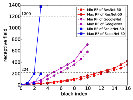
Figure 6: Comparisons of receptive field of multi-branch networks as a function of block index. The shortcut branch and residual branch in each residual block of ResNets have the minimal and maximal receptive field respectively. The $1\times 1$ conv branch, and 5×5 conv branch in each Inception block of GoogleNet have the minimal and maximal receptive field respectively.

6 Acknowledgement

This work was supported by Beijing Municipal Science and Technology Commission (Z181100008918004) in part. We thank Zhanglin Peng, Youjiang Xu, Xinjiang Wang, and Huabin Zheng from SenseTime for the helpful suggestions and supports.

Appendix A. Training Curves on ImageNet

Figure 7 compares the top-1 error rate of ResNets and ScaleNets on both ImageNet training and validation dataset. It has been shown that ScaleNets achieve much lower error rates than their counterpart ResNets during all training phase.

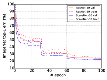
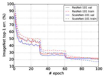
Figure 7: Comparison of the training curves. The left compares scale ScaleNet-50 and ResNet-50 on ImageNet training set and validation set, while the right compares ScaleNet-101 and ResNet-101.

Appendix B. Comparison with Pruning

To demonstrate the advantages comparing with pruning, we list the stage-of-art pruning methods and ScaleNet-50-light in Table 9.

	top-1 acc.$\uparrow$	FLOPs (109)$\downarrow$
CP-ResNet-50 [1, 10]	-3.68	1.5
SSS-ResNet-50 [14]	-1.94	1.3
NISP-ResNet-50 [33]	-0.21	1.1
LCP-ResNet-50 [7]	+0.09	1.0
ScaleNet-50-light	+0.98	1.2

Table 9: Comparison with state-of-the-art methods on ImageNet. ResNet-50 and ScaleNet-50-light are trained in same settings, and others are reported in their papers.

	top-1 err.	FLOPs($19^{9}$)	GPU time(ms)
ResNet-50	24.02	4.1	95
SE-ResNet-50	23.29	4.1	98
ResNeXt-50	22.2	4.2	147
ScaleNet-50	22.2	3.8	93

Table 10: Comparison of GPU time (averaging on 1000 runs).

Appendix C. GPU time

In Table 10 all networks were tested using Tensorflow with GTX 1060 GPU and i7 CPU at batch size 16 and image size 224. It has been shown that ScaleNet-50 achieves the best accuracy on ImageNet while with the least GPU running time.

Appendix D. Allocated Neuron Numbers of ScaleNets

Table 11 lists the detailed allocated neuron numbers of $3\times 3$ conv in SA block on ImageNet and CIFAR-100.

block index	ScaleNets for CIFAR-100			ScaleNets for ImageNet
	38 layers	56 layers	101 layers	50 layers (light)	50 layers	101 layers	152 layers
1	6,2,14	14,6,3	10,6,7	30,8,10,16	62,9,5,12	61,11,7,7	39,27,10,14
2	15,6,1	10,10,3	5,5,13	30,9,9,16	55,27,5,1	56,23,4,3	45,32,8,5
3	16,5,1	9,3,11	8,4,11	30,27,7,0	59,26,0,3	59,24,3,0	46,36,8,0
4	16,6,0	11,3,9	12,8,3	59,55,13,1	125,41,6,3	123,41,1,6	55,26,35,63
5	30,12,1	14,9,0	11,6,6	59,43,8,18	90,39,9,37	126,38,1,6	89,44,19,27
6	24,15,4	15,8,0	9,9,5	59,57,12,0	106,56,4,9	127,41,3,0	93,62,14,10
7	26,16,1	28,15,3	9,11,3	59,59,9,1	116,56,3,0	127,41,3,0	110,43,12,14
8	27,13,3	26,13,7	13,8,2	117,65,71,3	223,71,55,0	220,86,35,0	109,54,13,3
9	47,17,22	29,15,2	12,9,2	107,16,33,100	196,104,44,5	186,64,55,36	119,59,0,1
10	30,38,18	26,16,4	15,8,0	111,49,62,34	195,98,52,4	156,25,53,107	106,70,3,0
11	26,52,8	30,14,2	16,7,0	106,61,61,28	155,128,66,0	191,44,52,54	114,65,0,0
12	23,51,12	12,25,9	30,14,2	99,71,59,27	134,129,86,0	181,53,83,24	224,102,31,1
13		50,19,22	23,14,9	76,50,67,63	120,127,98,4	221,82,34,4	163,49,68,78
14		52,34,5	28,14,4	141,182,189,0	237,354,106,0	177,62,90,12	115,65,73,105
15		25,47,19	23,15,8	83,9,185,235	172,435,90,0	130,75,102,34	143,107,71,37
16		24,59,8	26,17,3	77,16,184,235	138,462,97,0	206,71,55,9	144,97,92,25
17		17,57,17	26,16,4			203,83,53,2	195,87,60,16
18		2,58,31	21,22,3			207,73,54,7	198,77,62,21
19			24,22,0			245,84,12,0	168,139,43,8
20			19,18,9			221,103,17,0	80,80,71,127
21			28,18,0			221,100,20,0	138,88,93,39
22			22,20,4			158,99,84,0	107,93,65,93
23			53,15,24			220,106,15,0	230,103,25,0
24			30,43,19			173,92,73,3	182,132,40,4
25			61,27,4			135,122,84,0	179,114,53,12
26			52,35,5			109,71,132,29	220,76,53,9
27			42,45,5			147,94,93,7	227,118,13,0
28			43,45,4			191,108,42,0	196,110,51,1
29			43,47,2			127,95,113,6	232,118,8,0
30			6,50,36			203,117,21,0	224,114,20,0
31			4,51,37			282,377,23,0	214,100,43,1
32			22,57,13			279,388,15,0	139,114,97,8
33			9,60,23			84,442,155,1	198,113,47,0
34							151,87,115,5
35							171,103,83,1
36							172,104,72,10
37							205,88,65,0
38							170,122,64,2
39							170,98,81,9
40							223,101,32,2
41							192,114,52,0
42							112,99,134,13
43							109,116,130,3
44							110,90,118,40
45							194,115,49,0
46							178,135,45,0
47							209,135,14,0
48							341,368,6,0
49							363,348,4,0
50							311,398,6,0

Table 11: Learned neuron numbers in each SA block in ScaleNets on CIFAR-100 and ImageNet. These numbers indicates the output channel numbers for scale 1, 2, 3, and 4 (e.g. $\text{3\texttimes 3 conv}_{[C_{1},C_{2},C_{3},C_{4}]}$ in Table 1). Note that ScaleNets on CIFAR-100 have only three scales.

References

- [1] https://github.com/yihui-he/channel-pruning.
- [2] J. M. Alvarez and M. Salzmann. Learning the number of neurons in neep networks. In NIPS, pages 2270–2278. 2016.
- [3] S. Bell, C. Lawrence Zitnick, K. Bala, and R. Girshick. Inside-outside net: Detecting objects in context with skip pooling and recurrent neural networks. In CVPR, pages 2874–2883, 2016.
- [4] X. Cao, Z. Wang, Y. Zhao, and F. Su. Scale aggregation network for accurate and efficient crowd counting. In ECCV, pages 734–750, 2018.
- [5] J. Carreira, H. Madeira, and J. G. Silva. Xception: A technique for the experimental evaluation of dependability in modern computers. IEEE Transactions on Software Engineering, 24(2):125–136, 1998.
- [6] X. Chen. Adaptive multi-scale information flow for object detection. In BMVC.
- [7] T.-W. Chin, C. Zhang, and D. Marculescu. Layer-compensated pruning for resource-constrained convolutional neural networks. arXiv preprint, 2018.
- [8] A. Gordon, E. Eban, O. Nachum, B. Chen, H. Wu, T.-J. Yang, and E. Choi. Morphnet: Fast & simple resource-constrained structure learning of deep networks. In CVPR, 2018.
- [9] K. He, X. Zhang, S. Ren, and J. Sun. Deep residual learning for image recognition. CVPR, pages 770–778, 2016.
- [10] Y. He, X. Zhang, and J. Sun. Channel pruning for accelerating very deep neural networks. In ICCV, 2017.
- [11] J. Hu, L. Shen, and G. Sun. Squeeze-and-excitation networks. In CVPR, 2018.
- [12] G. Huang, D. Chen, T. Li, F. Wu, L. van der Maaten, and K. Weinberger. Multi-scale dense networks for resource efficient image classification. In ICLR, 2018.
- [13] G. Huang, Z. Liu, L. Van Der Maaten, and K. Q. Weinberger. Densely connected convolutional networks. In CVPR, volume 1, page 3, 2017.
- [14] Z. Huang and N. Wang. Data-driven sparse structure selection for deep neural networks. In ECCV, pages 304–320, 2018.
- [15] S. Ioffe and C. Szegedy. Batch normalization: Accelerating deep network training by reducing internal covariate shift. In ICML, pages 448–456, 2015.
- [16] T. Kong, A. Yao, Y. Chen, and F. Sun. Hypernet: Towards accurate region proposal generation and joint object detection. In CVPR, pages 845–853, 2016.
- [17] A. Krizhevsky and G. Hinton. Learning multiple layers of features from tiny images. Technical report, 2009.
- [18] A. Krizhevsky, I. Sutskever, and G. E. Hinton. Imagenet classification with deep convolutional neural networks. In NIPS, pages 1097–1105, 2012.
- [19] V. Lebedev and V. Lempitsky. Fast convnets using group-wise brain damage. In CVPR, pages 2554–2564, 2016.
- [20] T.-y. Lin, P. Doll, R. Girshick, K. He, B. Hariharan, S. Belongie, F. Ai, and C. Tech. Fpn feature pyramid networks for object detection. CVPR, 2017.
- [21] T.-Y. Lin, M. Maire, S. Belongie, J. Hays, P. Perona, D. Ramanan, P. Dollár, and C. L. Zitnick. Microsoft coco: Common objects in context. In ECCV, pages 740–755, 2014.
- [22] J. Long, E. Shelhamer, and T. Darrell. Fully convolutional networks for semantic segmentation. In CVPR, pages 3431–3440, 2015.
- [23] D. I. C. Onvolutions. Multi-scale context aggregation by dilated convolutions. In ICLR, 2016.
- [24] A. Rabinovich and A. C. Berg. Parsenet looking wider to see better. pages 1–11, 2016.
- [25] S. Ren, K. He, R. Girshick, and J. Sun. Faster R-CNN: towards real-time object detection with region proposal networks. PAMI, 39(6):1137–1149, 2017.
- [26] S. Saxena and J. Verbeek. Convolutional neural fabrics. In D. D. Lee, M. Sugiyama, U. V. Luxburg, I. Guyon, and R. Garnett, editors, NIPS, pages 4053–4061. Curran Associates, Inc., 2016.
- [27] R. K. Srivastava, K. Greff, and J. Schmidhuber. Highway networks. arXiv preprint, 2015.
- [28] C. Szegedy, W. Liu, Y. Jia, P. Sermanet, S. Reed, D. Anguelov, D. Erhan, V. Vanhoucke, and A. Rabinovich. Going deeper with convolutions. In CVPR, pages 1–9, 2015.
- [29] T. Veniat and L. Denoyer. Learning time/emory-efficient deep architectures with budgeted super networks. arXiv preprint, 2017.
- [30] P. M. Williams. Bayesian regularization and pruning using a laplace prior. Neural computation, 7(1):117–143, 1995.
- [31] S. Xie, R. Girshick, P. Dollár, Z. Tu, and K. He. Aggregated residual transformations for deep neural networks. In CVPR, pages 5987–5995. IEEE, 2017.
- [32] F. Yu, D. Wang, E. Shelhamer, and T. Darrell. Deep layer aggregation. In CVPR, 2018.
- [33] R. Yu, A. Li, C.-F. Chen, J.-H. Lai, V. I. Morariu, X. Han, M. Gao, C.-Y. Lin, and L. S. Davis. Nisp: Pruning networks using neuron importance score propagation. In CVPR, 2018.
- [34] H. Zhao, J. Shi, X. Qi, X. Wang, and J. Jia. Pyramid scene parsing network. In CVPR, pages 2881–2890, 2017.
- [35] B. Zoph and Q. V. Le. Neural architecture search with reinforcement learning. arXiv preprint, 2016.