A Differential Approach for Gaze Estimation

Abstract

Most non-invasive gaze estimation methods regress gaze directions directly from a single face or eye image. However, due to important variabilities in eye shapes and inner eye structures amongst individuals, universal models obtain limited accuracies and their output usually exhibit high variance as well as subject dependent biases. Thus, increasing accuracy is usually done through calibration, allowing gaze predictions for a subject to be mapped to her actual gaze. In this paper, we introduce a novel approach, which works by directly training a differential convolutional neural network to predict gaze differences between two eye input images of the same subject. Then, given a set of subject specific calibration images, we can use the inferred differences to predict the gaze direction of a novel eye sample. The assumption is that by comparing eye images of the same user, annoyance factors (alignment, eyelid closing, illumination perturbations) which usually plague single image prediction methods can be much reduced, allowing better prediction altogether. Furthermore, the differential network itself can be adapted via finetuning to make predictions consistent with the available user reference pairs. Experiments on 3 public datasets validate our approach which constantly outperforms state-of-the-art methods even when using only one calibration sample or those relying on subject specific gaze adaptation.

1 Introduction

Gaze is an important cue of human behaviours. Gaze directions and gaze changing behaviours (such as gaze aversion, the intentional redirection away from the face of interlocutor [1]) are good indicators of the visual attention and are also related to internal thoughts or mental states of people. Besides, as a non-verbal behaviour, gaze is an important communication cue which has also been shown to be related to higher-level characteristics such as personality. It thus finds applications in many domains like Human-Robot-Interaction (HRI)[1, 2], Virtual Reality [3], social interaction analysis [4], or health care [5], or mobile phone scenarios [6, 7, 8].

Motivation. Non-invasive vision based gaze estimation has been addressed with two main paradigms: geometric models and appearance [9]. Since the former suffers from noise, image resolution, illumination, or head pose issues, appearance-based methods which predict gaze directly from the eye (or face) images have attracted more attentions in recent years [10, 11, 12, 13]. Among them, deep neural networks (DNN) have been shown to work well.

Nevertheless, even when using DNN regressors, their accuracy has been limited to around $5$ to $6$ degrees, with a high inter person variance [10, 11, 12, 13, 14, 15, 16]. This is due to many factors including dependencies on head poses, large eye shape variabilities, and only very subtle eye appearance changes when looking at targets separated by such small angle differences.

For instance, Fig. 1(a) shows the difficulty to define an absolute head pose like a frontal pose. This has a non negligible impact on the eye appearance. Another factor explaining the limited accuracy when building person independent models is that the visual axis is not aligned with the optical axis (related to the observed iris) [17], and that such alignment differences are subject specific (see Fig. 1(b)), with a standard deviation of 2 to 3 degrees amongst the population without eye problems. Said differently, in theory, images of two eyes with the same appearance but with different internal eyeball structure can correspond to different gaze directions, demonstrating that gaze can not be fully predicted from the visual appearance. Altogether, in practice, such variabilities introduce confusions for regression, as illustrated in Fig. 2 which shows that gaze related elements (like iris location or the eyelid closing) in eye images from different persons sharing the same gaze directions can look quite different, while more importantly, eye of different persons can be similar when they look at different directions (see (a-2) and (d-3)).

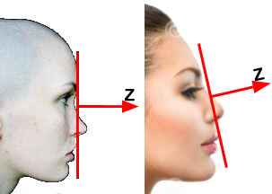
a) b)

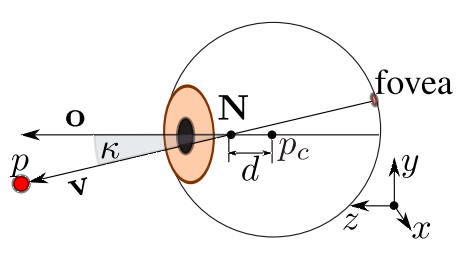
Figure 1: Examples of variability factors. (a) Head pose shape variabilities induce different frontal head pose definition and hence variabilities in eye images. (images from Pinterest.com). (b) Variabilities across subjects of the difference between the visual axis (unobserved, defining gaze) and the optical axis (defined by iris center, observed) introduces gaze prediction uncertainties (image from [18]).

A straightforward solution to this problem is to learn person-specific models [19, 10, 20] or fine-tune a pre-trained model [21]. Note that even regular high-end Infra-Red (IR) devices (eg from Tobii) require users to stare at several fixed positions before using them. However, training person-specific appearance models may require large amounts of personal data, especially for DNN methods and even when conducting simple network fine tuning adaptation. Other methods rely on fewer reference samples to train a linear regression model [22] or an SVR [6]. Still these methods are usually not robust to environment changes and their accuracy is heavily affected by the number of reference samples. A too small amount can even result in worse performance than without calibration. This is unfortunate, as there are plenty of real scenarios in which we can collect a few annotated samples.

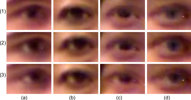
Figure 2: Appearance comparison. Columns (a) to (d) show right eye images from different persons from the EYEDIAP dataset [23]. Row (1) to (3) correspond to gaze directions with the same pitch (5 degrees) and a yaw of 5, 10, 15 degrees respectively.

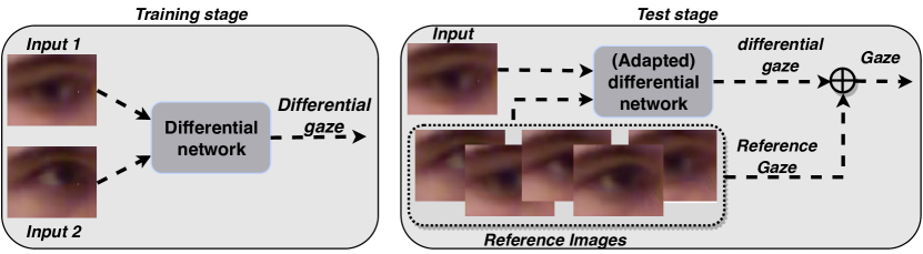
Figure 3: Approach overview. During training, random pairs of samples from the same eye are used to train a differential network. At test time, given a set of reference samples, gaze differences are computed and used to infer the gaze of the input image. To gain higher accuracy, the differential network can be adapted via fine-tuning using the pairs of reference samples.

Contributions. This paper is an extension of our paper [24]. we aim to solve the person-specific bias using a few annotated reference samples from the specific person. To this end, two strategies have been considered and analyzed. The first one is a baseline and consists of learning the linear relationship between the gaze predictions from a pre-trained NN applied to few training samples and their groundtruth gaze. Interestingly, although simple, it is shown to achieve better results than the state-of-the art SVR method of [6].

The second method corresponds to our main contribution, and is as follows. Although the previous methods can reduce the subject specific bias between the subject (test) data and the overall training dataset, it does this by only working with the gaze prediction or feature outputs, and does not account for the high gaze prediction variance within each subject’s data. To address this issue, we propose a differential gaze estimation approach, by training a differential NN to predict the gaze difference between two eye images instead of predicting the gaze directly. We hypothesize such a differential approach is less problematic than predicting gaze because the person dependent error (such as shape, alignment errors) will be alleviated. This is illustrated in Fig. 2, which shows that given an eye of a person, it is easier to judge whether it is looking more to the left or the right than a second eye image if the latter come from the same person than if it comes from another person (even with a similar eye shape). In Fig. 2, it is easier to see that the eye images at the bottom look more to the right than the eye images at top which are in the same column than compared to images in the other columns.

Our framework is illustrated in Fig. 3. At training time, a unified and person independent differential gaze prediction model is built which can be used at test time for person specific gaze inference relying on only a few calibration samples.

Thirdly, as there are many architectures that can be designed for differential gaze (early fusion by concatenating the two images, or fusion of feature maps of the two images at different levels), we investigate and compare different architectures and show that mid-level fusion is better than early fusion or late fusion. Usually they have different impacts on gaze estimation.

Paper organization. We discuss related works in Section 2. In Section 3, we introduce a state-of-the-art NN for gaze prediction, illustrate the subject specific bias problem, and present a baseline linear adaptation method to build subject specific gaze prediction models. In Section 4, we introduce our approach and the proposed modified siamese NN for differential gaze prediction. Experiments are presented in Section 5, while Section 6 concludes the work.

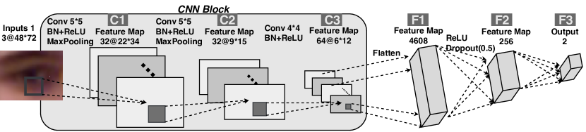
Figure 4: Baseline CNN structure for gaze estimation.

2 Related works

Our work relates to appearance-based modeling, person dependent calibration methods, and to some extend, to siamese network approaches for achieving other tasks.

2.1 Appearance-based gaze estimation

As said earlier, geometric approaches rely on eye feature extraction (like glints when working with infrared systems, eye corners or iris center localization) to learn a geometric model of the eye and then infer gaze direction using these features [25, 26, 27, 28, 29, 30]. However, they usually require high resolution eye images for robust and accurate feature extraction, are prone to noise or illumination perturbations, and do not handle well head pose variabilities.

Hence, many recent methods rely on an appearance based paradigm  [10, 11, 12, 13], exhibiting more robustness with low to mid-resolution images and obtaining good generalization performance. There, Neural networks (NN) methods have been shown to work well due to their ability to leverage large amount of data to train a regression network capturing the essential features of the eye images under various conditions like illumination and self-shadow, glasses, impact of head pose. For instance, [10] relied on a simple LeNet shallow network applied to eye images and first demonstrated that NNs outperform most other methods. Very recently, a deeper pretrained network (VGG-16 [31]) was fine-tuned for gaze estimation and further improved the accuracy [32]. In other directions, Krafka et. al [6] proposed to combine eye and face together using a multi-channel network, Zhang et. al [15] trained a weighted network to predict gaze from a full face image. Shrivastava et. al [14] learned a model from simulated eye images using a generative adversarial network.

2.2 Person dependent calibration

Person dependent calibration is critical to obtain a more robust and accurate model for gaze estimation (this is also the case for infrared head mounted device [33, 34]). To solve this problem, Lu et.al [22] proposed an adaptive linear regression method relying on few training samples, but the eye representation (multi-grid normalized mean eye image) is not robust to environmental changes. Starting from a trained NN, Krafka et.al. [6] relied on feature maps from the last layer of a pretrained NN to train a Support-Vector-Regression (SVR) person specific gaze prediction model from 13 reference samples. However, SVR regression from a high dimensional feature vector input is not robust to noise. Different from [6], Masko tried to fine-tune the last layer of a pre-trained model for each subject, but this requires large amounts of data. In another direction, Zhang et.al. [35] proposed to train person-specific gaze estimators from user interactions with multiple devices, such as mobile phone, tablet, laptop, or smart TVs, but this does not correspond to the majority of use cases.

However, none of the above works have proposed to calibrate gaze by estimating gaze difference from reference images, which as we show in this paper is a much more robust approach requiring less reference images.

2.3 Siamese network

They have first been proposed in [36] for signature verification, and with the deep learning revival, for tasks like feature extraction [37, 38], image matching and retrieval [39], one-shot recognition [40], person re-identification [41]. They consist of two parallel networks with shared weights, a pair of images as input (one per network), and the distance between their outputs is the siamese network output. Often, for classification, the goal is to learn an embedding space, where samples from the same class are close and samples from different classes are far. In regression, the loss function compares the output distance with the groundtruth one. Venturelli et.al. [42] use such an approach for head pose estimation. However, they use a multi-task approach in which both absolute poses and head pose differences are used as loss function. At test time, the pose is still directly predicted from a single image. Hence, while several layers of our differential networks are used to predict the gaze difference, in their case the pose differences was only computed from the network pose prediction output.

The few-shot learning approach of [43] is closer to our work. Authors rely on a relation network trained to compare images. As for us, its architecture consists of an embedding module that extracts featuremaps of images, and a relation module using the concatenated featuremaps as input to calculate a relation score. Their method however addresses a quite different task (image classification vs gaze regression), with a different loss function and they do not further adapt the network using the reference samples.

3 Baseline CNN approach and linear adaptation

(a) (b)

Figure 5: Scatter plot of the network regression (X-axis) and labelled groundtruth (Y-axis) of the yaw (left plot) and pitch (right plot) angles for an individual eye taken in the (a) EYEDIAP dataset; and (b) MPIIGaze dataset.

We first introduce a standard convolution neural network (CNN) for person independent gaze estimation. We then show the resulting bias existing for unknown individuals, and present a baseline linear adaptation method to solve it.

3.1 Gaze estimation with CNN

Network structure. Fig. 4 presents the standard NN structure for gaze estimation. It consists of three convolutional layers and two fully connected layers. More precisely, the input eye image $I\in R^{M\times N\times C}$, where $(M,N,C)=(48,72,3)$ denote the dimensions and number of channels of the image, is first whitened. The convolutional layers are then applied and the resulting feature maps are flattened to be fed into the fully-connected layers. The predicted gaze direction $\mathbf{g}^{p}(I)\in R^{2\times 1}$ is regressed at the last layer. The details of the network parameters can be found in the figure.

Loss function. Denoting the gaze groundtruth of an eye image $I$ by $\mathbf{g}^{gt}(I)$, we used the following $\mathrm{L}1$ loss function:

$$\mathcal{L}=\frac{1}{|{\cal D}|}\sum_{I\in{\cal D}}\|\mathbf{g}^{p}(I)-\mathbf{g}^{gt}(I)\|_{1},$$ (1)

where ${\cal D}$ denotes the training dataset and $|\cdot|$ denotes the cardinality operator.

Network training. For eye images in the dataset, we first resize them into a fixed resolution $s=48\times 72$. Concretely, we up-sample the images using bilinear interpolation if their sizes are smaller than $s$ (MPIIGaze dataset). Otherwise, we randomly crop patches with size $s$ around eyes (EYEDIAP dataset). The input has either three channels for color images as shown in Fig. 4, or one channel for gray scale images.

The network is optimized with Adam method, with a learning rate initially set to $0.001$ and then divided by $2$ after each epoch. In our experiment, $10$ epochs are applied and proved to be sufficient. The mini batch size is $128$.

3.2 Bias analysis and baseline linear adaptation method

Because each individual eye has specific characteristics (including internal non-visible dimensions or structures), in practice, we often observe a data bias between the network regression $\mathbf{g}^{p}(I)$ and the labeled groundtruth $\mathbf{g}^{gt}(I)$ of the eye images $I\in{\cal D}_{Test}$ belonging to a single person. This is illustrated in Fig. 5, which provides a scatter plot of the $(\mathbf{g}^{p}(I),\mathbf{g}^{gt}(I))$ angle pairs in typical cases, which can be compared with the identity mapping (black lines).

As can be observed, there is usually a linear relationship between $\mathbf{g}^{gt}(I)$ and $\mathbf{g}^{p}(I)$, which is illustrated by the red lines in the plots. Thus, when a set ${\cal D}_{c}$ of sample calibration points of a user (usually 9 to 25 points) is available, it is possible to learn this relation and obtain an adapted gaze model $\mathbf{g}^{ad}$ by fitting a linear model

$$\mathbf{g}^{ad}(I)=A\,\mathbf{g}^{p}(I)+B$$ (2)

where $A\in R^{2\times 2}$ and $B\in R^{1\times 2}$ are the linear parameters of the model which can be estimated through least mean square error (LMSE) optimization using the calibration data.

4 Proposed differential approach

4.1 Approach overview.

The linear adaptation above allows to correct biases from the gaze output, but this does not really account for the specificity of a user’s eye, nor was the network trained to take into account the presence of biases. The method we propose aims at solving these issues. It is illustrated in Fig. 3. Its main part is a differential network designed and trained to predict the differences in gaze direction between two images of the same eye. At test time, the gaze differences between the input eye image and a calibration set of reference images are computed first. Then the gaze of the eye image is estimated by adding these gaze differences to the reference gazes. The calibration set could further be used to adapt the network by fine-tuning so that is makes better differential predictions between reference sample pairs. The details of the different components are introduced in the following paragraphs.

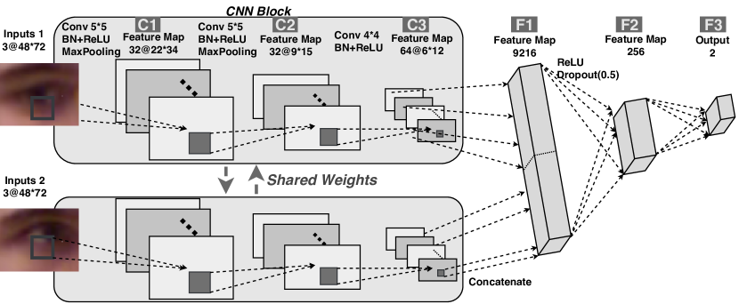
Figure 6: The designed differential network.

4.2 Differential network architecture.

The network we use is illustrated in Fig. 6. Each branch in the parallel structure is composed of three convolutional neural layers, all of them followed by batch normalization and ReLU units. Max pooling is applied after the first and second layers for reducing the image dimensions. After the third layer, the feature maps of the two input images are flatted and concatenated into a new tensor. Then two fully-connected layers are applied on the tensor to predict the gaze difference between the two input images. Thus, where traditional siamese approaches would predict the gaze for each image, and compute the differences from these predictions, our approach uses neural network layers to predict this difference from an intermediate eye feature representation.

The architecture we propose has several advantages. First, it is a good trade-off between prediction capacity and running-time. Secondly, while we could directly provide the two images as input to the network, this could increase the computational cost and not necessarily provide better prediction. We demonstrate this in the experimental section.

4.3 Loss function, network training and adaptation

The differential network is trained using a set of random image pairs $(I,J)$ coming from the same eye in the training data. Denoting by $\mathbf{d}^{p}(I,J)$ the gaze difference predicted by the network, we can define the loss function as:

$$\mathcal{L}_{diff}=\sum_{I,\,J\in{\cal D}^{k}}\|\mathbf{d}^{p}(I,J)-\left(\mathbf{g}^{gt}(I)-\mathbf{g}^{gt}(J)\right)\|_{1},$$ (3)

where ${\cal D}^{k}$ is the subset of ${\cal D}$ that only contains images of the same eye of person $k$.

Network training. Optimization is done with the Adam method and an initial learning rate of $0.001$ which is divided by $2$ after each epoch. In experiments, 20 epochs are applied. The mini batch size is $128$. To reduce the number of possible image pairs, we have constructed the dataset of pairs by using each image $I\in{\cal D}^{k}$ as first image and randomly selecting the second image $J$ in ${\cal D}^{k}$.

Network adaptation. At test time, since we are given a small calibration set ${\cal D}_{c}$ of reference images, we can fine-tune our network by selecting pair of samples $(I,\,J)\in{\cal D}_{c}$ and apply the same loss function  (3). In experiments, all possible pairs from ${\cal D}_{c}$ were used, and the same fine-tuning of 10 epochs with a fixed learning rate of 2e-4 was applied in all cases.

4.4 Gaze inference at test time.

Given the calibration dataset ${\cal D}_{c}$ of the user’s eye, we can first adapt the differential network (this is optional) as seen above. Then, we use the network to predict the gaze difference $\mathbf{d}^{p}$ ($I$, $F$) between the test image $I$ and the reference images $F$, and combine these gaze difference with the gaze groundtruth $\mathbf{g}^{gt}$ ($F$) to infer the gaze direction of the test image as $\mathbf{g}^{gt}$ ($F$)+ $\mathbf{d}^{p}$ ($I$, $F$). More formally:

$$\mathbf{g}^{sm}(I)=\frac{\sum_{F\in{\cal D}_{c}}w\left(\mathbf{d}^{p}(I,F)\right)\cdot\left(\mathbf{g}^{gt}(F)+\mathbf{d}^{p}(I,F)\right)}{\sum_{F\in{\cal D}_{c}}w\left(\mathbf{d}^{p}(I,F)\right)},$$ (4)

where $w(\cdot)$ is weighting the importance of each prediction.

Intuitively, if the reference eye image is more similar to the test eye image, we should be more confident about the gaze difference. Thus the weight has been defined as a function of $\mathbf{d}^{p}(I,F)$, which is a good indication of such similarity. In practice, we simply use a zero-mean Gaussian $\mathcal{N}(0,\sigma)$ as weight function. If $\sigma$ is too small, reference samples with large gaze difference will have no contribution. While if $\sigma$ is too large, reference samples will almost all have equal weights. In experiments, $\sigma=0.1$ radian (5.7 degrees) has been used on all datasets, although better values could be searched for per dataset using validation datasets within the training data.

5 Experimental results and analysis

In this section we thoroughly evaluate our algorithms and compare them with the-state-of-the-art methods on public datasets. In a second step, we discuss the impact of several important factors: choice and number of reference images, weighting scheme, architecture design, and model complexity.

5.1 Datasets

Since our method is designed for dealing with eye image alone, without extra information from the face, we considered the three following public eye-gaze datasets for validation.

EYEDIAP. It contains $94$ videos from 16 subjects [23]. Videos belong to three categories: continuous screen (CS) target, discrete screen (DS) target or floating target (FT). The CS videos were used in our experiments, which comprises static pose (SP) recordings (subjects approximately maintain the same pose while looking at targets), and dynamic poses (MP, subjects perform additional important head movements while looking). From this data, we cropped around $80K$ images of the left and right eyes and frontalized them according to [13]. The labeled world gaze groundtruth was converted accordingly in the Headpose Coordinate System (HCS).

MPIIGaze. This dataset [10] contains $1500$ left and right eye images of 15 subjects, which were recorded under various conditions in head pose or illuminations and contains people with glasses. The provided images are gray scale and approximately of size $36\times 60$ pixels, and are already frontalized relying on the head pose yaw and pitch. The provide gaze is labeled in Headpose Coordinate System (HCS). Note that although in [10] the head pose was used as input for gaze prediction, this did not improve our results in experiments so it was not used for the experiments reported below.

UT-Multiview. This dataset [19] comprises $23040$ (1280 real and 21760 synthesized) left and right eye samples for each of the 50 subjects (15 female and 35 male). It was collected under laboratory condition, with various head poses. Eye images are gray scale and of size $36\times 60$ pixels. They are not frontalized but accurate headpose and gaze in HCS are provided. Thus, in experiments, we concatenated the head pose in the network as described in [10]. More precisely, we concatenated the head pose $\mathbf{h}(I)\in R^{1\times 2}$ of the input $I$ image with the last fully-connected layers for the baseline CNN (Fig. 4), and did the same for the differential network, i.e. we concatenated the two head pose $\mathbf{h}(I)$ and $\mathbf{h}(J)$ of the input pair $(I,J)$ with the last fully-connected layer in Fig. 6.

5.2 Experimental protocol

Cross-Validation. For the EYEDIAP and MPIIGaze datasets, we applied a leave-one-subject-out protocol, while due to its size, we used a 3-fold cross-validation protocol for the UT-Multiview dataset. Note that for this dataset, we train with real and synthesis data, but only test on real data. Note that the protocols for MPIIGaze and UT-Multiview are the ones from the original paper and followed by other researchers.

Performance measure. Although nothing in the method prevents from using a single model for the left and right eyes through eye image mirroring, in experiments we trained and tested models for the left and right eyes separately. We noticed that there were some asymmetrical factors on the EYEDIAP dataset (see baseline results in Tab. I for instance) probably caused by differences in the preprocessing (e.g. the face mesh may fit closer or further away on different parts of the face depending on the viewpoint, which can affect the eye image normalization). Following the above protocols, the error was defined as the average of the average gaze angular error computed for each fold, according to [10].

Selection of reference samples. For the linear adaptation and the differential NN methods, unless stated otherwise, we randomly selected $9$ points as reference samples in the test set ${\cal D}_{Test}$ for $200$ times, and reported the average error computed for each random selection as defined above.

Tested models. Several methods were tested for comparison.

• Baseline: it corresponds to the generic model introduced in Section 2, and is our implementation of the neural network in [10], which achieves similar or better results than [10]. Note that [16] updates the result from [10] using a much deeper VGG-16 network. For real-time purpose, we use shallow networks, so we use our generic model as baseline for a fair comparison.

• SVR-Ad is our implementation of the SVR adaptation method of [6] built upon the Baseline model above. More precisely, following [6], the featuremap F2 (last layer before the output, see Fig. 4) is extracted as eye image features. A SVR model is trained using the reference image features and their gaze groundtruth.

• Lin-Ad corresponds to the Baseline model followed by linear adaptation (Section 2.2).

• Diff-NN: our differential network, with the default parameters introduced in the paper.

• Diff-NN-Ad: differential network adapted via parameter finetuning using reference samples (Section 4.3).

• Diff-NN^wo differential network Diff-NN without the Gaussian kernel averaging (corresponds to [24]).

• Diff-VGG differential network with a pre-trained VGG-16 backbone (same learning parameters as Diff-NN).

5.3 Experimental results

TABLE I: Average angular error (degree) on three public datasets. ‘L, R, Avg’ denote the left, right eyes and the average of them. Note that the Baseline method does not require calibration data.

	EYEDIAP			MPIIGaze			UT-multiview
	L	R	Avg	L	R	Avg	L	R	Avg
GazeNET [16]	-	-	-	-	-	5.5	-	-	4.4
Baseline [10]	5.37	6.63	6.00	5.97	6.25	6.11	6.08	5.83	5.95
SVR-Ad [6]	4.14	4.06	4.10	5.71	5.78	5.75	5.61	6.02	5.82
Lin-Ad	3.88	3.81	3.84	5.68	5.66	5.67	4.57	4.56	4.56
Diff-NN	3.23	3.23	3.23	4.69	4.62	4.64	4.17	4.08	4.13
Diff-NN-Ad	2.99	3.01	3.00	4.61	4.56	4.59	3.82	3.73	3.77
Diff-NNwo	3.37	3.35	3.36	4.73	4.61	4.67	4.41	4.24	4.33
Diff-VGG	3.19	3.06	3.12	3.88	3.73	3.80	3.88	3.68	3.78

The experimental results are presented in Table I.

Baseline model. First, let us note that under the same protocol, our Baseline model works slightly better than [10], which reported an error of $6.3{{}^{\circ}}$ on MPIIGaze, and of $5.9{{}^{\circ}}$ on UT-Multiview. This is probably due to our network architecture being slightly more complex, while still avoiding overfitting.

Linear and SVR Adaptation. Results demonstrate that, as expected, calibration helps and that the linear adaption method can greatly improve the baseline results, with an error decrease of (for the left and right eyes): $27.7\%$ and $43.3\%$ on EYEDIAP, $24.7\%$ and $21.8\%$ on UT-Multiview, and $4.9\%$ and $9.4\%$ on MPIIGaze. The difference in gain is most probably due to the recording protocols. While the EYEDIAP and UT-Multiview datasets were mainly recorded over the course of one session, the MPIIGaze dataset was collected in the wild, over a much longer period of time, and with much more lighting variability (but less head pose variability). This can be observed in Fig. 5 showing typical scattering plots of the EYEDIAP and MPIIGaze datasets. The EYEDIAP plots follow a more straight and compact linear relationship than those on the MPIIGaze dataset, reflecting the higher variability within the last dataset. Seen differently, we can interpret the results as having a session-based adaptation in the EYEDIAP and UT-Multiview cases, whereas in MPIIGaze, the adaptation is more truly subject-based.

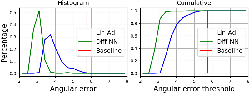
(a) (b)

Figure 7: Histogram and cumulative histogram of angular errors (in degree) due to the random selection of the calibration images, for (a) a given user and (b) all users of the MPIIGaze dataset, and for different methods: Diff-NN (green curve), Lin-Ad (blue curve), Baseline (red; in (b) the average result per user is used for the plot).

Results also show that the linear adaptation Lin-Ad method is working better than the SVR-Ad adaption approach [6], with an average gain of $6.3\%$, $1.4\%$ and $21.5\%$ on the EYEDIAP, MPIIGaze, and UT-Multiview datasets, respectively. The main reason might be that in SVR-Ad, the regression weights from the feature layer F2 are not exploited, in spite of their importance regarding gaze prediction. In addition, finding an appropriate kernel in the $256$ dimensional space of F2 might not be so easy, when using only $9$ samples.

Differential methods. Our approach Diff-NN performs much better than the other two adaptation methods which, on average over the 3 datasets, have an error $17.4\%$ (Lin-Ad) and $30.6\%$ (SVR-Ad) higher than ours. Interestingly, our method improves for all datasets and users on average compared to SVR-Ad, and similarly compared to Lin-Ad with the exception of 2 users (out of 50) in UT-Multiview. In particular, we can note that the gain is particularly important on the MPIIGaze dataset ($22.2\%$ compared to Lin-Ad), demonstrating that our strategy of directly predicting the gaze differences from pairs of images -hence allowing to implicitly match and compare these images- using our differential network is more powerful, and more robust against eye appearance variations across time, places, or illumination, than adaptation methods relying on gaze predictions only (Lin-Ad), or on compact eye image representations (SVR-Ad). To considering an even more realistic case, we randomly sampled the 9 reference samples from a single day and tested on the other days. The performance only dropped from 4.64 to $4.83^{\circ}$ error, showing the robustness of our method on this more ’subject-based’ adaptation dataset. On other more ’session-based’ datasets, the linear adaptation method is already doing well, so that the gain is lower (around $10\%$ on average). Note that removing the weighting scheme of Eq. 4 (Diff-NN^wo method) when combining per-reference gaze predictions [24] results in lower performance (around $0.2^{\circ}$), as further discussed in Sec. V.F.

Further gains can be obtained with our differential method. First, looking at the Diff-NN-Ad results, we see that even with few reference samples (9) a systematic finetuning of the differential network can further improve the results: results of Diff-NN are 7.5%, 1% and 9.5% higher than those of Diff-NN-Ad on EYEDIAP, MPIIGaze and UT-Multiview, respectively. Secondly and importantly, by simply using the deeper VGG-16 backbone to extract feature maps of the eye (instead of the C1-C3 CNN blocks, see Fig. 6), we can reduce the errors by 4, 9 and 18% on the EYEDIAP, UT-Multiview and MPIIGaze datasets, respectively. This is obtained at the cost of a higher memory footprint and computational complexity. It makes the model competitive with respect to the state of the art: for instance the adaptation method in [44] reported an error of $4.2^{\circ}$ on the MPIIGaze dataset, compared to $3.8^{\circ}$ in our case. The Diff-VGG results are similar to those of Diff-NN-Ad (except on MPIIGaze where it works much better). It is left as future work to see whether finetuning would further improve the results.

5.4 Cross-dataset experiments.

Such experiments are important and can be conducted to show a method generalization, as long as the preprocessing and task formulation are equivalent (e.g. addressing gaze estimation from face images, and using face datasets with the same gaze definition). Unfortunately, when working with existing cropped eye image datasets, there are factors which can limit the validity of cross-dataset experiments, as they clearly introduce systematic domain biases [45]. Such factors include using different gaze coordinate systems and data preprocessing methods, like geometric normalization relying on different head pose estimators or cropping paradigms.

Nevertheless, as our method relies on image pairs, one could hope that it would be robust to these domain shifts. To evaluate this, we trained methods using UT-Multiview and tested on MPIIGaze, which share a similar normalization goal (compared to EYEDIAP) but not the same pre-processing. Previous methods were reporting errors of $13.9^{\circ}$ [10] and $8.9^{\circ}$ [46] without any reference samples. This paper baseline method achieves an angular error of $17.8^{\circ}$. Errors of the Lin-Ad, SVR-Ad and Diff-NN methods are respectively 9.2, 9.7 and 9.8 using 9 reference samples, 8.4, 8.1 and 8.4 with 50 samples. While all adaptation methods improve the baseline results significantly, their performance remain far from the within dataset results (between 3.8 and 5.6). We believe this to be due in great part to preprocessing discrepancies, and significant head and eye poses distributions difference between the two datasets. Unfortunately, our approach does not provide additional robustness against such geometric domain shifts. Handling them require methods of its own which can leverage more (labeled or no) target domain data.

5.5 Impact of reference samples

In this section, we discuss the impact of the selection and number of reference samples on performance.

Calibration data variability. The performance of the adaptation methods are computed as the average over 200 random selections of $9$ calibration samples. Depending on the selection (samples might be noisy, or not distributed well on the gaze grid), results may differ. The left plot of Fig. 7(a) shows the histogram of the angular error of Lin-Ad and Diff-NN for the different trials of one subject and the right plot shows the cumulative histogram (percentage of trials whose performance is below a threshold). Fig. 7(b) does the same using the performance results of all users.

Fig. 7(a) shows an example where there is a relatively large bias for the given subject. In that case, whatever the selection of the calibration samples, the results of both Lin-Ad and Diff-NN are better than the baseline. However, importantly, our Diff-NN approach is much less sensitive to the choice of calibration points than Lin-Ad, as can be seen from the higher and concentrated peaks in the error distributions. In other examples, the baseline is better (the red bar is within or more towards the peaks of the variability histograms), but the behaviors and relative placements of the Lin-Ad and Diff-NN curves remain the same, as shown by looking at the statistics over all users in Fig. 7(b).

Reference sample selection. We can analyze the impact of the reference samples by measuring the error when using a single sample. To do so, for each user, we randomly select $200$ times one sample as reference, and then compute the errors for all test samples. The resulting statistics for all users are shown in Fig. 8, in which we plot the average angular error of the yaw prediction (respectively pitch and gaze) in function of the difference in yaw (respectively pitch and gaze) between the test and reference samples.

As expected, we observe that predictions are more accurate when test samples are closer to the reference sample (red curve) which justifies the use of the weighted sum in Eq. (4). Interestingly, we also notice that the error profile of the yaw is relatively flat, while that of the yaw is increasing. An explanation is that when comparing two eye images, aligning them laterally relies on relatively stable structures (eye corners), and the iris horizontal location (related to yaw) can be estimated reliably from strong vertical edges. However, visually, pitch estimation is much harder: the vertical alignment relies on eyelid contours, which are moving structures (correlated with the pitch, but only partially), and as the iris top and bottom parts are often hidden, the iris vertical position needs to be estimated from the shape of the iris vertical sides.

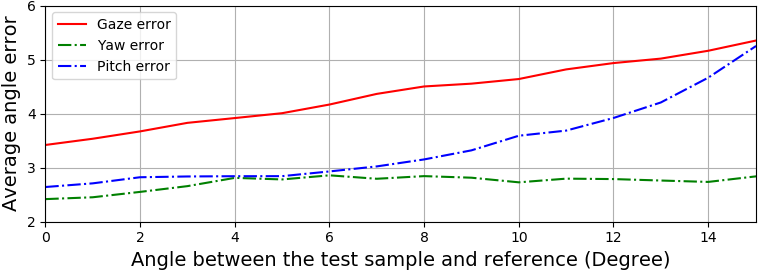
Figure 8: The average prediction error of the yaw in function of the absolute difference in yaw between the reference and test samples (green curve), and similarly for the pitch and gaze.

Discussion about the number of references. Fig. 9 presents adaptation results on the EYEDIAP dataset using different number of reference images. When given few reference samples, the SVR-Ad and Lin-Ad underperform the Baseline, which is mainly due to the noise illustrated in Fig. 5, which introduce a high variability (and error) in the fitting process, especially for Lin-Ad. As the number of reference samples increases, the error of Lin-Ad decreases significantly because more accurate linear parameters can be obtained for adaptation. The error of SVR-Ad decreases more slowly at the beginning, but catches up that of Lin-Ad when using more samples, due to the inherent ability of SVR-Ad at leveraging more reference samples.

The Diff-NN outperforms the other methods for small numbers even when using only one reference samples. This is not surprising because Diff-NN does not learn any model or parameter from the reference samples, but rather relies on richer information (the image context) to infer the difference rather than just the predicted gaze. However, with more samples, the SVR-Ad method works better, as the Support Vector principle might better handles larger amounts of data compared to our simpler weighting scheme, and the Diff-NN network prediction bias (and high variance) remains unchanged with more data. Our network adaptation strategy Diff-NN-Ad does not have this limitation, and indeed better leverage the availability of more reference samples. While for small amount of reference samples the improvement over Diff-NN is small (7.5%), with 25 samples, results of the Diff-NN and SVR-Ad methods are 23% and 29% higher than that of Diff-NN-Ad, and with 50 samples they are 35% and 27% higher.

Figure 9: Comparison of average angular error in degree (average of the left right eyes) for different methods in function of the number of reference images on EYEDIAP dataset. Note that the Baseline method does not require calibration data.

5.6 Reference weighting scheme

We analyse here the weighting scheme combining the predictions made from each reference image (see Eq. (4)) as well as the influence of the Gaussian kernel bandwidth $\sigma$. Intuitively, when $\sigma$ is too small, mainly the closest reference sample will contribute to the prediction. Conversely, when $\sigma$ is too large, reference samples will have similar contributions.

Results are shown in Fig. 10. When $\sigma$ varies from $5.7$ to $22.8$ degrees, the error stays low, changing in a narrow range of $0.1$. It indicates that the Diff-NN is very robust w.r.t the weights, as also observed on MPIIGaze and UT-Multiview.

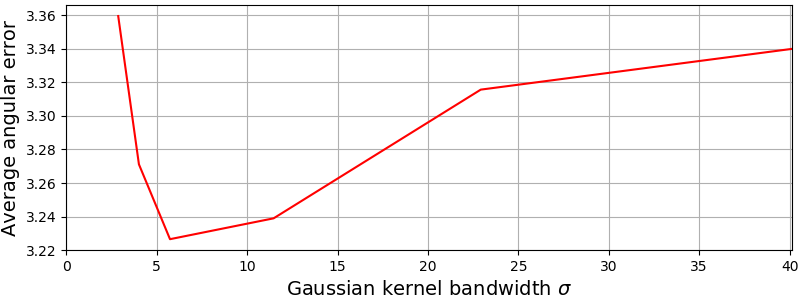
Figure 10: Average angular error (degree) on EYEDIAP dataset with different Gaussian kernel bandwidth $\sigma$ (in degree).

5.7 System design

Designing the network architecture can be motivated by several factors and principles. The main idea behind the differential network is that it can implicitly register and align images of the same eyes and from there better compute the (differential) elements (iris location, eye corners, eyelid closing) which really matters for gaze estimation than when abstracting these from a single image. We thus investigated different levels at which to fuse the information coming from the two eye images. Early fusion is achieved by using concatenated eye images as input to the network (See Fig. 4). It allows a direct comparison of the raw signals but suffers from increase complexities in (i) performing an implicit eye alignment if eyes are too far apart in the input images; (ii) abstracting important eye structures for gaze difference prediction, because the information coming from the two eyes is mixed in the layers. Also, the complexity increases, as all (input, reference) image pairs need to be fully processed. At the other end, late fusion can be conducted by concatenating the F2 feature maps of the two images. The F2 eye representation might contain high level eye representations tuned to the prediction of differential gaze, but there might be a loss of localization information.

Our proposed network lies in between. It relies on intermediate representations of each eye allowing in principle the implicit registration of the two eyes from the processed images while extracting high level information relevant for differential gaze regression. To verify the intuition behind the proposed scheme, we compared the following systems:

1. Sys-1 - early fusion: concatenate the two images;

2. Sys-2 - proposed : concatenate the F1 feature maps;

3. Sys-3 - late fusion: concatenate the F2 feature map;

4. Sys-4 - siamese: two parallel Baseline networks with shared weights trained to only predict gaze differences.

5. Sys-5 - multi-task with adaptation: it corresponds to Sys-4 but trained to predict both the absolute gaze and the difference (as in  [42] for head pose). The trained network is further adapted using the Lin-Ad scheme.

TABLE II: Average angular error (degree) on EYEDIAP dataset for different systems (see text).

Sys-1-early	Sys-2-proposed	Sys-3-late	Sys-4-siamese	Sys-5
3.40	3.23	3.47	3.40	3.76

Results are shown in Table II, and show that our architecture achieves the best results. Note that Sys-5 (approach of [42] followed by Lin-Ad) is worse than all other systems, demonstrating the advantage of predicting differential gaze over absolute gaze. The results of the Sys-1,3,4 are close but still outperformed by our system Sys-2, showing that intermediate fusion is better than early or late fusion. We believe this is due to the ability of the CNN network layers to do some filtering and alignment of the two images, while the fully-connected layers combine this information to infer gaze differences.

5.8 Algorithm complexity

The Diff-NN adaptation method does not have the same complexity as the others. Compared to the CNN Baseline, the linear adaptation only requires the computation of Eq.(2), which has negligible computational cost. Our Diff-NN approach, however, requires to predict the gaze differences between the test sample and $N_{c}$ reference images. Fortunately, its complexity is not $N_{c}$ times that of the Baseline thanks to our differential architecture (see Fig. 6). Indeed, we can pre-compute and save the feature maps at the last convolutional neural layer of all the reference images. Thus, the complexity reduces to the computation of the feature maps of the input image and of $N_{c}$ gaze differences from the feature maps, which can be done in parallel within a mini-batch.

Table III compares the running time (in ms) for the Baseline and the different Diff-NN options (and $N_{c}=9$). They have been obtained by computing the average run-time of processing $5000$ images. The CPU is an Intel(R) Core(TM) i7-5930K with 6 kernels and 3.50GHz per kernel. The GPU is an Nvidia Tesla K40. The program is written in Python and Pytorch. Note that as the Pytorch library will call multiple kernels for computation, the CPU-based run-time is also short. From this Table, we can see that our Diff-NN method and architecture has a computational complexity close to the Baseline.

TABLE III: Run-times (in ms) between the Baseline and our Diff-NN method, using mini-batch (Diff-NN $\!{}^{*}$) computation or not.

	CPU			GPU
	Baseline	Diff-NN	Diff-NN ∗	Baseline	Diff-NN	Diff-NN ∗
Run-time	2.5	7.6	3.5	1.4	4.0	1.5

6 Conclusion

This paper aims to improve appearance-based gaze estimation using subject specific models built from few calibration images. Our main contribution is to propose a differential NN for predicting gaze differences instead of gaze directions to alleviate the impact of annoyance factors like illumination, cropping variability, variabilities in eye shapes. Experimental results on three public and commonly used datasets prove the efficacy of the proposed methods. More precisely, while standard linear adaptation method can already boost the results on single session like situations, the differential NN method produces even more robust and stable results across different sessions of the same user, but costs some more run-time compared to a baseline CNN. Further fine-tuning of the network using the reference samples provide as well as very good mean to leverage larger amounts of calibration samples.

References

- [1] S. Andrist, X. Z. Tan, M. Gleicher, and B. Mutlu, “Conversational gaze aversion for humanlike robots,” in ACM/IEEE International Conference on Human-robot Interaction, 2014, pp. 25–32. [Online]. Available: http://doi.acm.org/10.1145/2559636.2559666
- [2] A. Moon, D. M. Troniak, B. Gleeson, M. K. Pan, M. Zheng, B. A. Blumer, K. MacLean, and E. A. Croft, “Meet me where i’m gazing: How shared attention gaze affects human-robot handover timing,” in ACM/IEEE Int. Conf. on Human-robot Interaction (HRI), 2014.
- [3] T. Pfeiffer, “Towards gaze interaction in immersive virtual reality: Evaluation of a monocular eye tracking set-up,” in Virtuelle und Erweiterte Realität-Fünfter Workshop der GI-Fachgruppe VR/AR, 2008.
- [4] R. Ishii, K. Otsuka, S. Kumano, and J. Yamato, “Prediction of who will be the next speaker and when using gaze behavior in multiparty meetings,” ACM Transactions on Interactive Intelligent Systems, vol. 6, no. 1, pp. 4:1–4:31, May 2016. [Online]. Available: http://doi.acm.org/10.1145/2757284
- [5] M. Vidal, J. Turner, A. Bulling, and H. Gellersen, “Wearable eye tracking for mental health monitoring,” Computer Communications, vol. 35, no. 11, pp. 1306–1311, 2012. [Online]. Available: http://dx.doi.org/10.1016/j.comcom.2011.11.002https://perceptual.mpi-inf.mpg.de/files/2013/03/vidal12_comcom.pdf
- [6] K. Krafka, A. Khosla, P. Kellnhofer, and H. Kannan, “Eye Tracking for Everyone,” IEEE Conference on Computer Vision and Pattern Recognition, pp. 2176–2184, 2016.
- [7] M. Tonsen, J. Steil, Y. Sugano, and A. Bulling, “Invisibleeye: Mobile eye tracking using multiple low-resolution cameras and learning-based gaze estimation,” ACM on Interactive, Mobile, Wearable and Ubiquitous Technologies, vol. 1, no. 3, 2017. [Online]. Available: https://perceptual.mpi-inf.mpg.de/files/2017/08/tonsen17_imwut.pdf
- [8] Q. Huang, A. Veeraraghavan, and A. Sabharwal, “Tabletgaze: unconstrained appearance-based gaze estimation in mobile tablets,” arXiv preprint arXiv:1508.01244, 2015.
- [9] D. W. Hansen and Q. Ji, “In the eye of the beholder: A survey of models for eyes and gaze,” IEEE T. on Pattern Analysis and Machine Intelligence, vol. 32, no. 3, pp. 478–500, 2010.
- [10] X. Zhang, Y. Sugano, M. Fritz, and A. Bulling, “Appearance-based gaze estimation in the wild,” in IEEE Conference on Computer Vision and Pattern Recognition. IEEE, jun 2015, pp. 4511–4520. [Online]. Available: http://ieeexplore.ieee.org/document/7299081/
- [11] Y. Sugano, Y. Matsushita, and Y. Sato, “Learning-by-synthesis for appearance-based 3d gaze estimation,” in IEEE Conf. on Comp. Vision and Pattern Recognition, 2014, pp. 1821–1828.
- [12] W. Zhu and H. Deng, “Monocular free-head 3d gaze tracking with deep learning and geometry constraints,” in The IEEE International Conference on Computer Vision, Oct 2017.
- [13] K. A. Funes Mora and J.-M. Odobez, “Gaze estimation in the 3d space using rgb-d sensors,” International Journal of Computer Vision, vol. 118, no. 2, pp. 194–216, 2016.
- [14] A. Shrivastava, T. Pfister, O. Tuzel, J. Susskind, W. Wang, and R. Webb, “Learning from simulated and unsupervised images through adversarial training,” in IEEE Conference on Computer Vision and Pattern Recognition, 2017, pp. 2107–2116.
- [15] C. Zhang, R. Yao, and J. Cai, “Efficient eye typing with 9-direction gaze estimation,” Multimedia Tools and Applications, pp. 1–18, 2017.
- [16] X. Zhang, Y. Sugano, M. Fritz, and A. Bulling, “It’s written all over your face: Full-face appearance-based gaze estimation,” in IEEE Int. Conf. on Computer Vision and Pattern Recognition Workshops, 2017.
- [17] E. D. Guestrin and M. Eizenman, “General theory of remote gaze estimation using the pupil center and corneal reflections,” IEEE Transactions on biomedical engineering, vol. 53, no. 6, pp. 1124–1133, 2006.
- [18] K. A. Funes Mora and J.-M. Odobez, “Geometric Generative Gaze Estimation (G 3 E) for Remote RGB-D Cameras,” pp. 1773–1780, jun 2014. [Online]. Available: http://ieeexplore.ieee.org/lpdocs/epic03/wrapper.htm?arnumber=6909625
- [19] Y. Sugano, Y. Matsushita, and Y. Sato, “Learning-by-synthesis for appearance-based 3d gaze estimation,” in IEEE Conf. on Comp. Vision and Pattern Recognition, 2014, pp. 1821–1828.
- [20] Z. Tősér, R. A. Rill, K. Faragó, L. A. Jeni, and A. Lőrincz, “Personalization of gaze direction estimation with deep learning,” in Joint German/Austrian Conference on Artificial Intelligence (Künstliche Intelligenz). Springer, 2016, pp. 200–207.
- [21] D. Masko, “Calibration in Eye Tracking Using Transfer Learning,” Ph.D. dissertation, KTH ROYAL INSTITUTE OF TECHNOLOGY, 2017.
- [22] F. Lu, Y. Sugano, T. Okabe, and Y. Sato, “Adaptive Linear Regression for Appearance-Based Gaze Estimation,” Pami, vol. 36, no. 10, pp. 2033–2046, 2014.
- [23] K. A. Funes Mora, F. Monay, and J.-M. Odobez, “Eyediap: A database for the development and evaluation of gaze estimation algorithms from rgb and rgb-d cameras,” in Proceedings of the Symposium on Eye Tracking Research and Applications. ACM, 2014, pp. 255–258.
- [24] G. Liu, Y. Yu, K. A. Funes-Mora, and J.-M. Odobez, “A differential approach for gaze estimation with calibration,” in The British Machine Vision Conference. The British Machine Vision Association, 2018.
- [25] E. Wood and A. Bulling, “Eyetab: Model-based gaze estimation on unmodified tablet computers,” ACM Symposium on Eye Tracking Research and Applications, pp. 3–6, 2014. [Online]. Available: http://dl.acm.org/citation.cfm?id=2578185
- [26] K. A. Mora Funes and J.-M. Odobez, “3D Gaze Tracking and Automatic Gaze Coding from RGB-D Cameras,” IEEE CVPR, Vision Meets Cognition Workshop, 2014.
- [27] R. Valenti, N. Sebe, and T. Gevers, “Combining head pose and eye location information for gaze estimation,” IEEE Transactions on Image Processing, vol. 21, no. 2, pp. 802–815, 2012.
- [28] L. Sun, M. Song, Z. Liu, and M.-T. Sun, “Real-time gaze estimation with online calibration,” IEEE MultiMedia, vol. 21, no. 4, 2014.
- [29] E. Wood, T. Baltrušaitis, L.-P. Morency, P. Robinson, and A. Bulling, “A 3d morphable eye region model for gaze estimation,” in European Conference on Computer Vision. Springer, 2016, pp. 297–313.
- [30] K. Wang and Q. Ji, “Real Time Eye Gaze Tracking with Kinect,” IEEE conference on Computer Vision, pp. 1003–1011, 2017.
- [31] K. Simonyan and A. Zisserman, “Very deep convolutional networks for large-scale image recognition,” arXiv preprint arXiv:1409.1556, 2014.
- [32] X. Zhang, Y. Sugano, M. Fritz, and A. Bulling, “MPIIGaze: Real-World Dataset and Deep Appearance-Based Gaze Estimation,” IEEE Trans. on Pat. Analysis and Machine Intelligence, pp. 1–14, 2017.
- [33] A. Lanata, G. Valenza, A. Greco, and E. P. Scilingo, “Robust head mounted wearable eye tracking system for dynamical calibration,” Journal of Eye Movement Research, vol. 8, no. 5, 2015.
- [34] Y. Sugano and A. Bulling, “Self-calibrating head-mounted eye trackers using egocentric visual saliency,” in ACM Symposium on User Interface Software & Technology, 2015, pp. 363–372.
- [35] X. Zhang, M. X. Huang, Y. Sugano, and A. Bulling, “Training person-specific gaze estimators from user interactions with multiple devices,” in Proceedings of the 2018 CHI Conference on Human Factors in Computing Systems. ACM, 2018, p. 624.
- [36] J. Bromley, I. Guyon, Y. LeCun, E. Säckinger, and R. Shah, “Signature verification using a” siamese” time delay neural network,” in Advances in Neural Information Processing Systems, 1994, pp. 737–744.
- [37] S. Zagoruyko and N. Komodakis, “Learning to compare image patches via convolutional neural networks,” in IEEE Conference on Computer Vision and Pattern Recognition. IEEE, 2015, pp. 4353–4361.
- [38] B. G. Kumar, G. Carneiro, I. Reid et al., “Learning local image descriptors with deep siamese and triplet convolutional networks by minimising global loss functions,” in IEEE Conference on Computer Vision and Pattern Recognition, 2016, pp. 5385–5394.
- [39] F. Wang, L. Kang, and Y. Li, “Sketch-based 3d shape retrieval using convolutional neural networks,” in IEEE Conference on Computer Vision and Pattern Recognition. IEEE, 2015, pp. 1875–1883.
- [40] G. Koch, R. Zemel, and R. Salakhutdinov, “Siamese neural networks for one-shot image recognition,” in ICML deep learning workshop, 2015.
- [41] R. R. Varior, M. Haloi, and G. Wang, “Gated siamese convolutional neural network architecture for human re-identification,” in European Conference on Computer Vision. Springer, 2016, pp. 791–808.
- [42] M. Venturelli, G. Borghi, R. Vezzani, and R. Cucchiara, “From depth data to head pose estimation: a siamese approach,” arXiv preprint arXiv:1703.03624, 2017.
- [43] F. Sung, Y. Yang, L. Zhang, T. Xiang, P. H. Torr, and T. M. Hospedales, “Learning to compare: Relation network for few-shot learning,” in Proceedings of the IEEE Conference on Computer Vision and Pattern Recognition, 2018, pp. 1199–1208.
- [44] Y. Yu, G. Liu, and J.-M. Odobez, “Improving few-shot user-specific gaze adaptation via gaze redirection synthesis,” in Proceedings of the IEEE Conference on Computer Vision and Pattern Recognition, June 2019.
- [45] ——, “Deep multitask gaze estimation with a constrained landmark-gaze model,” in The European Conf. on Computer Vision (ECCV) Workshops, Sept. 2018.
- [46] Y. Xiong, H. J. Kim, and V. Singh, “Mixed effects neural networks (menets) with applications to gaze estimation,” in Proceedings of the IEEE Conference on Computer Vision and Pattern Recognition, 2019, pp. 7743–7752.