Block preconditioning of stochastic Galerkin problems:
New two-sided guaranteed spectral bounds

Abstract

The paper focuses on numerical solution of parametrized diffusion equations with scalar parameter-dependent coefficient function by the stochastic (spectral) Galerkin method. We study preconditioning of the related discretized problems using preconditioners obtained by modifying the stochastic part of the partial differential equation. We present a simple but general approach for obtaining two-sided bounds to the spectrum of the resulting matrices, based on a particular splitting of the discretized operator. Using this tool and considering the stochastic approximation space formed by classical orthogonal polynomials, we obtain new spectral bounds depending solely on the properties of the coefficient function and the type of the approximation polynomials for several classes of block-diagonal preconditioners. These bounds are guaranteed and applicable to various distributions of parameters. Moreover, the conditions on the parameter-dependent coefficient function are only local, and therefore less restrictive than those usually assumed in the literature.

65F08, 65N22

1 Introduction

Growing interest in uncertainty quantification of numerical solutions of partial differential equations stimulates new modifications of standard numerical methods. A popular choice for partial differential equations with parametrized or uncertain data is the stochastic Galerkin method [4, 36]. Similarly to deterministic problems, approximate solutions, which depend on physical and stochastic variables (parameters), are searched for in finite-dimensional subspaces of the original Hilbert space. More precisely, the approximate solutions are orthogonal projections of the exact solution to the finite-dimensional subspaces with respect to the energy inner product defined by the operator of the equation; see, e.g., [5, 9, 10, 24]. The approximation subspaces are considered in the form of a tensor product of a physical variable space (finite-element functions) and a stochastic variable space (polynomials); see, e.g., [4, 14]. The form and qualities of the system matrix $\bm{A}$ of the discretized problem are determined by the structure of the uncertain data and the type of the finite-dimensional solution spaces. For special classes of parameters, it was shown, see, e.g., [24, 32], that certain block-diagonal matrices are spectrally equivalent to $\bm{A}$ independently of the degree of polynomials and the number of random parameters, and thus they can be used for preconditioning. Having a good preconditioning method or, in other words, a good and feasible approximation of $\bm{A}^{-1}$, we may also efficiently estimate a posteriori the energy norm of the error during iterative solution processes [1, 5, 6, 9, 17]. This estimate can be used in adaptive algorithms [5, 7, 8]. In practice, matrix $\bm{A}$ is never built explicitly, only matrix-vector products are evaluated ([25]).

In this paper, we focus on matrices arising in the discretized stochastic Galerkin method and present new guaranteed two-sided bounds to the spectra of the preconditioned matrices for several types of preconditioner. We consider only preconditioning with respect to the stochastic parts of problems, and thus we assume that a suitable preconditioning method or an efficient solver for the underlying deterministic problem is available; see, e.g., [12, 23, 33]. We formulate an idea of obtaining bounds to the spectra of the preconditioned matrix from the spectrum of small Gram matrices depending solely on the stochastic part of the approximation space. The motivation, however, comes from techniques and tools of the algebraic multilevel preconditioning introduced in [11, 2]. Similar idea was, in a simpler form, used already in [28, 29]. In the current paper, it is applied in a more general setting, and we believe that the derived technique may lead to an improvement of some other recently introduced estimates, such as [17, 23]. The derived technique is also applicable to systems in the form of multi-term matrix equation (see [25, eq. (1.8)]).

The paper is organized as follows. In Section 2, we briefly recall the stochastic Galerkin method and the structure of the matrices $\bm{A}$ of the resulting systems of linear equations for the tensor product polynomials and complete polynomials. Since the structure of $\bm{A}$ plays a crucial role in the analysis, theoretical considerations will be accompanied by illustrative examples throughout the paper. Section 3 formulates a general concept of proving spectral equivalence for a broad class of (not only) stochastic Galerkin preconditioners. In Section 4, we apply this idea to preconditioners which are represented by a special type of block-diagonal (or Schur complement) approximations of $\bm{A}$, and show how to obtain the spectral bounds of the preconditioned problems from the spectral bounds of small Gram matrices of the corresponding polynomial chaos. We also evaluate those bounds explicitly for the considered polynomial chaoses. Simple numerical examples demonstrating the obtained theoretical outcomes are presented at the end of the section.

Throughout the paper, we denote by $\kappa(\bm{M}^{-1}\bm{A})$, where $\bm{A}$ and $\bm{M}$ are symmetric positive definite, the spectral condition number of $\bm{M}^{-1}\bm{A}$, i.e., the standard condition number of $\bm{M}^{-\frac{1}{2}}\bm{A}\bm{M}^{-\frac{1}{2}}$ or, in other words, $\lambda_{\text{max}}(\bm{M}^{-1}\bm{A})/\lambda_{\text{min}}(\bm{M}^{-1}\bm{A})$. By $e_{i}$ we denote the $i$-th column of the identity matrix, where its size follows from the context.

2 Stochastic Galerkin matrices

Consider the variational problem of finding $u\in\widetilde{V}=H_{0}^{1}(D)\otimes L^{2}_{\rho}(\Gamma)$, such that

(1) $$\int_{\Gamma}\int_{D}a(\bm{x},\bm{\xi})\nabla u(\bm{x},\bm{\xi})\cdot\nabla v(\bm{x},\bm{\xi})\rho(\bm{\xi})\,{\rm d}\bm{x}\,{\rm d}\bm{\xi}=\int_{\Gamma}\int_{D}f(\bm{x})v(\bm{x},\bm{\xi})\rho(\bm{\xi})\,{\rm d}\bm{x}\,{\rm d}\bm{\xi}\quad\text{for all}\;v\in\widetilde{V}$$

where $D\subset{\mathbb{R}}^{d}$ is a bounded polygonal domain, $d=1,2$ or $3$, $L^{2}_{\rho}(\Gamma)$ is a parametric measure space, $\Gamma\subset{\mathbb{R}}^{K}$, $\Gamma=\prod_{k=1}^{K}\Gamma_{k}$, $a\in L^{\infty}(D)\otimes L^{\infty}_{\rho}(\Gamma)$, and $f\in L^{2}(D)$. The gradient is applied only with respect to the (physical) variable $\bm{x}\in D$. Let $\bm{\xi}=(\xi_{1},\dots,\xi_{K})\in\Gamma$, where $\xi_{k}\in\Gamma_{k}$ are outcomes of independent random variables with probability densities $\rho_{k}(\xi_{k})$, $k=1,\dots,K$. The joint probability density is then $\rho=\prod_{k=1}^{K}\rho_{k}$. In the following, we consider $\rho_{k}$ defined on $\mathbb{R}$ such that $\rho_{k}(\xi_{k})=0$ outside $\Gamma_{k}$. Thus, instead of $\Gamma_{k}$ and $\Gamma$, we further write $\mathbb{R}$ and $\mathbb{R}^{K}$, respectively. For the convenience of notation, the probability densities are not normalized, see also Table 1, and we further refer to them as weights.

We assume $a(\bm{x},\bm{\xi})$ in the affine form

(2) $$a(\bm{x},\bm{\xi})=a_{0}(\bm{x})+\sum_{k=1}^{K}a_{k}(\bm{x})\xi_{k},$$

where $a_{k}\in L^{\infty}(D)$, $k=1,\dots,K$. While it is usually assumed that there exist constants $\underline{a}$ and $\overline{a}$ such that

(3) $$0<\underline{a}\leq a(\bm{x},\bm{\xi})\leq\overline{a}<\infty\quad\text{for a.a.}\;\bm{x}\in D,\;\bm{\xi}\in\Gamma,$$

in this paper we consider more general functions $a$. We will only require that the left-hand side of Eq. 1 defines an inner product on a finite-dimensional approximation space $V\subset\widetilde{V}$; see Section 2.3. This will allow us to use random variables $\xi_{k}$ with unbounded images and still obtain positive definite system matrices. In other words, we can avoid truncation of supports of distribution functions or any other modification of them. Of course, under such (weaker) condition on $a$, Eq. 1 may not be well-defined. In this paper we, however, focus only on the discretized problem obtained from Eq. 1; see also the discussion in [24].

We consider discretization using the tensor product space [3, 4, 14] of the form $V=V^{\rm FE}\otimes P\subset\widetilde{V}$, where $V^{\rm FE}\subset H_{0}^{1}(D)$ is an $N_{\rm FE}$-dimensional space spanned by the finite-element (FE) functions $\phi_{1},\dots,\phi_{N_{\rm FE}}$, and $P$ is an $N_{\rm P}$-dimensional space spanned by $K$-variate polynomials $\Psi_{1}$, …, $\Psi_{N_{\rm P}}$ of variables $\xi_{1}$, …, $\xi_{K}$. Denoting the basis functions $\phi_{r}\Psi_{j}$ of $V$ by a couple of coordinates $r=1,\dots,N_{\rm FE}$ and $j=1,\dots,N_{\rm P}$, we obtain the matrix $\bm{A}$ of the system of linear equations of the discretized Galerkin problem Eq. 1 with elements

$$A_{ri,sj} = \int_{{\mathbb{R}}^{K}}\int_{D}a(\bm{x},\bm{\xi})\nabla\phi_{s}(\bm{x})\cdot\nabla\phi_{r}(\bm{x})\Psi_{j}(\bm{\xi})\Psi_{i}(\bm{\xi})\rho(\bm{\xi})\,{\rm d}\bm{x}\,{\rm d}\bm{\xi}$$

$$= \int_{D}a_{0}(\bm{x})\nabla\phi_{s}(\bm{x})\cdot\nabla\phi_{r}(\bm{x})\,{\rm d}\bm{x}\int_{{\mathbb{R}}^{K}}\Psi_{j}(\bm{\xi})\Psi_{i}(\bm{\xi})\rho(\bm{\xi})\,{\rm d}\bm{\xi}$$

$$+\sum_{k=1}^{K}\int_{D}a_{k}(\bm{x})\nabla\phi_{s}(\bm{x})\cdot\nabla\phi_{r}(\bm{x})\,{\rm d}\bm{x}\int_{{\mathbb{R}}^{K}}\xi_{k}\Psi_{j}(\bm{\xi})\Psi_{i}(\bm{\xi})\rho(\bm{\xi})\,{\rm d}\bm{\xi}$$

$$=: (\bm{F}_{0})_{rs}(\bm{G}_{0})_{ij}+\sum_{k=1}^{K}(\bm{F}_{k})_{rs}(\bm{G}_{k})_{ij},$$

where for $k=0,1,\dots,K$

(4) $$(\bm{F}_{k})_{rs}=\int_{D}a_{k}(\bm{x})\nabla\phi_{s}(\bm{x})\cdot\nabla\phi_{r}(\bm{x})\,{\rm d}\bm{x}\quad\text{and}\quad(\bm{G}_{k})_{ij}=\int_{{\mathbb{R}}^{K}}\xi_{k}\Psi_{j}(\bm{\xi})\Psi_{i}(\bm{\xi})\rho(\bm{\xi})\,{\rm d}\bm{\xi},$$

where we formally set $\xi_{0}=1$. If the numbering of the basis functions $\phi_{r}\Psi_{i}$ is anti-lexicographical, the structure of $\bm{A}$ is

(5) $$\bm{A}=\sum_{k=0}^{K}\bm{G}_{k}\otimes\bm{F}_{k}.$$

In other words, the matrix $\bm{A}$ is composed of $N_{\rm P}\times N_{\rm P}$ blocks, each of size $N_{\rm FE}\times N_{\rm FE}$.

Example 2.1.

Assume $K=1$, the uniform distribution $\rho(\bm{\xi})=\rho(\xi_{1})=\chi_{[-1,1]}$, and let $\Psi_{0}(\xi_{1})$, $\Psi_{1}(\xi_{1})$ and $\Psi_{2}(\xi_{1})$ be the normalized Legendre orthogonal polynomials of degrees 0, 1, and 2, see Table 1. Then $N_{\rm P}=3$ and

(6) $$\bm{A}=\begin{pmatrix}\bm{F}_{0}&\frac{1}{\sqrt{3}}\bm{F}_{1}&0\\ \frac{1}{\sqrt{3}}\bm{F}_{1}&\bm{F}_{0}&\frac{2}{\sqrt{15}}\bm{F}_{1}\\ 0&\frac{2}{\sqrt{15}}\bm{F}_{1}&\bm{F}_{0}\end{pmatrix}=\bm{I}\otimes\bm{F_{0}}+\bm{G_{1}}\otimes\bm{F_{1}}.$$

2.1 Approximation spaces and their bases

For approximation of the physical part of the solution, we use an $N_{\rm FE}$-dimensional space $V^{\rm FE}$. To approximate the stochastic part of the solution we use the $N_{\rm P}$-dimensional space $P$ of $K$-variate polynomials $\Psi_{j}(\bm{\xi})=\prod_{k=1}^{K}\psi_{j_{k}}^{(k)}(\xi_{k})$, $j=1,\dots,N_{\rm P}$. To simplify the notation, we assume that the parameters $\xi_{1}$, …, $\xi_{K}$ are identically distributed, i.e., $\rho_{1}=\dots=\rho_{K}$. Thus, we omit the superscripts and subscripts $k$ in $\psi_{j}^{(k)}$ and $\rho_{k}$, respectively. The extension of the results to polynomial bases with different $\rho_{1},\ldots,\rho_{K}$ is straightforward.

In practice, sets of complete polynomials (C) or tensor product polynomials (TP) are usually used; see, e.g., [14, 24]. The set of the tensor product polynomials of the degree at most $s_{k}-1$ in variable $\xi_{k}$, $k=1,\dots,K$, is defined as

$$P^{\rm TP}_{s_{1},\dots,s_{K}}=\{p(\bm{\xi})=\prod_{k=1}^{K}p_{k}(\xi_{k});\;\text{deg}\,(p_{k})\leq s_{k}-1,\;k=1,\dots,K\}\quad\text{and}\quad N_{\rm P}=\prod_{k=1}^{K}s_{k}.$$

Let us denote by $V^{\rm TP}_{s_{1},\dots,s_{K}}=V^{\rm FE}\otimes P^{\rm TP}_{s_{1},\dots,s_{K}}$ the corresponding approximation space of Eq. 1. The set of complete polynomials of the maximum total degree $s-1$ is defined as

$$P^{\rm C}_{s}=\{p(\bm{\xi})=\prod_{k=1}^{K}p_{k}(\xi_{k});\;\sum_{k=1}^{K}\text{deg}\,(p_{k})\leq s-1\}\quad\text{and}\quad N_{\rm P}=\binom{K+s-1}{K}.$$

Let us denote by $V^{\rm C}_{s}=V^{\rm FE}\otimes P^{\rm C}_{s}$ the corresponding approximation space of Eq. 1.

For both $P^{\rm TP}_{s_{1},\dots,s_{K}}$ and $P^{\rm C}_{s}$, the bases are usually constructed as products of $K$ classical orthogonal polynomials. More precisely $\Psi_{j}(\bm{\xi})=\prod_{k=1}^{K}\psi_{j_{k}}(\xi_{k})$, $j=1,\dots,N_{\rm P}$, where $\psi_{i}$ are normalized orthogonal polynomials of the degrees $i=0,1,\dots$, with respect to the weight function $\rho$, i.e.,

(7) $$\int_{\mathbb{R}}\psi_{i}(\xi)\psi_{j}(\xi)\rho(\xi)\,{\rm d}\xi=\delta_{ij}.$$

The $N_{\rm FE}\cdot N_{\rm P}$ basis functions of the discretization space $V$ are then of the form

(8) $$\phi_{n}(\bm{x})\Psi_{j}(\bm{\xi})=\phi_{n}(\bm{x})\psi_{j_{1}}(\xi_{1})\dots\psi_{j_{K}}(\xi_{K}).$$

For the tensor product polynomials, we consider the anti-lexicographical ordering of the basis functions, i.e., the leftmost index ($n$) in Eq. 8 is changing the fastest, while the rightmost index ($j_{K}$) is changing the slowest. For the complete polynomials, we consider ordering by the total degree of the polynomials, going from the smallest to the largest.

Another popular choice of the basis functions of $P$ is a set of double orthogonal polynomials [3, 4, 14]. If we use the double orthogonal polynomials as a basis of $P$, the matrix $\bm{A}$ becomes block-diagonal with the diagonal blocks of the sizes $N_{\rm FE}\times N_{\rm FE}$. Such block-diagonal matrix $\bm{A}$ can be also obtained by simultaneous diagonalization of all matrices $\bm{G}_{k}$, see [14]. This diagonal structure of the resulting matrices seems favourable for practical computations. However, the double orthogonal polynomials cannot be used as a basis for complete polynomials [14]. Moreover, for this basis, we cannot obtain methods for a posteriori error estimation or adaptivity control in a straightforward way. In addition, to refine the space $P$, all diagonal blocks of the matrix $\bm{A}$ must be recomputed. Therefore, in this paper, we only consider the classical orthogonal polynomials to construct the bases of $P^{\rm C}$ or $P^{\rm TP}$.

2.2 Matrices for classical orthogonal polynomials

The form of the matrices $\bm{G}_{k}$, $k=0,1,\ldots,K$, in Eq. 4 depends on the choice of the basis of $P^{\rm C}$ or $P^{\rm TP}$ and will be important for our future analysis. As will be described later, the matrices $\bm{G}_{k}$ can be constructed from (the elements of) a sequence of smaller $s\times s$ matrices

(9) $$(\bm{G}_{s,j})_{l+1,m+1}\equiv\int_{\mathbb{R}}\xi^{j}\psi_{l}(\xi)\psi_{m}(\xi)\rho(\xi)\,{\rm d}\xi,\quad j=0,1,\quad l,m=0,1,\ldots,s-1.$$

Let the normalized orthogonal polynomials satisfy the well-known three-term recurrence

(10) $$\sqrt{\beta_{n+1}}\psi_{n+1}(\xi)=(\xi-\alpha_{n})\psi_{n}(\xi)-\sqrt{\beta_{n}}\psi_{n-1}(\xi),\quad n=1,2,\ldots,\quad\psi_{-1}\equiv 0;$$

then $\bm{G}_{s,0}=\bm{I}_{s}$, where $\bm{I}_{s}$ is the $s\times s$ identity matrix, and $\bm{G}_{s,1}$ have the form of the Jacobi matrix

(11) $$\bm{G}_{s,1}=\begin{pmatrix}\alpha_{0}&\sqrt{\beta_{1}}&&\\ \sqrt{\beta_{1}}&\alpha_{1}&\ddots&\\ &\ddots&\ddots&\sqrt{\beta_{s-1}}\\ &&\sqrt{\beta_{s-1}}&\alpha_{s-1}\end{pmatrix}.$$

The eigenvalues of this matrix are given by the roots of the polynomial $\psi_{s}$, which are distinct and lie in the support of $\rho$; see, e.g., [15]. In Table 1, we list the classical orthogonal polynomials with symmetric statistical distribution considered here together with the weight function $\rho$ corresponding to the non-normalized probability density. Note that due to the symmetry, the diagonal entries of $\bm{G}_{s,1}$ in Eq. 11 become trivially zero. These matrices will play a crucial role in deriving spectral bounds, see Section 4.

statistical distribution	weight function	support	polynomial chaos	$\beta_{n}$	$\alpha_{n}$
Gaussian	$e^{-\frac{x^{2}}{2}}$	$(-\infty,\infty)$	Hermite	$\frac{n}{2}$	$0$
Symmetric Beta	$(1-x^{2})^{\gamma-\frac{1}{2}}$	$[-1,1]$	Gegenbauer	$\frac{(n+2\gamma-1)n}{(2n-2+2\gamma)(2n+2\gamma)}$	0
Wigner semicircle	$(1-x^{2})^{\frac{1}{2}}$	$[-1,1]$	Chebyshev ($2^{\text{nd}}$ kind)	$\frac{1}{4}$	0
Uniform	$1$	$[-1,1]$	Legendre	$\frac{n^{2}}{(2n-1)(2n+1)}$	$0$

Table 1: Wiener–Askey table: symmetric statistical distributions together with the corresponding polynomial chaos (classical orthogonal polynomials) and the three-term recurrence coefficients.

For the tensor product polynomials, the matrices $\bm{G}_{k}$, $k=0,1,\dots,K$, are obtained as

(12) $$\bm{G}_{0} =\bm{G}_{s_{K},0}\otimes\bm{G}_{s_{K-1},0}\otimes\dots\otimes\bm{G}_{2,0}\otimes\bm{G}_{1,0}$$

(13) $$\bm{G}_{1} =\bm{G}_{s_{K},0}\otimes\bm{G}_{s_{K-1},0}\otimes\dots\otimes\bm{G}_{2,0}\otimes\bm{G}_{1,1}$$

(14) $$\vdots$$

(15) $$\bm{G}_{K} =\bm{G}_{s_{K},1}\otimes\bm{G}_{s_{K-1},0}\otimes\dots\otimes\bm{G}_{2,0}\otimes\bm{G}_{1,0},$$

see, e.g., [14, 26].

Example 2.2.

Consider the tensor product Legendre polynomials of two variables $\xi_{1}$ and $\xi_{2}$, with $s_{1}=s_{2}=3$, then $N_{\rm P}=9$ and the matrix $\bm{A}$ has the form

(16) $$\bm{A}={\footnotesize\left(\begin{array}[]{ccc|ccc|ccc}\bm{F}_{0}&\frac{1}{\sqrt{3}}\bm{F}_{1}&0&\frac{1}{\sqrt{3}}\bm{F}_{2}&0&0&0&0&0\\ \frac{1}{\sqrt{3}}\bm{F}_{1}&\bm{F}_{0}&\frac{2}{\sqrt{15}}\bm{F}_{1}&0&\frac{1}{\sqrt{3}}\bm{F}_{2}&0&0&0&0\\ 0&\frac{2}{\sqrt{15}}\bm{F}_{1}&\bm{F}_{0}&0&0&\frac{1}{\sqrt{3}}\bm{F}_{2}&0&0&0\\ \hline\cr\frac{1}{\sqrt{3}}\bm{F}_{2}&0&0&\bm{F}_{0}&\frac{1}{\sqrt{3}}\bm{F}_{1}&0&\frac{2}{\sqrt{15}}\bm{F}_{2}&0&0\\ 0&\frac{1}{\sqrt{3}}\bm{F}_{2}&0&\frac{1}{\sqrt{3}}\bm{F}_{1}&\bm{F}_{0}&\frac{2}{\sqrt{15}}\bm{F}_{1}&0&\frac{2}{\sqrt{15}}\bm{F}_{2}&0\\ 0&0&\frac{1}{\sqrt{3}}\bm{F}_{2}&0&\frac{2}{\sqrt{15}}\bm{F}_{1}&\bm{F}_{0}&0&0&\frac{2}{\sqrt{15}}\bm{F}_{2}\\ \hline\cr 0&0&0&\frac{2}{\sqrt{15}}\bm{F}_{2}&0&0&\bm{F}_{0}&\frac{1}{\sqrt{3}}\bm{F}_{1}&0\\ 0&0&0&0&\frac{2}{\sqrt{15}}\bm{F}_{2}&0&\frac{1}{\sqrt{3}}\bm{F}_{1}&\bm{F}_{0}&\frac{2}{\sqrt{15}}\bm{F}_{1}\\ 0&0&0&0&0&\frac{2}{\sqrt{15}}\bm{F}_{2}&0&\frac{2}{\sqrt{15}}\bm{F}_{1}&\bm{F}_{0}\end{array}\right)}=\sum_{k=0}^{2}\bm{G}_{k}\otimes\bm{F}_{k},$$

where the blocks corresponding to the changing degree of the approximation polynomials of the variable $\xi_{2}$ are separated graphically.

For complete polynomials, the matrices $\bm{G}_{k}$ lose the Kronecker product structure, since $P^{\text{C}}_{s}$ is not a tensor product space. However, since $P^{\text{C}}_{s}\subset P^{\text{TP}}_{s,s,\dots,s}$, each matrix $\bm{G}_{k}$ is permutation-similar to a submatrix of the matrices in Eq. 12, [14, Lemma 3].

Example 2.3.

Consider the complete Legendre polynomials of two variables $\xi_{1}$ and $\xi_{2}$ and $s=3$, then $N_{\rm P}=6$ and the relevant submatrix of the tensor-product matrix Eq. 16 is

(17) $$\bm{A}={\footnotesize\left(\begin{array}[]{ccc|ccc|ccc}\bm{F}_{0}&\frac{1}{\sqrt{3}}\bm{F}_{1}&0&\frac{1}{\sqrt{3}}\bm{F}_{2}&0&&0&&\\ \frac{1}{\sqrt{3}}\bm{F}_{1}&\bm{F}_{0}&\frac{2}{\sqrt{15}}\bm{F}_{1}&0&\frac{1}{\sqrt{3}}\bm{F}_{2}&&0&&\\ 0&\frac{2}{\sqrt{15}}\bm{F}_{1}&\bm{F}_{0}&0&0&&0&&\\ \hline\cr\frac{1}{\sqrt{3}}\bm{F}_{2}&0&0&\bm{F}_{0}&\frac{1}{\sqrt{3}}\bm{F}_{1}&&\frac{2}{\sqrt{15}}\bm{F}_{2}&&\\ 0&\frac{1}{\sqrt{3}}\bm{F}_{2}&0&\frac{1}{\sqrt{3}}\bm{F}_{1}&\bm{F}_{0}&&0&&\\ &&&&&&\\ \hline\cr 0&0&0&\frac{2}{\sqrt{15}}\bm{F}_{2}&0&&\bm{F}_{0}&&\\ &&&&&&&\\ &&&&&&&\end{array}\right)}.$$

Reordering the entries by the total degree of the corresponding polynomial, we obtain

(18) $$\bm{A}={\footnotesize\left(\begin{array}[]{c|cc|ccc}\bm{F}_{0}&\frac{1}{\sqrt{3}}\bm{F}_{1}&\frac{1}{\sqrt{3}}\bm{F}_{2}&0&0&0\\ \hline\cr\frac{1}{\sqrt{3}}\bm{F}_{1}&\bm{F}_{0}&0&\frac{2}{\sqrt{15}}\bm{F}_{1}&\frac{1}{\sqrt{3}}\bm{F}_{2}&0\\ \frac{1}{\sqrt{3}}\bm{F}_{2}&0&\bm{F}_{0}&0&\frac{1}{\sqrt{3}}\bm{F}_{1}&\frac{2}{\sqrt{15}}\bm{F}_{2}\\ \hline\cr 0&\frac{2}{\sqrt{15}}\bm{F}_{1}&0&\bm{F}_{0}&0&0\\ 0&\frac{1}{\sqrt{3}}\bm{F}_{2}&\frac{1}{\sqrt{3}}\bm{F}_{1}&0&\bm{F}_{0}&0\\ 0&0&\frac{2}{\sqrt{15}}\bm{F}_{2}&0&0&\bm{F}_{0}\\ \end{array}\right)}=\sum_{k=0}^{2}\bm{G}_{k}\otimes\bm{F}_{k},$$

where the blocks corresponding to the total degrees 0, 1, and 2 are separated graphically.

2.3 Positive definiteness

The left-hand side of the equation Eq. 1 defines the bilinear form $(\cdot,\cdot)_{A}$ on $\widetilde{V}$. We present sufficient conditions on the function $a$, under which $(\cdot,\cdot)_{A}$ becomes an inner product (called energy inner product; see, e.g., [5, 9, 10]) on the finite-dimensional space $V$. To achieve positive definiteness of the bilinear form $(\cdot,\cdot)_{A}$, we need to assume some dominance of the deterministic part $a_{0}(\bm{x})$ over the stochastic part $a_{k}(\bm{x})\xi_{k}$, $k=1,\ldots,K$. In this paper, we will assume that there exists a constant $\overline{\mu}\geq 0$ such that

(19) $$\sum_{k=1}^{K}|a_{k}(\bm{x})|\leq\overline{\mu}\,a_{0}(\bm{x}),\quad\text{for a.a. }\bm{x}\in D,$$

where the particular choice of  $\overline{\mu}$  depends on the weight $\rho(\xi)$. For the Beta distribution on $[-1,1]$, is suffices to take $\overline{\mu}=1$, while for the Gauss distribution, we take $\overline{\mu}=(2(s_{1}+\cdots+s_{K}-K))^{-\frac{1}{2}}$ for tensor product polynomials and $\overline{\mu}=(2s-2)^{-\frac{1}{2}}$ for complete polynomials. Note that this choice of $\overline{\mu}$ also trivially implies that $\bm{G}_{s,0}+\overline{\mu}\,\bm{G}_{s,1}$ is positive definite. For further discussion on bounds of Hermite and Legendre polynomials see, e.g., [24].

We emphasize that the assumption Eq. 19 is weaker than the classical assumption widely used to obtain spectral estimates, e.g.,

(20) $$\sum_{k=1}^{K}\|a_{k}(\bm{x})\|_{L^{\infty}(D)}\leq\mu_{\rm class}\,\underset{\bm{x}\in D}{\operatorname{ess\,inf}}\,a_{0}(\bm{x})$$

for uniform distribution; see [13, 17, 23, 24, 35]. The main difference between Eq. 19 and Eq. 20 is that the former is considered point-wise, while the latter uses the norms of $a_{k}$ over $D$. The condition Eq. 19 allows us to obtain not only more accurate two-sided guaranteed bounds to the spectra, but these bounds also apply to parameter distribution and functions $a_{k}$ for which no estimate could be obtained using the standard approach; see Section 4.4. Assumption Eq. 19 is sufficient to achieve positive definiteness of $\bm{A}$. In some applications, we can assume a stronger dominance of $a_{0}$, i.e.,

(21) $$\sum_{k=1}^{K}|a_{k}(\bm{x})|\leq\mu\,a_{0}(\bm{x}),\quad\text{for a.a. }\bm{x}\in D,\quad 0\leq\mu\leq\overline{\mu}.$$

The smaller the $\mu$, the more favourable spectral bounds of the matrices $\bm{A}$ and of the preconditioned matrices $\bm{M}^{-1}\bm{A}$ are generally achieved. We will further assume that $\mu$ is the smallest number for which Eq. 21 is satisfied.

3 Proving spectral equivalence of inner products on $V$

We consider preconditioning methods based on inner products that are spectrally equivalent to the energy inner product $(\cdot,\cdot)_{A}$ on $V$, but are represented by matrices with more favourable non-zero structures such as, for example, block-diagonal matrices. We base our approach on a splitting of the inner products to subdomains (Lemma 3.2) and on a preconditioning of a tensor product matrix (Lemma 3.5).

Let $D$ be partitioned into arbitrary non-overlapping elements (subdomains) $\tau_{j}$, $j=1,\ldots,N_{\text{elem}}$. Consider the following decomposition of $\bm{A}$ from Eq. 5

(22) $$\bm{A}=\sum_{k=0}^{K}\bm{G}_{k}\otimes\bm{F}_{k}=\sum_{j=1}^{N_{\rm elem}}\sum_{k=0}^{K}\bm{G}_{k}\otimes\bm{F}_{k}^{(j)}=:\sum_{j=1}^{N_{\rm elem}}\bm{A}^{(j)},$$

where

(23) $$(\bm{F}^{(j)}_{k})_{rs}=\int_{\tau_{j}}a_{k}(\bm{x})\nabla\phi_{s}(\bm{x})\cdot\nabla\phi_{r}(\bm{x})\,{\rm d}\bm{x}\qquad\text{and}\qquad\bm{A}^{(j)}=\sum_{k=0}^{K}\bm{G}_{k}\otimes\bm{F}_{k}^{(j)}.$$

We further assume that the functions $a_{k}(\bm{x})$, $k=0,1,\dots,K$, (and thus the function $a(\bm{x},\bm{\xi})$) are constant on every element (subdomain) $\tau_{j}$, $j=1,\dots,N_{\rm elem}$. We define

(24) $$a_{k}^{(j)}\equiv a_{k}(\bm{x}),\quad\bm{x}\in\tau_{j},\quad j=1,\dots,N_{\rm elem}.$$

If $a_{k}(\bm{x})$ are not constant on elements, we would assume a stronger, element-wise, dominance of $a_{0}(\bm{x})$ over $a_{k}(\bm{x})$, i.e.,

(25) $$\sum_{k=1}^{K}\underset{\bm{x}\in\tau_{j}}{\operatorname{ess\,sup}}\,|a_{k}(\bm{x})|\leq\mu\,\underset{\bm{x}\in\tau_{j}}{\operatorname{ess\,inf}}\,a_{0}(\bm{x}),\quad j=1,\dots,N_{\rm elem},$$

instead of Eq. 21, which would result in a slight modification of the spectral estimates derived in subsequent sections. To simplify the presentation, we do not describe these modifications in more detail.

Using Eq. 24, we obtain

(26) $$(\bm{F}^{(j)}_{k})_{rs}=\int_{\tau_{j}}a_{k}(\bm{x})\nabla\phi_{s}(\bm{x})\cdot\nabla\phi_{r}(\bm{x})\,{\rm d}\bm{x}=a_{k}^{(j)}\int_{\tau_{j}}\nabla\phi_{s}(\bm{x})\cdot\nabla\phi_{r}(\bm{x})\,{\rm d}\bm{x}=:a_{k}^{(j)}(\bm{F}^{(j)})_{rs}.$$

Therefore, we can write

(27) $$\bm{A}^{(j)}=\sum_{k=0}^{K}\bm{G}_{k}\otimes\bm{F}_{k}^{(j)}=\sum_{k=0}^{K}\bm{G}_{k}\otimes a_{k}^{(j)}\bm{F}^{(j)}=\left(\sum_{k=0}^{K}a_{k}^{(j)}\bm{G}_{k}\right)\otimes\bm{F}^{(j)},$$

which gives

(28) $$\bm{A}=\sum_{j=1}^{N_{\rm elem}}\bm{A}^{(j)}=\sum_{j=1}^{N_{\rm elem}}\left(\sum_{k=0}^{K}a_{k}^{(j)}\bm{G}_{k}\right)\otimes\bm{F}^{(j)}.$$

In other words, we obtained a decomposition of $\bm{A}$ in which the dependence of the FE matrices on $a(\bm{x})$ is compensated by splitting of the operator to elements.

In this paper, we consider preconditioners corresponding to an inner product $(\cdot,\cdot)_{M}$ defined on $V$ whose matrix representation (with respect to the same basis) is of the form analogous to Eq. 28, in particular

(29) $$\bm{M}=\sum_{k=0}^{K}\widetilde{\bm{G}}_{k}\otimes\widetilde{\bm{F}}_{k} =\sum_{j=1}^{N_{\rm elem}}\sum_{k=0}^{K}\widetilde{\bm{G}}_{k}\otimes\widetilde{\bm{F}}_{k}^{(j)}=\sum_{j=1}^{N_{\rm elem}}\sum_{k=0}^{K}\widetilde{\bm{G}}_{k}\otimes\widetilde{a}_{k}^{(j)}\bm{F}^{(j)}$$

(30) $$=\sum_{j=1}^{N_{\rm elem}}\left(\sum_{k=0}^{K}\widetilde{a}_{k}^{(j)}\widetilde{\bm{G}}_{k}\right)\otimes\bm{F}^{(j)}=:\sum_{j=1}^{N_{\rm elem}}\bm{M}^{(j)},$$

where $\widetilde{a}_{k}^{(j)}$ and $\widetilde{\bm{G}}_{k}\in\mathbb{R}^{N_{\rm P}\times N_{\rm P}}$ are such that the matrices $\bm{M}^{(j)}$ are positive semidefinite for all $j=1,\ldots,N_{\text{elem}}$, and the resulting matrix $\bm{M}$ is positive-definite.

Note that while formally the structure of $\bm{M}$ is the same as that of the original matrix, special choices of $\widetilde{\bm{G}}_{k}$, $k=0,\ldots,K$, can simplify the solves with $\bm{M}$ greatly, in comparison with the solves with $\bm{A}$. We will see in Section 4 that many of the preconditioners that are used in practice are indeed of the form Eq. 29. Recall that since the preconditioner only differs from $\bm{A}$ in the stochastic part, we have to have an efficient solver for the underlying deterministic problem.

The following theorem shows that the spectral equivalence between $\bm{A}$ and $\bm{M}$ can be obtained from the spectral equivalence between $\sum_{k=0}^{K}a_{k}^{(j)}\bm{G}_{k}$ and $\sum_{k=0}^{K}\widetilde{a}_{k}^{(j)}\widetilde{\bm{G}}_{k}$ on each element $\tau_{j}$, $j=1,\dots,N_{\rm elem}$. The obtained spectral bounds do not depend on the type and the number of the FE basis functions.

Theorem 3.1.

Let the matrices $\bm{A}$ and $\bm{M}$ be defined by Eq. 28 and Eq. 29, respectively, and let $0<\underline{c}\leq\overline{c}$ be such that

(31) $$\underline{c}\,\bm{v}^{T}\left(\sum_{k=0}^{K}\widetilde{a}_{k}^{(j)}\widetilde{\bm{G}}_{k}\right)\bm{v}\leq\bm{v}^{T}\left(\sum_{k=0}^{K}a_{k}^{(j)}\bm{G}_{k}\right)\bm{v}\leq\overline{c}\,\bm{v}^{T}\left(\sum_{k=0}^{K}\widetilde{a}_{k}^{(j)}\widetilde{\bm{G}}_{k}\right)\bm{v},\quad\text{for all }\;\bm{v}\in\mathbb{R}^{N_{\rm P}},$$

$j=1,\ldots,N_{\rm elem}$. Then also

(32) $$\underline{c}\,\bm{v}^{T}\bm{Mv}\leq\bm{v}^{T}\bm{Av}\leq\overline{c}\,\bm{v}^{T}\bm{Mv},\quad\text{for all}\ \bm{v}\in\mathbb{R}^{N_{\rm FE}N_{\rm P}}.$$

The proof of Theorem 3.1 is based on the two following lemmas.

Lemma 3.2.

Let $(\cdot,\cdot)_{A}$ and $(\cdot,\cdot)_{M}$ be two inner products on a Hilbert space $V$. Let the inner products be composed as

(33) $$(u,v)_{A}=\sum_{j=1}^{N}(u,v)_{A,j},\quad(u,v)_{M}=\sum_{j=1}^{N}(u,v)_{M,j},\quad u,v\in V,$$

where $(\cdot,\cdot)_{A,j}$ and $(\cdot,\cdot)_{M,j}$, $j=1,\ldots,N$, are positive semidefinite bilinear forms on $V$. Let there exist two positive real constants $\underline{c}$ and $\overline{c}$ such that the induced seminorms are uniformly equivalent in the following sense

(34) $$\underline{c}\,(u,u)_{M,j}\leq(u,u)_{A,j}\leq\overline{c}\,(u,u)_{M,j},\quad\text{for all}\;u\in V,\quad j=1,\ldots,N.$$

Then the induced (cumulative) norms are also equivalent with the same constants, i.e.,

(35) $$0<\underline{c}\leq\frac{(u,u)_{A}}{(u,u)_{M}}\leq\overline{c},\quad\text{for all}\;u\in V,\,u\neq 0.$$

Proof 3.3.

The proof follows trivially from:

(36) $$\underline{c}\,(u,u)_{M}\overset{\lx@cref{creftype~refnum}{eq:local_inprod_assumption}}{=}\underline{c}\,\sum_{j=j}^{N}(u,u)_{M,j} \overset{\lx@cref{creftype~refnum}{eq:ineq_elem}}{\leq}\ \overbrace{\sum_{j=1}^{N}(u,u)_{A,j}}^{\overset{\lx@cref{creftype~refnum}{eq:local_inprod_assumption}}{=}(u,u)_{A}}\ \overset{\lx@cref{creftype~refnum}{eq:ineq_elem}}{\leq}\overline{c}\,\sum_{j=1}^{N}(u,u)_{M,j}\overset{\lx@cref{creftype~refnum}{eq:local_inprod_assumption}}{=}\overline{c}\,(u,u)_{M}.$$

Remark 3.4.

Lemma 3.2 can also be formulated in terms of matrices: If $\bm{A}=\sum_{j}\bm{A}^{(j)}$, $\bm{M}=\sum_{j}\bm{M}^{(j)}$ and $\underline{c}\,\bm{v}^{T}\bm{M}^{(j)}\bm{v}\leq\bm{v}^{T}\bm{A}^{(j)}\bm{v}\leq\overline{c}\,\bm{v}^{T}\bm{M}^{(j)}\bm{v}$ for all $\bm{v}$ and $j$, then $\underline{c}\,\bm{v}^{T}\bm{M}\bm{v}\leq\bm{v}^{T}\bm{A}\bm{v}\leq\overline{c}\,\bm{v}^{T}\bm{M}\bm{v}$ for all $\bm{v}$.

Lemma 3.5.

Let $\bm{X},\bm{Y}\in\mathbb{R}^{N_{1}\times N_{1}}$ be symmetric positive definite and $\bm{Z}\in\mathbb{R}^{N_{2}\times N_{2}}$ be symmetric positive semidefinite. Let

(37) $$\underline{c}\,\bm{v}^{T}\bm{Y}\bm{v}\leq\bm{v}^{T}\bm{X}\bm{v}\leq\overline{c}\,\bm{v}^{T}\bm{Y}\bm{v},\quad\text{for all}\;\bm{v}\in\mathbb{R}^{N_{1}},$$

hold for some positive real constants $\underline{c}$ and $\overline{c}$. Then also

(38) $$\underline{c}\,\bm{u}^{T}(\bm{Y}\otimes\bm{Z})\bm{u}\leq\bm{u}^{T}(\bm{X}\otimes\bm{Z})\bm{u}\leq\overline{c}\,\bm{u}^{T}(\bm{Y}\otimes\bm{Z})\bm{u},\quad\text{for all}\;\bm{u}\in\mathbb{R}^{N_{1}N_{2}}.$$

Proof 3.6.

If $\bm{Z}$ is invertible, then the proof follows trivially from

(39) $$(\bm{Y}\otimes\bm{Z})^{-1}(\bm{X}\otimes\bm{Z})=(\bm{Y}^{-1}\otimes\bm{Z}^{-1})(\bm{X}\otimes\bm{Z})=(\bm{Y}^{-1}\bm{X})\otimes(\bm{Z}^{-1}\bm{Z})=(\bm{Y}^{-1}\bm{X})\otimes I,$$

see, e.g., [19, Section 13.3] or [26, Section 4.1], and the fact that the spectra satisfy $\sigma((\bm{Y}^{-1}\bm{X})\otimes I)=\sigma(\bm{Y}^{-1}\bm{X})$. If $\bm{Z}$ is singular, then $\bm{X}\otimes\bm{Z}$ as well as $\bm{Y}\otimes\bm{Z}$ are invertible on $\mathcal{R}(I\otimes(\bm{Z}^{\dagger}\bm{Z}))$ and zero on $\mathcal{R}(I\otimes(I-\bm{Z}^{\dagger}\bm{Z}))$, where ^† denotes the Moore-Penrose pseudoinverse. Combined with Eq. 39, the proof follows directly.

We are now ready to prove Theorem 3.1.

Proof 3.7 (Proof of Theorem 3.1).

Under the assumption Eq. 19 and the assumption on the preconditioning matrix, the matrices $\sum_{k=0}^{K}a_{k}^{(j)}\bm{G}_{k}$ and $\sum_{k=0}^{K}\widetilde{a}_{k}^{(j)}\widetilde{\bm{G}}_{k}$, $j=1,\ldots,N_{\text{elem}}$, are positive definite, while $\bm{F}^{(j)}$, $j=1,\ldots,N_{\text{elem}}$, are positive semidefinite. From Eq. 31 and Lemma 3.5, we obtain uniform spectral equivalence between $\bm{A}^{(j)}$ and $\bm{M}^{(j)}$ on each element $\tau_{j}$. Applying Lemma 3.2 to the seminorms defined by $\bm{A}^{(j)}$ and $\bm{M}^{(j)}$ finishes the proof.

Let us demonstrate on an example how $\underline{c}$ and $\overline{c}$ are obtained using Theorem 3.1.

Example 3.8.

Let $\bm{A}$ be the matrix from Example 2.1 and let the preconditioner $\bm{M}$ be block-diagonal, i.e.,

(40) $$\bm{M}=\sum_{k=0}^{K}\widetilde{\bm{G}}_{k}\otimes\bm{F}_{k}:=\bm{G}_{0}\otimes\bm{F}_{0}.$$

For the element $\tau_{j}$, $j=1,\dots,N_{\rm elem}$, we have

(41) $$\sum_{k=0}^{K}a_{k}^{(j)}\bm{G}_{k}=\left(\begin{array}[]{ccc}a_{0}^{(j)}&\frac{1}{\sqrt{3}}a_{1}^{(j)}&0\\ \frac{1}{\sqrt{3}}a_{1}^{(j)}&a_{0}^{(j)}&\frac{2}{\sqrt{15}}a_{1}^{(j)}\\ 0&\frac{2}{\sqrt{15}}a_{1}^{(j)}&a_{0}^{(j)}\\ \end{array}\right)\quad\text{and}\quad\sum_{k=0}^{K}\widetilde{a}_{k}^{(j)}\widetilde{\bm{G}}_{k}=\left(\begin{array}[]{ccc}a_{0}^{(j)}&0&0\\ 0&a_{0}^{(j)}&0\\ 0&0&a_{0}^{(j)}\\ \end{array}\right).$$

For $|a_{1}^{(j)}|\leq a_{0}^{(j)}$, $j=1,\ldots,N_{\text{elem}}$, it is easy to prove that these matrices are spectrally equivalent with

(42) $$\underline{c}=1-\frac{\sqrt{15}}{5}\quad\text{and}\quad\overline{c}=1+\frac{\sqrt{15}}{5}.$$

Thus, using Theorem 3.1, also

(43) $$\left(1-\frac{\sqrt{15}}{5}\right)\bm{v}^{T}\bm{M}\bm{v}\leq\bm{v}^{T}\bm{A}\bm{v}\leq\left(1+\frac{\sqrt{15}}{5}\right)\bm{v}^{T}\bm{M}\bm{v},\quad\text{for all}\ \bm{v}\in\mathbb{R}^{N_{\rm FE}N_{\rm P}},$$

and

(44) $$\kappa(\bm{M}^{-1}\bm{A})\leq 4+\sqrt{15}\approx 7.87.$$

In other words, if $|a_{1}(\bm{x})|\leq a_{0}(\bm{x})$, i.e., $\mu=1$ in Eq. 21, the block-diagonal preconditioning of $\bm{A}$ from Eq. 6 yields the condition number Eq. 44. If $|a_{1}(\bm{x})|\leq\frac{1}{2}a_{0}(\bm{x})$, i.e., $\mu=\frac{1}{2}$ in Eq. 21, we analogously get

(45) $$\kappa(\bm{M}^{-1}\bm{A})\leq\frac{23+4\sqrt{15}}{17}\approx 2.26.$$

Using the classical assumption Eq. 20 and not employing the information about the spectrum of $\bm{G}_{1}$, we obtain for $|a_{1}(\bm{x})|\leq\frac{1}{2}a_{0}(\bm{x})$ the estimate $\kappa(\bm{M}^{-1}\bm{A})\leq 3$, while for $|a_{1}(\bm{x})|\leq a_{0}(\bm{x})$, the term $\kappa(\bm{M}^{-1}\bm{A})$ cannot be bounded. In [24], one of the pioneering papers on spectral estimates of preconditioned stochastic Galerkin matrices, the spectral bounds for specific $s$ and $K$ were derived, which for $K=1$, ${\mu}=1$ and ${\mu}=\frac{1}{2}$ result in Eq. 44 and Eq. 45, respectively. These bounds, however, do not reflect possible local properties of functions $a_{k}$, and thus for $K\geq 2$, they are still less accurate than our estimates, as will be shown in Section 4.4.

Note that the approach for obtaining spectral equivalence of the stochastic Galerkin matrices presented in this section and summarized in Theorem 3.1 is independent of the choice of the approximation spaces. In the following section, we apply these results to approximation spaces introduced in Section 2.1 and some inner products of the form Eq. 29 defined on them to obtain new spectral bounds of the related preconditioned system matrix $\bm{M}^{-1}\bm{A}$.

4 Preconditioning and spectral bounds

In the following part, we present three inner products $(\cdot,\cdot)_{M}$ on $V$ and their matrix representations $\bm{M}$ that can serve as preconditioners for $\bm{A}$. For each of them, we compute constants $\underline{c}$ and $\overline{c}$ defined in Eq. 32, which bound the spectrum of the preconditioned matrices $\bm{M}^{-1}\bm{A}$.

The inner products and the corresponding matrices $\bm{M}$ presented in this section should only serve as examples. Other preconditioning matrices of the form Eq. 29 can be studied and corresponding bounds to the resulting spectra can be derived analogously.

4.1 Mean-based preconditioning

Due to Eq. 21, we can approximate the original inner product by an inner product, where the function $a(\bm{x},\bm{\xi})$ is substituted by $a_{0}(\bm{x})$, representing for centralized distributions of $\bm{\xi}$ the mean value of $a(\bm{x},\bm{\xi})$. The mean-based inner product is defined as

(46) $$(u,v)_{M}=\int_{{\mathbb{R}}^{K}}\int_{D}a_{0}(\bm{x})\nabla u(\bm{x},\bm{\xi})\cdot\nabla v(\bm{x},\bm{\xi})\rho(\bm{\xi})\,{\rm d}\bm{x}\,{\rm d}\bm{\xi}.$$

The corresponding preconditioning matrix

(47) $$\bm{M}=\bm{G}_{0}\otimes\bm{F}_{0}$$

is then block-diagonal with the diagonal blocks of size $N_{\rm FE}\times N_{\rm FE}$.

This type of preconditioning can be used both for the complete and the tensor product polynomials; see, e.g., [24, 25, 30, 35]. We first derive the bounds $\underline{c}$ and $\overline{c}$ for the tensor product polynomials. These bounds also apply to the complete polynomials because $V^{\rm C}_{s}\subset V^{\rm TP}_{s,\dots,s}$.

Example 4.1.

Consider the setting from Example 2.2 and Example 2.3. The non-zero patterns of the preconditioning matrices defined in Eq. 47 are:

$$\bm{M}^{\rm TP}={\footnotesize\left(\begin{array}[]{ccc|ccc|ccc}X&&&&&&&&\\ &X&&&&&&&\\ &&X&&&&&&\\ \hline\cr&&&X&&&&&\\ &&&&X&&&&\\ &&&&&X&&&\\ \hline\cr&&&&&&X&&\\ &&&&&&&X&\\ &&&&&&&&X\\ \end{array}\right)}\,,\quad\bm{M}^{C}={\footnotesize\left(\begin{array}[]{c|cc|ccc}X&&&&&\\ \hline\cr&X&&&&\\ &&X&&&\\ \hline\cr&&&X&&\\ &&&&X&\\ &&&&&X\end{array}\right)}\,,$$

where $X$ stands for a non-zero block of size $N_{\rm FE}\times N_{\rm FE}$.

Lemma 4.2.

Under assumption Eq. 21 and for $\bm{M}$ defined by Eq. 47, the constants $\underline{c}$ and $\overline{c}$ defined in Eq. 32 can be obtained as

(48) $$\underline{c}=1-\mu\,\lambda_{\text{max}}(\bm{G}_{s,1})\quad\text{and}\quad\overline{c}=1+\mu\,\lambda_{\text{max}}(\bm{G}_{s,1}),$$

where $s=\max(s_{1},\dots,s_{K})$, and $\lambda_{\text{max}}(\bm{G}_{s,1})$ is the largest eigenvalue of $\bm{G}_{s,1}$ defined in Eq. 11.

Proof 4.3.

The proof consists of several rather straightforward steps, which we however prefer to give in full detail, since analogous technique will be used in the proofs of some of the subsequent lemmas.

Using Theorem 3.1, we only need to prove that for every $\bm{v}\in\mathbb{R}^{N_{\rm P}}$, it holds that

(49) $$\underline{c}\,a_{0}^{(j)}\bm{v}^{T}\bm{G}_{0}\bm{v}\leq\bm{v}^{T}\left(a_{0}^{(j)}\bm{G}_{0}+\sum_{k=1}^{K}a_{k}^{(j)}\bm{G}_{k}\right)\bm{v}\leq\overline{c}\,a_{0}^{(j)}\bm{v}^{T}\bm{G}_{0}\bm{v},\quad j=1,\ldots,N_{\text{elem}}.$$

Since $\bm{G}_{s,0}=\bm{I}_{s}$, equations Eq. 48 imply

(50) $$\underline{c}\,\bm{v}^{T}\bm{G}_{s,0}\bm{v}\leq\bm{v}^{T}\bm{G}_{s,0}\bm{v}\pm\mu\,\bm{v}^{T}\bm{G}_{s,1}\bm{v}\leq\overline{c}\,\bm{v}^{T}\bm{G}_{s,0}\bm{v},\quad\bm{v}\in\mathbb{R}^{s}.$$

Due to the interlacing property of the eigenvalues of Jacobi matrices, we immediately obtain

(51) $$\underline{c}\,\bm{v}^{T}\bm{G}_{s_{k},0}\bm{v}\leq\bm{v}^{T}\bm{G}_{s_{k},0}\bm{v}\pm\mu\,\bm{v}^{T}\bm{G}_{s_{k},1}\bm{v}\leq\overline{c}\bm{v}^{T}\bm{G}_{s_{k},0}\bm{v},\quad\bm{v}\in\mathbb{R}^{s_{k}},$$

for all $s_{k}\leq s$. Using the tensor structure Eq. 12 of the matrices $\bm{G}_{k}$, we get

(52) $$\underline{c}\,\bm{v}^{T}\bm{G}_{0}\bm{v}\leq\bm{v}^{T}\bm{G}_{0}\bm{v}\pm\mu\,\bm{v}^{T}\bm{G}_{k}\bm{v}\leq\overline{c}\,\bm{v}^{T}\bm{G}_{0}\bm{v},\quad k=1,\dots,K,\quad\bm{v}\in\mathbb{R}^{N_{\rm P}}.$$

Multiplying by $|a^{(j)}_{k}|$, we obtain

(53) $$\underline{c}\,\bm{v}^{T}|a_{k}^{(j)}|\bm{G}_{0}\bm{v}\leq\bm{v}^{T}|a_{k}^{(j)}|\bm{G}_{0}\bm{v}+\mu\,a_{k}^{(j)}\bm{v}^{T}\bm{G}_{k}\bm{v}\leq\overline{c}\,\bm{v}^{T}|a_{k}^{(j)}|\bm{G}_{0}\bm{v},\quad k=1,\dots,K,$$

which taking sum over $k$ becomes

(54) $$\underline{c}\,\bm{v}^{T}\left(\sum_{k=1}^{K}|a_{k}^{(j)}|\bm{G}_{0}\right)\bm{v}\leq\bm{v}^{T}\left(\sum_{k=1}^{K}|a_{k}^{(j)}|\bm{G}_{0}+\mu\sum_{k=1}^{K}a_{k}^{(j)}\bm{G}_{k}\right)\bm{v}\leq\overline{c}\,\bm{v}^{T}\left(\sum_{k=1}^{K}|a_{k}^{(j)}|\bm{G}_{0}\right)\bm{v}.$$

Due to Eq. 21 and the fact that $\underline{c}\leq 1\leq\overline{c}$, it also holds that

(55) $$\underline{c}\,\bm{v}^{T}\left(\mu\,a_{0}^{(j)}-\sum_{k=1}^{K}|a_{k}^{(j)}|\right)\bm{G}_{0}\bm{v}\leq\bm{v}^{T} \left(\mu\,a_{0}^{(j)}-\sum_{k=1}^{K}|a_{k}^{(j)}|\right)\bm{G}_{0}\bm{v}$$

(56) $$\hskip 56.9055pt\leq\overline{c}\,\bm{v}^{T}\left(\mu\,a_{0}^{(j)}-\sum_{k=1}^{K}|a_{k}^{(j)}|\right)\bm{G}_{0}\bm{v}.$$

Adding Eq. 54 and Eq. 55, we get

(57) $$\underline{c}\,\mu\,a_{0}^{(j)}\bm{v}^{T}\bm{G}_{0}\bm{v}\leq\bm{v}^{T}\left(\mu\,a_{0}^{(j)}\bm{G}_{0}+\mu\sum_{k=1}^{K}a_{k}^{(j)}\bm{G}_{k}\right)\bm{v}\leq\overline{c}\,\mu\,a_{0}^{(j)}\bm{v}^{T}\bm{G}_{0}\bm{v}.$$

By dividing by $\mu>0$, we obtain the desired inequality Eq. 49.

Since the eigenvalues of the Jacobi matrix $\bm{G}_{s,1}$ are the roots of the polynomial $\psi_{s}$, the spectral bounds $\underline{c}$ and $\overline{c}$ can be obtained directly from the maximal roots of the polynomial $\psi_{s}$, which we denote by $\lambda_{\text{max}}(\psi_{s})$. Thanks to this relation, we can formulate the following corollary purely in terms of these extremal roots.

Corollary 4.4.

Let Eq. 21 be satisfied and let the matrix $\bm{M}$ represent the mean-based preconditioning Eq. 47. Then

(58) $$\kappa(\bm{M}^{-1}\bm{A})\leq\frac{1+\mu\,\lambda_{\text{max}}(\psi_{s})}{1-\mu\,\lambda_{\text{max}}(\psi_{s})},$$

where for tensor product polynomials, we define $s=\max(s_{1},\dots,s_{K})$.

Note that if $a$ is not significantly dominated by the term $a_{0}$ in the sense of Eq. 21, we can expect the mean-based preconditioning to perform rather poorly, see also [24]. This is reflected in the bound Eq. 58 by the denominator $1-\mu\,\lambda_{\text{max}}(\psi_{s})$ being close to zero.

Remark 4.5.

It is interesting to note that the obtained equivalence constants $0<\underline{c}\leq\overline{c}$ can be also used for a posteriori estimates of the energy norm $\bm{e}^{T}\bm{Ae}$ of the algebraic error. Let $\bm{e}:=\bm{x}-\widetilde{\bm{x}}$ be the error of inexact solutions $\widetilde{\bm{x}}$ of the linear systems $\bm{Ax}=\bm{b}$ and let

(59) $$\underline{c}\,\bm{v}^{T}\bm{Mv}\leq\bm{v}^{T}\bm{Av}\leq\overline{c}\,\bm{v}^{T}\bm{Mv}$$

hold for all $\bm{v}$ of appropriate size. If solutions of the system with $\bm{M}$ are easily accessible, then due to $\bm{e}^{T}\bm{Ae}=\bm{r}^{T}\bm{A}^{-1}\bm{r}$, $\bm{r}:=\bm{Ae}$, the bounds to the error can be obtained efficiently as

$$\frac{1}{\overline{c}}\,\bm{r}^{T}\bm{M}^{-1}\bm{r}\leq\bm{r}^{T}\bm{A}^{-1}\bm{r}\leq\frac{1}{\underline{c}}\,\bm{r}^{T}\bm{M}^{-1}\bm{r};$$

see also [1, Theorem 5.3].

4.2 Preconditioning using truncated expansion of $a$

Instead of the block-diagonal matrix Eq. 47, we can consider a block-diagonal matrix with larger blocks. This strategy can be advantageous especially if only a small number of parallel processes can be employed.

If we consider the tensor product polynomials, we can obtain a new inner product by omitting the last term of the expansion Eq. 2 of $a(\bm{x},\bm{\xi})$, i.e.,

(60) $$(u,v)_{M}=\int_{{\mathbb{R}}^{K}}\int_{D}\left(a_{0}(\bm{x})+\sum_{k=1}^{K-1}a_{k}(\bm{x})\xi_{k}\right)\nabla u(\bm{x},\bm{\xi})\cdot\nabla v(\bm{x},\bm{\xi})\rho(\bm{\xi})\,{\rm d}\bm{x}\,{\rm d}\bm{\xi}.$$

The corresponding preconditioning matrix

(61) $$\bm{M}=\sum_{k=0}^{K-1}\bm{G}_{k}\otimes\bm{F}_{k}$$

is then block-diagonal with the diagonal blocks of size $N_{\rm FE}\cdot\prod_{k=1}^{K-1}s_{k}\times N_{\rm FE}\cdot\prod_{k=1}^{K-1}s_{k}$.

Example 4.6.

Consider the setting from Example 2.2. The non-zero pattern of the preconditioning matrix defined in Eq. 61 is:

(62) $$\bm{M}^{\rm TP}={\footnotesize\left(\begin{array}[]{ccc|ccc|ccc}X&X&&&&&&&\\ X&X&X&&&&&&\\ &X&X&&&&&&\\ \hline\cr&&&X&X&&&&\\ &&&X&X&X&&&\\ &&&&X&X&&&\\ \hline\cr&&&&&&X&X&\\ &&&&&&X&X&X\\ &&&&&&&X&X\\ \end{array}\right)}.$$

Note that one can consider many other truncation schemes, when a various number of terms is truncated from the expansion Eq. 2. The mean-based preconditioning and the preconditioning Eq. 61 represent only two extreme cases of this strategy. After proper reordering, either of the expansion Eq. 2 or the resulting matrix $\bm{A}$, we will again get a block diagonal preconditioner $\bm{M}$. The efficiency of omitting a particular term depends on a specific setting (the corresponding stochastic approximation space).

It is also possible to apply this technique to complete polynomials. However, if we use the natural ordering of complete polynomials, the preconditioning matrix will not have a block diagonal form. If we consider complete polynomials ordered as in Eq. 17, the resulting bound will be the same as in the case of tensor-product polynomials.

Lemma 4.7.

Under assumption Eq. 21 and for $\bm{M}$ defined by Eq. 61, the constants $\underline{c}$ and $\overline{c}$ defined in Eq. 32 can be obtained as

(63) $$\underline{c}=1-\mu\,\lambda_{\text{max}}(\bm{G}_{s_{K},1})\quad\text{and}\quad\overline{c}=1+\mu\,\lambda_{\text{max}}(\bm{G}_{s_{K},1}),$$

where $\lambda_{\text{max}}(\bm{G}_{s_{K},1})$ is the largest eigenvalue of $\bm{G}_{s_{K},1}$ defined in Eq. 11.

Proof 4.8.

Using Theorem 3.1, we only need to prove for every $\bm{v}\in\mathbb{R}^{N_{\rm P}}$

(64) $$\underline{c}\,\bm{v}^{T}\left(\sum_{k=0}^{K-1}{a}_{k}^{(j)}{\bm{G}}_{k}\right)\bm{v}\leq\bm{v}^{T}\left(\sum_{k=0}^{K}a_{k}^{(j)}\bm{G}_{k}\right)\bm{v}\leq\overline{c}\,\bm{v}^{T}\left(\sum_{k=0}^{K-1}{a}_{k}^{(j)}{\bm{G}}_{k}\right)\bm{v},\quad j=1,\dots,N_{\rm elem}.$$

Analogously to Lemma 4.2, equations Eq. 63 imply

(65) $$\underline{c}\,\bm{v}^{T}|a_{K}^{(j)}|\bm{G}_{0}\bm{v}\leq\bm{v}^{T}|a_{K}^{(j)}|\bm{G}_{0}\bm{v}+\mu\,a_{K}^{(j)}\bm{v}^{T}\bm{G}_{K}\bm{v}\leq\overline{c}\,\bm{v}^{T}|a_{K}^{(j)}|\bm{G}_{0}\bm{v}.$$

From the definition of $\mu$, we have

(66) $$\bm{v}^{T}\left(\bm{G}_{0}\pm\mu\,\bm{G}_{k}\right)\bm{v}\geq 0,\quad k=1,\dots,K,$$

which multiplying by $|a_{k}^{(j)}|$ and taking sum over $k=1,\ldots,K-1$ becomes

(67) $$\bm{v}^{T}\left(\sum_{k=1}^{K-1}|a_{k}^{(j)}|\bm{G}_{0}+\mu\sum_{k=1}^{K-1}a_{k}^{(j)}\bm{G}_{k}\right)\bm{v}\geq 0.$$

Using $\underline{c}\leq 1\leq\overline{c}$, we get from Eq. 67

(68) $$\underline{c}\,\bm{v}^{T}\left(\sum_{k=1}^{K-1}|a_{k}^{(j)}|\bm{G}_{0}+\mu\sum_{k=1}^{K-1}{a}_{k}^{(j)}{\bm{G}}_{k}\right)\bm{v}\leq \,\bm{v}^{T}\left(\sum_{k=1}^{K-1}|a_{k}^{(j)}|\bm{G}_{0}+\mu\sum_{k=1}^{K-1}{a}_{k}^{(j)}{\bm{G}}_{k}\right)\bm{v}$$

(69) $$\leq\overline{c}\,\bm{v}^{T}\left(\sum_{k=1}^{K-1}|a_{k}^{(j)}|\bm{G}_{0}+\mu\sum_{k=1}^{K-1}{a}_{k}^{(j)}{\bm{G}}_{k}\right)\bm{v}.$$

Adding Eq. 65, Eq. 68, and Eq. 55, we finally obtain

(70) $$\underline{c}\,\bm{v}^{T}\left(\mu\,a_{0}^{(j)}\bm{G}_{0}+\mu\sum_{k=1}^{K-1}{a}_{k}^{(j)}{\bm{G}}_{k}\right)\bm{v}\leq\bm{v}^{T} \left(\mu\,a_{0}^{(j)}\bm{G}_{0}+\mu\sum_{k=1}^{K}{a}_{k}^{(j)}{\bm{G}}_{k}\right)\bm{v}$$

(71) $$\hskip 14.22636pt\leq\overline{c}\,\bm{v}^{T}\left(\mu\,a_{0}^{(j)}\bm{G}_{0}+\mu\,\sum_{k=1}^{K-1}{a}_{k}^{(j)}{\bm{G}}_{k}\right)\bm{v},$$

which dividing by $\mu$ yields the desired inequality Eq. 64.

Using this lemma, the spectral bounds $\underline{c}$ and $\overline{c}$ can be obtained directly from the roots of the polynomial $\psi_{s_{K}}$, similarly as in the previous section.

Corollary 4.9.

Let Eq. 21 be satisfied and let the matrix $\bm{M}$ represent the $(K-1)$-term expansion preconditioning Eq. 61. Then

(72) $$\kappa(\bm{M}^{-1}\bm{A})\leq\frac{1+\mu\,\lambda_{\text{max}}(\psi_{s_{K}})}{1-\mu\,\lambda_{\text{max}}(\psi_{s_{K}})}.$$

4.3 Splitting-based preconditioning

Another inner product can be obtained by splitting the approximation space $V$ into two complementary subspaces, $V=U\oplus W$, $U\cap W=0$, so that any $v\in V$ can be uniquely decomposed as $v=v_{U}+v_{W}$, $v_{U}\in U$, $v_{W}\in W$. Using this decomposition, we can define the new inner product component-wise, i.e.,

(73) $$({u},{v})_{M}=({u}_{U},{v}_{U})_{A}+({u}_{W},{v}_{W})_{A}.$$

For the space $V^{\rm TP}_{s_{1},\dots,s_{K}}$ of the tensor product polynomials of the degrees $s_{1}-1,\dots,s_{K}-1$, we can use the splitting $U=V^{\rm TP}_{s_{1},\dots,s_{K-1},s_{K}-1}$ and $W$ such that $V^{\rm TP}_{s_{1},\dots,s_{K}}=U\oplus W$, i.e., $W$ contains the polynomials of $V^{\rm TP}_{s_{1},\dots,s_{K}}$ of degree exactly $s_{K}-1$ in the variable $\xi_{K}$. The corresponding preconditioning matrix $M$ has then a two-by-two block-diagonal form, see, e.g., [30, 32], and can be obtained as

(74) $$\bm{M}=\sum_{k=0}^{K-1}{\bm{G}}_{k}\otimes\bm{F}_{k}+\widetilde{\bm{G}}_{K}\otimes\bm{F}_{K},\quad\widetilde{\bm{G}}_{K}=\widetilde{\bm{G}}_{s_{K},1}\otimes\bm{G}_{s_{K-1},0}\otimes\dots\otimes\bm{G}_{2,0}\otimes\bm{G}_{1,0},$$

where the matrix $\widetilde{\bm{G}}_{s_{K},1}$ is obtained from ${\bm{G}}_{s_{K},1}$ by annihilating the very last elements in both the sub- and super-diagonal. For distributions with $\alpha_{n}=0$, $n=1,2,\ldots$ in the recurrence Eq. 10, this matrix satisfies

(75) $$\widetilde{\bm{G}}_{s_{K},1}=\begin{pmatrix}\bm{G}_{s_{K}-1,1}&\\ &0\end{pmatrix}.$$

For the space $V^{\rm C}_{s}$ of the complete polynomials of the total degree at most $s-1$, we can use the splitting $U=V^{\rm C}_{s-1}$ and $W=W^{\rm C}_{s}$, where $W^{\rm C}_{s}$ is the span of the complete polynomials of the total degree exactly $s-1$. Similarly to the previous case, the corresponding preconditioning matrix $\bm{M}$ has then a two-by-two block-diagonal form and can be obtained as

(76) $$\bm{M}=\sum_{k=0}^{K}{\widetilde{\bm{G}}}_{k}\otimes\bm{F}_{k}=\bm{G}_{0}\bm{F}_{0}+\sum_{k=1}^{K}{\widetilde{\bm{G}}}_{k}\otimes\bm{F}_{k},$$

where the matrices $\widetilde{\bm{G}}_{k}$ coincide with $\bm{G}_{k}$ up to the last sub- and super-diagonal blocks of the sizes $(N^{\rm C}_{s-1}-N^{\rm C}_{s-2})\times(N_{s}^{\rm C}-N^{\rm C}_{s-1})$ which are annihilated in $\widetilde{\bm{G}}_{k}$.

If $U$ and $W$ are close to orthogonal, the preconditioning based on the splitting Eq. 73 enables to estimate the error reduction when the approximation space $U$ is enriched by $W$ in the Galerkin method. This can be exploited in adaptive algorithms, where $W$ is sometimes called the ‘detail’ space; see Remark 4.18 and, e.g., [5, 7, 27].

Example 4.10.

Consider the setting from Example 2.2 and Example 2.3. The non-zero patterns of the preconditioning matrices defined in Eq. 74 and Eq. 76 are:

(77) $$\bm{M}^{\rm TP}={\footnotesize\left(\begin{array}[]{ccc|ccc|ccc}X&X&&X&&&&&\\ X&X&X&&X&&&&\\ &X&X&&&X&&&\\ \hline\cr X&&&X&X&&&&\\ &X&&X&X&X&&&\\ &&X&&X&X&&&\\ \hline\cr&&&&&&X&X&\\ &&&&&&X&X&X\\ &&&&&&&X&X\\ \end{array}\right)}\,,\quad\bm{M}^{\rm C}={\footnotesize\left(\begin{array}[]{c|cc|ccc}X&X&X&&&\\ \hline\cr X&X&&&&\\ X&&X&&&\\ \hline\cr&&&X&&\\ &&&&X&\\ &&&&&X\end{array}\right)}.$$

As we will see later in this section, the efficiency of the splitting-based preconditioner, both for the tensor-product and the complete polynomials, is determined by the spectral properties of the matrix

(78) $$\bm{H}^{\pm}_{s}=\left(\bm{I}_{s}\pm\mu\begin{pmatrix}\bm{G}_{s-1,1}&\\ &0\end{pmatrix}\right)^{-1}\left(\bm{I}_{s}\pm\mu\,\bm{G}_{s,1}\right),$$

where either $+$ or $-$ sign is considered. We first investigate the spectrum of $\bm{H}^{\pm}_{s}$. In the subsequent lemma, we link the spectral properties of $\bm{M}^{-1}\bm{A}$ and that of $\bm{H}^{\pm}_{s}$.

Lemma 4.11.

At most two eigenvalues of $\bm{H}^{\pm}_{s}$ defined in Eq. 78 are different from unity. These two eigenvalues do not depend on the sign considered and can be obtained as

(79) $$\lambda_{\min}=1-\sqrt{1-d_{s}},\quad\lambda_{\max}=1+\sqrt{1-d_{s}},$$

where

(80) $$d_{s}=\frac{1}{e_{s}^{T}(\bm{I}_{s}+\mu\,\bm{G}_{s,1})^{-1}e_{s}}<1.$$

Finally, for a fixed $s$, $d_{s}$ increases with $\mu\geq 0$ decreasing.

Proof 4.12.

Since

(81) $$\left(\bm{I}_{s}\pm\mu\,\bm{G}_{s,1}\right)=\left(\bm{I}_{s}\pm\mu\begin{pmatrix}\bm{G}_{s-1,1}&\\ &0\end{pmatrix}\right)\pm\mu\sqrt{\beta_{{\color[rgb]{0,0,0}s-1}}}(e_{s-1}e_{s}^{T}+e_{s}e_{s-1}^{T}),$$

i.e., the two matrices differ by a rank-2 matrix, the first statement follows directly. Further, using Eq. 81, we have

(82) $$\left(\bm{I}_{s}\pm\mu\begin{pmatrix}\bm{G}_{s-1,1}&\\ &0\end{pmatrix}\right)^{-1}\left(\bm{I}_{s}\pm\mu\,\bm{G}_{s,1}\right)$$

(83) $$\hskip 85.35826pt=\bm{I}_{s}\pm\mu\sqrt{\beta_{{\color[rgb]{0,0,0}s-1}}}\left(\bm{I}_{s}\pm\mu\begin{pmatrix}\bm{G}_{s-1,1}&\\ &0\end{pmatrix}\right)^{-1}(e_{s-1}e_{s}^{T}+e_{s}e_{s-1}^{T})$$

(84) $$\hskip 85.35826pt=\bm{I}_{s}\pm\mu\,\sqrt{\beta_{{\color[rgb]{0,0,0}s-1}}}\begin{pmatrix}(\bm{I}_{s-1}\pm\mu\bm{G}_{s-1,1})^{-1}&\\ &1\end{pmatrix}(e_{s-1}e_{s}^{T}+e_{s}e_{s-1}^{T}).$$

Therefore, to obtain those non-unit eigenvalues, it suffices to investigate the last two-by-two diagonal block of Eq. 82, which has the form

(85) $$\begin{pmatrix}1&\pm\mu\,\sqrt{\beta_{{\color[rgb]{0,0,0}s-1}}}e_{s-1}^{T}(\bm{I}_{s-1}\pm\mu\bm{G}_{s-1,1})^{-1}e_{s-1}\\ \pm\mu\sqrt{\beta_{{\color[rgb]{0,0,0}s-1}}}&1\end{pmatrix}.$$

The eigenvalues therefore satisfy

(86) $$\lambda_{\min} =1-\sqrt{\mu^{2}\beta_{{\color[rgb]{0,0,0}s-1}}e_{s-1}^{T}(\bm{I}_{s-1}\pm\mu\bm{G}_{s-1,1})^{-1}e_{s-1}},$$

(87) $$\lambda_{\max} =1+\sqrt{\mu^{2}\beta_{{\color[rgb]{0,0,0}s-1}}e_{s-1}^{T}(\bm{I}_{s-1}\pm\mu\bm{G}_{s-1,1})^{-1}e_{s-1}}.$$

Defining $d_{j}^{-1}=e_{j}^{T}(\bm{I}_{j}+\mu\bm{G}_{j,1})^{-1}e_{j}$ and applying the recursive formula for the last element of a symmetric tridiagonal matrix, see [22, Theorem 2.3], we get

(88) $$d_{1}=1,\quad d_{j}=1-\frac{\mu^{2}\beta_{{\color[rgb]{0,0,0}j-1}}}{d_{j-1}},\quad j=2,3,\ldots,$$

and analogously for the $-$ sign, from which the second statement is obtained. The monotonicity of $d_{s}$ in $\mu$ follows from the discussion below, in particular Eq. 100.

Remark 4.13.

Since the eigenvalues of $\bm{H}_{s}^{\pm}$ are independent of the sign, to simplify the notation, we further work with the matrix

(89) $$\bm{H}_{s}:=\bm{H}^{+}_{s}.$$

Lemma 4.14.

Assume the tensor product polynomials. Under assumption Eq. 21 and for $\bm{M}$ defined by Eq. 74, the constants $\underline{c}$ and $\overline{c}$ defined in Eq. 32 can be obtained as

(90) $$\underline{c}=\lambda_{\text{min}}(\bm{H}_{s_{K}})\quad\text{and}\quad\overline{c}=\lambda_{\text{max}}(\bm{H}_{s_{K}}),$$

where $\lambda_{\text{min}}(\bm{H}_{s_{K}})$ and $\lambda_{\text{max}}(\bm{H}_{s_{K}})$ are the smallest and the largest eigenvalue, respectively, of $\bm{H}_{s_{K}}$ defined in Eq. 78.

Proof 4.15.

Using Theorem 3.1, we only need to prove for every $\bm{v}\in\mathbb{R}^{N_{\rm P}}$, $j=1,\dots,N_{\rm elem}$,

(91) $$\underline{c}\,\bm{v}^{T}\left(\sum_{k=0}^{K-1}{a}_{k}^{(j)}{\bm{G}}_{k}+a_{K}^{(j)}\widetilde{\bm{G}}_{K}\right)\bm{v}\leq\bm{v}^{T}\left(\sum_{k=0}^{K}a_{k}^{(j)}\bm{G}_{k}\right)\bm{v}\leq\overline{c}\,\bm{v}^{T}\left(\sum_{k=0}^{K-1}{a}_{k}^{(j)}{\bm{G}}_{k}+a_{K}^{(j)}\widetilde{\bm{G}}_{K}\right)\bm{v}.$$

From Eq. 90 and Remark 4.13, using the same technique as in Lemma 4.7, we get

(92) $$\underline{c}\,\bm{v}^{T}\left(|a_{K}^{(j)}|\bm{G}_{0}+\mu\,a_{K}^{(j)}\widetilde{\bm{G}}_{K}\right)\bm{v}\leq\bm{v}^{T}\left(|a_{K}^{(j)}|\bm{G}_{0}+\mu\,a_{K}^{(j)}\bm{G}_{K}\right)\bm{v}\leq\overline{c}\,\bm{v}^{T}\left(|a_{K}^{(j)}|{\bm{G}}_{0}+\mu\,a_{K}^{(j)}\widetilde{\bm{G}}_{K}\right)\bm{v}.$$

Proceeding further as in Eq. 66–Eq. 70 of the proof of Lemma 4.7, we obtain the desired inequality Eq. 91.

Lemma 4.16.

Assume the complete polynomials. Under assumption Eq. 21 and for $\bm{M}$ defined by Eq. 76, the constants $\underline{c}$ and $\overline{c}$ defined in Eq. 32 can be obtained as

(93) $$\underline{c}=\min_{t=1,\dots,s}\lambda_{\text{min}}(\bm{H}_{t})\quad\text{and}\quad\overline{c}=\max_{t=1,\dots,s}\lambda_{\text{max}}(\bm{H}_{t}),$$

where $\lambda_{\text{min}}(\bm{H}_{t})$ and $\lambda_{\text{max}}(\bm{H}_{t})$ are the smallest and the largest eigenvalue, respectively, of $\bm{H}_{t}$ defined in Eq. 78.

Proof 4.17.

Using Theorem 3.1, we only need to prove for every $\bm{v}\in\mathbb{R}^{N_{\rm P}}$

(94) $$\underline{c}\,\bm{v}^{T}\left(\sum_{k=0}^{K}a_{k}^{(j)}{\widetilde{\bm{G}}}_{k}\right)\bm{v}\leq\bm{v}^{T}\left(\sum_{k=0}^{K}a_{k}^{(j)}\bm{G}_{k}\right)\bm{v}\leq\overline{c}\,\bm{v}^{T}\left(\sum_{k=0}^{K}{a}_{k}^{(j)}\widetilde{{\bm{G}}}_{k}\right)\bm{v},\quad j=1,\dots,N_{\rm elem}.$$

It suffices to show

(95) $$\underline{c}\,\bm{v}^{T}(\bm{G}_{0}\pm\mu\,\widetilde{\bm{G}}_{k})\bm{v}\leq\bm{v}^{T}(\bm{G}_{0}\pm\mu\bm{G}_{k})\bm{v}\leq\,\overline{c}\bm{v}^{T}(\bm{G}_{0}\pm\mu\,\widetilde{\bm{G}}_{k})\bm{v},\quad k=1,\dots,K,$$

from which Eq. 94 can be obtained analogously as in Lemmas 4.2, 4.7, and 4.14.

Since now the matrices do not have the tensor product form, to prove Eq. 95, we cannot proceed in the same way as in the previous lemmas. The constants $\underline{c}$ and $\overline{c}$ are obtained as the extreme eigenvalues of the generalized eigenvalue problem

(96) $$({\bm{I}}_{N^{\rm C}_{s}}\pm\mu\,{\bm{G}}_{k})\bm{v}=\lambda(\bm{I}_{N^{\rm C}_{s}}\pm\mu\,\widetilde{\bm{G}}_{k})\bm{v},$$

where $N^{\rm C}_{t}=\genfrac{(}{)}{0.0pt}{2}{K+t-1}{K}$ denotes the size of the basis of $K$-variate complete polynomials of degree at most $t-1$.

Assume first $k=1$. Let $\bm{G}_{1}^{\rm R}$ and $\widetilde{\bm{G}}_{1}^{\rm R}$ be the matrices obtained from $\bm{G}_{1}$ and $\widetilde{\bm{G}}_{1}$, respectively, by reordering their rows and columns in such manner that the corresponding basis $K$-variate orthonormal polynomials are ordered anti-lexicographically as, for example, in Eq. 17 (instead of the ordering according to their growing total degree, which is used so far). Then both $\bm{G}_{1}^{\rm R}$ and $\widetilde{\bm{G}}_{1}^{\rm R}$ become block-diagonal. The diagonal blocks of $\bm{G}_{1}^{\rm R}$ are tridiagonal matrices $\bm{I}_{t}+\bm{G}_{t,1}$ of variable sizes $t\times t$, $t\in\{1,\dots,s\}$. The corresponding diagonal blocks of $\widetilde{\bm{G}}_{1}^{\rm R}$ are equal to those of $\bm{G}_{1}^{\rm R}$ up to the last sub- and super-diagonal elements which are annihilated in $\widetilde{\bm{G}}_{1}^{\rm R}$. The number and sizes of the diagonal blocks depend on $K$ and $s$. For $k\neq 1$, we analogously choose ordering where the $k$-th index changes the fastest. Thus, using Remark 4.13, the eigenvalue problem Eq. 96 reduces to a number of independent eigenvalue problems with the matrices $\bm{H}_{t}$ of sizes $t=1,\dots,s$ defined in Eq. 78.

To obtain the actual spectral bounds $\underline{c}$ and $\overline{c}$ in Lemma 4.14 and in Lemma 4.16, we need to evaluate $d_{s}^{-1}=e_{s}^{T}(\bm{I}_{s}+\mu\bm{G}_{s,1})^{-1}e_{s}$. This can be done recursively, using Eq. 88, but it may be advantageous to exploit the relation between Jacobi matrices and the Gauss-Christoffel quadrature, as we will describe in this part. Defining

(97) $$f(t)=\frac{1}{1+\mu t}\,,\ \ J_{s}=\begin{pmatrix}&&&1\\ &&1&\\ &\iddots&&\\ 1&&&\end{pmatrix}\,,\ \ \text{and}\quad\widehat{\bm{G}}_{s,1}=J_{s}\,\bm{G}_{s,1}\,J_{s}^{-1},$$

we can rewrite

(98) $$d_{s}^{-1}=\;e_{s}^{T}(\bm{I}_{s}+\mu\bm{G}_{s,1})^{-1}e_{s} =e_{s}^{T}\,f(\bm{G}_{s,1})\,e_{s}=e_{1}^{T}\,J_{s}\,f(\bm{G}_{s,1})\,J_{s}^{-1}\,e_{1}=e_{1}^{T}\,f(\widehat{\bm{G}}_{s,1})\,e_{1}.$$

Since $\widehat{\bm{G}}_{s,1}$ is again a Jacobi matrix, $e_{1}^{T}\,f(\widehat{\bm{G}}_{s,1})\,e_{1}$ can be computed as the Gauss–Christoffel quadrature of the integral of $f$, i.e.,

(99) $$e_{1}^{T}\,f(\widehat{\bm{G}}_{s,1})\,e_{1}=\sum_{j=1}^{s}\widehat{\omega}_{j}^{(s)}f(\widehat{\lambda}_{j}^{(s)})=\sum_{j=1}^{s}\frac{\widehat{\omega}_{j}^{(s)}}{1+\mu\widehat{\lambda}_{j}^{(s)}},$$

where $\widehat{\lambda}_{j}^{(s)}$ and $\widehat{\omega}_{j}^{(s)}$ are the nodes and the weights, respectively, of the Gauss–Christoffel quadrature defined by $\widehat{\bm{G}}_{s,1}$; see [20, Chap. 3] for a comprehensive overview of relations between Jacobi matrices, orthogonal polynomials, underlying distribution functions, and the Gauss–Christoffel quadrature.

Due to symmetry of the considered distributions, the weights and nodes are also symmetric, and we can write

(100) $$d_{s}^{-1}=\sum_{j=1}^{s}\frac{\widehat{\omega}_{j}^{(s)}}{1+\mu\widehat{\lambda}_{j}^{(s)}}=\sum_{j=1}^{s}\frac{\widehat{\omega}_{j}^{(s)}}{1-\mu^{2}(\widehat{\lambda}_{j}^{(s)})^{2}}.$$

Since the weights of the Gauss–Christoffel quadrature are positive, we also obtain monotonic dependence on $\mu$, meaning that the conditioning of $\bm{M}^{-1}\bm{A}$ improves with decreasing $\mu$. However, for a given $\mu$, one can have decreasing as well as increasing behavior in $s$. In the following part, we provide more explicit expressions for the weights and nodes for the considered approximation polynomials. It is well known that the nodes are the roots $\{\lambda_{j}^{(s)}\}$ of the highest-degree polynomial $\psi_{s}$. Moreover, the weights can be obtained from $\psi_{s}$ as well; see [20, p. 120].

Gegenbauer polynomials

For the Gegenbauer polynomials, the weights are given by

(101) $$\widehat{\omega}_{j}^{(s)}=\frac{2s+2\gamma-2}{s+2\gamma-1}\,\frac{1-(\lambda_{j}^{(s)})^{2}}{s},$$

yielding

(102) $$d_{s}^{-1}=\frac{2s+2\gamma-2}{s+2\gamma-1}\,\frac{1}{s}\,\sum_{j=1}^{s}\frac{1-(\lambda_{j}^{(s)})^{2}}{1-\mu^{2}(\lambda_{j}^{(s)})^{2}},$$

which for $\mu=1$ simplifies to

(103) $$d_{s}^{-1}=\frac{2s+2\gamma-2}{s+2\gamma-1}.$$

Substituting $\gamma=1$ and $\gamma=\frac{1}{2}$, we obtain the spectral bounds of $\bm{H}_{s}$ for the Chebyshev and Legendre polynomials, respectively.

Hermite polynomials

For the Hermite polynomials, the weights are given by

(104) $$\widehat{\omega}_{j}^{(s)}=\frac{1}{s},$$

yielding

(105) $$d_{s}^{-1}=\frac{1}{s}\,\sum_{j=1}^{s}\frac{1}{1-\mu^{2}(\lambda_{j}^{(s)})^{2}}.$$

Remark 4.18.

For the splitting-based preconditioning, the constants $\underline{c}$ and $\overline{c}$ can be used to estimate the strengthened Cauchy-Bunyakowski-Schwarz inequality constant $\gamma_{\text{{\tiny CBS}}}\in[0,1)$, defined as the smallest $\gamma$ satisfying

(106) $$({v}_{U},{v}_{W})_{A}\leq\gamma({v}_{U},{v}_{U})_{A}({v}_{W},{v}_{W})_{A},\qquad{v}_{U}\in U,\;{v}_{W}\in W;$$

see, e.g., [2, 5, 18, 27]). In particular, it holds that

(107) $$\gamma_{\text{{\tiny CBS}}}\leq\overline{c}-1\ \,(\,=1-\underline{c}\,).$$

The constant $\gamma_{\text{{\tiny CBS}}}$ can be used in the two-by-two block Gauss-Seidel preconditioning (also called the Schur-complement or multiplicative two-level preconditioning), with the resulting condition number bounded as

(108) $$\kappa(\bm{M}_{\rm GS2}^{-1}\bm{A})\leq\frac{1}{1-\gamma_{\text{{\tiny CBS}}}^{2}}\ \,\left(\,\leq\frac{1}{1-(\overline{c}-1)^{2}}=\frac{1}{d_{t}}\,\right);$$

see, e.g., [2, Chapter 9], [18, Sections 2.2 and 2.3], [31, 32], and the examples in Section 4.4 with the results summarized in Tables 5 and 6.

Further, if ${u}_{U}$ and ${u}_{V}$ represent the solutions of our problem in the spaces $U$ and in $V$, respectively, then the ‘solution improvement’ ${u}_{V}-{u}_{U}$ can be estimated as

(109) $$\|{e}_{W}\|_{A}^{2}\leq\|{u}_{V}-{u}_{U}\|_{A}^{2}\leq\frac{1}{1-\gamma_{\text{{\tiny CBS}}}^{2}}\|{e}_{W}\|_{A}^{2}.$$

where ${e}_{W}$ is a solution of a certain problem restricted to the (small) space $W$; see, e.g., [1, Theorem 5.2]. Using Eq. 109, one can estimate $\|{u}_{V}-{u}_{U}\|_{A}$ in advance, without solving the (large) problem in $V$, which can be exploited in adaptivity.

Due to Galerkin orthogonality, we have $\|u-u_{U}\|_{A}^{2}=\|u-u_{V}\|_{A}^{2}+\|u_{V}-u_{U}\|_{A}^{2}$ where $u$ is the exact solution of (1) in $\widetilde{V}$. Thus (109) provides also an a posteriori lower bound of the energy norm of the error $u-u_{U}$ in $\widetilde{V}$; see, e.g., [1, 5, 6].

4.4 Numerical examples

In this section, we illustrate on some simple numerical examples how to apply the introduced theoretical tool. First, we consider a one-dimensional problem in $D=[0,1]$ with homogeneous Dirichlet boundary conditions, uniform mesh with $N_{\rm elem}=30$ elements and with the nodes $x_{0}=0$, …, $x_{N_{\rm elem}}=1$, $K=3$, uniform distributions of $\xi_{1}$, $\xi_{2}$, and $\xi_{3}$ with images in $[-1,1]$. The approximation and test spaces are spanned by a tensor product of continuous piece-wise linear functions defined on $D$ and of $K$-variate Legendre polynomials. We define three different settings for $a_{k}({x})$, see Table 2 and Fig. 1, which are considered constant on every interval, $a_{k}(x)=a_{k}(x_{j}^{c})$ on $(x_{j},x_{j+1})$ where $x_{j}^{c}=(x_{j}+x_{j+1})/2$, $j=0,\dots,N_{\rm elem}-1$. We compute the corresponding $\mu$ and $\mu_{\rm class}$ defined in Eq. 21 and Eq. 20, respectively, i.e.,

(110) $$\mu=\max_{j=1,\dots,N_{\rm elem}}\sum_{k=1}^{3}|a_{k}(x^{c}_{j})|,\quad\mu_{\rm class}=\sum_{k=1}^{3}\max_{j=1,\dots,N_{\rm elem}}|a_{k}(x^{c}_{j})|.$$

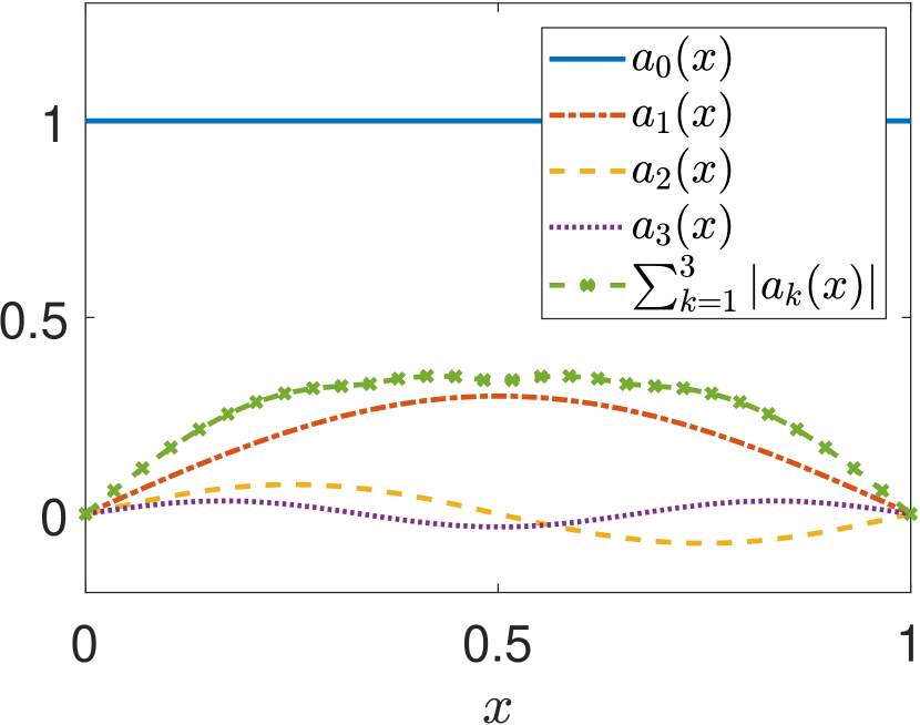
(a) setting 1

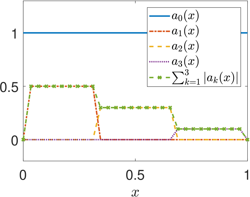
(b) setting 2

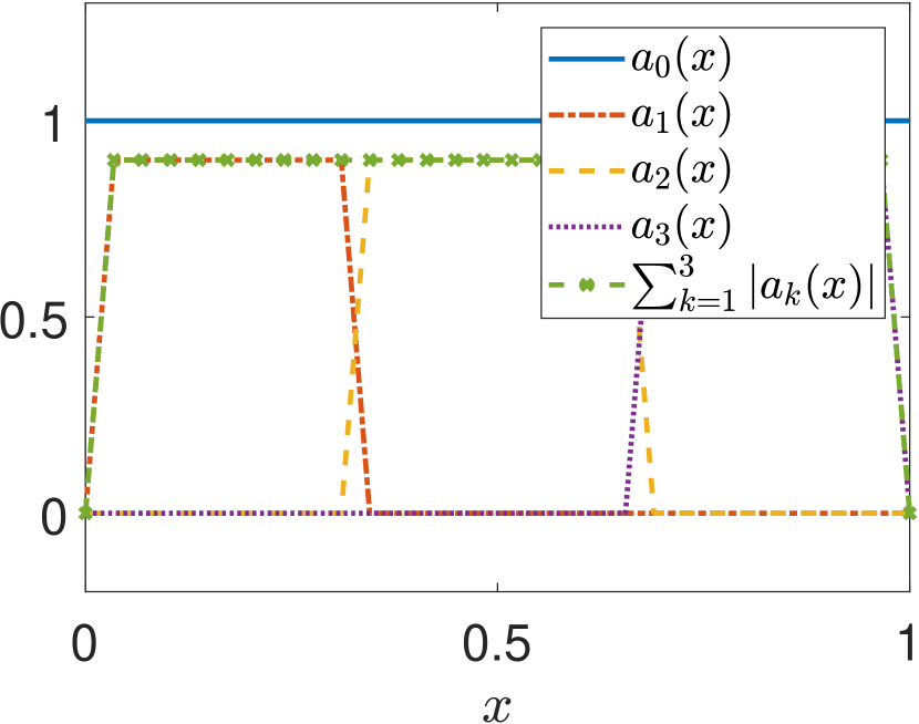
(c) setting 3

Figure 1: Functions $a_{k}(x)$, $k=1,\ldots,K$, for the settings from Table 2.

Table 2: Problem setting, one-dimensional problems.

setting	$a_{0}({x})$	$a_{1}({x})$	$a_{2}({x})$	$a_{3}({x})$	$\mu$	$\mu_{\text{class}}$
1	$1$	$\frac{0.3}{1^{2}}\sin(1\pi x)$	$\frac{0.3}{2^{2}}\sin(2\pi x)$	$\frac{0.3}{3^{2}}\sin(3\pi x)$	0.35	0.41
2	$1$	$0.5\chi_{(0,1/3)}$	$0.3\chi_{(1/3,2/3)}$	$0.1\chi_{(2/3,1)}$	0.5	0.9
3	$1$	$0.95\chi_{(0,1/3)}$	$0.95\chi_{(1/3,2/3)}$	$0.95\chi_{(2/3,1)}$	0.95	2.85

We apply the mean-based preconditioning, see Section 4.1, to each of the settings. We compute the true extreme eigenvalues of the resulting preconditioned matrices, the theoretical spectral bounds $\underline{c}$ and $\overline{c}$ given by Lemma 4.2 and Corollary 4.4, and the classical spectral bounds

(111) $$\underline{c}_{\rm class}=1-\mu_{\rm class}\lambda_{\rm max}(\psi_{s}),\quad\overline{c}_{\rm class}=1+\mu_{\rm class}\lambda_{\rm max}(\psi_{s}).$$

derived, e.g., in [24, Theorem 3.8]. The roots of the Legendre orthogonal polynomials are obtained from [21]. The results for complete polynomials are summarized in Table 3. For all considered settings, we obtained

(112) $$\underline{c}_{\rm class}\leq\underline{c}\leq\lambda_{\rm min}(\bm{M}^{-1}\bm{A})\leq\lambda_{\rm max}(\bm{M}^{-1}\bm{A})\leq\overline{c}\leq\overline{c}_{\rm class}.$$

Moreover, for the third setting, the classical bounds do not provide any useful information because $\mu_{\rm class}\lambda_{\rm max}(\psi_{s})>1$, and thus $\underline{c}_{\rm class}<0$.

Table 3: Mean-based preconditioning and complete polynomials: a comparison of the new and the classical spectral bounds, and the extreme eigenvalues of the preconditioned matrix for the three different settings from Table 2.

	$s-1$	${\color[rgb]{0,0,0}\kappa(\bm{A})}$	$\underline{c}_{\rm class}$	$\underline{c}$	$\lambda_{\rm min}(\bm{M}^{-1}\bm{A})$	$\lambda_{\rm max}(\bm{M}^{-1}\bm{A})$	$\overline{c}$	$\overline{c}_{\rm class}$	$\overline{c}/\underline{c}$	$\overline{c}_{\rm class}/\underline{c}_{\rm class}$
setting 1	1	458.42	0.76	0.80	0.83	1.17	1.20	1.24	1.51	1.62
	2	498.47	0.68	0.73	0.76	1.24	1.27	1.32	1.75	1.92
	…
	6	546.55	0.61	0.67	0.69	1.31	1.33	1.39	2.00	2.26
	7	550.80	0.61	0.66	0.68	1.32	1.34	1.39	2.02	2.29
setting 2	1	542.75	0.48	0.71	0.71	1.29	1.29	1.52	1.81	3.16
	2	629.41	0.30	0.61	0.61	1.39	1.39	1.70	2.26	5.60
	…
	6	739.40	0.15	0.53	0.53	1.47	1.47	1.85	2.81	12.72
	7	749.57	0.14	0.52	0.52	1.48	1.48	1.86	2.85	13.73
setting 3	1	947.79	-0.65	0.45	0.45	1.56	1.56	2.65	3.43	-
	2	1596.34	-1.21	0.26	0.26	1.74	1.74	3.21	6.57	-
	…
	6	4576.93	-1.71	0.10	0.10	1.90	1.90	3.71	19.34	-
	7	5294.63	-1.74	0.09	0.09	1.91	1.91	3.74	21.80	-

Next, we consider a two-dimensional problem in $D=[0,1]^{2}$ with homogeneous Dirichlet boundary conditions, uniform mesh with $N_{\rm elem}=20^{2}=400$ elements, uniform distributions of $\xi_{k}$, $k=1,\ldots,K$, with images in $[-1,1]$. The approximation and test spaces are spanned by a tensor product of continuous piece-wise bilinear functions defined on $D$ and of $K$-variate Legendre polynomials. We define two different settings for $a_{k}({\bm{x}})$, $k=0,\ldots,K$, see Table 4, which are analogously as before considered constant on every element. For both settings, we investigate the spectral bounds for the splitting-based preconditioning (SB) and the two-by-two block Gauss-Seidel preconditioning (GS2). The results are shown in Tables 5 and 6. According to Remark 4.18, the upper bound of $\kappa(\bm{M}_{\rm GS2}^{-1}\bm{A})$ is obtained as $1/d_{t}$. The values of $t$ used in Lemma 4.14 for obtaining $\underline{c}$ and $\overline{c}$ are presented.

Table 4: Problem setting, two-dimensional problems.

setting	$a_{0}({x_{1},x_{2}})$	$a_{1}({x_{1},x_{2}})$	$a_{2}({x_{1},x_{2}})$	$a_{3}({x_{1},x_{2}})$	$\mu$
4	$1$	${0.3}\sin(1\pi x_{1})$	${0.3}\sin(2\pi x_{2})$	${0.3}\sin(2\pi x_{1})$	0.83

setting	$a_{0}({x_{1},x_{2}})$	$a_{2k+1}(x_{1},x_{2})$	$a_{2k+2}(x_{1},x_{2})$
5	$1$	$\frac{0.9}{K}\sin\left((k+1)\pi x_{1}\right)$	$\frac{0.9}{K}\sin\left((k+1)\pi x_{2}\right)$

Table 5: Splitting-based and two-by-two block Gauss-Seidel preconditioning for complete polynomials. Results for setting 4 (Table 4), $K=3$, polynomial degree $s-1=1,\dots,5$.

$s-1$	$\kappa(\bm{A})$	$\kappa(\bm{M}_{\rm SB}^{-1}\bm{A})$	$\overline{c}/\underline{c}$	$\kappa(\bm{M}_{\rm GS2}^{-1}\bm{A})$	$1/d_{t}$	$t$
1	265.65	1.76	2.83	1.08	1.30	2
2	334.62	2.13	2.90	1.15	1.31	3
3	384.58	2.36	2.90	1.20	1.31	3
4	420.15	2.50	2.90	1.22	1.31	3
5	446.06	2.56	2.90	1.24	1.31	3

Table 6: Splitting-based and two-by-two block Gauss-Seidel preconditioning for complete polynomials. Results for setting 5 (Table 4), polynomial degree $s-1=2$, expansion length $K=1,\dots,7$.

$K$	$\kappa(\bm{A})$	$\kappa(\bm{M}_{\rm SB}^{-1}\bm{A})$	$\overline{c}/\underline{c}$	$\kappa(\bm{M}_{\rm GS2}^{-1}\bm{A})$	$1/d_{t}$	$t$	$\mu$
1	580.00	3.36	3.38	1.41	1.42	3	0.90
2	437.88	2.74	3.38	1.28	1.42	3	0.90
3	334.62	2.13	2.90	1.15	1.31	3	0.83
4	293.51	1.88	2.70	1.10	1.27	3	0.79
5	272.26	1.73	2.59	1.08	1.24	2	0.77
6	258.72	1.63	2.52	1.06	1.23	2	0.75
7	247.96	1.56	2.48	1.05	1.22	2	0.74

5 Conclusion

We introduced a new tool for obtaining guaranteed and two-sided spectral bounds for discretized stochastic Galerkin problems preconditioned by a matrix with modified stochastic part from the spectral information of certain small matrices, from which the large stochastic Galerkin matrix is constructed. Moreover, this analysis only requires point-wise or local dominance of the deterministic part of the expansion of the parameter-dependent function $a(\bm{x},\bm{\xi})$, represented here by the parameter $\mu$, while the standard bounds are typically based on the absolute global dominance. The derived estimates are therefore also applicable to problems where global dominance is not achieved. We showed for three types of block-diagonal preconditioners, including less standard ones, how this technique is used to obtain spectral bounds depending solely on $\mu$ and the properties of the stochastic approximation space (here classical orthogonal polynomials). From the locality of $\mu$, it also follows that the obtained bounds are tighter than the classical ones. Similar ideas based on local properties of a preconditioner appear also in [16].

References

- [1] M. Ainsworth and J. T. Oden, A Posteriori Error Estimation in Finite Element Analysis, John Wiley & Sons, 2000.
- [2] O. Axelsson, Iterative solution methods, Cambridge University Press, 1996.
- [3] I. Babuška, F. Nobile, and R. Tempone, A stochastic collocation method for elliptic partial differential equations with random input data, SIAM review, 52 (2010), pp. 317–355.
- [4] I. Babuška, R. Tempone, and G. E. Zouraris, Galerkin finite element approximations of stochastic elliptic partial differential equations, SIAM Journal on Numerical Analysis, 42 (2004), pp. 800–825.
- [5] A. Bespalov, C. E. Powell, and D. Silvester, Energy norm a posteriori error estimation for parametric operator equations, SIAM Journal on Scientific Computing, 36 (2014), pp. A339–A363.
- [6] A. J. Crowder and C. E. Powell, CBS constants & their role in error estimation for stochastic Galerkin finite element methods, Journal of Scientific Computing, 77 (2018), pp. 1030–1054.
- [7] A. J. Crowder, C. E. Powell, and A. Bespalov, Efficient adaptive multilevel stochastic Galerkin approximation using implicit a posteriori error estimation, arXiv eprint, arXiv:1806.05987, (2018).
- [8] M. Eigel, C. J. Gittelson, C. Schwab, and E. Zander, Adaptive stochastic Galerkin FEM, Computer Methods in Applied Mechanics and Engineering, 270 (2014), pp. 247–269.
- [9] M. Eigel and C. Merdon, Local equilibration error estimators for guaranteed error control in adaptive stochastic higher-order Galerkin finite element methods, SIAM/ASA Journal on Uncertainty Quantification, 4 (2016), pp. 1372–1397.
- [10] M. Eigel, M. Pfeffer, and R. Schneider, Adaptive stochastic Galerkin FEM with hierarchical tensor representations, Numerische Mathematik, 136 (2017), pp. 765–803.
- [11] V. Eijkhout and P. Vassilevski, The role of the strengthened CBS-inequality in multi-level methods, SIAM Review, 33 (1991), pp. 405–419.
- [12] H. Elman and D. Furnival, Solving the stochastic steady-state diffusion problem using multigrid, IMA Journal of Numerical Analysis, 27 (2007), pp. 675–688.
- [13] O. G. Ernst, C. E. Powell, D. J. Silvester, and E. Ullmann, Efficient solvers for a linear stochastic Galerkin mixed formulation of diffusion problems with random data, SIAM Journal on Scientific Computing, 31 (2009), pp. 1424–1447.
- [14] O. G. Ernst and E. Ullmann, Stochastic Galerkin matrices, SIAM Journal on Matrix Analysis and Applications, 31 (2010), pp. 1848–1872.
- [15] W. Gautschi, Orthogonal Polynomials, Computation and Approximation, Oxford University Press, 2004.
- [16] T. Gergelits, K.-A. Mardal, B. F. Nielsen, and Z. Strakoš, Laplacian preconditioning of elliptic PDEs: Localization of the eigenvalues of the discretized operator, SIAM Journal on Numerical Analysis, (to appear).
- [17] A. Khan, A. Bespalov, C. E. Powell, and D. J. Silvester, Robust a posteriori error estimation for stochastic Galerkin formulations of parameter-dependent linear elasticity equations, arXiv eprint, arXiv:1810.07440, (2018).
- [18] J. Kraus and S. Margenov, Robust Algebraic Multilevel Methods and Algorithms, vol. 5, Walter de Gruyter GmbH & Co. KG, Berlin, Radon Series on Computational and Applied Mathematics, 2009.
- [19] A. J. Laub, Matrix Analysis for Scientists and Engineers, SIAM, 2005.
- [20] J. Liesen and Z. Strakoš, Krylov subspace methods, Numerical Mathematics and Scientific Computation, Oxford University Press, Oxford, 2013.
- [21] A. N. Lowan, N. Davids, and A. Levenson, Table of the zeros of the Legendre polynomials of order 1-16 and the weight coefficients for Gauss’ mechanical quadrature formula, Bull. Amer. Math. Soc., 48 (1942), pp. 739–743.
- [22] G. Meurant, A review on the inverse of symmetric tridiagonal and block tridiagonal matrices, SIAM Journal on Matrix Analysis and Applications, 13 (1992), pp. 707–728.
- [23] C. Müller, S. Ullmann, and J. Lang, A Bramble-Pasciak conjugate gradient method for discrete Stokes equations with random viscosity, arXiv eprint, arXiv:1801.01838, (2018).
- [24] C. E. Powell and H. C. Elman, Block-diagonal preconditioning for spectral stochastic finite-element systems, IMA Journal of Numerical Analysis, 29 (2009), pp. 350–375.
- [25] C. E. Powell, D. Silvester, and V. Simoncini, An efficient reduced basis solver for stochastic Galerkin matrix equations, SIAM Journal on Scientific Computing, 39 (2017), pp. A141–A163.
- [26] C. E. Powell and E. Ullmann, Preconditioning stochastic Galerkin saddle point systems, SIAM Journal on Matrix Analysis and Applications, 31 (2010), pp. 2813–2840.
- [27] I. Pultarová, Adaptive algorithm for stochastic Galerkin method, Applications of Mathematics, 60 (2015), pp. 551–571.
- [28] I. Pultarová, Hierarchical preconditioning for the stochastic Galerkin method: Upper bounds to the strengthened CBS constants, Computers & Mathematics with Applications, 71 (2016), pp. 949–964.
- [29] I. Pultarová, Block and multilevel preconditioning for stochastic Galerkin problems with lognormally distributed parameters and tensor product polynomials, International Journal for Uncertainty Quantification, 7 (2017), pp. 441–462.
- [30] E. Rosseel and S. Vandewalle, Iterative solvers for the stochastic finite element method, SIAM J. Sci. Comput., 32 (2010), pp. 372–397.
- [31] B. Sousedík and R. Ghanem, Truncated hierarchical preconditioning for the stochastic Galerkin FEM, International Journal for Uncertainty Quantification, 4 (2014), pp. 333–348.
- [32] B. Sousedík, R. G. Ghanem, and E. T. Phipps, Hierarchical Schur complement preconditioner for the stochastic Galerkin finite element methods: Dedicated to Professor Ivo Marek on the occasion of his 80th birthday., Numerical Linear Algebra with Applications, 21 (2014), pp. 136–151.
- [33] W. Subber and S. Loisel, Schwarz preconditioners for stochastic elliptic PDEs, Computer Methods in Applied Mechanics and Engineering, 272 (2014), pp. 34–57.
- [34] G. Szegő, Orthogonal Polynomials, vol. 23, American Mathematical Society, 3rd ed., 1975.
- [35] E. Ullmann, A Kronecker product preconditioner for stochastic Galerkin finite element discretizations, SIAM Journal on Scientific Computing, 32 (2010), pp. 923–946.
- [36] D. Xiu, Numerical Methods for Stochastic Computations, Princeton University Press, 2010.