Restricted Boltzmann Machine Assignment Algorithm:
Application to solve many-to-one matching problems on weighted bipartite graph

Abstract

In this work an iterative algorithm based on unsupervised learning is presented, specifically on a Restricted Boltzmann Machine (RBM) to solve a perfect matching problem on a bipartite weighted graph. Iteratively is calculated the weights $w_{ij}$ and the bias parameters $\theta=(a_{i},b_{j})$ that maximize the energy function and assignment element $i$ to element $j$. An application of real problem is presented to show the potentiality of this algorithm.

Keywords Optimization  $\cdot$ Combinatorial $\cdot$ Matching  $\cdot$ Assignment Problems  $\cdot$ Neural Networks  $\cdot$ Unsupervised learning  $\cdot$ Restricted Boltzmann Machine

1 Introduction

The assignment problems fall within the combinatorial optimization problems, the problem of matching on a bipartite weighted graph is one of the major problems faced in this compound. Numerous resolution methods and algorithms have been proposed in recent times and many have provided important results, among them for example we find: Constructive heuristics, Meta-heuristics, Approximation algorithms, Iper-heuristics, and other methods. Combinatorial optimization deals with finding the optimal solution between the collection of finite possibilities. The finished set of possible solutions. The heart of the problem of finding solutions in combinatorial optimization is based on the efficient algorithms that present with a polynomial computation time in the input dimension. Therefore, when dealing with certain combinatorial optimization problems one must ask with what speed it is possible to find the solutions or the optimal problem solution and if it is not possible to find a resolution method of this type, which approximate methods can be used in polynomial computational times that lead to stable explanations. Solve this kind of problem in polynomial time $o(n)$ has long been the focus of research in this area until Edmonds [1] developed one of the most efficient methods. Over time other algorithms have been developed, for example the fastest of them is the Micali e Vazirani algorithm [2], Blum [3] and Gabow and Tarjan [4]. The first of these methods is an improvement on that of Edmonds, the other algorithms use different logics, but all of them with computational time equal to $o(m\sqrt{n})$. The problem is fundamentally the following: we imagine a situation in which respect for the characteristics detected on a given phenomenon is to be assigned between elements of two sets, as for example in one of the most known problems such as the tasks and the workers to be assigned to them. A classical maximum cardinality matching algorithm to take the maximum weight range and assign it, in a decision support system, through the domain expert this could also be acceptable, but in a totally automatic system like a system could be of artificial intelligence that puts together pairs of elements on the basis of some characteristics, this way would not be very reliable, totally removing the user’s control. Another problem related to this kind of situation is that of features. Let’s take as an example a classic problem of flight-gate assignment in an airport, on the basis of the history we could have information about the flight, the gates and the time, the flight number and maybe the airline. Little information that even through the best of feature enginering would lead to a model of machine learning, specifically of classification, very poor in information. Treating the same problem with classical optimization, as done so far, would lead to solving it with a perfect matching of maximum weight, and we would return to the beginning.

2 Matching problems

Matching problems are among the fundamental problems in combinatorial optimization. In this set of notes, we focus on the case when the underlying graph is bipartite. We start by introducing some basic graph terminology. A graph $G=(V,E)$ consists of a set $V=A\cup B$ of vertices and a set $E$ of pairs of vertices called edges. For an edge $e=(u,v)$, we say that the endpoints of e are $u$ and $v$; we also say that $e$ is incident to $u$ and $v$. A graph $G=(V,E)$ is bipartite if the vertex set $V$ can be partitioned into two sets $A$ and $B$ (the bipartition) such that no edge in $E$ has both endpoints in the same set of the bipartition. A matching M is a collection of edges such that every vertex of $V$ is incident to at most one edge of $M$. If a vertex $v$ has no edge of $M$ incident to it then $v$ is said to be exposed (or unmatched). A matching is perfect if no vertex is exposed; in other words, a matching is perfect if its cardinality is equal to $|A|=|B|$. In the literature several examples of the real world have been treated such as the assignment of children to certain schools [5], or as donors and patients [6] and workers at companies [7]. The problem of the weighted bipartite matching finds the feasible match with the maximum available weight. This problem was developed in several areas, such as in the work of [8] about protein and structure alignment, or within the computer vision as documented in the work of [9] or as in the paper by [10] in which the similarity of the texts is estimated. Other jobs have faced this problem in the classification [11],[12] e [13], but not for many to one correspondence. The mathematical formulation can be solved by presenting it as a linear program. Each edge $(i,j)$, where $i$ is in $A$ and $j$ is in $B$, has a weight $w_{ij}$. For each edge $(i,j)$ we have a decision variable

$$x_{ij}=\begin{cases}1&\mbox{if the edge is contained in the matching}\\ 0&\mbox{otherwise}\end{cases}$$ (1)

and $x_{ij}\in\mathbb{Z}{\text{ for }}i,j\in A,B$, and we have the following LP:

$$\underset{x_{ij}}{\text{max}}\sum_{(i,j)\in A\times B}w_{ij}x_{ij}$$ (2)

$$\sum_{j\in B}x_{ij}=1{\text{ for }}i\in A$$ (3)

$$\sum_{i\in A}x_{ij}=1{\text{ for }}j\in B$$ (4)

$$0\leq x_{ij}\leq 1{\text{ for }}i,j\in A,B$$ (5)

$$x_{ij}\in\mathbb{Z}{\text{ for }}i,j\in A,B$$ (6)

Figure 1: Bipartite Weighted Matching

3 Motivation

The problem in a weighted bipartite graph $G=(V=A\cup B,W)$, is when we have different weights (historical data) $W=\left(w_{11},w_{12}...,w_{ij}\right)$ for the set of nodes to which corresponds the same set of nodes $B$. One of most popular solution is Hungarian algorithm [16] . The assignment rule therefore in many real cases could be misleading and limiting as well as it could be unrealistic as a solution. Machine learning (ML) algorithms are increasingly gaining ground in applied sciences such as engineering, biology, medicine, etc. both supervised and unsupervised learning models. The matching problem in this case can be seen as a set of inputs $x_{1},...,x_{k}$ (in our case the nodes of the set A) and a set of ouput $y_{1},...,y_{k}$ (the respective nodes of the set $B$), weighed by a series of weights $w_{11},...w_{ij}$, which inevitably recall the structure of a classic neural network. The problem is that in this case there would be a number of classes (in the case of assignment) equal to the number of inputs. Considering it as a classic machine learning problem, the difficulty would lie in the features and their engineering, on the one hand, while on the other the number of classes to predict (assign) would be very large. For example, if we think about matching applicants and jobs, if we only had the name of a candidate for the job, we would have very little info to build a robust machine learning model, and even a good features engineering would not lead to much, but having available other information on the candidate they could be extracted it is used case never as "weight" to build a neural network, but even in this case the constraint of a classic optimization model solved with ML techniques would not be maintained, let’s say we would "force" a little hand. While what we want to present in this work is the resolution of a classical problem of matching (assignment) through the application of a ML model, in this case of a neural network, which as already said maintains the mathematical structure of a node (input) and arc (weight) but instead of considering the output of arrival (the set $B$) as classification label (assignment) in this case we consider an unsupervised neural network, specifically an Restricted Boltzmann Machine.

4 Contributions

The contributions of this work are mainly of two types: the first is related to the ability to use an unsupervised machine learning model to solve a classical optimization problem which in turn has the mathematical structure of a neural network based on two layers, in our case of RBM a visible and a hidden one. In this case the nodes of the set $B$ become the variables of the model and the number of times that the node $i$ has been assigned to the node $j$ (for example in problems that concerns historical data analysis), becomes the weight $w_{ij}$ which at its turn becomes the value of the variable $i$-th in the RBM model. The second is the ability to solve real problems, as we will see later in the article, in which it is necessary to carry out a matching between elements of two sets and the maximum weight span is not said to be the best assignment, especially in the case where the problem is many-to-one, like many real problems.

5 Restricted Boltzmann Machine

Restricted Boltzmann Machine is an unsupervised method neural networks based [14]; the algorithm learns one layer of hidden features. When the number of hidden units is smaller than that of visual units, the hidden layer can deal with nonlinear complex dependency and structure of data, capture deep relationship from input data , and represent the input data more compactly. Assuming there are $c$ visible units and $m$ hidden units in an Restricted Boltzmann Machine. So $v_{i}$ for $i=1,...,c$ indicates the state of the $i-$th visible unit, where

$$v_{i}=\begin{cases}1&\mbox{if the i-th term is annotated to the element }\\ 0&\mbox{otherwise}\end{cases}$$ (7)

for $i=1,...,c$ and furthemore we have

$$h_{j}=\begin{cases}1&\mbox{the state of hidden unit is active}\\ 0&\mbox{otherwise}\end{cases}$$ (8)

for $j=1,...,m$ and $w_{ij}$ is the weight associated with the connection between $v_{i}$ and $h_{j}$ and define also the joint configuration $(v,h)$.

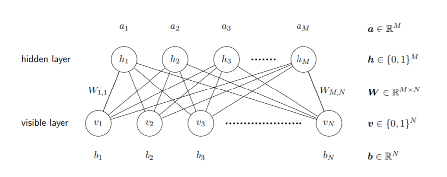
Figure 2: Restricted Boltzamann Machine Structures

The energy function that capturing the interaction patterns between visible layer and hidden layer is define as follow:

$$E(v,h|\theta)=-\sum_{i=1}^{c}a_{i}v_{i}-\sum_{j=1}^{m}b_{j}h_{j}-\sum_{i=1}^{c}\sum_{j=1}^{m}v_{i}h_{j}w_{ij}$$ (9)

where $\theta=\left(w_{ij},a_{i},b_{j}\right)$ are parameters of the model: $a_{i}$ and $b_{j}$ are biases for the visible and hidden variables, respectively. The parameters $w_{ij}$ is the weights of connection between visible variables and hidden variables. The joint probability is represented by the follow quantity:

$$p(v,h)=\frac{e^{-}E(v,h)}{Z}$$ (10)

where

$$Z=\sum_{v,h}e^{-E(v,h)}$$

is a normalization constant and the conditional distributions over the visible and hidden units are given by sigmoid functions as follows:

$$p(v_{i}=1|h)=\sigma\left(\sum_{j=1}^{m}w_{ij}h_{j}+a_{i}\right)$$ (11)

$$p(h_{j}=1|v)=\sigma\left(\sum_{i=1}^{c}w_{ij}v_{i}+b_{j}\right)$$ (12)

where $\sigma=\frac{1}{1+e^{-x}}$

RBM are trained to optimizie the product of probabilities assigned to some training set $V$ (a matrix, each row of which is treated as a visible vector v)

$$\underset{w_{ij}}{\text{arg}\ \text{max}}\prod_{i=1}^{c}p(v_{i})$$ (13)

The RBM training takes place through the Contrastive Divergence Algorithm (see Hinton 2002 [15]). For the (4) and (7) we can pass to log-likelihood formulation

$$L_{v}=log\sum_{h}e^{-E(v,h)}-log\sum_{v,h}e^{-E(v,h)}$$ (14)

and derivate the quantity

$$\frac{\partial L_{v}}{\partial w_{ij}}=\sum_{h}p(h|v)\cdot v_{i}h_{j}-\sum_{v,h}p(v,h)\cdot v_{i}h_{j}$$ (15)

$$\frac{\partial L_{v}}{\partial w_{ij}}=\mathbb{E}[p(h|v)]-\mathbb{E}[p(v,h)]$$ (16)

In the above expression, the first quantity represents the expectation of $v_{i}\cdot h_{j}$ to the conditional probability of the hidden states given the visible states and the second term represents the expectation of $v_{i}\cdot h_{j}$ to the joint probability of the visible and hidden states. In order to maximize the (7), which involves log of summation, there is no analytical solution and will use the stochastic gradient ascent technique. In order to compute the unknown values of the weights $w_{ij}$ such that they maximize the above likelihood, we compute using gradient ascent :

$$w_{ij}^{k+1}=w_{ij}^{k}+\alpha\cdot\frac{\partial L_{v}}{\partial w_{ij}}$$

where $\alpha\in(0,1)$ is the learning rate. At this formulation we can add an term of penality and obtain the follow

$$w_{ij}^{k+1}=w_{ij}^{k}+\alpha\cdot\frac{\partial L_{v}}{\partial w_{ij}}+\eta\cdot\frac{w_{ij}^{k-1}}{w_{ij}^{k}}$$ (17)

where $\eta>0$ is penalty parameters and $\eta\cdot\frac{w_{ij}^{k-1}}{w_{ij}^{k}}$ measure the contribute of weights variation in the $k$-th step of update.

6 Restricted Boltzmann Machine Assignment Algorithm (RBMAA)

In this section is presented the algorithm RBM based and is explaneid the single steps.

1. In this step the algorithm takes as input the matrix $W$ relative to the weights of the assignments, either the weight $w_{ij}$ represents the number of times that the element $i$ has been assigned to the element $j$
   

2. The matrix $W$ is binarized. For each element $w_{ij}>$ 0 take 1 or 0 and an a matrix $\tilde{W}$ is created with elements 0-1.
   

3. In this step the RBM is applied taking as input the binary matrix $\tilde{W}$. The probability product related to the visible units of the RBM is maximized (13). The weights $w_{ij}$ are updated according to (17) and the biases according to the RBM training rule. Once these updated values are obtained, the optimized value $\hat{p}(v_{i})$ if this is greater than $\epsilon>$ 0 assigns 1 otherwise 0 and the iteration of the RBM is restarted until for each row of the matrix there is not a single value 1 which is the same as assignment. The quantile of level $\alpha=$ 0.99 was used to determine the threshold $\epsilon$.
   

4. The output of the algorithm is a matrix with values 0-1 and on each line we obtain a single value equal to 1 which is equivalent to the assignment of the element $i$ to the element $j$.

The pseudocode is presented in the next section.

1 Input:

$\epsilon$, threshold value

$b_{j}$, hidden units bias value

$a_{i}$, visible units bias value

$\alpha$, learning rate for visible bias updating

$\beta$, learning rate for hidden bias updating

Matrix $n\times m$, $W=\{w_{ij}\}$ number of times which $i$ has been assigned to $j$ 

 

2Binarize $W$ to get $\dot{W}=\{\dot{w}_{ij}\}\in[0,1]$

foreach $\text{i}\ in\ W$ do

       if $w_{ij}>0$  then

             1

            

            

      else

             0

            

      

3while $\sum_{i=1}^{c}\hat{w}_{ij}\neq$ 1 do

       

      $\underset{\dot{w}_{ij}}{\text{arg}\ \text{max}}\prod_{i=1}^{c}p(v_{i})$

       Update $w_{ij}$, $w_{ij}^{k+1}=w_{ij}^{k}+\alpha\cdot\frac{\partial L_{v}}{\partial w_{ij}}$

      Update $b_{j}$, $b_{j}^{k+1}=b_{j}^{k}+\beta\cdot\frac{\partial L_{v}}{\partial b_{j}}$

      Update $a_{i}$, $a_{i}^{k+1}=a_{i}^{k}+\alpha\cdot\frac{\partial L_{v}}{\partial a_{i}}$

      if $\hat{p}(v_{i})>\epsilon$ then

            1

            

            

      else

             0

            

      

4Output: Matrix $n\times m$, $\hat{P}=\{0,1\}$ such that $\sum_{i}\hat{p}_{ij}=1$, $\forall i\in A$

Algorithm 1 Restricted Boltzmann Assignment

7 Application of the RBMAA to a real problem

Now we proceed to provide the results of the application of the algorithm (see Appendix). The problem instance is 351 elements for the set $A$ and 35 for the set $B$; the goal is to assign for each element of $A$, one and only one element of $B$, so as to have the sum for row equal to 1 as in (3) and in step 4 of the algorithm. The weights $w_{ij}$ are represented by the number of times the element $a_{i}\in A$ has been assigned to the element $b_{j}\in B$, based on a set of historical data that we have relative to flight-gate assignments of a well-known international airport. The difficulty is the one discussed in the first part of the work, in which we want to obtain a robust machine learning algorithm that classifies and assigns the respective gate for each flight. Starting from the available features, the algorithm presented in the work was implemented. The computational results are very interesting in terms of calculation speed and assignment.

8 Conclusions and discussion

This can be the starting point for more precise, fast and sophisticated algorithms, which combine the combinatorial optimization with machine learning but on the basis of unsupervised learning and not only on the optimization of cost functions.

9 Appendix

Node1

Node2

Node1

Node2

Node1

Node2

Node1

Node2

Node1

Node2

Node1

Node2

Node1

Node2

A2

B1

A173

B5

A203

B10

A268

B15

A158

B20

A48

B25

A183

B30

A72

B1

A208

B5

A238

B10

A303

B15

A193

B20

A83

B25

A218

B30

A107

B1

A243

B5

A308

B10

A338

B15

A228

B20

A93

B25

A253

B30

A117

B1

A278

B5

A318

B10

A22

B16

A263

B20

A118

B25

A288

B30

A142

B1

A313

B5

A343

B10

A57

B16

A273

B20

A153

B25

A323

B30

A177

B1

A348

B5

A27

B11

A92

B16

A298

B20

A188

B25

A7

B31

A212

B1

A32

B6

A75

B11

A127

B16

A333

B20

A223

B25

A42

B31

A247

B1

A67

B6

A97

B11

A162

B16

A17

B21

A258

B25

A77

B31

A282

B1

A102

B6

A110

B11

A197

B16

A52

B21

A293

B25

A147

B31

A292

B1

A137

B6

A132

B11

A232

B16

A87

B21

A328

B25

A182

B31

A317

B1

A172

B6

A202

B11

A267

B16

A122

B21

A12

B26

A217

B31

A1

B2

A207

B6

A237

B11

A302

B16

A157

B21

A47

B26

A252

B31

A11

B2

A242

B6

A307

B11

A337

B16

A167

B21

A82

B26

A287

B31

A36

B2

A277

B6

A342

B11

A21

B17

A192

B21

A152

B26

A322

B31

A71

B2

A312

B6

A26

B12

A56

B17

A227

B21

A187

B26

A6

B32

A106

B2

A347

B6

A61

B12

A91

B17

A262

B21

A257

B26

A41

B32

A141

B2

A31

B7

A74

B12

A161

B17

A272

B21

A270

B26

A76

B32

A176

B2

A66

B7

A96

B12

A196

B17

A297

B21

A327

B26

A146

B32

A211

B2

A101

B7

A131

B12

A231

B17

A332

B21

A46

B27

A181

B32

A246

B2

A111

B7

A166

B12

A266

B17

A16

B22

A81

B27

A216

B32

A256

B2

A136

B7

A201

B12

A301

B17

A51

B22

A116

B27

A251

B32

A281

B2

A171

B7

A236

B12

A336

B17

A86

B22

A151

B27

A321

B32

A316

B2

A206

B7

A271

B12

A20

B18

A121

B22

A186

B27

A5

B33

A35

B3

A241

B7

A306

B12

A55

B18

A156

B22

A221

B27

A40

B33

A70

B3

A276

B7

A341

B12

A90

B18

A191

B22

A291

B27

A85

B33

A105

B3

A286

B7

A351

B12

A125

B18

A226

B22

A326

B27

A120

B33

A140

B3

A311

B7

A25

B13

A135

B18

A261

B22

A10

B28

A145

B33

A175

B3

A346

B7

A60

B13

A160

B18

A296

B22

A45

B28

A155

B33

A210

B3

A30

B8

A95

B13

A170

B18

A331

B22

A80

B28

A180

B33

A280

B3

A65

B8

A130

B13

A195

B18

A15

B23

A115

B28

A215

B33

A315

B3

A100

B8

A165

B13

A230

B18

A50

B23

A150

B28

A250

B33

A350

B3

A205

B8

A200

B13

A240

B18

A62

B23

A185

B28

A320

B33

A34

B4

A275

B8

A245

B13

A265

B18

A190

B23

A220

B28

A4

B34

A69

B4

A285

B8

A305

B13

A300

B18

A225

B23

A255

B28

A39

B34

A104

B4

A310

B8

A340

B13

A335

B18

A235

B23

A290

B28

A109

B34

A139

B4

A345

B8

A37

B14

A19

B19

A260

B23

A325

B28

A144

B34

A174

B4

A29

B9

A59

B14

A89

B19

A295

B23

A9

B29

A179

B34

A209

B4

A64

B9

A94

B14

A124

B19

A330

B23

A44

B29

A214

B34

A222

B4

A99

B9

A129

B14

A159

B19

A14

B24

A54

B29

A249

B34

A244

B4

A112

B9

A164

B14

A194

B19

A24

B24

A79

B29

A284

B34

A254

B4

A134

B9

A199

B14

A229

B19

A49

B24

A114

B29

A319

B34

A279

B4

A169

B9

A234

B14

A239

B19

A84

B24

A149

B29

A3

B35

A314

B4

A204

B9

A269

B14

A264

B19

A119

B24

A184

B29

A38

B35

A349

B4

A274

B9

A339

B14

A299

B19

A154

B24

A219

B29

A73

B35

A33

B5

A309

B9

A23

B15

A334

B19

A189

B24

A289

B29

A108

B35

A68

B5

A28

B10

A58

B15

A344

B19

A224

B24

A324

B29

A143

B35

A103

B5

A63

B10

A128

B15

A18

B20

A259

B24

A8

B30

A178

B35

A113

B5

A98

B10

A163

B15

A53

B20

A294

B24

A43

B30

A213

B35

A138

B5

A133

B10

A198

B15

A88

B20

A304

B24

A78

B30

A248

B35

A148

B5

A168

B10

A233

B15

A123

B20

A329

B24

A126

B30

A283

B35

A13

B25

References

-
[1]
J. Edmonds. "Paths, trees and
flowers". Canadian Journal of Mathematics, 17: 449-467, 1965
-
[2]
S. Micali and V. V. Vazirani. "An algorithm for finding maximum matching in general
graphs". In Proceedings of the twenty First annual IEEE
Symposium on Foundations of Computer Science,1980.
-
[3]
N. Blum. "A new approach to maximum matching in
general graphs". In Proc. 17th ICALP, volume 443 of
Lecture Notes in Computer Science, pages 586 - 597.
Springer-Verlag, 1990.
-
[4]
H. N. Gabow and R. E. Tarjan. "Faster scaling
algorithms for general graph matching problems". J.
ACM, 38(4):815 - 853, 1991.
-
[5]
Ryoji Kurata, Masahiro Goto, Atsushi
Iwasaki, and Makoto Yokoo. "Controlled school choice
with soft bounds and overlapping types". In AAAI Conference
on Artificial Intelligence (AAAI), 2015.
-
[6]
Dimitris Bertsimas, Vivek F Farias,
and Nikolaos Trichakis. "Fairness, efficiency, and flexibility
in organ allocation for kidney transplantation". Operations
Research, 61(1):73–87, 2013.
-
[7]
John Joseph Horton. "The effects of algorithmic
labor market recommendations: evidence from a field
experiment",To appear, Journal of Labor Economics, 2017.
-
[8]
E Krissinel and K Henrick.
"Secondary-structure matching (ssm), a new tool for fast
protein structure alignment in three dimensions". Acta
Crystallographica Section D: Biological Crystallography,
60(12):2256–2268, 2004.
-
[9]
Serge Belongie, Jitendra Malik, and
Jan Puzicha. "Shape matching and object recognition using
shape contexts". IEEE Transactions on Pattern Analysis
and Machine Intelligence, 24(4):509–522, 2002.
-
[10]
Liang Pang, Yanyan Lan, Jiafeng Guo,
Jun Xu, Shengxian Wan, and Xueqi Cheng. "Text matching
as image recognition". In AAAI Conference on Artificial
Intelligence (AAAI), 2016.
-
[11]
Gediminas Adomavicius
and YoungOk Kwon." Improving aggregate recommendation
diversity using ranking-based techniques". IEEE
Transactions on Knowledge and Data Engineering
(TKDE), 24(5):896–911, 2012.
-
[12]
Chaofeng Sha, Xiaowei Wu, and Junyu
Niu. "A framework for recommending relevant and diverse
items". In Proceedings of the International Joint Conference
on Artificial Intelligence (IJCAI), 2016.
-
[13]
Azin Ashkan, Branislav Kveton,
Shlomo Berkovsky, and Zheng Wen. "Optimal greedy
diversity for recommendation". In Proceedings of the
International Joint Conference on Artificial Intelligence
(IJCAI), pages 1742–1748, 2015.
-
[14]
A. Fischer and C. Igel,
"An Introduction to Restricted Boltzmann Machines,
in Progress in Pattern Recognition, Image Analysis,
Computer Vision, and Applications", vol. 7441 of
Lecture Notes in Computer Science, pp. 14–36,
Springer Berlin Heidelberg, Berlin, Heidelberg, 2012.
-
[15]
Hinton, G. E. "A Practical Guide to Training Restricted
Boltzmann Machines". Technical Report, Department of Computer Science, University of Toronto,
2010.
- [16] H.W. Kuhn, "On the origin of the Hungarian method for the assignment problem, in J.K. Lenstra, A.H.G. Rinnooy Kan, A. Schrijver", History of Mathematical Programming, Amsterdam, North-Holland, 1991, pp. 77-81