\end{figure}
A better approach, which combines manageable register requirements with
a more square form of the tile is to subdivide the two smaller loops into tiles
(see Listing~\ref{lst:tsmttsm4} and Figure~\ref{fig:genv8}). This
mapping also allows for much more flexibility, as the tile sizes can
be chosen small enough to avoid spilling or reach a certain occupancy
goal but also large enough to create a high FMA/load ratio. Tile
sizes that are not divisors of the small loop dimensions can be covered
by generating guarding statements for tile entries that could
possibly overlap to only be executed by threads with a tile index that
does not extend beyond the border of the slice. This is helpful for matrix
dimensions that have few divisors, e.g., prime numbers.
\begin{figure} \centering
\includegraphics[scale=0.9]{tsmttsm_mapping4.pdf}
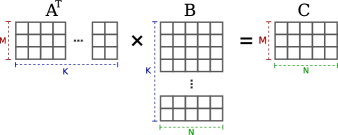
\caption{\emph{TSMTTSM}: Parallelization over $K$ and transposed tiling of the two
inner loops, here with tile size
$2\times3$} \label{fig:genvtransposed}
\end{figure}
Mapping a continuous range of values to a thread leads to strided loads,
which can be detrimental to performance. The same entry in two
consecutive threads’␣partitions␣is␣always␣as␣far␣apart␣as␣the␣tile
side␣length.␣A␣more␣advantageous,␣continuous␣load␣pattern␣can␣be
achieved␣by␣transposing␣the␣threads’ tiles, as shown in Figure
\ref{fig:genvtransposed}. The corresponding values in a tile
are now consecutive.
\subsection{Leap Frogging}
On NVIDIA’s␣GPU␣architectures,␣load␣operations␣can␣overlap␣with␣each␣other.␣The
execution␣will␣only␣stall␣at␣an␣instruction␣that␣requires␣an␣operand␣from␣an
outstanding␣load.␣The␣compiler␣maximizes␣this␣overlap␣by␣moving␣all␣loads␣to␣the
beginning␣of␣the␣loop␣body,␣followed␣by␣the␣floating-point␣(FP)␣instructions␣that
consume␣the␣loaded␣values.␣Usually␣at␣least␣one␣or␣two␣of␣the␣loads␣come␣from
memory␣and␣thus␣take␣longer␣to␣complete␣than␣other␣queued␣loads,␣so␣that
execution␣stalls␣at␣the␣first␣FP␣instruction.␣␣A␣way␣to␣circumvent
this␣stall␣is␣to␣load␣the␣inputs␣one␣loop␣iteration␣ahead␣into␣a␣separate␣set␣of
\emph{next}␣registers,␣while␣the␣computations␣still␣happen␣on␣the␣\emph{current}
values.␣At␣the␣end␣of␣the␣loop,␣the␣\emph{next}␣values␣become␣the␣\emph{current}
values␣of␣the␣next␣loop␣iteration␣by␣assignment.␣These␣assignments␣are␣the␣first
instructions␣that␣depend␣on␣the␣loads␣and␣thus␣the␣computations␣can␣happen␣while
the␣loads␣are␣still␣in␣flight.
\subsection{Global␣Reduction}\label{sec:globred}
After␣each␣thread␣has␣serially␣computed␣its␣partial,␣thread-local
result,␣a␣global␣reduction␣is␣required,␣which␣is␣considered
overhead.␣Its␣runtime␣depends␣only␣on␣the␣thread␣count,␣though,
whereas␣the␣time␣spent␣in␣the␣serial␣summation␣grows␣linearly␣with␣the
row␣count␣and␣therefore␣becomes␣marginal␣for␣large␣row␣counts.
However,␣as␣shown␣by~\cite{jonas_toms},␣the␣performance
at␣small␣row␣counts␣can␣still␣be␣relevant,␣as␣the␣available␣GPU␣memory
may␣be␣shared␣by␣more␣data␣structures␣than␣just␣the␣two␣tall␣\&␣skinny
matrices,␣limiting␣the␣data␣set␣size.
Starting␣with␣the␣\emph{Pascal}␣architecture,␣atomic␣add␣operations␣for␣double
precision␣values␣are␣available␣for␣global␣memory,␣making␣global
reductions␣more␣efficient␣than␣on␣older␣systems.␣␣Each␣thread␣can␣just
use␣an␣\verb|atomicAdd|␣of␣its␣partial␣value␣to␣update␣the␣final␣results.␣The
throughput␣of␣global␣\verb|atomicAdd|␣operations␣is␣limited␣by␣the
amount␣of␣contention,␣which␣grows␣for␣smaller␣matrix␣sizes.␣␣We
improve␣on␣this␣global␣atomic␣reduction␣variant␣with␣a␣local␣atomic
variant␣that␣reduces␣the␣amount␣of␣global␣\verb|atomicAdd|␣operations
by␣first␣computing␣thread-block-local␣partial␣results␣using␣shared
memory␣atomics.␣This␣is␣followed␣by␣a␣global␣reduction␣of␣the␣local
results.␣Additionally,␣we␣opportunistically␣reduce␣the␣amount␣of
launched␣threads␣for␣small␣row␣counts.
\section{TSMM}
\subsection{Thread␣Mapping}
In␣contrast␣to␣the␣\emph{TSMTTSM}␣kernel,␣the␣summation␣is␣done␣along␣the
short␣$M$␣axis,␣with␣no␣need␣for␣a␣global␣reduction.␣Though
the␣short␣sum␣could␣be␣parallelized,␣this␣is␣not␣necessary␣in␣this
case,␣as␣the␣other␣two␣loop␣dimensions␣supply␣sufficient␣parallelism.
The␣visualizations␣in
Figures~\ref{fig:tsmm_mapping_1T}-\ref{fig:tsmm_mapping_u}␣show
slices␣perpendicular␣to␣the␣$M$␣axis,␣since␣this␣dimension␣will
not␣be␣parallelized.
\begin{figure}
␣␣\centering
␣␣\includegraphics[scale=0.5]{tsmm_mapping_1T.pdf}
␣␣\caption{\emph{TSMM}:␣Parallelization␣over␣$K$,␣a␣single␣thread
␣␣␣␣computes␣a␣full␣result␣row␣of␣$\BM$.␣Slice␣perpendicular␣to␣the
␣␣␣␣$M$␣axis,␣the␣(long)␣$K$␣axis␣extends␣“indefinitely’’␣on␣both
␣␣␣␣sides.}␣\label{fig:tsmm_mapping_1T}
\end{figure}
The␣first␣option␣is␣to␣only␣parallelize␣over␣the␣long␣$K$␣dimension␣as
shown␣in␣Figure~\ref{fig:tsmm_mapping_1T}.␣Each␣entry␣in␣$\AM$
would␣be␣loaded␣once␣and␣then␣reused␣out␣of␣a␣register.␣The␣$N$␣sums
that␣each␣thread␣computes␣require␣a␣$2N$␣registers,␣which
is␣not␣a␣prohibitive␣number␣even␣at␣$N=64$␣but␣still␣does
reduce␣occupancy.␣A␣more␣severe␣disadvantage␣are␣the␣strided␣stores.␣␣As
each␣thread␣produces␣and␣stores␣a␣full␣row␣of␣$\BM$,␣the␣addresses
stored␣to␣by␣the␣different␣threads␣are␣far␣apart,␣leading␣to␣partially
written␣cache␣lines.␣␣This␣in␣turn␣causes␣a␣write-allocate␣read
stream␣of␣the␣result␣matrix␣$\BM$␣to␣ensure␣fully␣consistent␣cache
lines,␣thereby␣reducing␣the␣arithmetic␣intensity␣of␣the␣kernel.
This␣can␣be␣avoided␣by␣parallelizing␣the␣$N$␣loop.␣Each␣thread
computes␣a␣single␣result␣of␣the␣output␣row␣of␣$\BM$.␣Because
consecutive␣threads␣compute␣consecutive␣results,␣cache␣lines␣are
always␣written␣fully␣and␣no␣write-allocate␣stream␣is␣necessary.␣The
disadvantage␣is␣a␣low␣compute/load␣ratio.␣Each␣value␣from␣$\AM$␣is
loaded␣and␣used␣just␣once␣in␣each␣thread.
\begin{figure}
␣␣\centering
␣␣\includegraphics[scale=0.5]{tsmm_mapping.pdf}
␣␣\caption{␣\emph{TSMM}:␣Parallelization␣over␣$K$␣and␣$N$,␣two␣threads
␣␣␣␣compute␣two␣results␣each.␣Slice␣horizontal␣to␣the␣$M$␣axis,␣the
␣␣␣␣$K$␣axis␣extends␣“indefinitely’’␣on␣both
␣␣␣␣sides.}␣\label{fig:tsmm_mapping}
\end{figure}
A␣more␣balanced␣approach␣is␣to␣have␣a␣smaller␣group␣of␣threads␣compute
on␣each␣result␣row,␣with␣a␣few␣results␣computed␣by␣each␣thread.␣Each
value␣loaded␣from␣$\AM$␣is␣reused␣multiple␣times,␣once␣for␣each␣result
computed␣by␣this␣thread.␣␣Using␣a␣transposed␣mapping␣as␣shown␣in
Figure~\ref{fig:tsmm_mapping},␣each␣thread␣does␣not␣compute
consecutive␣elements;␣results␣computed␣by␣threads␣are
interleaved,␣so␣that␣consecutive␣elements␣are␣written␣and␣the
amount␣of␣partial␣writes␣is␣reduced.␣This␣works␣best␣if␣the␣thread␣count␣is␣a
multiple␣of␣four,␣which␣corresponds␣to␣the␣L1␣cache␣line␣management
granularity␣of␣$32\;\bytes$.␣If␣$N$␣is␣not␣a␣multiple␣of␣four,␣the
writes␣will␣necessarily␣be␣misaligned,␣with␣some␣cache␣lines␣being
cut.␣Larger␣thread␣counts␣slightly␣reduce␣the␣impact␣of␣cut␣cache
lines.
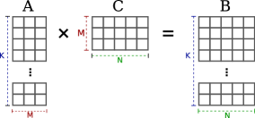
\subsection{Data␣from␣$\CM$}
\begin{figure}
␣␣\centering
␣␣\includegraphics[scale=0.5]{tsmm_mapping_u.pdf}
␣␣\caption{\emph{TSMM}:␣Parallelization␣over␣$K$␣and␣$N$␣and␣$2\times$
␣␣␣␣unrolling,␣two␣threads␣compute␣two␣results␣each␣and␣on␣two␣rows␣of
␣␣␣␣$\BM$␣in␣a␣single␣iteration.␣Slice␣horizontal␣to␣the␣$M$␣axis,␣the
␣␣␣␣$K$␣axis␣extends␣“indefinitely’’␣on␣both
␣␣␣␣sides.}␣\label{fig:tsmm_mapping_u}
\end{figure}
Our␣discussion␣of␣thread␣mappings␣and␣data␣transfers
so␣far␣has␣ignored␣the␣entries␣of␣the␣matrix␣$\CM$.␣These␣values␣are␣the␣same␣for
every␣index␣of␣the␣$K$␣loop.
The␣fastest␣would␣be␣to␣load␣all␣entries␣of␣$\CM$␣into␣registers␣and
reuse␣them␣from␣there,␣but␣this␣strategy␣would␣quickly␣exceed
the␣number␣of␣available␣registers␣even␣at␣moderate␣$M$␣and␣$N$.
Since␣they␣are␣accessed
frequently␣and␣all␣threads␣in␣a␣thread␣block␣access␣similar␣values,
the␣contents␣of␣$\CM$␣should␣continuously␣stay␣in␣the␣L1␣cache,␣making
reloads␣of␣these␣values␣a␣question␣of␣L1␣cache␣bandwidth␣and␣not
memory␣latency.␣Each␣load␣from␣$\CM$␣loads␣between␣one␣to␣three␣128-\byte
cache␣lines,␣which␣would␣then␣be␣used␣for␣a␣single␣FMA.␣This
is␣higher␣than␣the␣sustainable␣ratio␣of␣one␣128-\byte␣cache␣line␣per
FMA.␣A␣solution␣is␣to␣reuse␣each␣value␣loaded␣from␣$\CM$
by␣unrolling␣the␣$K$␣loop␣and␣pulling␣the␣unrolled␣iterations␣inside
the␣$M$␣loop.␣Each␣iteration␣over␣$K$␣loads␣the␣same␣values␣of␣$\CM$,
which␣can␣subsequently␣be␣used␣for␣multiple␣iterations␣per␣load.
The␣loads␣from␣$\CM$␣can␣also␣be␣sped␣up␣by␣using␣the␣shared␣memory␣to
cache␣these␣loads.␣Threads␣in␣a␣thread␣block␣collaboratively␣load␣the
contents␣of␣$\CM$␣into␣the␣shared␣memory␣at␣the␣beginning␣of␣the
kernel.␣The␣loop␣over␣$K$␣is␣parallelized␣with␣a␣grid␣stride␣loop,
where␣only␣as␣many␣threads␣as␣necessary␣for␣full␣occupancy␣are
launched.␣Each␣kernel␣instantiation␣then␣computes␣on␣multiple␣rows␣of
$\BM$.␣Therefore,␣loading␣$\CM$␣into␣shared␣memory␣can␣be␣amortized
over␣many␣rows.
On␣the␣V100,␣the␣shared␣memory␣has␣the␣same␣bandwidth␣as␣the␣L1␣cache,
given␣that␣they␣occupy␣the␣same␣hardware␣structure.␣However,␣shared␣memory
accesses␣guarantee␣cache␣hits,␣as␣they␣avoid␣conflict␣misses␣with␣other␣data.
They␣also␣have␣a␣lower␣latency,␣since␣no␣tags␣have␣to␣be␣checked.
\section{Results:␣TSMTTSM}
\subsection{Transposition␣and␣Leap␣Frogging}
\begin{figure}
␣␣\centering
␣␣\includegraphics[scale=0.7]{tsmttsm_plot1.pdf}
␣␣\caption{Performance␣comparison␣of␣real-valued␣double-precision␣\emph{TSMTTSM}
␣␣␣␣vs.\␣quadratic␣tile␣size
␣␣␣␣with␣$K=2^{29}/M$␣on␣the␣V100␣across␣the␣four␣different␣permutations␣of␣using␣leap
␣␣␣␣frogging␣(LF)␣and␣transposed␣mapping␣(trans).␣The␣best␣performance␣for
␣␣␣␣each␣matrix␣size␣and␣configuration␣is␣shown.␣The␣arithmetic␣peak␣performance
␣␣of␣the␣device␣is␣$7.066\,\TFS$.}␣\label{fig:perfperm}
\end{figure}
An␣exhaustive␣search␣was␣used␣to␣find␣the␣best␣tile␣size␣and
configuration␣for␣each␣matrix␣size.␣The␣simpler␣mapping␣schemes␣are␣subsets
of␣the␣tiled␣mapping.␣E.g.,␣the␣mapping␣in␣Figure~\ref{fig:genv3}␣corresponds
to␣a␣tilesize␣of␣$M\times␣1$.␣Figure~\ref{fig:perfperm}␣shows
the␣performance␣of␣the␣four␣configurations␣of␣using␣leap␣frogging␣and
a␣transposed␣mapping.␣␣The␣performance␣agrees␣with␣the␣roof\/line␣prediction
(dashed␣line)␣perfectly␣until␣$M,N=20$.␣Until␣$M,N=36$,␣the␣best
performance␣stays␣within␣95\%␣of␣the␣limit.␣␣Beyond␣that,␣the␣growing
arithmetic␣intensity␣does␣not␣translate␣into␣a␣proportional␣speedup
anymore,␣although␣the␣performance␣is␣still␣about␣a␣factor␣of␣two␣away
from␣peak.␣The␣best␣variants␣plateau␣at␣about
4700\,\GFS,␣or␣\sfrac{2}{3}␣of␣peak.␣␣Both␣variants␣using␣leap
frogging␣are␣clearly␣faster,␣but␣the␣transposed␣mapping␣is␣only
a␣bit␣faster␣if␣leap␣frogging␣is␣used.␣This␣is␣in␣contrast␣to␣experiences
with␣the␣\emph{Kepler}␣GPU␣architecture,␣where␣strided␣loads␣are␣slower,␣and␣this␣kind
of␣transformation␣is␣more␣beneficial.␣The␣best␣tile␣size␣changes␣when
leap␣frogging␣is␣used␣as␣it␣requires␣more␣registers.
\subsection{Tile␣Sizes}
\begin{figure}
\centering
\includegraphics[scale=0.7]{perf_vs_tilesize32x32trans.pdf}
\caption{Performance␣of␣\emph{TSMTTSM}␣for␣$M,N=32$␣and␣$K=2^{29}/M$
␣␣vs.\␣tile␣sizes␣in␣$M$␣and␣$N$␣directions,
␣␣using␣real-valued␣double-precision␣matrices,␣with␣leap␣frogging␣and
␣␣transposed␣mapping.␣The␣two␣white␣lines␣are␣defined␣by
␣␣$2␣\times␣(T_MT_N␣+␣2(T_M+T_N)␣+␣8)␣=␣R$,␣with␣$R=128,␣256$
␣␣to␣mark␣approximate
␣␣boundaries␣of␣register␣usage.}␣\label{fig:tileperf}
\end{figure}
Figure~\ref{fig:tileperf}␣shows␣the␣dependence␣of␣performance␣on␣the␣tile
sizes␣$T_M$␣and␣$T_N$␣for␣the␣case␣$M,N=32$␣with␣leap␣frogging␣and
transposed␣mapping.␣Performance␣drops␣off␣sharply␣if␣the␣tile␣sizes
become␣too␣large␣and␣too␣many␣registers␣are␣used.␣The␣number␣of
registers␣can␣be␣approximated␣by␣$2␣\times␣(T_MT_N␣+␣2(T_M+T_N)␣+␣8)$,
which␣accounts␣for␣the␣thread-local␣sums␣($T_MT_N$),␣loaded␣values
$(T_M+T_N)$,␣and␣eight␣registers␣for␣other␣purposes.␣Leap␣frogging
introduces␣a␣factor␣of␣two␣for␣the␣number␣of␣loaded␣values␣(for
\emph{current}␣and␣\emph{next}␣values),␣and␣double␣precision␣values␣generally
require␣two␣32-\bit␣registers␣for␣an␣overall␣factor␣of␣two.␣The␣graph␣shows␣the
iso-lines␣of␣128␣and␣256␣registers,␣which␣represent␣the␣occupancy␣drop
from␣25\%␣to␣12.5\%␣at␣128␣registers␣and␣the␣onset␣of␣spilling␣at␣256
registers.
The␣best-performing␣tile␣sizes␣generally␣sit␣on␣or␣just␣below␣these
lines,␣maximizing␣the␣area␣of␣the␣tile␣for␣a␣given␣occupancy.␣The
dimensions␣are␣largely␣symmetric␣but␣not␣perfectly␣so,␣as␣threads␣are
mapped␣to␣tiles␣in␣$M$␣direction␣first.␣There␣are␣clear␣patterns
favoring␣powers␣of␣two␣as␣those␣are␣divisors␣of␣the␣matrix␣size␣32
and␣avoid␣both␣the␣overhead␣of␣guarding␣statements␣and␣idle␣threads.
\subsection{Analysis}
According␣to␣the␣roof\/line␣model,␣at␣$M=N=64$
the␣upper␣performance␣limit␣is
\bq
P=\frac{64}{8}\frac{\flop}{\byte}␣\times␣880\,\GBS␣=␣7060\,\GFS\cma
\eq
which␣is␣almost␣exactly␣the␣$P_{Peak}$␣of␣$7066\,\GFS$.
However,␣our␣implementation␣cannot␣realize␣the␣roof\/line-predicted
performance,␣and␣instead␣tops␣out␣at␣$4766\,\GFS\approx\sfrac{2}{3}P_{Peak}$.
The␣reason␣for␣the␣limitation␣is␣memory␣latency,
%the
%third␣large␣performance␣limiter␣next␣to␣instruction␣throughput␣and
%memory␣bandwidth.
which␣can␣be␣shown␣by␣a␣simple␣model:
Whereas␣the␣memory␣latency␣for␣an␣idle␣memory␣interface␣measured␣with
a␣pointer␣chasing␣benchmark␣(see~\cite{cuda-benches})␣is␣only
435\,\cycles,␣this␣latency␣increases␣as␣the␣load␣on␣the␣memory␣interface
increases.␣For␣the␣values␣in␣Table~\ref{tab:membw},␣it␣is␣possible␣to
calculate␣corresponding␣latency␣values␣according␣to␣Little’s Law via
\bq\label{eq:little}
T_\ell=\frac{fN \times 8\,\byte}{b}\cma
\eq
with $f$ being the clock frequency, $N$
the thread count and $b$ the memory bandwidth. For the unloaded case in the
first row of Table~\ref{tab:membw} (ILP=1), the latency
according to (\ref{eq:little}) is $T_\ell\approx 470\,\cycles$,
%\GHZ\:\cdot\:128\:\cdot\: 8\mathrm{Byte} / 3 \GBS = 470 \cycle$,
which matches the measured pointer chasing latency quite well.
The bandwidth of $b=681\,\GBS$ at 25\% occupancy
in the fourth row roughly corresponds to the highest observed memory
bandwidth, based on the computational intensity,
for $M,N=64$, and result in $T_\ell\approx 664\,\cycles$
%$1.38 \GHZ\:\cdot\:80 \cdot
%512\:\cdot\: 8\mathrm{Byte} / 681 \GBS = 664 \cycle$
of memory latency.
The best tile size without leap frogging is $11\times8$, which
requires $11 \times 8 = 88$~FMA operations. These can be computed on a
single quadrant in $88\times 4\,\cycles=352\,\cycles$. At this large tile
size, the register requirements of at least $2\times11\times8=176$
registers allow to run only eight warps, i.e., two warps per quadrant,
simultaneously on a SM. One warp doing 352\,\cycles of compute
work finishes earlier than the other warp waiting for 664\,\cycles for
data from memory. It will then also wait for the next data to be
loaded, which is a period of time where none of the two warps are
issuing floating point operations, and therefore counts as wasted cycles.
Leap frogging does improve the situation, as even with a single warp
the memory latency and compute times can overlap. However, additional
registers are required to hold the data for the next iteration, which
either necessitates smaller tile sizes or reduces occupancy, both of
which are bad for overlapping. Overall, leap frogging is still beneficial,
though.
\begin{figure}
\centering
\includegraphics[scale=0.7]{perf_vs_occupancy.pdf}
\caption{\emph{TSMTTSM} performance vs.\ occupancy of real, correct kernels and two
modified (incorrect) kernels at tile sizes of $4\times 8$ and $8\times 8$,
respectively. The first modification reduces
register count, while the second kernel additionally reduces the data
set so that it resides in L1 cache. Green circles mark the point
with the highest performance of the unmodified kernels. (Real-valued
double-precision matrices)} \label{fig:perfoccupancy}
\end{figure}
Figure~\ref{fig:perfoccupancy} shows an experiment that gives insight
into the relationship of latency and occupancy. A modification of the
generated kernels allows testing the impact of higher occupancies even
for kernels with larger tile sizes, where the high register
requirements usually limit the occupancy to the minimum of eight
warps per SM. Instead of computing $T_M\times T_N$ intermediate results, all
summands are summed up in just two accumulators. This does of course
not compute the correct results any more, but all the instructions and
loaded operands are the same, while reducing the register count so
that 32 warps per SM can run concurrently. Another modification to the
generated kernel introduces a division of the $K$ loop row index by a
large constant. In consequence, all loop iterations compute on data of
very few rows, which makes almost all accesses L1 cache hits with the
corresponding much smaller latency. Repeatedly using the same row is
done in such a contrived way in order to prevent the compiler from
pulling the loads in front of the loop.
With tile sizes of $8\times 4$ and $8 \times 8$, as used in this
experiment, 16 and 8 warps per SM can run concurrently. At these
occupancies (green circles in Figure~\ref{fig:perfoccupancy}),
the respective real kernels (circle symbols) performance is highest,
as the maximum possible number of
thread blocks run concurrently. With an increased number of launched
thread blocks, the unmodified kernels’␣performance␣does␣not␣increase
anymore,␣as␣additional␣thread␣blocks␣do␣not␣run␣concurrently␣but␣are
scheduled␣in␣a␣“second␣wave’’␣of␣thread␣blocks.␣An␣imbalance␣in␣the
number␣of␣thread␣blocks␣per␣wave␣leads␣to␣fluctuating␣performance.
The␣kernels␣modified␣for␣higher␣occupancy␣(triangle␣symbols)␣have
the␣same␣performance␣as␣the␣unmodified␣kernels␣up␣to␣these␣points,␣but
allow␣to␣see␣the␣hypothetical␣speedup␣if␣more␣thread␣blocks
could␣run␣concurrently,␣which␣would␣be␣possible␣on␣a␣hypothetical
V100␣with␣$4\times$␣larger␣register␣files.
The␣performance␣increase␣is␣linear␣in␣all␣cases␣up␣to␣four␣warps␣per␣SM,␣as␣this␣is
the␣minimum␣to␣fill␣all␣four␣quadrants␣of␣a␣SM.␣For␣both␣tile␣sizes,
the␣L1␣load␣kernels␣(square␣symbols)␣profit␣somewhat␣from␣a␣second
warp␣on␣each␣quadrant␣to␣overlap␣the␣remaining␣latency␣and␣overhead
but␣quickly␣saturate␣at␣ceilings␣of␣$6080\,\GFS$␣and␣$5700\,\GFS$,
respectively,␣which␣is␣not␣a␣latency␣effect␣any␣more.␣The␣reason␣for␣these
lower␣roofs␣remains␣open,␣but␣we␣suspect␣that␣it␣be␣rooted␣in␣limited
instruction␣throughput.
We␣noticed␣that␣the␣gap␣to␣the␣device␣peak␣performance
matches␣one␣missing␣DP␣FP␣operation␣per␣four␣non-DP␣FP␣operations,
i.e.,␣integer␣and␣load␣instructions.␣DP␣FP␣operations␣are␣supposed␣to
execute␣on␣separate␣execution␣units,␣and␣so␣we␣can␣only␣speculate
whether␣there␣is␣a␣restriction␣in␣co-issuing␣DP␣FP␣operations␣with
integer␣and␣load␣instructions.
The␣two␣experiments␣with␣the␣normal,␣higher␣latency␣from␣memory␣(triangular
symbols)␣need␣many␣more␣warps␣to␣overlap␣their␣longer␣latency␣to
eventually␣saturate␣at␣the␣same␣level␣as␣the␣L1␣load␣kernels.␣At␣least
two␣to␣three␣times␣larger␣register␣files␣would␣be␣required␣to␣get
there.␣␣At␣the␣same␣time,␣it␣also␣shows␣how␣devastating␣it␣would␣be␣if
the␣register␣files␣were␣half␣as␣large,␣a␣situation␣that␣is␣not␣dissimilar␣to
the␣older␣\emph{Kepler}␣GPU␣architecture,␣where␣double␣the␣number␣of␣execution␣units
were␣backed␣by␣a␣similar␣sized␣register␣file.
The␣larger␣tile␣size␣saturates␣more␣quickly,
because␣it␣amortizes␣the␣same␣latency␣over␣twice␣the␣number␣of
floating-point␣operations.␣Note␣that␣in␣the␣end,␣both␣tile␣sizes␣have
a␣similar␣real␣world␣performance,␣as␣the␣higher␣possible␣occupancy␣of
16␣warps␣per␣SM␣compared␣to␣8␣warps␣per␣SM␣balances␣the␣smaller␣amount␣of␣work
per␣iteration.
This␣simple␣model␣also␣helps␣to␣explain␣the␣rather
small␣benefits␣from␣using␣the␣transposed␣mapping.␣The␣transposed␣mapping
changes␣the␣load␣pattern␣to␣contiguous␣blocks␣instead␣of␣long
strides.␣This␣in␣turn␣reduces␣the␣number␣of␣touched␣cache␣lines,␣and
increases␣the␣rate␣at␣which␣the␣L1␣cache␣can␣serve␣the␣outstanding␣loads
after␣the␣data␣has␣arrived␣from␣memory.␣However,␣this␣rate␣is␣only
really␣a␣limiter␣at␣low␣FMA/load␣ratios,␣or␣at␣the␣beginning␣of␣the
floating-point␣operation␣phase,␣where␣the␣FP␣units␣still
wait␣for␣enough␣registers␣being␣filled␣for␣uninterrupted␣operation.␣The
transposed␣mapping␣therefore␣only␣gives␣a␣small␣speedup␣in␣phase
that␣is␣mostly␣not␣the␣limiter,␣but␣at␣the␣same␣time␣also␣makes
smaller␣tile␣sizes␣more␣feasible.
On␣the␣other␣hand,␣the␣strided␣access␣patterns␣of␣the␣nontransposed␣mapping
touch␣most␣cache␣lines␣already␣on␣the␣first␣load,␣and␣therefore␣already
cause␣most␣cache␣misses␣with␣the␣first␣load.␣Subsequent␣loads␣are␣cache␣hits.
With␣the␣transposed␣mapping,␣with␣its␣contiguous␣blocks␣of␣addresses␣per␣load,
cache␣misses␣are␣postponed␣until␣later␣loads,␣which␣starts␣the␣memory␣latency
penalty␣later.␣That␣is␣why␣the␣configuration
using␣the␣transposed␣mapping␣without␣leap␣frogging␣performs␣the␣worst␣(see
Figure~\ref{fig:perfperm}).␣However,
in␣combination␣with␣leap␣frogging␣it␣is␣faster␣than␣the␣two␣variants␣with␣the
nontransposed␣mapping.
\subsection{Comparison␣with␣Libraries}
\begin{figure}
␣␣\centering
␣␣\includegraphics[scale=0.7]{tsmttsm_plot2.pdf}
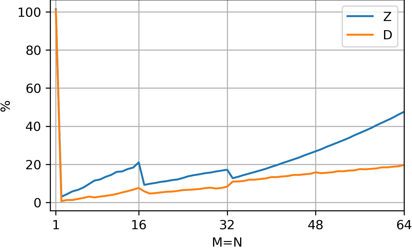
␣␣\caption{\emph{TSMTTSM}␣percentage␣of␣roof\/line-predicted␣performance␣for␣real␣(D)␣and
␣␣␣␣complex␣(Z)␣double-precision␣data␣in␣comparison␣with␣CUBLAS␣and
␣␣␣␣CUTLASS.}␣\label{fig:bestflop}
\end{figure}
Both␣CUBLAS’ and CUTLASS’␣performance␣is␣far␣below␣the␣potential
performance,␣except␣for␣$M,N=1$,␣where␣CUBLAS␣seems␣to␣have␣a␣special
detection␣for␣the␣scalar␣product␣corner␣case.␣The␣utilization␣of
potential␣performance␣increases␣as␣matrices␣become␣wider,␣which␣makes
them␣more␣square␣and␣compute␣bound,␣bringing␣them␣closer␣to␣more
standard␣scenarios.
In␣contrast,␣the␣presented␣implementation␣shows␣full␣efficiency␣for
narrow,␣clearly␣memory␣bandwidth␣limited␣matrices,␣and␣utilization
slightly␣drops␣off␣as␣matrices␣become␣more␣compute␣bound.␣For
complex-valued␣matrices,␣the␣\emph{TSMTTSM}␣becomes␣compute␣bound
already␣at␣$M,N=32$.␣Instruction␣throughput␣becomes␣the␣limiter␣much
earlier␣instead␣of␣memory␣bandwidth␣and␣latency,␣which␣is␣why␣the
utilization␣drops␣earlier.␣With␣increasing␣matrix␣size,␣it␣fully
saturates␣the␣previously␣explained␣lower␣ceiling␣due␣to␣our␣speculated
co-issue␣limitation␣between␣double-precision␣FP␣instructions␣and
integer␣instructions.
\subsection{Impact␣of␣Reductions}\label{sec:reductions}
\begin{figure}
␣␣\centering
␣␣\includegraphics[scale=0.6]{reduction_perf.pdf}
␣␣\caption{Global␣reduction␣impact␣for␣\emph{TSMTTSM}:
␣␣␣␣Performance␣when␣using␣each
␣␣␣␣of␣the␣two␣global␣reduction␣variants␣as␣the␣percentage␣of␣the
␣␣␣␣performance␣of␣a␣kernel␣without␣a␣global␣reduction,␣using␣two␣different
␣␣␣␣matrix␣widths␣and␣tile␣sizes.␣(Real-valued␣double-precision
␣␣␣␣matrices).}\label{fig:red_perf}
\end{figure}
Figure~\ref{fig:red_perf}␣shows␣the␣relative␣performance␣of␣our␣\emph{TSMTTSM}
implementation␣versus␣row␣count␣with␣respect␣to␣a␣baseline␣without␣any
reduction␣for␣a␣selection␣of␣inner␣matrix␣sizes␣and␣tile␣sizes,
choosing␣either␣of␣the␣two␣reduction␣methods␣described␣in
Section~\ref{sec:globred}.␣␣As␣expected,␣the␣impact␣of␣the␣reduction
generally␣decreases␣with␣increasing␣row␣count.␣The␣method␣with␣only
global␣atomics␣is␣especially␣slow␣for␣the␣narrower␣matrices
($M,N=4$).␣Many␣threads␣writing␣to␣a␣small␣amount␣of␣result␣values
leads␣to␣contention␣and␣causes␣a␣noticeable␣impact␣even␣for␣a␣matrix
filling␣the␣device␣memory␣($K=10^8$).␣The␣local␣atomic␣variant␣drastically
reduces␣the␣number␣of␣writing␣threads,␣resulting␣in␣less␣than␣10\%
overhead␣even␣for␣the␣smallest␣sizes␣and␣near-perfect␣performance␣for␣$K>10^6$.
For␣the␣wider␣matrices,␣the␣difference␣is␣smaller.␣The␣global␣atomic
version␣is␣not␣as␣slow␣because␣writes␣spread␣out␣over␣more␣result
values␣and␣the␣local␣atomic␣variant␣is␣not␣as␣fast␣because␣the␣larger␣tile␣size
requires␣more␣work␣in␣the␣local␣reduction.␣Both␣variants␣incur␣less␣than␣$10\%$
overhead␣just␣above␣$K=10^4$,␣a␣point␣where␣only␣about␣$0.2\%$␣of␣the␣GPU
memory␣is␣used.
\section{Results:␣TSMM}
The␣described␣methods␣and␣parameters␣open␣up␣a␣large␣space␣of␣configurations.
Each␣of␣the␣Figures~\ref{fig:tsmmplot1},␣\ref{fig:tsmmplot2},␣and␣\ref{fig:tsmmplot3}
shows␣a␣cross␣section␣of␣each␣configuration␣option␣by␣displaying␣the␣best-performing
value␣for␣each␣choice␣for␣that␣configuration␣option.
\subsection{Source␣of␣$\CM$}
\begin{figure}
␣␣\centering
␣␣\includegraphics[scale=0.7]{tsmm_plot1.pdf}
␣␣\caption{\emph{TSMM}␣performance␣comparison␣at␣$K=2^{29}/M$␣among
␣␣␣␣different␣sources␣for␣the␣matrix␣$\CM$,␣showing␣the
␣␣␣␣best-performing␣configuration␣of␣each␣method␣and␣matrix
␣␣␣␣width.␣(Real-valued␣double-precision␣matrices).}␣\label{fig:tsmmplot1}
\end{figure}
The␣data␣in␣Figure~\ref{fig:tsmmplot1}␣demonstrates␣that␣trying␣to␣keep␣the␣values␣of
matrix␣$\CM$␣in␣registers␣works␣well␣only␣for␣small␣$M,N$.
The␣increasing␣register␣pressure␣at␣larger␣sizes␣reduces␣occupancy,␣which␣is
especially␣bad␣if␣multiple␣results␣are␣computed
per␣thread.
Reloading␣values␣from␣shared␣memory␣consistently␣has␣a␣small
performance␣advantage␣especially␣for␣sizes␣that␣are␣not␣multiples␣of
four,␣due␣to␣a␣smaller␣penalty␣because␣of␣misaligned␣loads.␣Each
additional␣cache␣line␣that␣gets␣touched␣because␣of␣misalignment␣costs
an␣additional␣cycle.
\subsection{Unrolling}
\begin{figure}
␣␣\centering
␣␣\includegraphics[scale=0.7]{tsmm_plot2.pdf}
␣␣\caption{\emph{TSMM}␣performance␣comparison␣of␣different␣degrees␣of
␣␣␣␣unrolling␣at␣$K=2^{29}/M$,␣showing␣the␣best-performing␣configuration
␣␣␣␣for␣each␣unrolling␣depth␣($1,\ldots,4$)
␣␣␣␣and␣matrix␣width.␣(Real-valued␣double-precision
␣␣␣␣matrices).}␣\label{fig:tsmmplot2}
\end{figure}
Although␣there␣is␣little␣improvement␣with␣further␣unrolling␣beyond
$2\times$,␣as␣Figure~\ref{fig:tsmmplot2}␣shows,␣unrolling␣at␣least
once␣shows␣a␣clear␣speedup␣compared␣to␣no␣unrolling.␣Without
unrolling,␣the␣shared␣memory␣bandwidth␣would␣limit␣the␣performance
due␣to␣the␣high
ratio␣of␣shared␣memory␣loads␣to␣FP␣DP␣instructions,␣and␣its␣latency
could␣not␣be␣hidden␣as␣well␣with␣FP␣DP␣instructions␣from␣further
iterations.␣␣Generally,␣a␣similar␣reasoning␣as␣for␣the␣\emph{TSMTTSM}
kernel␣applies,␣where␣computing␣more␣results␣per␣thread␣and␣higher
unrolling␣counts␣increase␣the␣number␣of␣floating-point␣operations␣per
iteration␣but␣also␣decrease␣the␣occupancy␣that␣would␣be␣needed␣to
overlap␣the␣memory␣latency.
\subsection{Thread␣Count}
\begin{figure}
␣␣\centering
␣␣\includegraphics[scale=0.7]{tsmm_plot3.pdf}
␣␣\caption{\emph{TSMM}␣performance␣comparison␣of␣different␣thread
␣␣␣␣counts␣per␣row␣at␣$K=2^{29}/M$,␣showing␣the␣best-performing␣configuration␣for
␣␣␣␣each␣thread␣count␣and␣matrix␣width.␣(Real-valued␣double-precision␣matrices).}
␣␣\label{fig:tsmmplot3}
\end{figure}
Fewer␣threads␣per␣row␣mean␣more␣work␣per␣thread.␣For␣large
matrix␣sizes,␣this␣can␣result␣in␣huge␣kernels␣with␣high␣register
requirements,␣which␣is␣why␣Figure~\ref{fig:tsmmplot3}␣does␣not␣show
measurements␣for␣the␣whole␣matrix␣size␣range␣for␣one␣and␣two␣threads
per␣row.␣These␣two␣thread␣counts␣are␣the␣slowest␣variants,␣as␣they
show␣the␣effects␣of␣strided␣writes␣the␣most.␣With␣four␣threads␣writing
consecutive␣values,␣there␣is␣at␣least␣a␣chance␣of␣writing␣a␣complete
32-\byte␣cache␣line␣sector.␣The␣difference␣between␣4,␣8␣or␣16␣threads␣is
not␣large,␣although␣the␣larger␣thread␣counts␣perform␣slightly␣more
consistently␣(i.e.,␣with␣less␣fluctuation␣across␣$M$).
The␣performance␣analysis␣for␣\emph{TSMM}␣shows␣a␣clear
preference␣for␣the␣small␣matrix␣dimension␣$M=N$␣to␣be␣a␣multiple␣of
four.␣For␣this␣case,␣all␣writes␣of␣computed␣data␣to␣the␣matrix␣$\BM$␣are
aligned␣to␣$4␣\times␣8␣\,\byte␣=␣32␣\,\byte$,␣which␣is␣the␣management
granularity␣for␣L1␣cache␣lines␣and␣the␣cache␣line␣length␣for␣the␣L2
cache.␣With␣this␣alignment,␣cache␣lines␣are␣fully␣written␣and␣there␣is
no␣overhead␣for␣write␣allocation␣from␣memory.␣Misalignment␣is␣the
major␣performance␣hurdle␣for␣matrix␣widths␣that␣are␣not␣multiples␣of
four.
\subsection{Comparison␣with␣Libraries}
\begin{figure}
␣␣\centering
␣␣\includegraphics[scale=0.7]{tsmm_plot4.pdf}
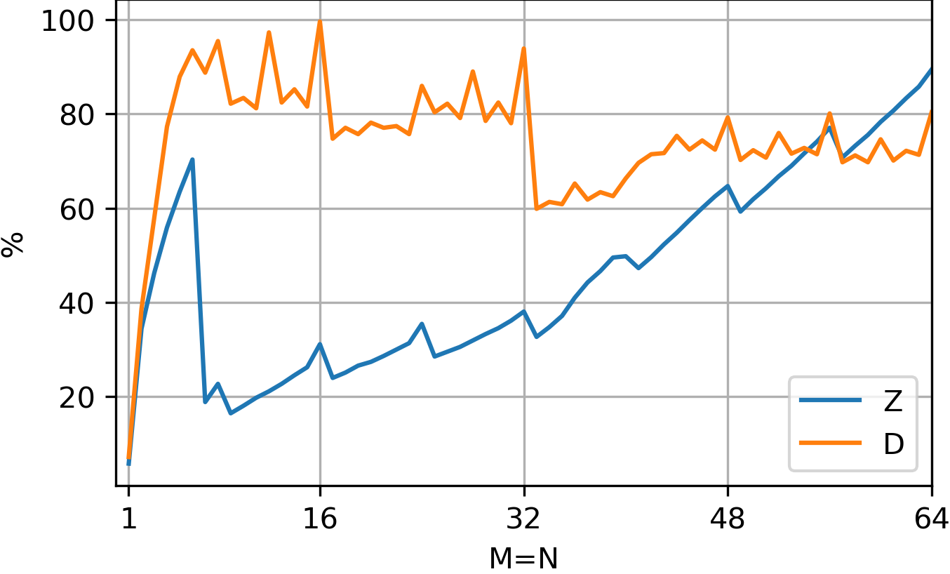
␣␣\caption{\emph{TSMM}␣percentage␣of␣roof\/line-predicted␣performance␣for␣real
␣␣␣␣(D)␣and␣complex␣(Z)␣double-precision␣data␣in␣comparison␣with␣CUBLAS.}
␣␣\label{fig:tsmmplot4}
\end{figure}
Figure~\ref{fig:tsmmplot4}␣shows␣that,␣except␣for␣very␣small␣$M,N$,
CUBLAS␣performs␣very␣well␣for␣the␣real-valued␣\emph{TSMM}
kernel.␣With␣increasing␣width,␣the␣development␣in␣utilization␣is
very␣similar␣to␣the␣presented␣implementation.␣Our␣solution
works␣similarly␣well␣for␣complex␣values␣matrices,␣which␣is␣not␣the
case␣for␣CUBLAS.␣Here,␣a␣strong␣performance␣drop␣for␣medium-wide␣matrices
can␣be␣observed.
\section{Conclusion␣and␣Outlook}
We␣have␣shown␣how␣optimize␣the␣performance␣for␣two
types␣of␣multiplication␣of␣double-precision,␣real␣and␣complex␣tall␣\&
skinny␣matrices␣on␣a␣V100␣GPU.␣With␣matrices
narrower␣than␣32␣columns,␣perfect␣performance␣in␣accordance
with␣a␣roof\/line␣performance␣model␣could␣be␣achieved.
Over␣the␣rest␣of␣the␣skinny␣range␣up␣to␣a␣width␣of␣64,
between␣60\%␣and␣\sfrac{2}{3}␣of␣the␣potential␣performance␣was
attained.
We␣used␣a␣code␣generator␣on␣top␣of␣a␣range␣of
suitable␣thread␣mapping␣and␣tiling␣patterns,␣which␣enabled␣an
exhaustive␣parameter␣space␣search.␣␣Two␣different␣ways␣to␣achieve
fast,␣parallel␣device-wide␣reductions␣for␣long␣vectors␣have␣been
devised␣in␣order␣to␣ensure␣a␣fast␣ramp-up␣of␣performance␣already␣for
shorter␣matrices.
%The␣roof\/line␣model␣was␣used␣consistently␣as␣a
%performance␣yardstick.
An␣in-depth␣performance␣analysis␣was␣provided
to␣explain␣observed␣deviations␣from␣the␣roof\/line␣limit.
Our␣implementation␣outperforms␣the␣vendor-supplied␣CUBLAS␣and␣CUTLASS
libraries␣by␣far␣or␣is␣on␣par␣with␣them␣for␣most␣of␣the␣observed
parameter␣range.
In␣future␣work,␣in␣order␣to␣push␣the␣limits␣of␣the␣current␣implementation,
shared␣memory␣could␣be␣integrated␣into␣the␣mapping␣scheme␣to␣speed␣up␣the␣many
loads,␣especially␣scattered␣ones,␣that␣are␣served␣by␣the␣L1␣cache.
The␣presented␣performance␣figures␣were␣obtained␣by␣parameter␣search.
An␣advanced␣performance␣model,␣currently␣under␣development,␣could␣be␣fed␣with
code␣characteristics␣such␣as␣load␣addresses␣and␣instruction␣counts␣generated
with␣the␣actual␣code␣and␣then␣used␣to␣eliminate␣bad␣candidates␣much␣faster.
It␣will␣also␣support␣a␣better␣understanding␣of␣performance␣limiters.
Prior␣work␣by␣us␣in␣this␣area␣is␣already␣part␣of␣the␣sparse␣matrix␣toolkit
\emph{GHOST}␣(\cite{GHOST})␣and␣we␣plan␣to␣integrate␣the␣presented␣work
there␣as␣well.\medskip
\begin{funding}
This␣work␣was␣supported␣by␣the␣ESSEX-II␣project␣in␣the␣DFG␣Priority␣Programme␣SPPEXA.
\end{funding}
\bibliographystyle{SageH}
\bibliography{references}
\end{document}
%%%␣Local␣Variables:
%%%␣mode:␣latex
%%%␣TeX-master:␣t
%%%␣End:’