QMUL-PH-19-12

Nikhef/2019-015

MS-TP-19-08

Diagrammatic resummation of leading-logarithmic threshold effects at next-to-leading power

N. Bahjat-Abbas^a, D. Bonocore^b, J. Sinninghe Damsté^c,d, E. Laenen^c,d,e,
L. Magnea^f, L. Vernazza^d and C. D. White^a

^a Centre for Research in String Theory, School of Physics and Astronomy, Queen Mary University of London, 327 Mile End Road, London E1 4NS, UK

^b Institut für Theoretische Physik, Westfälische Wilhelms-Universität Münster, Wilhelm-Klemm-Straße 9, D-48149 Münster, Germany

^c ITFA, University of Amsterdam, Science Park 904, Amsterdam, The Netherlands

^d Nikhef, Science Park 105, NL-1098 XG Amsterdam, The Netherlands

^e ITF, Utrecht University, Leuvenlaan 4, Utrecht, The Netherlands

^f Dipartimento di Fisica Teorica and Arnold-Regge Center, Università di Torino, and

INFN, Sezione di Torino, Via Pietro Giuria 1, I-10125 Torino, Italy

Perturbative cross-sections in QCD are beset by logarithms of kinematic invariants, whose arguments vanish when heavy particles are produced near threshold. Contributions of this type often need to be summed to all orders in the coupling, in order to improve the behaviour of the perturbative expansion, and it has long been known how to do this at leading power in the threshold variable, using a variety of approaches. Recently, the problem of extending this resummation to logarithms suppressed by a single power of the threshold variable has received considerable attention. In this paper, we show that such next-to-leading power (NLP) contributions can indeed be resummed, to leading logarithmic (LL) accuracy, for any QCD process with a colour-singlet final state, using a direct generalisation of the diagrammatic methods available at leading power. We compare our results with other approaches, and comment on the implications for further generalisations beyond leading-logarithmic accuracy.

1 Introduction

Perturbative calculations of hadronic cross sections in Quantum Chromodynamics (QCD) are the cornerstone of theoretical predictions for all processes of phenomenological interest at particle colliders, such as the Large Hadron Collider (LHC). Furthermore, the ever-increasing precision of experimental data demands that theoretical predictions for scattering processes of interest be continually improved. The relevant calculations are carried out using an expansion in powers of the coupling constant $\alpha_{s}$, and typically proceed on two fronts. First, one may determine the complete behaviour of a given quantity at a fixed order in the coupling constant. The state of the art for most processes is next-to-leading order (NLO) in perturbation theory, with an increasing number of notable exceptions known at NNLO, and even N³LO (see e.g. [1] for a review). Whilst successful for many observables, the fixed order approach is only valid provided subleading perturbative corrections are well-behaved. Given that perturbative coefficients depend on the momenta of the scattering particles, this criterion can fail in certain kinematic regimes: a well-known example is the production of heavy particles near threshold. In such processes, one can define a threshold variable $\xi$, which satisfies $\xi\rightarrow 0$ when the heavy particles carry all of the energy in the final state. The precise definition of $\xi$ will depend on the process being considered, but, generically, it has the form of a dimensionless ratio of kinematic invariants. One may then write a general schematic form for production cross-sections near threshold, as

$$\frac{d\sigma}{d\xi}\,=\,\sigma_{0}\sum_{n=0}^{\infty}\left(\frac{\alpha_{s}}{\pi}\right)^{n}\sum_{m=0}^{2n-1}\left[\,c_{nm}^{(-1)}\left(\frac{\log^{m}\xi}{\xi}\right)_{+}+\,c_{n}^{(\delta)}\,\delta(\xi)+\,c_{nm}^{(0)}\,\log^{m}\xi+{\cal O}(\xi)\,\right]\,.$$ (1)

Here we denote by $\sigma_{0}$ the Born-level cross section, which may contain additional coupling factors. The first contribution in the square brackets consists of a series of terms, at fixed order in $\alpha_{s}$, containing powers of the logarithm of the threshold variable, divided by $\xi$ itself. These contributions can be directly traced to soft and collinear singularities of the underlying scattering amplitudes: the cancellation of infrared divergences between virtual corrections and real radiation leaves behind potentially large corrections, which are still singular as $\xi\rightarrow 0$, but are regularised by the well-known plus prescription, so that they are integrable; as discussed below, the all-order structure of these terms is well understood. The second set of terms in Eq. (1) has support localised on the threshold, $\xi=0$, and for processes with electroweak final states it is known that such terms can be formally exponentiated (see, for example, Ref. [2]). The third set of terms in the square brackets is suppressed by a single power of $\xi$ with respect to the leading-power contribution. Although formally not as divergent as the preceding terms, they are nevertheless still singular as $\xi\rightarrow 0$, and thus potentially numerically sizeable in the threshold region. These next-to-leading power (NLP) terms are the focus of the present work, while we will neglect all further subleading contributions to Eq. (1), which vanish at threshold.

Order by order in perturbation theory, one can distinguish two expansions in Eq. (1). Firstly, there is an expansion in powers of the threshold variable $\xi$, in which we can distinguish the plus distributions and delta function terms as being leading power (LP) in $\xi$, while the remaining logarithms are next-to-leading-power (NLP). Secondly, for each fixed power of $\xi$, we can consider the expansion in powers of the logarithm, labelling terms proportional to $\log^{2n-1}\xi$ as leading logarithmic (LL), the next-highest power as next-to-leading logarithmic (NLL), and so on. The problematic nature of LP terms was noted already in the early days of QCD (see for example [3]), and it was quickly realised that such terms at LL level could be summed up to all orders in perturbation theory to achieve a well-behaved result as $\xi\rightarrow 0$ [4, 5]. This resummation was subsequently extended to subleading logarithmic accuracy using two equivalent approaches [6, 7, 8], themselves partially reliant on earlier diagrammatic arguments for the exponentiation of soft behaviour [9, 10, 11]. Since that time, LP threshold resummation has been reinterpreted and clarified using a wide variety of methods, including the use of Wilson lines [12, 13], the renormalisation group [14], the connection to factorisation theorems [15], and soft collinear effective theory (SCET) [16, 17, 18, 19]. The state of the art for resummation at LP is NNLL accuracy in many processes, including some cases of differential distributions. Recent, pedagogical reviews may be found in Refs. [20, 21, 22].

The phenomenological success of LP resummation, together with the increasing precision of contemporary collider data, makes it natural to ponder whether NLP terms in the threshold expansion can also be classified and resummed, particularly since they have been shown to be numerically significant in important scattering processes [23, 24]. Indeed, the study of such contributions has a long history. Subleading corrections involving soft momenta were first investigated in the classic works of Refs. [25, 26], which dealt exclusively with massive particles in QED. The analysis of Ref. [27] updated this to include massless particles. Some years later, the topic was investigated using path-integral methods in Ref. [28], which derived a set of effective Feynman rules for the emission of gauge bosons at next-to-soft level, and argued that a large class of NLP contributions exponentiates. The results were subsequently confirmed by an all-order analysis of Feynman diagrams [29], but concerned massive partons only. In a different approach, NLP effects in certain processes were argued to be resummable, based on well-motivated physical assumptions [30, 31, 32, 33, 34] (see also Refs. [35, 36, 37, 38, 39] for other work related to elucidating all-order properties).

More recently, there has been a revival of interest in studying NLP effects at amplitude level, partly motivated by more formal work relating soft radiation to asymptotic symmetries of the $S$-matrix in gauge theories and in gravity [40, 41]. Thus, in addition to the phenomenological applications mentioned above, the study of subleading threshold effects in quantum field theory can have a role to play in finding new representations of, and relations between, gauge and gravity theories [42, 43, 44, 45, 46, 47], whilst also finding applications in transplanckian scattering [48, 49, 50, 51]. In the latter context (as potentially in gauge theories), resummation plays a key role.

In QCD (and related gauge theories), threshold resummation at leading power is known to be a consequence of the universal factorisation of soft and collinear divergences in scattering amplitudes (see for example Ref. [15] for a dedicated discussion of this point). This has motivated attempts to construct a factorisation formula for NLP effects. References [52, 53] use a diagrammatic approach, building on the earlier work of Ref. [27], to describe the effect of dressing a general non-radiative amplitude with an additional gluon emission up to NLO, and NLP in the threshold expansion. This formula contains universal functions similar to those appearing at LP level, but including extra contributions that describe, for example, the emission of wide-angle soft gluons from within jets. A more complete analysis for scalar theories coupled to electromagnetism was undertaken in Refs. [54, 55, 56], which again stress the importance of new quantities (both universal and non-universal) that appear beyond LP order in emitted gluon momentum. Related analyses have been carried out in SCET [57, 58, 59, 60, 61, 62] (see Ref. [63] for earlier work in the context of flavour physics), and results using either diagrammatic or effective theory methods have been shown to be potentially useful for improving the accuracy of fixed-order calculations [64, 65, 66, 67, 68, 59, 69, 70, 71, 72, 73]. Recently, the SCET framework has been used to demonstrate that the leading-logarithmic (LL) NLP contributions can be resummed, first for event shapes [74], and then for Drell-Yan production [75], where the results agree with the predictions of the physical evolution kernel approach of Refs. [30, 31, 32, 33, 34].

Our aim in this paper is to show how a similar resummation of LL NLP effects can be achieved using the diagrammatic approach developed in Refs. [28, 29], and itself analogous to the original LP resummations of Refs. [6, 7, 9, 10, 11]. As in the SCET approach of Ref. [75] (and as observed in Refs. [52, 53, 54, 55, 56]), we will see that, while it is true that a number of new functions appear at NLP level in the threshold expansion, many of them are irrelevant for discussing the highest power of the NLP logarithm at any given order in perturbation theory. Thus, the resummation of LL NLP contributions is remarkably straightforward. Importantly, this method is sufficiently simple and universal that it can be directly applied to any hadronic cross section with colour-singlet final states: indeed, we explicitly discuss applications to Higgs boson production in the gluon fusion channel, and the formalism can readily be generalised to multi-boson final states. There are a number of motivations for the present analysis. First, they are a natural application of the programme of work commenced in refs. [28, 29], where it is was shown that a broad subclass of NLP effects indeed exponentiates. Second, the history of LP resummation suggests that it is highly useful to have more than one formalism for describing equivalent physics: comparison of one approach with another has the potential to clarify both, and it may also be the case that different approaches have relative strengths and weaknesses, thus being more or less suitable in any given context. Third, our diagrammatic approach will provide an alternative starting point for generalising the NLP resummation formalism beyond leading-logarithmic accuracy.

The structure of our paper is as follows. In Section 2, we review the resummation of LP threshold contributions, introducing notation that will be useful for what follows. In particular, we will relate our calculation to the path-integral methods of Ref. [28], which provide a particularly elegant proof of exponentiation. In Section 3, we show how the picture can be naturally extended to NLP level, using existing results. We will argue in detail that potential additional contributions to NLP behaviour, including hard collinear effects, non-universal behaviour and phase-space correlations between gluons, can be ignored at LL. Armed with this knowledge, we will then perform an explicit calculation that resums the LL NLP terms in Drell-Yan, comparing our results with others in the literature [30, 31, 32, 33, 34]. We will then comment on the general applicability of our framework to the production of an arbitrary number of colour singlet particles, before examining Higgs production in the large top mass limit as a further example. In Section 3.4, we briefly compare our framework with the recent analysis of Ref. [75], in the framework of Soft Collinear Effective Theory (SCET). Finally, we discuss our results in Section 4 before concluding. Technical details are collected in three appendices.

2 Threshold resummation at leading power

In this section, we review the resummation of terms at leading power in the threshold variable, using factorisation methods. Given that our aim in what follows is to sum leading-logarithmic terms only at NLP, we will mostly concern ourselves here with LL terms also at LP. Furthermore, we will phrase our discussion in terms of methods and notation that allow a straightforward generalisation to subleading power in the threshold expansion. While our discussion applies to general colour-singlet final states, we will first explicitly consider the Drell-Yan production of a massive (or off-shell) vector boson, which at LO corresponds to the partonic scattering process

$$q(p_{1})+\bar{q}(p_{2})\,\rightarrow\,V(Q)\,,$$ (2)

depicted in Figure 1. We will not explicitly consider here the quark-gluon production channel, where NLP logarithms are present, but constitute in fact the leading power, since LP logarithms are absent; in the gluon-gluon channel for the Drell-Yan process, only NNLP logarithms can arise.

Figure 1: Drell-Yan production at leading order.

We write the invariant mass distribution in the $q\bar{q}$ channel as

$$\frac{d\sigma}{d\tau}\,=\,\sigma_{0}(Q^{2})\int_{0}^{1}dzdx_{1}dx_{2}\,\delta(\tau-x_{1}x_{2}z)\,q(x_{1},\mu_{F}^{2})\,\bar{q}(x_{2},\mu_{F}^{2})\,\Delta\!\left(z,\alpha_{s}(\mu_{R}^{2}),\frac{\mu_{F}^{2}}{Q^{2}},\frac{\mu_{R}^{2}}{Q^{2}}\right)\,,$$ (3)

where we restrict ourselves to a single quark flavour for simplicity. Here $\sigma_{0}(Q^{2})$ is the total cross section, whose precise value will depend on the nature of the vector boson. Furthermore, $\alpha_{s}(\mu_{R}^{2})$ is the strong coupling at the renormalisation scale $\mu_{R}$, $q(x,\mu_{F}^{2})$ is a quark distribution function with longitudinal momentum fraction $x$ and factorisation scale $\mu_{F}$, while $\bar{q}$ is the equivalent for an antiquark. Given that scale choice effects contribute to only subleading logarithms (see for example [7]), we will simply choose $\mu_{F}=\mu_{R}=Q$ from now on, and simplify notation accordingly. In Eq. (3) we defined the invariants

$$\tau\,=\,\frac{Q^{2}}{s}\,,\qquad\qquad z\,=\,\frac{Q^{2}}{\hat{s}}\,,$$ (4)

where $\hat{s}=(p_{1}+p_{2})^{2}$ is the squared partonic centre of mass energy, and $s=\hat{s}/x_{1}x_{2}$ is the hadronic centre of mass energy. The ratio $z$ represents the fraction of $\hat{s}$ carried by the final state vector boson. At LO this must be unity, so that one has

$$\Delta^{(0)}\left(z\right)\,=\delta(1-z)\,.$$ (5)

The invariant mass distribution in Eq. (3) is a convolution in $z$, and can be diagonalised by taking Mellin moments with respect to $\tau$, with the result

$$\int_{0}^{1}d\tau\,\tau^{N-1}\,\frac{d\sigma}{d\tau}\,=\,\sigma_{0}(s,Q^{2})\,q(N,Q^{2})\,{\bar{q}}(N,Q^{2})\,\Delta(N,Q^{2})\,,$$ (6)

where

$$q(N,Q^{2})\,=\,\int dx\,x^{N-1}\,q(x,Q^{2})$$ (7)

is the transformed quark distribution (and similarly for the antiquark), and we have defined

$$\Delta(N,Q^{2})\,=\,\int_{0}^{1}dz\,z^{N-1}\,\Delta(z,Q^{2}).$$ (8)

Beyond LO, Eq. (8) receives potentially large threshold corrections. In Mellin space, these appear as contributions of the form

$$\alpha_{s}^{n}\,\log^{m}N\,,\qquad m\,=\,0,\ldots,2n\,,$$ (9)

which in momentum space are associated with plus distributions of the form

$${\cal D}_{i}\,=\,\left(\frac{\log^{i}(1-z)}{1-z}\right)_{+}\,,\qquad i\,=\,0,\ldots 2n-1\,,$$ (10)

defined such that

$$\int_{0}^{1}dz\,f(z)\,\big{[}g(z)\big{]}_{+}\,=\,\int_{0}^{1}dz\big{[}f(z)-f(1)\big{]}\,g(z)\,.$$ (11)

When computed in perturbation theory from quark scattering, $\Delta\left(N,Q^{2}\right)$ is affected by collinear divergences, which must be reabsorbed in the quark distributions: below, we will mostly work with the ‘bare’ $\Delta$, before renormalisation of the coupling $\alpha_{s}$, and before the factorisation of collinear divergences, which will be regulated using dimensional regularisation in $d=4-2\epsilon$. For clarity, we will denote this bare partonic cross section with $\widehat{\Delta}(z,Q^{2},\epsilon)$ in momentum space, and with $\widehat{\Delta}(N,Q^{2},\epsilon)$ in Mellin space. Collinear factorisation is understood to be performed in the $\overline{\rm MS}$ scheme.

For any QCD process with a colour-singlet final state produced near threshold, $\widehat{\Delta}$ has a factorised structure, and can be written as [6, 76]

$$\widehat{\Delta}\left(N,Q^{2},\epsilon\right)\,=\,\left|\mathcal{H}\left(Q^{2}\right)\right|^{2}\,\frac{\prod_{i}\psi_{i}\left(N,Q^{2},\epsilon\right)}{\prod_{i}\psi_{{\rm eik},i}\left(N,Q^{2},\epsilon\right)}\,{\cal S}\left(N,Q^{2},\epsilon\right)\,,$$ (12)

where $\mathcal{H}\left(Q^{2}\right)$ is an amplitude-level finite hard function containing off-shell virtual contributions, ${\cal S}(N,Q^{2},\epsilon)$ is a soft function collecting all soft enhancements associated with (real or virtual) soft radiation, and $\psi_{i}(N,Q^{2},\epsilon)$ is a perturbative (anti-)quark distribution function, collecting collinear singularities associated with initial line $i$; finally, given that infrared enhancements of both soft and collinear origin are included twice (both in the soft and quark distribution functions), one may remove the double counting by dividing each quark distribution by its own eikonal approximation $\psi_{{\rm eik},i}(N,Q^{2},\epsilon)$. Formal definitions of the (eikonal) quark distributions and of the soft function are given, for example, in Ref. [76]: sometimes, eikonal quark distributions are absorbed into the soft function to build the so-called reduced soft function, organising wide-angle soft radiation. On the other hand, one may consider the factor

$$\psi_{\,{\rm h},i}(N,Q^{2},\epsilon)\,=\,\frac{\psi_{i}(N,Q^{2},\epsilon)}{\psi_{{\rm eik},i}(N,Q^{2},\epsilon)}\,,$$ (13)

for each initial parton line: this has the effect of removing the soft behaviour from each quark distribution, leaving hard collinear behaviour only. This arrangement is particularly convenient if one wishes to focus only on leading logarithms, as we do in this paper: indeed, at any fixed order in $\alpha_{s}$, leading logarithms at leading power arise only when the maximum number of singular integrations is performed, yielding the highest inverse power of $\epsilon$. Thus, the factor $\psi_{{\rm h},i}(N,Q^{2},\epsilon)$ for each external line contributes only at subleading logarithmic accuracy, and can be put equal to unity at LL. We are then left with the simple result

$$\widehat{\Delta}\left(N,Q^{2},\epsilon\right)\,=\,\left|\mathcal{H}\left(Q^{2}\right)\right|^{2}{\cal S}\!\left(N,Q^{2},\epsilon\right)\,,$$ (14)

implying that leading logarithms in the DY cross-section at arbitrary orders in perturbation theory are governed purely by the soft function [6, 7, 13], on which we now focus.

For any QCD process with a colour-singlet final state, the soft function has a formal definition as a vacuum expectation value of Wilson line operators associated with the colliding partons. Defining the dimensionless four-vectors $\beta_{i}$ via

$$p_{i}^{\mu}\,=\,\sqrt{\hat{s}}\,\beta_{i}^{\mu}\,,$$ (15)

one may write the soft function (in momentum space) as

$${\cal S}(z,Q^{2},\epsilon)\,=\,\frac{1}{N_{c}}\sum_{n}\,{\rm Tr}\Big{[}\left\langle 0\left|\Phi_{\beta_{1}}^{\dagger}\Phi_{\beta_{2}}\right|n\right\rangle\left\langle n\left|\Phi_{\beta_{2}}^{\dagger}\Phi_{\beta_{1}}\right|0\right\rangle\Big{]}\,\delta\!\left(z-\frac{Q^{2}}{\hat{s}}\right)\,.$$ (16)

Here the trace is over colour indices, and the Wilson line operators are defined by

$$\Phi_{\beta_{i}}\,=\,{\cal P}\exp\left[{\rm i}g_{s}{\bf T}^{a}\int_{-\infty}^{0}d\lambda\,\beta_{i}\cdot A(\lambda\beta_{i})\right]\,,$$ (17)

where ${\bf T}^{a}$ is a colour generator in the fundamental representation; furthermore, Eq. (16) includes a sum over final states containing $n$ partons generated by the Wilson lines, including the appropriate phase space integration, and subject to the constraint that the total energy radiated in the final state equal $(1-z)\hat{s}$; finally, the division by the number of colours $N_{c}$ corrects for the fact that this factor has already been included in the LO cross-section $\sigma_{0}$ in Eq. (14). Introducing the momentum space gauge field $\tilde{A}_{\mu}(k)$, one may write the Wilson line exponent as

$${\rm i}g_{s}{\bf T}_{a}\int\frac{d^{d}k}{(2\pi)^{d}}\,\beta_{i}\cdot\tilde{A}(k)\int_{-\infty}^{0}d\lambda\,e^{{\rm i}\lambda\beta_{i}\cdot k}\,=\,\int\frac{d^{d}k}{(2\pi)^{d}}\,\tilde{A}_{\mu}(k)\left[g_{s}{\bf T}^{a}\,\frac{\beta_{i}^{\mu}}{\beta_{i}\cdot k-{\rm i}\varepsilon}\right]\,,$$ (18)

where the square-bracketed factor on the right constitutes the momentum-space factor associated to the emission of a gluon from the Wilson line. We recognise this as the well-known eikonal Feynman rule for soft gluon emission, so that finding the soft function amounts to calculating the cross section for the incoming partons in the eikonal approximation. This cross-section is known to exponentiate, which relies on two properties: first, vacuum expectation values of Wilson lines exponentiate before any phase space integrations are carried out, which may be shown diagrammatically [9, 10, 11], or using renormalisation group arguments, themselves relying on the multiplicative renormalisability of Wilson line operators [77, 78, 79, 80, 81, 82]; second, the phase space for the emission of $n$ soft partons factorises into $n$ decoupled one-parton phase space integrals, given that momentum conservation can be ignored at leading power in the threshold expansion.

Combining these two properties, one finds that the complete soft function, at cross-section level, has an exponential form, and the exponent can be directly computed in terms of a special class of Feynman diagrams known as webs [9, 10, 11]. These results have been reinterpreted more recently using a path integral approach [28], which incorporated statistical physics methods (the replica trick) to provide a particularly streamlined proof of diagrammatic exponentiation. These methods have in turn allowed the web language to be generalised to multiparton scattering [83, 84, 85, 86, 87, 88, 89, 90, 91] (see also [92, 93], or Ref. [94] for a pedagogical review). We review the replica trick here in Appendix A, given that it can also be used to demonstrate directly the exponentiation of a large class of contributions at NLP in the threshold expansion.

Concentrating on leading logarithms, it is important to note that the pattern of exponentiation of soft and collinear singularities is non-trivial, in that the exponent is single-logarithmic (containing terms of the form $\alpha_{s}^{n}\log^{m}N$ with $m\leq n+1$), while the cross section is double-logarithmic, as noted in Eq. (9). The leading logarithms for the cross sections are therefore completely determined by a one-loop evaluation, which we briefly review below. The eikonal cross-section, up to NLO and in momentum space, can be written as 

$${\cal S}\!\left(z,Q^{2},\epsilon\right)\,=\,\left(1+{\cal S}^{(1)}_{\rm virtual}\right)\delta(1-z)+{\cal S}^{(1)}_{\rm real}(z)+{\cal O}\left(\alpha_{s}^{2}\right)\,.$$ (19)

The real radiation contribution can be obtained from the graphs of Figure 2 using eikonal Feynman rules, and one finds

Figure 2: Real emission diagrams for the eikonal cross-section of Eq. (20), where all emission vertices are assumed to be eikonal.

$${\cal S}^{(1)}_{\rm real}(z)\,=\,\mu^{2\epsilon}g_{s}^{2}\,C_{F}\int\frac{d^{d}k}{(2\pi)^{d-1}}\,\delta_{+}(k^{2})\,\delta\!\left(1-z-\frac{2k\cdot(p_{1}+p_{2})}{\hat{s}}\right)\frac{2p_{1}\cdot p_{2}}{p_{1}\cdot k\,p_{2}\cdot k}\,.$$ (20)

The virtual contribution at ${\cal O}(\alpha_{s})$ can be obtained by direct calculation, or by imposing the soft gluon unitarity requirement

$$\int_{0}^{1}dz\,{\cal S}\!\left(z,Q^{2},\epsilon\right)\,=\,1\,,$$ (21)

reflecting the requirement that soft divergences from the virtual and real contributions must cancel, and the fact that Wilson line correlators are pure counterterms in dimensional regularisation. This requirement implies

$${\cal S}^{(1)}_{\rm virtual}\,=\,-\int_{0}^{1}dz\,{\cal S}^{(1)}_{\rm real}(z)\,,$$ (22)

so that the eikonal cross-section at ${\cal O}(\alpha_{s})$ can be written as

$${\cal S}^{(1)}(z)\,=\,\mu^{2\epsilon}g_{s}^{2}\,C_{F}\int\frac{d^{d}k}{(2\pi)^{d-1}}\,\bigg{[}\delta^{+}(k^{2})\,\delta\left(1-z-\frac{2k\cdot(p_{1}+p_{2})}{\hat{s}}\right)-\delta(1-z)\bigg{]}\frac{2p_{1}\cdot p_{2}}{p_{1}\cdot k\,p_{2}\cdot k}\,.$$ (23)

To carry out the momentum integral, it is particularly convenient to introduce the Sudakov decomposition

$$k^{\mu}\,=\,k_{+}\beta_{1}^{\mu}+k_{-}\beta_{2}^{\mu}+k_{T}^{\mu}\,,$$ (24)

where $k_{T}$ is a four-vector transverse to $\beta_{1}^{\mu}$ and $\beta_{2}^{\mu}$,

$$k_{T}\cdot\beta_{1}\,=\,k_{T}\cdot\beta_{2}\,=\,0\,.$$ (25)

Contracting Eq. (24) with $\beta_{1}^{\mu}$ and $\beta_{2}^{\mu}$, it is straightforward to verify that the components $k_{\pm}$ are given by

$$k_{+}\,=\,\frac{2p_{2}\cdot k}{\sqrt{\hat{s}}}\,,\qquad k_{-}\,=\,\frac{2p_{1}\cdot k}{\sqrt{\hat{s}}}\,;$$ (26)

furthermore, the integration measure in Eq. (23) becomes

$$\int d^{d}k\,=\,\frac{1}{4}\int dk_{+}\,dk_{-}\,d\mbox{\boldmath$k$}_{T}^{2}\,d\Omega_{d-2}\left(\mbox{\boldmath$k$}_{T}^{2}\right)^{(d-4)/2}\,,$$ (27)

where $d\Omega_{m}$ is the element of solid angle in $m$ spatial dimensions. Eq. (23) then becomes

$${\cal S}^{(1)}(z)\,=\,\frac{\mu^{2\epsilon}\Omega_{d-2}}{(2\pi)^{d-1}}\,g_{s}^{2}\,C_{F}\int dk_{+}\,dk_{-}\,\left(k_{+}k_{-}\right)^{\frac{d-6}{2}}\bigg{[}\delta\left(1-z-\frac{k_{+}+k_{-}}{\sqrt{\hat{s}}}\right)-\delta(1-z)\bigg{]}\,.$$ (28)

The remaining integrals can be easily carried out using

$$k_{+}\,=\,\sqrt{\hat{s}}(1-z)y\,,\qquad k_{-}\,=\,\sqrt{\hat{s}}(1-z)(1-y)\,.$$ (29)

Taking into account also that

$$\Omega_{d-2}\,=\,\frac{2\pi^{\frac{d-2}{2}}}{\Gamma(\frac{d-2}{2})}$$ (30)

one has

$${\cal S}^{(1)}(z)\,=\,\frac{\alpha_{s}C_{F}}{\pi}\left(\frac{\bar{\mu}^{2}}{\hat{s}}\right)^{\epsilon}\frac{e^{\epsilon\gamma_{E}}\Gamma^{2}(-\epsilon)}{\Gamma(1-\epsilon)\Gamma(-2\epsilon)}\bigg{[}(1-z)^{-1-2\epsilon}+\frac{1}{2\epsilon}\delta(1-z)\bigg{]}\,,$$ (31)

where $\bar{\mu}$ is the $\overline{\rm MS}$ renormalisation scale, $\bar{\mu}^{2}=4\pi\,{\rm e}^{-\gamma_{E}}\mu^{2}$. It is worth noticing at this point that the soft function in Eq. (31) depends on the partonic centre of mass energy $\hat{s}$. Given that in experiments one measures the Drell-Yan cross section at fixed $Q$, one must take into account the fact that $\hat{s}$ has implicit dependence on $z$, and therefore it must be expanded in powers of $z$. One finds

$${\cal S}^{(1)}(z)\,=\,\frac{\alpha_{s}C_{F}}{\pi}\bigg{(}\frac{\bar{\mu}^{2}}{Q^{2}}\bigg{)}^{\epsilon}\frac{e^{\epsilon\gamma_{E}}\Gamma^{2}(-\epsilon)}{\Gamma(1-\epsilon)\Gamma(-2\epsilon)}\bigg{\{}\Big{[}1-\epsilon(1-z)+\ldots\Big{]}(1-z)^{-1-2\epsilon}+\frac{1}{2\epsilon}\delta(1-z)\bigg{\}}\,.$$ (32)

It is easy to see that this expansion affects the soft function only beyond leading logarithm, and thus we can safely neglect this correction in what follows, and use directly Eq. (31) with the replacement $\hat{s}\to Q^{2}$. At this point, we can safely take the Mellin transform

$${\cal S}^{(1)}(N,Q^{2})\,=\,\int_{0}^{1}dz\,z^{N-1}\,{\cal S}^{(1)}(z,Q^{2})\,,$$ (33)

which gives

$${\cal S}^{(1)}(N,Q^{2})\,=\,\frac{\alpha_{s}C_{F}}{\pi}\left(\frac{\bar{\mu}^{2}}{Q^{2}}\right)^{\epsilon}\frac{e^{\epsilon\gamma_{E}}\Gamma^{2}(-\epsilon)}{\Gamma(1-\epsilon)\Gamma(-2\epsilon)}\bigg{[}\frac{\Gamma(-2\epsilon)\Gamma(N)}{\Gamma(-2\epsilon+N)}+\frac{1}{2\epsilon}\bigg{]}\,.$$ (34)

Expanding in $\epsilon$ one finds

$${\cal S}^{(1)}(N,Q^{2},\epsilon) = \left(\frac{\bar{\mu}^{2}}{Q^{2}}\right)^{\epsilon}\frac{\alpha_{s}}{\pi}\,C_{F}\left[\frac{2}{\epsilon}\Big{(}\psi^{(0)}(N)+\gamma_{E}\Big{)}\right.$$ (35)

$$\left.\quad+\,\frac{6\psi^{(0)}(N)\left(\psi^{(0)}(N)+2\gamma_{E}\right)-6\psi^{(1)}(N)+\pi^{2}+6\gamma_{E}^{2}}{3}\right]\,,$$

where $\psi^{(n-1)}$ denotes the $n$-th derivative of the logarithm of the $\Gamma$ function. Keeping the dominant behaviour as $N\to\infty$ one finds the simple result

$$\left.{\cal S}^{(1)}(N,Q^{2},\epsilon)\right|_{\rm LL}\,=\,\left(\frac{\bar{\mu}^{2}}{Q^{2}}\right)^{\epsilon}\frac{2\alpha_{s}}{\pi}\,C_{F}\left[\frac{\log N}{\epsilon}+\log^{2}N\right]\,,$$ (36)

where we kept the leading power of the logarithm separately for the divergent and for the finite contributions. As discussed above, we may exponentiate this result to obtain the leading logarithmic behaviour at all orders. Upon doing so, we may absorb the resulting collinear poles into the parton distributions, using the $\overline{\rm MS}$ scheme. This amounts to defining renormalised and resummed quark distributions via

$$q_{\rm LL}(N,Q^{2})\,=\,q(N,Q^{2})\exp\left[\frac{\alpha_{s}}{\pi}\,C_{F}\,\frac{\log N}{\epsilon}\right]\,,$$ (37)

and similarly for the antiquark, so that Eq. (6) becomes

$$\left.\int_{0}^{1}d\tau\,\tau^{N-1}\,\frac{d\sigma_{\rm DY}}{d\tau}\right|_{\rm LL}\,=\,\sigma_{0}(Q^{2})\,q_{\rm LL}(N,Q^{2})\,\bar{q}_{\rm LL}(N,Q^{2})\exp\left[\frac{2\alpha_{s}}{\pi}\,C_{F}\,\log^{2}\!N\right]\,.$$ (38)

This formula explicitly sums up leading logarithms in $N$ to all orders. It can easily be verified that Eq. (38) reproduces the well-known results of earlier studies, see for example [6, 7, 31], both in Mellin space and in momentum space. We note in passing that in our analysis that the dimensional regularisation scale $\mu$ appears only through the factor $\mu^{2\epsilon}$, as must be the case on dimensional grounds. Given that $\mu$ is then identified with the renormalisation and factorisation scales, it follows that logarithms of these scales (which may be chosen to depend on $z$) must be suppressed by a single power of $\epsilon$, and thus do not contribute to the leading logarithmic behaviour in the threshold variable $(1-z)$, as could be expected. The same argument will hold at NLP level. We also note that, in going beyond LP level, we will have to keep track of subleading terms in Eq. (35). Expanding this to NLP order one finds

$${\cal S}^{(1)}(N,Q^{2},\epsilon)\,=\,\left(\frac{\bar{\mu}^{2}}{Q^{2}}\right)^{\epsilon}\frac{2\alpha_{s}C_{F}}{\pi}\left[\frac{1}{\epsilon}\left(\log N-\frac{1}{2N}\right)+\log^{2}N-\frac{\log N}{N}\right]\,,$$ (39)

which will be useful later on.

3 Threshold resummation at next-to-leading power

In the previous section, we reviewed the exponentiation of leading logarithmic threshold contributions to the Drell-Yan cross-section at leading power. We now discuss how to extend this procedure to next-to-leading power, and we will keep our remarks general enough to apply to both quark and gluon-initiated processes, and for general colour-singlet final states. Recall that LP resummation at LL accuracy relied on two facts: the exponentiation of the soft function before integration over phase space (at squared matrix element level), and the factorisation of phase space for $m$ parton emissions into $m$ decoupled single-parton phase space integrals. This motivates the following schematic decomposition of the partonic cross-section up to NLP order, which was already shown to be useful in Ref. [29]:

$$\hat{\sigma}\,=\,\frac{1}{2\hat{s}}\left[\,\int d\Phi_{\rm LP}\left|{\cal M}\right|_{\rm LP}^{2}+\int d\Phi_{\rm LP}\left|{\cal M}\right|_{\rm NLP}^{2}+\int d\Phi_{\rm NLP}\left|{\cal M}\right|_{\rm LP}^{2}+\,\ldots\right]\,.$$ (40)

The first term on the right-hand side of Eq. (40) gives the leading-power result of Section 2, integrating the leading-power squared matrix element with leading-power phase space, i.e. neglecting correlations between radiated partons. The second term consists of the NLP contribution to the squared matrix element, integrated with LP phase space. The third term consists of the LP matrix element, but where the phase space includes the effect of parton correlations at NLP. Finally, the ellipsis denotes terms which are NNLP and beyond in the threshold expansion. Based on this classification, the task of determining whether LL NLP terms can be resummed amounts to elucidating the relevant structure of the NLP matrix element, as well as considering whether NLP corrections to the LP phase space are significant. Let us consider each of these issues in turn.

3.1 Structure of the NLP squared matrix element at LL

For simplicity, let us first describe the structure of squared matrix elements at NLP level when the hard emitters are massive, following Refs. [28, 29] (themselves building on Refs. [25, 26]). In Figure 3(a), we draw a non-radiative amplitude with an incoming quark and antiquark, which interact via a hard interaction ${\cal H}$. Radiation can then be divided into two types of contribution:

1. External emissions. In this case, radiation couples directly to the incoming hard lines, as exemplified in figure 3(b). Notice that this case includes all radiation that does not resolve the structure of the hard interaction, and incorporates intricate diagrammatic cancellations that lead to a factorised form of the amplitude: indeed, all radiation at leading power falls in this category.

2. Internal emissions. At next-to-leading power, non-factorisable contributions from next-to-soft partons arise, which can be depicted as originating from inside the hard interaction, as in figure 3(c). This corresponds to the insertion of sub-leading power operators in an effective field theory language, and it is the first level of interaction where soft radiation begins to unravel the structure of the hard scattering.

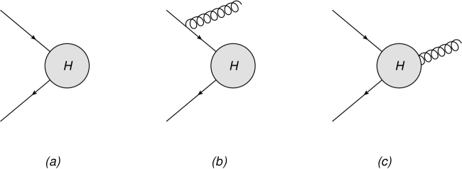
Figure 3: (a) Non-radiative amplitude with two incoming particles and a hard interaction ${\cal H}$; (b) external emission contribution; (c) internal emission contribution.

As shown for the first time in Ref. [28], external emissions can be described by generalised Wilson lines, which extend the definition given in Eq. (17) to next-to-leading power in the soft expansion. Along the lines of Eq. (18), we may write this operator in momentum space as [53]

$$F(p)\,=\,{\cal P}\exp\left[g_{s}{\bf T}^{a}\int\frac{d^{d}k}{(2\pi)^{d}}\,\tilde{A}_{\mu}^{a}(k)\left(\frac{p^{\mu}}{p\cdot k}-\frac{k^{\mu}}{2p\cdot k}+k^{2}\frac{p^{\mu}}{2(p\cdot k)^{2}}+{\rm i}k_{\nu}\frac{S^{\nu\mu}}{p\cdot k}\right)+\ldots\right]\,$$ (41)

for a generalised semi-infinite straight Wilson in the direction of four-momentum $p$. Here ${\bf T}^{a}$ is a colour generator in the appropriate representation, and $S^{\mu\nu}$ is the generator of Lorentz transformations for the parton under consideration, vanishing for scalar fields, while it is given by

$$\left(S^{\nu\mu}\right)_{\alpha\beta}\,\equiv\,{\Sigma^{\mu\nu}}_{\alpha\beta}\,=\,\frac{{\rm i}}{4}\left[\gamma^{\nu},\gamma^{\mu}\right]_{\alpha\beta}$$ (42)

for spin-$1/2$ fields, and

$$\left({S^{\nu\mu}}\right)_{\rho\sigma}\,\equiv\,{M^{\nu\mu}}_{\rho\sigma}\,=\,{\rm i}\left(\delta^{\nu}_{\rho}\,\delta^{\mu}_{\sigma}-\delta^{\nu}_{\sigma}\,\delta^{\mu}_{\rho}\right)$$ (43)

for vector fields. The first term in Eq. (41) corresponds to the eikonal Feynman rule of Eq. (18), and the remaining terms (suppressed by one power of the gluon momentum $k$) correspond to effective next-to-eikonal Feynman rules, describing the emission of next-to-soft gauge bosons [28]. The ellipsis in Eq. (41) refers to terms involving two gluons being emitted from the same point along the Wilson line, through seagull-type vertices. These vertices start contributing to the cross section at NNLO (either through double radiation, or one-loop corrections to single radiation), therefore, under mild assumptions, they cannot contribute at leading logarithmic accuracy at NLP (as was the case at LP). Indeed, our proposed resummation rests upon an amplitude-level factorisation theorem [27, 52, 53], which implies the existence of evolution equations, which in turn can be understood in terms of renormalisation of suitable operator matrix elements: the solution of evolution equations of this type always leads to a non-trivial pattern of exponentiation, with single logarithms in the exponent generating double logarithms in the cross section. Such a pattern of exponentiation implies that all leading logarithms are generated by the one-loop exponent. A test of this argument is provided by Ref. [36], where the exponentiation of leading logarithms at NLP was explictly tested at NNLO; finally, as a further check, we verify in Appendix C that next-to-soft Feynman rules for double radiation in Eq. (41) do no contribute to leading logarithms in the case of Drell-Yan production at two loops.

Let us now consider the contribution of internal emissions. When massive external particles are being considered, the hard interaction is analytic in the total momentum $K$ of the emitted radiation, and can safely be expanded about the soft limit $K^{\mu}\rightarrow 0$. One may then show, using Ward identities, that the effect of a single internal emission is given by derivatives of the non-radiative amplitude with respect to its external momenta. As has been noted in the context of the so-called next-to-soft theorems of Refs. [41, 40] , these derivatives can be organised in terms of the orbital angular momentum operator associated with each external leg, which, in momentum space, has the form

$$L^{(i)}_{\nu\mu}\,=\,{\rm i}\!\left(p_{i\nu}\frac{\partial}{\partial p_{i\mu}}-p_{i\mu}\frac{\partial}{\partial p_{i\nu}}\right)\,.$$ (44)

On each hard leg, this combines with the spin angular momentum contribution to construct the total angular momentum operator

$$S^{\nu\mu}\,\rightarrow\,S^{\nu\mu}+L^{\nu\mu}\,\equiv\,J^{\nu\mu}\,.$$ (45)

In Ref. [28], the orbital angular momentum contribution was not included in the generalised Wilson line operator of Eq. (41), despite the fact that it might make sense to do so, given that the internal and external emission contributions are not separately gauge-invariant, but instead combine into a gauge-invariant object, the total angular momentum. For practical purposes, however, it remains convenient to keep the orbital angular momentum separate, given that it involves derivatives which have yet to act on the hard interaction. How to keep track of such contributions will be discussed explicitly below.

Armed with the operator defined in Eq. (41), we may construct a next-to-soft function by analogy with the LP soft function of Eq. (16), as

$$\widetilde{\cal S}\left(z,Q^{2},\epsilon\right)\,=\,\frac{1}{N_{c}}\sum_{n,\,{\rm LP}}{\rm Tr}\left[\big{\langle}0\big{|}F^{\dagger}(p_{1})F(p_{2})\big{|}n\big{\rangle}\big{\langle}n\big{|}F^{\dagger}(p_{2})F(p_{1})\big{|}0\big{\rangle}\right]\delta\bigg{(}z-\frac{Q^{2}}{\hat{s}}\bigg{)}\,.$$ (46)

Here we have replaced the Wilson line operators in the LP soft function by their NLP counterparts, and the subscript in the sum over final states indicates that all phase space integrals are to be carried out with LP phase space only (i.e. with a measure of integration consisting of a product of single-gluon phase space integrals). Corrections to this will be considered in Section 3.2. Note also that all generalised Wilson lines are semi-infinite straight lines proceeding from the origin in position space. At NLP accuracy the cross section is sensitive to a potential non-zero initial position, but this is related to the derivative contributions above [28], which are to be dealt with separately. As was the case at LP, the next-to-soft function in Eq. (46) can be shown to exponentiate using replica trick arguments (see Appendix A). At NLP, however, we must carefully disentangle what this means, given that the generalised Wilson line of Eq. (41) is matrix-valued in the spin space of the external hard particles. As an example, consider the spin-$1/2$ case, and let us write the non-radiative amplitude with an incoming fermion and antifermion with explicit spin indices $\{\alpha,\beta\}$, as

$${\cal M}\,=\,\bar{v}_{\alpha}(p_{2})M^{\alpha\beta}u_{\beta}(p_{1})\,,$$ (47)

so that the spin matrix $M$ is defined by stripping off the initial state wave functions from the full amplitude. The next-to-soft function of Eq. (46) can then be explicitly written as a spin operator

$$\widetilde{\cal S}^{\,\,\alpha_{1}\alpha_{2}\bar{\alpha}_{1}\bar{\alpha}_{2}}_{\beta_{1}\beta_{2}\bar{\beta}_{1}\bar{\beta}_{2}}(z,Q^{2},\epsilon)\,=\,\frac{1}{N_{c}}\sum_{n,\,{\rm LP}}\big{\langle}0\big{|}F^{{\dagger}\,\bar{\alpha}_{1}}_{\bar{\beta}_{1}}(p_{1})\,F^{\,\bar{\alpha}_{2}}_{\bar{\beta}_{2}}(p_{2})\big{|}n\big{\rangle}\big{\langle}n\big{|}F^{{\dagger}\,{\alpha_{2}}}_{\beta_{2}}(p_{2})\,F^{\,\alpha_{1}}_{\beta_{1}}(p_{1})\big{|}0\big{\rangle}\,\delta\bigg{(}z-\frac{Q^{2}}{\hat{s}}\bigg{)}\,,$$ (48)

where the ordering of spinor indices is depicted in Figure 4.

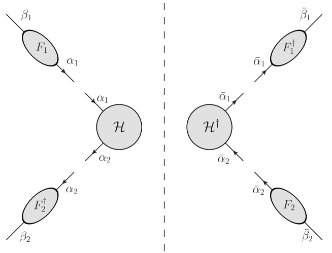
Figure 4: Labelling of spin indices for the squared amplitude, where $H$ is the hard function, and $F_{i}$ a generalised Wilson line.

The spin matrix $M^{\alpha\beta}$ in Eq. (47) factorises into a product of hard and next-to-soft factors, so that the integrated squared matrix element, dressed by arbitrary amounts of radiation from the next-to-soft function, can be written as

$$\int d\Phi^{(n+1)}\left|{\cal M}\right|^{2}\,=\,\widetilde{\cal S}^{\,\,\alpha_{1}\alpha_{2}\bar{\alpha}_{1}\bar{\alpha}_{2}}_{\beta_{1}\beta_{2}\bar{\beta}_{1}\bar{\beta}_{2}}(z,Q^{2},\epsilon)\int d\Phi^{(1)}\Big{[}\bar{v}^{\beta_{2}}(p_{2}){\cal H}_{\alpha_{1}\alpha_{2}}u^{\beta_{1}}(p_{1})\Big{]}\Big{[}\bar{u}^{\bar{\beta}_{1}}(p_{1}){\cal H}^{{\dagger}}_{\bar{\alpha}_{1}\bar{\alpha}_{2}}v^{\bar{\beta}_{2}}(p_{2})\Big{]}\,,$$ (49)

where $d\Phi^{(m)}$ denotes the $m$-particle Lorentz-invariant phase space measure, and the integration over the phase space of the heavy vector boson has been singled out, relying upon the factorisation of the $n$-body phase space at LP. An expression very similar to Eq. (49) holds for incoming particles of spin one, with spinors replaced by polarisation vectors, and spinor indices by vector indices.

The discussion so far applies strictly only to the case of massive external particles. When massless particles are involved, it is no longer true that the hard function ${\cal H}$ is analytic in the momentum carried by soft radiation: it develops logarithmic singularities due to the presence of collinear divergences. As discussed in the Introduction, this was first explored in a QED context in Ref. [27], which presented a factorisation formula at amplitude level, extending the Low-Burnett-Kroll theorem to include collinear effects. Similar ideas have recently been extended to full QCD [52, 53], and analysed using SCET [57, 96, 97, 75, 58, 59, 60, 61, 62, 67, 68, 69, 70, 71, 74, 98], while an alternative, first-principles, diagrammatic approach has been explored in Ref. [54]. Common to all these approaches is the factorisation of collinear contributions into universal functions, sensitive to the spin of the colliding particles but otherwise independent of the details of the hard scattering. More precisely, one may recall that, at leading power, collinear radiation is accounted for by means of jet-type functions, such as the parton distributions introduced in Eq. (12). At NLP, one must generalise this analysis, expressing radiative amplitudes in terms of new types of jet functions, describing soft emissions from collinearly enhanced configurations. The first such radiative jet function was proposed in Ref. [27], and was recently calculated at one loop in QCD for external quarks in Refs [52, 53], where it was used to reproduce known NLP threshold logarithms in Drell-Yan production at NNLO. The amplitude-level factorisation proposed in [52] is expected to apply only to annihilation processes involving two colliding hard partons producing colourless final states: on the other hand, the analysis of Ref. [54] (which focuses on scalar theories, but considers more general scattering processes), and the results of Refs. [57, 96, 97, 75] suggest that further types of jet emission function are necessary in QCD, which have yet to be calculated.

Importantly, for the purposes of the present paper, radiative jet functions can be ignored, since it can be shown that leading logarithms at NLP can only arise from momentum regions of integration that are already fully accounted for by the next-to-soft function introduced in Eq. (41). To illustrate this point, consider first, for comparison, the well-understood situation at leading power. In that case, threshold singularities, inducing non-analytic behaviour at $z\to 1$, are directly related to infrared singularities of the amplitude; these, in turn, arise from integrations of the relevant momentum components (‘normal variables’) near singular surfaces in momentum space, which can be completely characterised to all orders in perturbation theory by means of Landau equations and power counting techniques [99]. For massless theories, it can be shown in general that infrared singularities arise only from soft and collinear momentum configurations. At leading power, therefore, one finds that at $n$ loops there are precisely $2n$ normal variables that must be integrated with a logarithmic measure: in a suitable frame, these can be taken to be $n$ parton energies $E_{i}$, with a leading-power integration measure $dE_{i}/E_{i}$, and $n$ transverse momenta with respect to the directions defined by external particles, $k_{iT}$, with a leading-power integration measure $dk_{iT}/k_{iT}$. Threshold logarithms in general arise when different combinations of normal variables become small at different rates, but leading logarithms arise only with a very specific scaling, when all energies and transverse momenta are strongly ordered, say $E_{1}\ll\ldots\ll E_{n}$ and $k_{1T}\ll\ldots\ll k_{nT}$. In that limit, at LP, the $2n$ logarithmic integrations yield contributions of the form $\ln^{2n-1}(1-z)/(1-z)$, since the last logarithmic integration must not performed when computing $d\hat{\sigma}/dz$. At NLP, either the phase-space measure or the squared matrix element provide a single power of one of the normal variables, so that only $2n-1$ momentum components need be integrated with a logarithmic measure. Once again, leading logarithms will arise from the configuration where the remaining normal variables are strongly ordered, with $2n-1$ integrations leading to contributions of the form $\ln^{2n-1}(1-z)$, while the $z$ integration will not introduce further singularities at NLP. Now, two possibilities arise. On the one hand, the normal variable whose integration has become non-singular can be a transverse momentum, in which case the corresponding parton is soft, but not strictly collinear: this configuration is accounted for by the leading-power soft function, which contains ‘wide-angle’ soft gluons. On the other hand, the suppressed variable can be an energy: in this case, all transverse momenta must be strongly ordered; such next-to-soft, collinear configurations are accounted for by the next-to-soft function defined in Eq. (46). Notice that radiative jet functions such as the one computed in [52] also contain the next-to-soft, collinear configuration: this, however, contributes to a double counting that must be explicitly subtracted, either by introducing eikonal jets, as done in Eq. (12), or by defining an appropriate counterterm, as done for example in Ref. [53]. The subtracted radiative jet function then contains only hard collinear configurations for all radiated partons, and cannot contribute at leading logarithmic accuracy.

An explicit example and test of the above discussion is provided in Ref. [53], where the non-abelian radiative jet function for quarks was computed at one-loop order, and the overlap between (next-to-)soft and collinear emissions was explicitly identified. Furthermore, a large class of (N)LP threshold effects has been calculated in Drell-Yan production at NNLO [65] and N³LO [66] using the method of regions [100, 101, 102], which allows for a precise identification of the (next-to)soft and/or collinear origin of all contributions to the cross section. The role of hard collinear effects is indeed found in these studies to be associated with NLL terms and beyond , while all LL contributions can be traced to the (next-to)soft function, if the results are recast in the present framework. Notice that, as discussed above, upon exponentiation leading logarithms at NLP must be generated by one-loop contributions: the results of [53, 65, 66] therefore provide a complete test of our argument for the Drell-Yan process.

To summarise, NLP contributions to squared matrix elements can be categorised into two main types, as follows.

1. (Next-to-)soft emissions. These are captured by the next-to-soft function, defined in terms of generalised Wilson lines in Eq. (46), together with the orbital angular momentum contributions associated with internal emissions in Figure 3. As at LP, the next-to-soft function exponentiates (see Appendix A).

2. Collinear contributions. These are described by radiative jet functions, which overlap with the next-to-soft function. Upon removing the double counting, the remaining collinear effects do not contribute at LL accuracy.

In this section, we have discussed the second term on the right-hand side of Eq. (40), and argued that the next-to-soft function underlies all contributions to the NLP matrix element that can result in LL terms in the cross-section. This is only part of the story: we must also check whether or not LL terms can arise from the LP matrix element, once correlations between radiated gluons (a NLP effect) are included. This is the subject of the following section.

3.2 Corrections to the LP phase space

The third term in Eq. (40) consists of the LP matrix element integrated over the NLP phase space. To see whether or not this term can give LL contributions at NLP, it is sufficient to take the LL contribution to the LP matrix element at each order, and then to evaluate the phase space integral up to NLP order. The LL contributions to the matrix element have already been discussed in Section 2, and involve exponentiating the NLO eikonal squared matrix element. This generates terms with $n\geq 1$ gluon emissions, and, according to Eq. (16), one must then integrate each such term over the $n$-gluon phase space. Considering all possible contributions to an $n$-gluon final state yields a squared matrix element of the form

$$|{\cal M}|^{2}_{\rm LP,n}\,=\,f\big{(}\alpha_{s},\epsilon,\mu^{2}\big{)}\,\prod_{i=1}^{n}\frac{p_{1}\cdot p_{2}}{p_{1}\cdot k_{i}\,p_{2}\cdot k_{i}}\,,$$ (50)

where the prefactor $f(\alpha_{s},\epsilon,\mu^{2})$ collects coupling dependence, possible poles in $\epsilon$ due to the integration over loop momenta, and combinatorial factors from the exponentiation of the squared matrix element. The explicit form of this function is irrelevant for what follows. We must now integrate Eq. (50) over the $(n+1)$-body phase space, consisting of $n$ gluons, as well as the electroweak vector boson that defines the final state at LO. The integration measure is given by

$$d\Phi^{(n+1)}\,=\,\bigg{[}\prod_{i=1}^{n}\int\frac{d^{d}k_{i}}{(2\pi)^{d-1}}\,\delta_{+}(k_{i}^{2})\bigg{]}\delta\bigg{(}1-z-2\sum_{i=1}^{n}\frac{k_{i}\cdot(p_{1}+p_{2})}{\hat{s}}+2\sum_{i<j}\frac{k_{i}\cdot k_{j}}{\hat{s}}\bigg{)}\,,$$ (51)

where the integration of the vector boson momentum has already been carried out, using the overall momentum conservation $\delta$ function. In order to compute the integral, it is particularly convenient to use the Sudakov decomposition of Eq. (24) for each momentum $k_{i}$. One finds

$$\int d\Phi^{(n+1)}|{\cal M}|^{2}_{\rm LP,n} = f(\alpha_{s},\epsilon,\mu^{2})\left[\prod_{i=1}^{n}\frac{1}{\pi\hat{s}}\int_{0}^{\infty}\frac{dk_{i+}}{k_{i+}}\int_{0}^{\infty}\frac{dk_{i-}}{k_{i-}}\int\frac{d^{d-2}\mbox{\boldmath$k$}_{iT}}{(2\pi)^{d-2}}\,\delta(k_{i-}k_{i+}-\mbox{\boldmath$k$}_{iT}^{2})\right]$$ (52)

$$\times\,\delta\bigg{(}1-z-\frac{(k_{i+}+k_{i-})}{\sqrt{\hat{s}}}+2\sum_{i<j}\frac{k_{i}\cdot k_{j}}{\sqrt{\hat{s}}}\bigg{)}\,,$$

where we absorbed the $\theta$ functions from the factors $\delta_{+}(k_{i}^{2})$ into the integration limits for $k_{i\pm}$. In order to proceed, we can represent the $\delta$ function in the second line of Eq. (52) using

$$\delta(x)\,=\,\int_{-{\rm i}\infty}^{{\rm i}\infty}\,\frac{dT}{2\pi{\rm i}}\,{\rm e}^{Tx}\,.$$ (53)

We may then rewrite Eq. (52) as

$$\int d\Phi^{(n+1)}|{\cal M}|^{2}_{\rm LP,n} = f(\alpha_{s},\epsilon,\mu^{2})\int_{-{\rm i}\infty}^{{\rm i}\infty}\frac{dT}{2\pi{\rm i}}\,{\rm e}^{T(1-z)}\Bigg{[}\prod_{i=1}^{n}\frac{1}{\pi\hat{s}}\int_{0}^{\infty}\frac{dk_{i+}}{k_{i+}}\int_{0}^{\infty}\frac{dk_{i-}}{k_{i-}}$$

$$\times \!\!\!\int\frac{d^{d-2}\mbox{\boldmath$k$}_{iT}}{(2\pi)^{d-2}}\,\delta(k_{i-}k_{i+}-\mbox{\boldmath$k$}_{iT}^{2})\,{\rm e}^{-\frac{T(k_{i+}+k_{i-})}{\sqrt{\hat{s}}}}\Bigg{]}\bigg{[}1+\frac{2T}{\hat{s}}\sum_{i<j}k_{i}\cdot k_{j}+{\cal O}(T^{2})\bigg{]}\,,$$

where in the second line we Taylor-expanded the term in the exponent that is quadratic in soft momentum, anticipating that higher order contributions in $T$ in the last line will correspond to subleading powers of $(1-z)$ in the final result. We will verify this fact later, but, for the moment, note that the term at ${\cal O}(T)$ corresponds to a phase space correlation between pairs of gluons that is absent at LP. Thus, this term constitutes the “NLP phase space” correction referred to in Eq. (40). In the Sudakov decomposition, the dot product of gluon momenta reads

$$k_{i}\cdot k_{j}\,=\,\frac{k_{i+}k_{j-}+k_{i-}k_{j+}}{2}-\mbox{\boldmath$k$}_{iT}\cdot\mbox{\boldmath$k$}_{jT}\,.$$ (55)

The term involving the transverse momenta leads to an odd integrand in each $\mbox{\boldmath$k$}_{iT}$ in Eq. (3.2), and will therefore give a vanishing contribution to the final result. We can then carry out the remaining transverse momentum integrals to obtain

$$\int d\Phi^{(n+1)}|{\cal M}|^{2}_{\rm LP,n} = f(\alpha_{s},\epsilon,\mu^{2})\int_{-{\rm i}\infty}^{{\rm i}\infty}\frac{dT}{2\pi{\rm i}}\,{\rm e}^{T(1-z)}\Bigg{[}\prod_{i=1}^{n}\frac{\Omega_{d-2}}{\hat{s}(2\pi)^{d-1}}\int_{0}^{\infty}dk_{i+}\int_{0}^{\infty}dk_{i-}$$

$$\left(k_{i+}\,k_{i-}\right)^{(d-6)/2}{\rm e}^{-\frac{T(k_{i+}+k_{i-})}{\sqrt{\hat{s}}}}\Bigg{]}\bigg{[}1+\frac{T}{\hat{s}}\sum_{i<j}\left(k_{i+}k_{j-}+k_{i-}k_{j+}\right)+{\cal O}(T^{2})\bigg{]}\,.$$

Next, the $k_{i\pm}$ integrals can be straightforwardly carried out to give

$$\int d\Phi^{(n+1)}|{\cal M}|^{2}_{\rm LP,n} = f(\alpha_{s},\epsilon,\mu^{2})\,\frac{\Omega_{d-2}^{n}\,\hat{s}^{n(d-6)/2}}{(2\pi)^{n(d-1)}}\int_{-{\rm i}\infty}^{{\rm i}\infty}\frac{dT}{2\pi{\rm i}}\,{\rm e}^{T(1-z)}$$

$$\times\,\Bigg{[}\frac{1}{T^{n(d-4)}}\,\Gamma^{2n}\bigg{(}\frac{d-4}{2}\bigg{)}+\,\frac{n(n-1)}{T^{n(d-4)+1}}\,\Gamma^{2n-2}\bigg{(}\frac{d-4}{2}\bigg{)}\,\Gamma^{2}\bigg{(}\frac{d-2}{2}\bigg{)}+{\cal O}\bigg{(}\frac{1}{T^{n(d-4)+2}}\bigg{)}\Bigg{]}\,.$$

The integral in $T$ is recognisable as an inverse Laplace transform, which yields the result

$$\int d\Phi^{(n+1)}|{\cal M}|^{2}_{\rm LP,n} = f(\alpha_{s},\epsilon,\mu^{2})\,\frac{\Omega_{d-2}^{n}\,\hat{s}^{n(d-6)/2}}{(2\pi)^{n(d-1)}}\,\frac{\Gamma^{2n}[(d-4)/2]}{\Gamma[n(d-4)]}\,(1-z)^{n(d-4)-1}$$ (58)

$$\hskip 14.22636pt\times\,\bigg{\{}1+\frac{(n-1)(d-4)(1-z)}{4}+{\cal O}\big{[}(1-z)^{2}\big{]}\bigg{\}}\,.$$

Note that the terms ${\cal O}(T^{2})$ we have neglected in expanding the exponential factor in Eq. (3.2) give subleading power corrections in $(1-z)$, justifying the approximation made above. Eq. (58) is the final result of integrating the LP contribution to the matrix element responsible for LL terms, with the multigluon phase-space measure expanded to NLP order. The second term in the last line of Eq. (58) is the desired NLP correction, as can be seen by the fact that it is suppressed by a single power of $(1-z)$. Furthermore, it contains an explicit factor of $d-4=-2\epsilon$, which directly implies that the phase space correction does not affect LL terms, which are associated with the most singular poles in $\epsilon$.

In summary, we have shown that the third term in Eq. (40), consisting of the LP matrix element dressed with NLP phase space corrections, does not contribute to LL terms at NLP order. It can thus be neglected for the purposes of this paper. Combining this observation with the results of the previous section, we now have everything we need to perform an explicit resummation of LL NLP threshold logarithms in Drell-Yan production. We turn to this task in the next section.

3.3 Resummation of leading NLP logs in Drell-Yan production

In the previous sections, we have seen that LL contributions at NLP level are governed by next-to-soft radiation. This in turn is captured by the next-to-soft function defined in Eq. (46), possibly complemented by contributions involving the orbital angular momentum of each incoming parton. In this section, we apply these ideas to resum LL NLP terms in Drell-Yan production. While clearly very interesting for its own sake, this example is also a useful warm-up case: first, it will allow us to make contact with the LP treatment of Section 2; furthermore, in this case the hard interaction is especially simple, so that its derivatives with respect to the external momenta vanish at leading order. Thus, we do not have to worry about orbital angular momentum contributions at LL accuracy, and it is sufficient to calculate the next-to-soft function. Once this has been calculated for single radiation, it may be exponentiated (as at LP), yielding the resummation formula that we are seeking.

For the first steps of our derivation, we do not need to specify the final-state particle content of the process we are studying. Rather, we will consider a general hard interaction ${\cal H}$ connecting to an incoming $q\bar{q}$ pair, such that the LO amplitude is given by Eq. (47). Representative diagrams contributing to the squared amplitude arising from the next-to-soft function at NLO, Eq. (49), are shown in Figure 5.

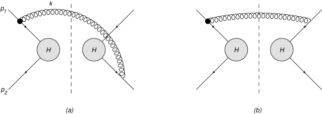
Figure 5: Diagrams contributing to a squared amplitude with a $q\bar{q}$ initial state, arising from the next-to-soft function $\tilde{S}$ acting on the LO hard interaction ${\cal H}$, as in Eq. (49). Further diagrams are obtained by reflection about the final state cut, or by interchanging $p_{1}\leftrightarrow p_{2}$.

We may directly evaluate them using the Feynman rules arising from Eq. (41). First, we may note that contributions involving $k^{2}$ vanish, since the radiated gluon is on shell. Next, it is convenient to combine the scalar-like and spin-dependent emission vertices as

$$\frac{k^{\mu}}{2p_{i}\cdot k}-{\rm i}k_{\nu}\frac{\Sigma^{\nu\mu}}{p_{i}\cdot k}\,=\,\frac{\not\!{k}\gamma^{\mu}}{2p_{i}\cdot k}\,.$$ (59)

Then, the diagrams of Figure 5 yield a NLP contribution

$$\left|{\cal M}\right|^{2}_{\rm NLP,\,(a)+(b)} = 2g_{s}^{2}C_{F}\left(\frac{p_{1}^{\mu}}{p_{1}\cdot k}-\frac{p_{2}^{\mu}}{p_{2}\cdot k}\right){\rm Tr}\left[\not\!{p}_{2}{\cal H}\left(\frac{\not\!{k}\gamma^{\mu}}{2p_{1}\cdot k}\right)\not\!{p}_{1}{\cal H}^{\dagger}\right]$$ (60)

$$= -\,\frac{g_{s}^{2}C_{F}}{p_{1}\cdot k\,p_{2}\cdot k}\,{\rm Tr}\left[\not\!{p}_{2}{\cal H}\not\!{k}\not\!{p}_{2}\not\!{p}_{1}{\cal H}^{\dagger}\right]\,,$$

where a factor of two for complex conjugate diagrams has already been included. In order to extract the LO squared amplitude, we may use an argument similar to one presented recently in Ref. [64]. Writing the decomposition (cf. Eq. (24))

$$\not\!{k}\,=\,\frac{p_{2}\cdot k}{p_{1}\cdot p_{2}}\not\!{p_{1}}+\frac{p_{1}\cdot k}{p_{1}\cdot p_{2}}\not\!{p_{2}}+\not\!{k}_{T}\,,$$ (61)

and substituting into Eq. (60) reveals that the term involving transverse momentum occurs linearly in the squared matrix element, leading to an odd integrand which vanishes upon integrating over $k_{T}$. This contribution can thus be ignored, leading effectively to the expression

$$\left|{\cal M}\right|^{2}_{\rm NLP,\,(a)+(b)}\,=\,-\,\frac{2g_{s}^{2}C_{F}}{p_{1}\cdot k}\,{\rm Tr}\left[\not\!{p}_{2}{\cal H}\not\!{p}_{1}{\cal H}^{\dagger}\right]\,.$$ (62)

Notably, in Eq. (62) the LO squared matrix element is factored out. Combining this with diagrams obtained from those of Figure 5 by interchanging $p_{1}$with $p_{2}$, summing over spins and colours, and dividing out the LO cross section one easily obtains an expression for the real emission contribution to the one-loop next-to-soft function. Notice that at NLP singularities as $z\rightarrow 1$ are integrable: thus, there is no need to combine real emission with virtual corrections in order to generate LL contributions, and the NLP soft function reads

$${\cal S}_{\rm NLP}^{(1)}\left(z,Q^{2},\epsilon\right) = -2\mu^{2\epsilon}g_{s}^{2}\,C_{F}\int\frac{d^{d}k}{(2\pi)^{d-1}}\,\delta_{+}(k^{2})\,\delta\!\left(1-z-\frac{2k\cdot(p_{1}+p_{2})}{\hat{s}}\right)$$ (63)

$$\hskip 85.35826pt\times\left(\frac{1}{p_{1}\cdot k}+\frac{1}{p_{2}\cdot k}\right)\,.$$

The integration over the real gluon phase space can be carried out straightforwardly using the Sudakov decomposition of Eq. (24), and the subsequent change of variables in Eq. (29), with the result

$${\cal S}_{\rm NLP}^{(1)}\left(z,Q^{2},\epsilon\right)\,=\,-\frac{2\alpha_{s}C_{F}}{\pi}\left(\frac{\bar{\mu}^{2}}{Q^{2}}\right)^{\epsilon}\frac{e^{\epsilon\gamma_{E}}\Gamma^{2}(-\epsilon)}{\Gamma(1-\epsilon)\Gamma(-2\epsilon)}\,(1-z)^{-2\epsilon}\,.$$ (64)

Taking the Mellin transform we find

$${\cal S}_{\rm NLP}^{(1)}\left(N,Q^{2},\epsilon\right) \equiv \int_{0}^{1}dz\,z^{N-1}{\cal S}_{\rm NLP}^{(1)}\left(z,Q^{2},\epsilon\right)$$ (65)

$$= -\frac{2\alpha_{s}C_{F}}{\pi}\left(\frac{\bar{\mu}^{2}}{Q^{2}}\right)^{\epsilon}\frac{e^{\epsilon\gamma_{E}}\Gamma(-\epsilon)\Gamma(N)}{\Gamma(1-2\epsilon+N)}$$

$$= \frac{2\alpha_{s}C_{F}}{\pi}\left(\frac{\bar{\mu}^{2}}{Q^{2}}\right)^{\epsilon}\frac{1}{N}\left[\frac{1}{\epsilon}+2\psi^{(0)}(N+1)+2\gamma_{E}\right]+{\cal O}(\epsilon)\,.$$

The leading behaviour as $N\rightarrow\infty$ is

$${\cal S}_{\rm NLP}^{(1)}\left(N,Q^{2},\epsilon\right)\,=\,\frac{2\alpha_{s}C_{F}}{\pi}\left(\frac{\bar{\mu}^{2}}{Q^{2}}\right)^{\epsilon}\left[\,\frac{1}{\epsilon}\,\frac{1}{N}+\frac{2\log N}{N}+\ldots\right]\,,$$ (66)

where the ellipsis denotes terms which are non-singular in $\epsilon$ and non-logarithmic in $N$, as well as terms suppressed by further powers of $N$. We see that the NLP soft function generates contributions which are suppressed by (at least) a single power of $N$ compared to LP, as expected. Eq. (66) must now be combined with the LP soft function given Eq. (39), which itself includes subleading terms in $N$ space arising from the Mellin transformation from $z$ space. The result is

$${\cal S}_{\rm LP+NLP}\left(N,Q^{2},\epsilon\right)\,=\,\frac{2\alpha_{s}C_{F}}{\pi}\left(\frac{\bar{\mu}^{2}}{Q^{2}}\right)^{\epsilon}\left[\frac{1}{\epsilon}\left(\log N+\frac{1}{2N}\right)+\log^{2}N+\frac{\log N}{N}\right]\,.$$ (67)

As explained above, we may directly exponentiate Eq. (67), and combine it with the LO cross-section. Furthermore, the collinear pole can be absorbed in the quark distributions, for which we again use the $\overline{\rm MS}$ factorisation scheme. To this end, we generalise Eq. (37) to

$$q_{\rm LL,\,NLP}\!\left(N,Q^{2}\right)\,=\,q_{N}(Q^{2})\exp\left[\frac{\alpha_{s}C_{F}}{\pi}\,\frac{1}{\epsilon}\left(\log N+\frac{1}{2N}\right)\right]\,,$$ (68)

and similarly for the antiquark. Note that it is important in Eq. (68) that we correctly kept track of subleading terms in the Mellin transform of the LP soft function. The cross-section at NLP in the threshold expansion and at LL accuracy then becomes

$$\left.\int_{0}^{1}d\tau\,\tau^{N-1}\,\frac{d\sigma_{\rm DY}}{d\tau}\right|_{\rm LL,\,NLP} = \sigma_{0}(Q^{2})\,q_{\rm LL,\,NLP}\!\left(N,Q^{2}\right)\,\bar{q}_{\rm LL,\,NLP}\!\left(N,Q^{2}\right)$$ (69)

$$\quad\times\exp\left[\frac{2\alpha_{s}C_{F}}{\pi}\left(\log^{2}\!N+\frac{\log N}{N}\right)\right]\,.$$

Upon expanding the exponential factor in powers of $\alpha_{s}$, we may now perform the inverse Mellin transform of the partonic cross-section order by order, using the results of Appendix B, to get

$$\Delta(z,Q^{2})|_{\rm LL,\,NLP}\,=\,\left(\frac{2\alpha_{s}C_{F}}{\pi}\right)^{m}\!\!\frac{1}{(m-1)!}\left[2\left(\frac{\log^{2m-1}(1-z)}{1-z}\right)_{+}\!-2\log^{2m-1}(1-z)\right]\,.$$ (70)

This is in complete agreement with (and indeed provides an independent proof of) the result of Ref. [31], which argued (consistently with previous observations [23, 36]) that the LL NLP terms at any order have a coefficient which is always the negative of that of the corresponding leading logarithmic plus distribution. The origin of this phenomenon can be traced to the coefficient of the $\epsilon$ pole in Eq. (66). Given that this pole represents a collinear singularity that must be absorbed in the parton distributions, it must emerge from the NLP contribution to the LO DGLAP splitting kernel that governs such terms. More specifically, the collinear poles in the NLO Drell-Yan cross-section have the form (see for example Ref. [103])

$$-\frac{2}{\epsilon}\,P_{qq}^{(0)}\,,$$ (71)

where the factor of 2 arises from having collinear singularities associated with either of the incoming partons. The splitting function can be expanded near threshold as

$$P^{(0)}_{qq}(z)\,=\,\frac{\alpha_{s}}{2\pi}\,C_{F}\left[\frac{2}{(1-z)_{+}}-2+\ldots\right]\,.$$ (72)

where the second term gives the NLP contribution in $z$-space, whose Mellin transform is

$$\int_{0}^{1}dzz^{N-1}\,\left.P^{(0)}_{qq}(z)\right|_{\rm NLP}\,=\,-\frac{\alpha_{s}C_{F}}{\pi}\frac{1}{N}\,.$$ (73)

We thus expect the collinear pole of the NLP contribution to the next-to-soft function in Mellin space to be given by

$$\frac{2\alpha_{s}\,C_{F}}{\pi}\,\frac{1}{N}\,\frac{1}{\epsilon}\,,$$ (74)

which is indeed observed in Eq. (66). We see that the next-to-soft function generates the correct NLP correction to the splitting kernel as expected. This in turn dictates the LL behaviour in the finite part: indeed, in $z$-space, this contribution arises completely from an overall $\epsilon$-dependent power of $(1-z)$, dressing the pole term. Thus, ensuring that the NLP behaviour of the pole term is correct is sufficient to describe also the finite part. Note that the fact that all NLP information in the DGLAP splitting function is correctly generated by the next-to-soft expansion provides a test of the statement made earlier, that all LL threshold effects at (N)LP arise from radiation that is (next-to) soft, in addition to being collinear. This in turn confirms that, at LL accuracy, one may neglect radiative jet functions [27, 52, 53, 54, 55, 56].

Eq. (69) resums the leading-logarithmic behaviour of the Drell-Yan cross section at LP and NLP in the threshold expansion: it completely agrees with expectations from the literature [36, 31], and thus with the recent SCET analysis of Ref. [75], which cross-checked against the same references. We emphasise that, of course, at leading power there is no need to limit the resummation to leading logarithms: this was done in Eq. (69) only for simplicity, and to underline the close connection between leading logarithms at LP and NLP. Indeed, because of the link discussed above between NLP leading logarithms and the DGLAP kernels, it is straightforward to incorporate our results in the standard LP resummation formalism: it is sufficient to include NLP terms in the quark splitting function. This was argued to be appropriate in Refs.[23, 36, 31], and, with the mild assumptions discussed in Section 3.1, it is now proven. For completeness, we include here the general resummation ansatz introduced in Ref. [36], which implements this change in the classic threshold resummation formula of [6, 7, 8], together with other proposed modifications that have effects on subleading NLP logarithms. In Mellin space, the result of Ref. [36] for the Drell-Yan process can be written as

$$\ln\Big{[}\Delta(N,Q^{2})\Big{]} = F_{\rm DY}\left[\alpha_{s}(Q^{2})\right]+\int_{0}^{1}\,dz\,z^{N-1}\,\Bigg{\{}\frac{1}{1-z}\,D\left[\alpha_{s}\left(\frac{(1-z)^{2}Q^{2}}{z}\right)\right]$$ (75)

$$+ 2\,\int_{Q^{2}}^{(1-z)^{2}Q^{2}/z}\,\frac{dq^{2}}{q^{2}}\,P_{qq}^{\rm\,LP+NLP}\Big{[}z,\alpha_{s}(q^{2})\Big{]}\Bigg{\}}_{+}\,.$$

In Eq. (75), $D(\alpha_{s})$ is the well-known LP wide-angle soft function for the Drell-Yan process, which has been computed up to three loops in [104, 105, 106, 107]; $F_{\rm DY}(\alpha_{s})$ resums $N$-independent contributions following Ref. [2]; $P_{qq}^{\rm\,LP+NLP}(z,\alpha_{s})$ is the soft expansion of the DGLAP splitting function up to NLP, order by order in perturbation theory, which was derived in [36] starting from the results of Ref. [108]; furthermore, the ‘plus’ prescription is defined to apply only to LP contributions, that are singular as $z\to 1$. Leading NLP logarithms in Eq. (75) are generated by the one-loop NLP contribution to $P_{qq}^{\rm\,LP+NLP}$, as discussed in this Section. Higher-order terms in the NLP splitting function will contribute to, but not exhaust, subleading NLP logarithms; indeed, the shifts in the phase space boundary and in the argument of the coupling, proposed in Eq. (75), and corresponding to a NLP-accurate definition of the soft scale of the process, also contribute to subleading logarithms at NLP. In Ref. [36], the accuracy of Eq. (75) was tested by comparing its expansion to NNLO with existing exact results: as expected from our current discussion, leading NLP logarithms are exactly predicted; furthermore, one observes that next-to-leading NLP logarithms are predicted very accurately, and they mostly arise from the NLO contribution to the NLP splitting function. The small discrepancy arising at this level of accuracy (NLL at NLP) between the resummation and the finite order result is the first footprint of the need to include radiative jet functions at NLP.

3.4 A brief comparison with the SCET approach

In Section 3.3, we have achieved the resummation of leading NLP logarithms (jointly with all LP logarithms) by applying essentially diagrammatic arguments, based on the previous analysis of Ref. [28], summarised here in Appendix A. Clearly, these diagrammatic arguments are in turn based on an underlying factorisation [52, 53], but the argument for resummation is greatly simplified by the diagrammatic exponentiation properties of the (next-to-)soft function. Recently, the resummation of these same contributions has been achieved for the Drell-Yan process also within an effective field theory approach based on SCET [75] (see also Ref. [74]). In this section, we briefly compare our methods with the SCET analysis, whose physics must ultimately be equivalent.

The SCET approach relies upon a factorisation of the partonic cross section $\Delta(z)$, obtained by expanding the Drell-Yan QCD current into operators defined in terms of effective soft and collinear fields, with a different collinear sector associated with each external parton. Hard modes of the field contribute through short-distance coefficients of SCET operators, which can be obtained by matching to full QCD. Under the assumption that Glauber-type modes of the gluon field do not contribute to the relevant observable, soft and collinear modes can be factorised into (universal) matrix elements, which define collinear and soft functions, in direct correspondence with the jet and the soft functions emerging from the diagrammatic approach considered in this work.

Restricting to the terms relevant for the resummation of leading logarithms up to NLP, the momentum-space SCET factorisation for the partonic cross-section $\Delta$ introduced in Eq. (6) takes the form

$$\Delta(z)\,=\,H(Q^{2},\mu_{h})\,Q\,\bigg{[}S_{\rm DY}\big{(}Q(1-z),\mu_{s}\big{)}\,-\,\frac{4}{Q}\int\!d\omega\,S_{2\xi}(Q(1-z),\omega,\mu_{s})\bigg{]}\,,$$ (76)

where $H(Q^{2},\mu_{h})$ is the hard function, $S_{\rm DY}$ represents the leading-power soft function, equivalent to the one defined in Eq. (16), and $S_{2\xi}$ represents that part of the NLP soft function that contributes at leading logarithmic accuracy, to be compared with LL form of ${\cal S}_{\rm NLP}$ in Section 3.3. In Eq. (76) no collinear functions appear explicitly, since hard collinear modes contribute only starting at NLL accuracy. This conclusion is obtained within SCET by an analysis of all possible operators contributing at NLP, and confirmed a posteriori, as we will see below.

Each function in the SCET factorisation depends on a characteristic momentum scale: $\mu_{h}\sim Q$ for the hard function, and $\mu_{s}\sim Q(1-z)$ for the soft functions. Independence of physical observables on the factorisation scales yields a renormalisation group equation, which can be solved to resum the large logarithms. To this end, it is appropriate to evolve the hard and soft functions in Eq. (76) to a common scale, which in Ref. [75] is chosen to be $\mu_{c}\sim Q\sqrt{1-z}$. To LL accuracy, the evolved hard and soft functions can be written as [75]

$$\left.H(Q^{2},\mu_{c})\right|_{\rm LL} = \exp\big{[}4\,E_{\rm LL}(\mu_{h},\mu_{c})\big{]}\,H(Q^{2},\mu_{h})\,,$$

$$\left.S_{2\xi}(Q(1-z),\omega,\mu_{c})\right|_{\rm LL} = \frac{2C_{F}}{\beta_{0}}\,\ln\frac{\alpha_{s}(\mu_{c})}{\alpha_{s}(\mu_{s})}\,\,\exp\big{[}-4\,E_{\rm LL}(\mu_{s},\mu_{c})\big{]}\theta(1-z)\delta(\omega)\,.$$ (77)

Here the evolution factor $E_{\rm LL}$ resums the logarithms, and can be expressed in terms of the strong coupling evaluated at different scales, as

$$E_{\rm LL}(\nu,\mu)\,=\,-\int\limits_{\alpha_{s}(\nu)}^{\alpha_{s}(\mu)}\!d\alpha\,\frac{\Gamma_{\rm cusp}(\alpha)}{\beta(\alpha)}\int\limits_{\alpha_{s}(\nu)}^{\alpha}\frac{d\alpha^{\prime}}{\beta(\alpha^{\prime})}\,\stackrel{{\scriptstyle\rm LL}}{{=}}\,\frac{C_{F}}{\beta_{0}^{2}}\frac{4\pi}{\alpha_{s}(\nu)}\left(1-\frac{\alpha_{s}(\nu)}{\alpha_{s}(\mu)}+\ln\frac{\alpha_{s}(\nu)}{\alpha_{s}(\mu)}\right)\,,$$ (78)

where we have introduced the QCD cusp anomalous dimension and beta function. Using the fact that, for Drell-Yan production, $H(Q^{2},\mu_{h})=1+{\cal O}(\alpha_{s})$, one can compute $\Delta(z)$ in Eq. (76) with all factors evaluated at the scale $\mu_{c}$. In order to avail oneself of the standard collinear factorisation machinery, one must then evolve both $\Delta(z)$ and the parton distributions to a generic factorisation scale $\mu$, exploiting the RG invariance of the physical cross-section. One then finds

$$\Delta^{\rm LL}_{\rm NLP}(z,\mu)\,=\,-\,\frac{8C_{F}}{\beta_{0}}\,\exp\big{[}4\,E_{\rm LL}(\mu_{h},\mu)-4\,E_{\rm LL}(\mu_{s},\mu)\big{]}\,\ln\frac{\alpha_{s}(\mu)}{\alpha_{s}(\mu_{s})}\,.$$ (79)

The fact that the evolution of parton distributions (dictated by DGLAP splitting functions) is consistent at LL accuracy with the evolution of the partonic cross section to a generic scale provides an independent check of the fact that collinear function (absent in Eq. (76)) cannot contain leading NLP logarithms. This is directly analogous to the observation made here in Section 3.3, where we noted that the effect of including next-to-soft radiation led to reproducing the NLP contribution to the DGLAP kernels, testing our arguments for not including radiative jet functions in the derivation leading to Eq. (69).

In order to compare the result in Eq. (79) with Eq. (70), one needs to expand the ratios of running couplings in Eq. (79) and Eq. (78) in powers of $\alpha_{s}(\mu)$. When this is done, the NLP term in Eq. (79) reduces to

$$\Delta^{\rm LL}_{\rm NLP}(z,\mu)\,=\,-4\,\frac{\alpha_{s}}{\pi}C_{F}\,\exp\left[-\frac{2\alpha_{s}C_{F}}{\pi}\ln^{2}\frac{\mu}{\mu_{h}}\right]\,\exp\left[\frac{2\alpha_{s}C_{F}}{\pi}\ln^{2}\frac{\mu}{\mu_{s}}\right]\ln\frac{\mu_{s}}{\mu}\,\theta(1-z)\,.$$ (80)

Upon setting the hard and soft scales to their natural values, $\mu_{h}=Q$ and $\mu_{s}=Q(1-z)$, and choosing (as above) a factorisation scale of $\mu=Q$, we find

$$\Delta^{\rm LL}_{\rm NLP}(z,\mu)\,=\,-4\,\frac{\alpha_{s}}{\pi}C_{F}\exp\left[\frac{2\alpha_{s}C_{F}}{\pi}\ln^{2}(1-z)\right]\ln(1-z)\,\theta(1-z)\,,$$ (81)

which is readily seen to be equivalent to Eq. (70).

3.5 Resummation for general quark-initiated colour-singlet production

In section 3.3 we have seen how to resum the highest power of NLP logs, for the specific case of Drell-Yan production. In fact, the result can easily be generalised to the production of $N$ colour singlet particles (which may be loop-induced at leading order), with a $q\bar{q}$ initial state. Crucial to our arguments will be exponentiation of the next-to-soft function in terms of webs [28, 29], which implies that the next-to-soft function has the schematic form

$${\cal S}_{\rm NLP}\,=\,\exp\left[\sum_{i}W_{\rm LP}^{(i)}+\sum_{j}W_{\rm NLP}^{(j)}\right]\,,$$ (82)

where the first sum is over leading power webs composed with eikonal Feynman rules, and the second sum is over next-to-leading power webs, containing eikonal Feynman rules with at most one next-to-eikonal vertex. Next, we may note, as was remarked in Refs. [28, 29], that if we are only interested in NLP terms in the final result for the cross-section, we do not in fact have to exponentiate the NLP webs: upon expanding Eq. (82) in powers of the coupling, quadratic and higher powers of the NLP term will give NNLP contributions and beyond. Thus, we may formally replace Eq. (82) with the equivalent expression (up to NLP level)

$${\cal S}_{\rm NLP}\,=\,\exp\left[\sum_{i}W_{\rm LP}^{(i)}\right]\left(1+\sum_{j}W_{\rm NLP}^{(j)}\right)\,.$$ (83)

This expression shows us that, in order to generate a contribution to the highest power of the NLP logarithm at any given order, we must take the leading logarithmic behaviour from the NLP web term, namely the contribution proportional to

$$\alpha_{s}\,\frac{\log N}{N}$$ (84)

in Mellin space, and dress this with the leading logarithms coming from the leading-power soft function. Note in particular that the webs $W_{\rm NLP}^{(i)}$ do not contain terms of the type

$$\alpha_{s}^{p}\,\,\frac{\log^{2p-1}N}{N}\,;$$ (85)

such terms will arise in the cross section only through the expansion of the exponential in Eq. (82), precisely through the interference between leading-power and next-to-leading power webs. We can see this directly in Eq. (69) for Drell-Yan production: upon Taylor-expanding in $\alpha_{s}$, the leading logarithm at NLP comes from a single instance of the leading NLP log at ${\cal O}(\alpha_{s})$, dressed by arbitrary powers of the leading logarithm at leading power.

For arbitrary processes, we must broaden the discussion presented for the Drell-Yan case to include an additional next-to-soft contribution, associated with the orbital angular momentum of incoming particles, which combines with the spin angular momentum present in the next-to-soft function to build a gauge-invariant result. To this end, let us consider the effect of a single emission from the non-radiative amplitude; this has been examined recently in Ref. [64], and we will now present a short summary of that discussion, before drawing consequences for the present paper. We label momenta as shown in Figure 6(a),

Figure 6: Production of $N$ colour singlet particles with (a) a $q\bar{q}$ initial state; (b) a $gg$ initial state.

and we write the LO non-radiative amplitude for a $q\bar{q}$-initiated process as

$${\cal M}^{(q\bar{q})}_{\rm LO}\big{(}\{p_{i}\}\big{)}\,=\,\bar{v}(p_{2})\,M^{(q\bar{q})}_{\rm LO}\big{(}\{p_{i}\}\big{)}\,u(p_{1})\,=\,\bar{v}(p_{2})\,{\cal H}^{(q\bar{q})}_{\rm LO}\big{(}\{p_{i}\}\big{)}\,u(p_{1})\,.$$ (86)

where $\{p_{i}\}$ are the incoming parton momenta, and ${\cal H}_{\rm LO}$ is the LO hard function, which coincides with the LO stripped matrix element $M^{(q\bar{q})}_{\rm LO}$. Let us now consider the radiative amplitude with external wave functions removed, which we denote by $M^{(q\bar{q}g)}_{\sigma}$. As shown in Ref. [64], this amplitude, up to NLP order, can be decomposed as

$$M^{(q\bar{q}g)\,\sigma}_{\rm NLP}\,=\,M^{(q\bar{q}g)\,\sigma}_{\rm scal.}+M^{(q\bar{q}g)\,\sigma}_{\rm spin}+M^{(q\bar{q}g)\,\sigma}_{\rm orb.}\,,$$ (87)

where the first (second) term on the right-hand side originates from the spin-independent (spin-dependent) part of the next-to-soft function, while the third term corresponds to the orbital angular momentum contribution discussed above. The squared real emission amplitude, summed over colours and spins, is then given by 

$$\left|{\cal M}^{(q\bar{q}g)}_{\rm NLP}\big{(}p_{1},p_{2},k\big{)}\right|^{2}\,=\,-\,\sum_{\rm colours}{\rm Tr}\left[\not\!{p}_{1}\,M^{(q\bar{q}g)\,\sigma}_{\rm NLP}\not\!{p}_{2}\,M^{(q\bar{q}g)\,{\dagger}}_{\rm NLP,\,\sigma}\right]\,,$$ (88)

where we have used the gluon polarisation sum

$$\sum_{\lambda}\varepsilon^{(\lambda)}_{\sigma}(k)\,\varepsilon^{(\lambda)*}_{\tau}(k)\,=\,-\eta_{\sigma\tau}\,,$$ (89)

since the contribution of unphysical polarisations vanishes when just a single gluon is radiated. The various contributions to Eq. (87) have been calculated explicitly in Ref. [64], and one obtains for squared matrix element, summed over colours and spins, the expression

$$\left|{\cal M}^{(q\bar{q}g)}_{\rm NLP}(p_{1},p_{2},k)\right|^{2}\,=\,g_{s}^{2}C_{F}\frac{\hat{s}}{p_{1}\cdot k\,p_{2}\cdot k}\left|{\cal M}^{(q\bar{q})}_{\rm LO}\big{(}p_{1}+\delta p_{1},p_{2}+\delta p_{2}\big{)}\right|^{2}\,,$$ (90)

where initial state momenta in the LO matrix element have been shifted according to

$$\delta p_{1}\,=\,-\frac{1}{2}\left(\frac{p_{2}\cdot k}{p_{1}\cdot p_{2}}p_{1}^{\alpha}-\frac{p_{1}\cdot k}{p_{1}\cdot p_{2}}p_{2}^{\alpha}+k^{\alpha}\right)\,,\quad\delta p_{2}\,=\,-\frac{1}{2}\left(\frac{p_{1}\cdot k}{p_{1}\cdot p_{2}}p_{2}^{\alpha}-\frac{p_{2}\cdot k}{p_{1}\cdot p_{2}}p_{1}^{\alpha}+k^{\alpha}\right)\,.$$ (91)

In words, the NLP squared amplitude for single real emission (summed over colours and spins) consists of an overall eikonal factor dressing the LO squared amplitude, whose incoming momenta are shifted according to Eq. (91). These shifts have the effect of rescaling the partonic Mandelstam invariant $\hat{s}$ according to

$$\hat{s}\,\rightarrow\,z\hat{s}\,,$$ (92)

where the threshold variable $z$ is defined by

$$z\,=\,\frac{P^{2}}{\hat{s}}\,,\quad P^{\mu}\,=\,\sum_{i=3}^{N+2}p_{i}^{\mu}\,,$$ (93)

satisfying the momentum conservation condition

$$p_{1}^{\mu}+p_{2}^{\mu}\,=\,P^{\mu}+k^{\mu}\,.$$ (94)

Crucially for what follows, all NLP effects in the matrix element are absorbed in the momentum shift, so that the prefactor in Eq. (90) simply dresses the shifted matrix element with a leading-power soft emission. We may obtain the partonic cross-section for the single real emission contribution by integrating over phase space and including flux and spin/colour averaging factors. The phase space for the $(N+1)$-body final state, with momenta labelled as in Figure 6(a), may be written in factorised form as

$$\int d\Phi_{N+1}\left(P+k;p_{3},\ldots p_{N+2},k\right)\,=\,\int\frac{dP^{2}}{2\pi}\,d\Phi_{2}\left(P+k;P,k\right)\,d\Phi_{N}\left(P;p_{3},\ldots p_{N+2}\right)\,,$$ (95)

namely as the convolution of a two-body phase space for the gluon momentum $k$ and the total momentum $P$ carried by colour singlet particles, with the subsequent decay of the latter into the individual colour singlet momenta $\{p_{i}\}$. Parametrising momenta according to

$$p_{1}\,= \,\frac{\sqrt{\hat{s}}}{2}\left(1,0,\ldots,0,1\right)\,,\quad p_{2}\,=\,\frac{\sqrt{\hat{s}}}{2}\left(1,0,\ldots,0,-1\right)\,,$$

$$\quad k\,=\,\frac{(1-z)\sqrt{\hat{s}}}{2}\left(1,0,\ldots,\sin\chi,\cos\chi\right)\,,$$ (96)

Eq. (95) becomes [64]

$$\int d\Phi_{N+1}\left(P+k;\{p_{i}\},k\right)\,=\,\frac{1}{16\pi^{2}\,\Gamma(1-\epsilon)}\left(\frac{4\pi}{\hat{s}}\right)^{\epsilon}\int dP^{2}\,d\Phi_{N}^{(z)}\,dy\,(1-z)^{1-2\epsilon}\,\Big{[}y(1-y)\Big{]}^{-\epsilon}\,,$$ (97)

with

$$y\,=\,\frac{1+\cos\chi}{2}\,,$$ (98)

and where $d\Phi_{N}^{(z)}$ denotes the phase space for the $N$ colour singlet particles, but with kinematics shifted according to Eq. (92). Then, the partonic cross-section including a single additional emission (up to NLP level) takes the form

$$\widehat{\Delta}^{(q\bar{q})}_{\rm\,NLP}(z,\epsilon)\,=\,K_{\rm NLP}(z,\epsilon)\,\hat{\sigma}_{\rm LO}^{(q\bar{q})}\big{(}z\hat{s}\big{)}\,,$$ (99)

where

$$K_{\rm NLP}\left(z,\epsilon\right) = \frac{\alpha_{s}}{\pi}\,C_{F}\left(\frac{4\pi\mu^{2}}{\hat{s}}\right)^{\epsilon}z\,(1-z)^{-1-2\epsilon}\frac{\Gamma^{2}(-\epsilon)}{\Gamma(-2\epsilon)\Gamma(1-\epsilon)}\,,$$ (100)

while the LO cross-section with shifted kinematics is given by

$$\hat{\sigma}^{(q\bar{q})}_{\rm LO}\left(z\hat{s}\right)\,=\,\frac{1}{2(z\hat{s})}\frac{1}{4N_{c}^{2}}\,\int d\Phi_{N}^{(z)}\,\Big{|}M^{(q\bar{q})}_{\rm LO}\big{(}p_{1}+\delta p_{1},p_{2}+\delta p_{2}\big{)}\Big{|}^{2}\,.$$ (101)

As discussed above, the generalisation of Eq. (99) to all orders is obtained by dressing the single-emission cross-section with a further arbitrary number of leading-power soft gluon emissions. In Eq. (90), this has the effect of replacing the prefactor – whose form is obtained from the soft function at ${\cal O}(\alpha_{s})$ – with that obtained from the all-order leading-power soft function. Furthermore, the $(N+m)$-body phase space for the emission of $N$ colour singlet particles and $m$ additional gluons, with momenta $\{p_{i}\}$ and $\{k_{j}\}$ respectively, factorises as in Eq. (97), and one may write

$$\int d\Phi_{N+m}\bigg{(}P+\sum_{j=1}^{m}k_{j};\{p_{i}\},\{k_{j}\}\bigg{)}\,=\,\int\frac{dP^{2}}{2\pi}\,d\Phi_{m+1}\bigg{(}P+\sum_{j=1}^{m}k_{j};P,\{k_{j}\}\bigg{)}\,d\Phi_{N}\big{(}P;\{p_{i}\}\big{)}\,,$$ (102)

so that Eq. (99) can be straightforwardly replaced with

$$\widehat{\Delta}_{\rm NLP}^{(q\bar{q})}(z,\epsilon)\,=\,z\,{\cal S}_{\rm LP}(z,\epsilon)\,\hat{\sigma}_{\rm LO}^{(q\bar{q})}\big{(}z\hat{s}\big{)}\,,$$ (103)

where the factor of $z$ on the right-hand side originates from having shifted the flux factor in Eq. (101). In Eq. (103), ${\cal S}_{\rm LP}(z,\epsilon)$ is the leading-power soft function, defined to include integration over the soft gluon phase space, as in Eq. (46): it will contain residual collinear poles in $\epsilon$ that must be absorbed into the quark distribution functions, as was done in Eq. (68). We may then resum leading-logarithmic LP and NLP terms in the partonic cross-section as follows. First, we notice that the leading-order partonic cross section with shifted kinematics becomes a function of $z\hat{s}=Q^{2}$, which is the physically measured invariant mass that must be kept fixed: we can therefore treat the factor $\hat{\sigma}_{\rm LO}^{(q\bar{q})}$ as independent of $z$, writing

$$\widehat{\Delta}_{\rm\,NLP}^{(q\bar{q})}(z,\epsilon)\,=\,z\,{\cal S}_{\rm LP}(z,\epsilon)\,\hat{\sigma}_{\rm LO}^{(q\bar{q})}(Q^{2})\,,$$ (104)

Taking the Mellin transform we find

$$\int_{0}^{1}dzz^{N-1}\widehat{\Delta}_{\rm\,NLP}^{(q\bar{q})}(z,\epsilon)\,=\,{\cal S}_{\rm LP}(N+1,\epsilon)\,\hat{\sigma}_{\rm LO}^{(q\bar{q})}(Q^{2})\,.$$ (105)

Since the leading-power soft function is insensitive to the details of the hard process, we can directly use Eq. (39) for the soft factor. Removing collinear poles, using exponentiation, and keeping track of NLP terms that arise from the Mellin transform of the LP soft function, we find

$$\int_{0}^{1}dzz^{N-1}\Delta_{\rm\,NLP}^{(q\bar{q})}(z)\,=\,\hat{\sigma}^{(q\bar{q})}_{\rm LO}(Q^{2})\exp\left[\frac{2\alpha_{s}C_{F}}{\pi}\log^{2}(N)\right]\left(1+\frac{2\alpha_{s}C_{F}}{\pi}\frac{\log N}{N}\right).$$ (106)

This simple result resums leading logarithmic terms in Mellin space at both LP and NLP, in the partonic cross-section, for a general quark-induced colour singlet production process. In the Drell-Yan case, it agrees with Eq. (69), thus providing an important cross-check of Eq. (106). As was the case for the Drell-Yan process, Eq. (106) can be generalised to include the complete known result for the resummation of leading-power subleading logarithms, yielding an expression identical to Eq. (75) for the resummed partonic cross section $\Delta(N,Q^{2})$. Indeed, the orbital angular momentum contribution that was trivial for the Drell-Yan cross section, due to the point-like nature of the Born process, will result in a shift of the center-of-mass energy $\hat{s}$, which must be applied to the Born cross section, with consequences that will depend on the particular process and observable being considered (it would for example be non-trivial for loop-induced processes). The Sudakov exponent, on the other hand, will be unaffected, so that Eq. (75) will still apply.

In this section, we have seen that resummation of LL terms is possible at both LP and NLP for the general production of $N$ colour-singlet particles, in the $q\bar{q}$ channel. Similar arguments may be made for gluon-initiated processes, as we discuss in the following section.

3.6 Resummation for general gluon-initiated colour-singlet production

In Section 3.5 we considered the production of a generic colour singlet final state in quark-antiquark scattering. A similar analysis can be made for gluon-initiated processes: one may obtain leading logarithmic NLP contributions by combining the next-to-soft function with orbital angular momentum contributions. As for the quark case of Section 3.5, we can then dress the effect of a single gluon emission at NLP with an arbitrary number of leading-power soft gluon emissions. The case of single emission has been studied alongside the quark case in Ref. [64], leading to a result identical in form to Eq. (90) for the squared amplitude. Indeed one finds

$$\left|{\cal M}^{(ggg)}_{\rm NLP}\left(p_{1},p_{2},k\right)\right|^{2}\,=\,g_{s}^{2}C_{A}\frac{\hat{s}}{p_{1}\cdot k\,p_{2}\cdot k}\left|{\cal M}^{(gg)}_{\rm LO}\left(p_{1}+\delta p_{1},p_{2}+\delta p_{2}\right)\right|^{2}\,.$$ (107)

As in the quark case, this takes the form of the LO non-radiative transition probability, with kinematics shifted according to Eq. (91), dressed by a single leading-power soft emission, whose colour factor in this case reflects the emission from an initial-state gluon rather than an initial-state (anti)-quark. The factorisation of phase space will be identical to the previous section, given that this is independent of the particle species. One then obtains the resummed result

$$\widehat{\Delta}_{\rm\,NLP}^{(gg)}(z,\epsilon)\,=\,z\,{\cal S}_{\rm LP}(z,\epsilon)\,\hat{\sigma}_{\rm LO}^{(gg)}(z\hat{s})\,,$$ (108)

where the soft function on the right-hand side is defined in terms of Wilson lines in the adjoint representation. One may then follow similar arguments to those leading to Eq. (106), yielding

$$\int_{0}^{1}dzz^{N-1}\Delta_{\rm\,NLP}^{(gg)}(z)\,=\,\hat{\sigma}^{(gg)}_{\rm LO}(Q^{2})\exp\left\{\frac{2\alpha_{s}C_{A}}{\pi}\log^{2}(N)\right\}\left(1+\frac{2\alpha_{s}C_{F}}{\pi}\frac{\log N}{N}\right)\,.$$ (109)

A check of these results is that it reproduces known LP, and conjectured NLP results for Higgs boson production, in the large top mass limit. As is well-known, the LO process consists of an effective coupling between the Higgs boson and a pair of gluons, as shown in Figure 7.

Figure 7: Higgs boson production via gluon-gluon fusion, where $\bullet$ denotes the effective coupling resulting from the integration of the top quark loop.

Higher-order contributions near threshold have been discussed for example in Ref. [33], which expressed the hadronic cross section for the $gg$ channel as

$$\sigma_{H}\big{(}s,m_{H}^{2}\big{)} = \tau\tilde{\sigma}_{0}\,\int_{0}^{1}\frac{dx_{1}}{x_{1}}\int_{0}^{1}\frac{dx_{2}}{x_{2}}\,g(x_{1},\mu^{2})\,g(x_{2},\mu^{2})$$ (110)

$$\hskip 28.45274pt\times\,\int_{0}^{1}dz\,\delta\!\left(z-\frac{\tau}{x_{1}x_{2}}\right)c_{gg}\!\left(z,\alpha_{S}(\mu^{2}),\frac{m_{H}^{2}}{\mu^{2}}\right)\,.$$

Here $g(x_{i},\mu^{2})$ is the gluon distribution, we have set the factorisation and the renormalisation scales to the common value $\mu$, and $c_{gg}$ a perturbative coefficient function. Furthermore, we have introduced the quantities

$$\tilde{\sigma}_{0}\,=\,\frac{\pi C^{2}(\mu^{2})}{64v^{2}}\,,\qquad C(\mu^{2})\,=\,-\frac{\alpha_{s}}{3\pi}\left(1+11\,\frac{\alpha_{s}(\mu^{2})}{4\pi}+{\cal O}\left(\alpha_{s}^{2}\right)\right)\,,$$ (111)

which normalises the LO cross-section, and where $v$ is the Higgs field vacuum expectation value. With the normalisation adopted in Eq. (3) we have

$$c_{gg}\,=\,\frac{\Delta^{(gg)}_{\rm\,NLP}(z)}{z\,\tilde{\sigma}_{0}}\,=\,{\cal S}_{\rm LP,fin.}(z)\,\frac{\hat{\sigma}_{\rm LO}^{(gg)}(z\hat{s})}{\tilde{\sigma}_{0}}\,,$$ (112)

where collinear poles in ${\cal S}_{\rm LP}(z,\epsilon)$ have already been factorised into the gluon distributions, leaving a finite remainder ${\cal S}_{\rm LP,fin.}(z)$. We may now use (see for example Eqs. (5.1) and (5.4) in Ref. [64]) the fact that

$$\hat{\sigma}_{\rm LO}^{(gg)}(z\hat{s})\,=\,z\,\tilde{\sigma}_{0}\,,$$ (113)

to identify

$$\left.c_{gg}\right|_{\rm LL}\,=\,\big{[}1-(1-z)\big{]}\,{\cal S}_{\rm LP,fin.}(z)+{\cal O}(1-z)\,.$$ (114)

This in turn implies that the coefficient of the LL NLP term in $c_{gg}$ at a given order in $\alpha_{s}$ is related to the LL LP term by a minus sign. Furthermore, both sets of terms are related to their counterparts in Drell-Yan production by the simple replacement $C_{F}\rightarrow C_{A}$, given that the LP soft functions in both cases obey ‘Casimir scaling’ to the relevant order. We thus reproduce the results of Ref. [33] for the resummation of LL NLP logarithms in single Higgs production in the large top mass limit. We stress, however, that the results of this section are more general: they apply also away from the large top mass limit, although Eq. (113) will not apply to processes with a more intricate LO cross section, and it will be necessary to consider the more general expression in Eq. (109). Also for gluon-initiated processes, subleading LP logarithms can be included, and the result will take the general form of Eq. (75): in this case, the gluon DGLAP splitting functions will be involved, while the soft function for gluon annihilation can be obtained from the quark case by Casimir scaling, at least up to three loops.

4 Conclusion

In this paper, we have developed a formalism for resumming leading-logarithmic (LL) threshold contributions to perturbative hadronic cross-sections, at next-to-leading power (NLP) in the threshold variable. This generalises previous approaches at leading power (see for example Refs. [6, 7, 8, 12, 13, 14, 15, 16, 17, 18, 19]), and applies to the production of an arbitrary colour-singlet final state at LO. Our method builds upon the previous work of Refs. [28, 29] (and subsequent studies [52, 53]), which describes leading NLP effects in terms of a next-to-soft function, which can be shown to exponentiate at the diagram level, so that the logarithm of the next-to-soft function can be directly expressed in terms of Feynman diagrams dubbed next-to-soft webs. In general processes, the next-to-soft function must then be supplemented by terms involving derivatives acting on the non-radiative amplitude, which can be interpreted in terms of the orbital angular momentum of the colliding partons. Leading-logarithmic accuracy can then be achieved by dressing the effect of a single emission, computed up to NLP level, with the LP soft function. In this sense, our results provide a non-trivial generalisation of the so-called next-to-soft theorems [41, 40], which have recently been intensively studied in a more formal context, for both gauge theories and gravity.

We have explicitly reproduced previously conjectured results for both Drell-Yan production [31] and Higgs boson production in the large top mass limit [33]. In particular, we have verified the observation that the LL NLP contribution at a given order in perturbation theory is generated by including a subleading term in the DGLAP kernels that accompany the leading pole in $\epsilon$ in the unsubtracted cross-section. Our reasoning provides a proof of one of the ingredients building up the resummation ansatz proposed in Ref. [36], which was partly based on the idea of exponentiating NLP contributions to DGLAP splitting functions. We note again that it is natural, in this context, to exponentiate NLP contributions to the splitting functions also beyond leading order in perturbation theory: this step is strongly suggested by the arguments in Ref. [108], which were, in turn, based on the idea of reciprocity between time-like and space-like splitting kernels. Ref. [36] verified that the inclusion in the Sudakov exponent of NLP terms in the NLO DGLAP kernel is responsible for the bulk of next-to-leading logarithms at NLP in the Drell-Yan and DIS cross sections. On the other hand, it is clear that, beyond leading NLP logarithms, hard collinear effects and phase space corrections become relevant, and a full resummation can only be achieved by including in the initial factorisation the contributions of radiative jet functions, as done for example in Refs. [52, 53]. For the Drell-Yan cross section, we have also compared our results with a recent analysis based on Soft-Collinear Effective Theory techniques [75] (see also ref. [74]), finding complete agreement.

There are many directions for further work. First, of course, is the extension of the present results to subleading logarithmic accuracy at NLP. This will require a proper treatment of non-factorising phase-space effects for real emission contributions, and a thorough study of the radiative jet functions introduced in [27, 52, 53, 54, 55, 56]. The latter have yet to be fully classified in QCD, while considerable progress was recently achieved in SCET [112]. We note that the quark radiative jet function needed for quark annihilation processes into electroweak final states is currently known to one-loop order [52, 53], which will constitute a key ingredient to extend the present work to subleading NLP logarithms. A second direction for further studies is the inclusion of processes with final state partons at Born level: in these cases, additional threshold contributions associated with hard collinear real radiation are expected, as happens at leading power in the threshold variable. An analysis of processes of this kind was performed very recently in Refs. [73, 72]. When more than one parton is present in the final state, further complications due to non-trivial colour flow will have to be handled, as was the case at leading power.

In order to move towards phenomenological applications of this formalism, another required step will be the inclusion of threshold contributions arising beyond leading order from different partonic channels, that are not available at Born level. For example, for the Drell-Yan process, the quark-gluon channel enters at NLO, and it generates Sudakov logarithms suppressed by an overall power of the threshold variable, because of the required radiation of a final state fermion. The inclusion of such contributions is necessary for consistent treatment of (resummed) NLP threshold effects. Another important issue that will need to be studied in detail, in order to gauge the impact of NLP resummation on phenomenology, is related to exponentiation: as pointed out in this paper, when including NLP corrections, exponentiation has to be understood in a limited sense, since NLP terms in the Sudakov exponent will generate a large set of potentially spurious contributions at NNLP and beyond upon expanding the exponential to any finite order. A precise way to limit the resummation to relevant and well-understood contributions must therefore be devised, for example by expanding the NLP part of the Sudakov exponent to fixed order, as was done in this paper. This issue is closely related to that of matching the resummation to finite order results, which is likely to be particularly relevant at NLP.

Once these issues are understood, NLP resummation will provide a new versatile tool to gauge the impact of high-order corrections for a range of highly topical Standard Model and BSM processes at the Large Hadron Collider and beyond, significantly enhancing our mastery of precision high-energy phenomenology.

Appendix A Exponentiation via the replica trick

In this appendix, we review the methods of Ref. [28], that provide a convenient shortcut for proving that the soft function exponentiates at the diagrammatic level. For simplicity, let us first focus on QED rather than QCD, and consider a single vacuum expectation value of $n$ Wilson line operators, as would be appropriate for contributions to the soft function involving virtual radiation. For the purposes of the present argument, we do not need to specify the path of the Wilson lines, and we write

$${\cal S}_{n}\,=\,\left\langle 0\left|\prod_{i=1}^{n}\Phi_{i}\right|0\right\rangle\,,$$ (115)

where

$$\Phi_{i}\,=\,\exp\left[{\rm i}e\!\int dx_{i}^{\mu}A_{\mu}(x_{i})\right]\,.$$ (116)

In path-integral language, this matrix element may be written as

$${\cal S}_{n} = \int{\cal D}A_{\mu}\left(\prod_{i=1}^{n}\Phi_{i}\right){\rm e}^{{\rm i}S\left(A_{\mu},\bar{\psi},\psi\right)}$$ (117)

$$= \int{\cal D}A_{\mu}\,\exp\left[\sum_{i=1}^{n}{\rm i}e\!\int dx_{i}^{\mu}A_{\mu}(x_{i})+{\rm i}S\left(A_{\mu},\bar{\psi},\psi\right)\right]\,.$$

where $S\left(A^{\mu},\bar{\psi},\psi\right)$ is the QED action. Carrying out the path integral generates Feynman diagrams in which multiple Wilson lines are connected by subdiagrams consisting of photons and fermion loops, as shown for example in Fig. 8(a).

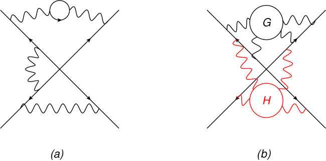
Figure 8: (a) Example diagram generated by the path integral in Eq. (117), with straight semi-infinite Wilson lines for illustration, containing three subdiagrams. (b) Example diagram in the replicated theory, with different colours denoting different replicas.

Now let us generate $N$ independent copies or replicas of the gauge and fermion fields, labelled by $\{A_{\mu}^{(j)}\}$ and $\{\psi^{(j)}\}$, such that particle species with different replica number $j$ never interact. The soft function in such a theory, involving the same $n$ Wilson lines (which are not replicated) is given by

$${\cal S}_{n,R}\,=\,\int{\cal D}A^{(1)}_{\mu}\ldots\int{\cal D}A^{(N)}_{\mu}\exp\left[{\rm i}e\sum_{j=1}^{N}\sum_{i=1}^{n}\int dx_{i}^{\mu}A^{(j)}_{\mu}+\sum_{j=1}^{N}S\left(A_{\mu}^{(j)},\bar{\psi}^{(j)},\psi^{(j)}\right)\right]\,.$$ (118)

Note that the sum in the Wilson line term in Eq. (118) is over both the replica numbers and the external lines, since all replicated gauge fields may interact with any given Wilson line. Furthermore, the fact that the action for the replicated theory is just the sum of the actions of individual replicas follows from the fact that replicas are non-interacting. Carrying out the path integral in the replicated theory amounts to generating Feynman diagrams such as that shown in Fig. 8(b). Any such diagram must be built of connected subdiagrams, such as $G$ and $H$ in the figure, and each individual connected subdiagram must contain only a single replica number, given that the replicated gauge fields only interact with their respective replicated fermions, and with the Wilson lines.

The replicated soft function in Eq. (117) is therefore related to the original soft function simply by

$${\cal S}_{n,R}\,=\,{\cal S}_{n}^{N}\,,$$ (119)

which can be expanded in powers of $N$ to obtain

$${\cal S}_{n,R}\,=\,1+N\log\left({\cal S}_{n}\right)+{\cal O}(N^{2})\,.$$ (120)

It follows that one may write

$${\cal S}_{n}\,=\,\exp\left[\sum_{W}W\right]\,,$$ (121)

where the sum is over diagrams $W$ that are precisely ${\cal O}(N)$ in the replicated theory. To find these, note that mutual independence of the replicated fields implies that a diagram containing $m$ connected subdiagrams must be ${\cal O}(N^{m})$, given that there is a choice of $N$ possible replicas for each subdiagram. Thus, the logarithm of the soft function in QED must contain only connected subdiagrams. This result was originally derived using detailed combinatorial arguments [113], which are rather elegantly circumvented using the replica approach.

In QCD, the combinatorics of exponentiation becomes more complicated due to the non-commuting nature of the emission vertices coupling gluons to the Wilson lines. Nevertheless, the replica trick argument still works [28], and leads to conclude that the logarithm of the soft function, for processes involving only two partons, is built with subdiagrams that are two-line irreducible, which were dubbed webs in the pioneering work of Refs. [9, 10, 11]. Similar methods apply to the case of three partons, but when more than three coloured particles are involved the nature of webs becomes more complicated, due to the multiple possible colour flows contributing to the amplitude. Again, however, the replica trick can be used to reconstruct the logarithm of the soft function [83]. In the multi-parton case, webs turn out to be sets of diagrams related to each other by permutations of gluon attachments to the Wilson lines [83, 84]. Multi-parton webs are governed by interesting mathematical objects known as web mixing matrices, whose combinatorial properties are continuing to be explored [87, 88, 91].

The arguments just discussed apply directly only to the case of virtual contributions to the soft function, which arise from a single vacuum expectation value of Wilson lines. Including also real emissions, we must define the soft function according to Eq. (16), which contains two expectation values involving non-trivial external states, as well as integrals over the multi-gluon phase space. This does not prevent us from using the replica trick: the arguments of this appendix can be used to straightforwardly prove exponentiation at cross-section level, provided real radiations associated with different replica numbers are mutually independent. The latter requirement is fulfilled if the phase space integral for $n$ gluon emissions factorises into $n$ decoupled single-gluon phase space integrals. This condition is satisfied at LL accuracy, as discussed in Section 2.

In this brief summary, we have explicitly discussed only leading-power soft effects, such that the soft function is defined in terms of vacuum expectation values of conventional Wilson lines, as in Eq. (16). The argument, however, readily generalises to the next-to-soft function defined in Eq. (46), which involves the generalised Wilson lines of Eq. (41). Crucial in the definition of Eq. (46) is that the sum over final states involves only leading-power (and therefore uncorrelated) phase space integrals for $n$ gluon emissions. Thus, the replica trick is not invalidated, given that emissions of different gluon replicas remain independent, even at next-to-soft level.

Appendix B Mellin transforms of NLP contributions

In this Appendix, we collect known results concerning the Mellin transforms of logarithmic threshold contributions to hadronic cross sections, both at leading and next-to-leading power. The relevant integrals that need to be performed in order to compute the Sudakov exponent at LP and NLP can be written as

$${\cal D}_{p}(N)=\int_{0}^{1}dz\,\frac{z^{N-1}-1}{1-z}\,\ln^{p}(1-z)\,,\qquad{\cal J}_{p}(N)=\int_{0}^{1}dz\,z^{N-1}\,\ln^{p}(1-z)\,.$$ (122)

These integrals were computed to the required accuracy (that is, up to corrections suppressed by $N^{-2}$ at large $N$) for example in Ref. [36], with the results

$${\cal D}_{p}(N) = \frac{1}{p+1}\,\sum_{k=0}^{p+1}d_{k}(N)\,\binom{p+1}{k}\,(-\ln N)^{p+1-k}+{\cal O}\left(\frac{\ln^{m}N}{N^{2}}\right)\,,$$

$${\cal J}_{p}(N) = \frac{1}{N}\,\sum_{k=0}^{p}\Gamma^{(k)}(1)\,\binom{p}{k}\,(-\ln N)^{p-k}+{\cal O}\left(\frac{\ln^{m}N}{N^{2}}\right)\,,$$ (123)

where $\Gamma^{(k)}$ is the $k$-th derivative of the $\Gamma$ function, while

$$d_{k}(N)\,\equiv\,\frac{d^{k}}{d\lambda^{k}}\left[\Gamma(1+\lambda)\left(1+\frac{\lambda(1-\lambda)}{2N}\right)\right]_{\lambda=0}\,.$$ (124)

Keeping only leading logarithms at both LP and NLP, one finds

$${\cal D}_{p}(N)\,=\,(-1)^{p+1}\left[\,\frac{1}{p+1}\log^{p+1}N-\frac{\log^{p}N}{2N}\,\right]+\ldots\,,$$ (125)

as well as

$${\cal J}_{p}(N)\,=\,\frac{\left(-\log N\right)^{p}}{N}+\ldots\,.$$ (126)

Considering now the application of these results to Eq. (69), we note that the partonic factor for the ($q\bar{q}$)-channel of the resummed Drell-Yan cross-section at LL accuracy, at ${\cal O}(\alpha_{s}^{m})$, and in Mellin space, takes the form

$$\left(\frac{2\alpha_{s}C_{F}}{\pi}\right)^{m}\frac{1}{m!}\left(\log^{2}N+\frac{\log N}{N}\right)^{m}$$ (127)

$$= \left(\frac{2\alpha_{s}C_{F}}{\pi}\right)^{m}\frac{1}{(m-1)!}\left[2\left(\frac{\log^{2m}N}{2m}-\frac{\log^{2m-1}N}{2N}\right)+\frac{2\log^{2m-1}N}{N}\right]\,.$$

In the second line, we have rewritten the result in order to explicitly recognise the leading-logarithmic contributions to the integrals ${\cal D}_{2m-1}$ and ${\cal J}_{2m-1}$, given in Eq. (125) and in Eq. (126), respectively. One finds then

$$\left(\frac{2\alpha_{s}C_{F}}{\pi}\right)^{m}\frac{2}{(m-1)!}\Big{(}{\cal D}_{2m-1}(N)-{\cal J}_{2m-1}(N)\Big{)}\,,$$ (128)

which leads immediately to Eq. (70).

Appendix C Two gluon emission from the generalised Wilson line

In Section 3.1, we defined a next-to-soft function in terms of generalised Wilson lines, which have been introduced and discussed extensively in Refs. [28, 29]. These operators generate effective Feynman rules for the emission of (next-to-)soft gluons from a given hard particle, and the one-gluon emission terms required for describing radiation at ${\cal O}(\alpha_{s})$ are shown in Eq. (41). However, as Refs. [28, 29] make clear, the required Feynman rules also involve effective vertices describing the emission of two gluons from the same point. These are neglected in the analysis of this paper, for reasons discussed in Section 3.1. It is therefore appropriate to check explicitly in a simple example that such vertices cannot contribute to leading-logarithmic NLP terms at higher orders in perturbation theory.

Ignoring coupling and colour factors, the form of the two-gluon emission vertex from a hard scalar particle, in momentum space, is given by [28]

$$R_{\mu\nu}(p;k,l)\propto\frac{(p\cdot k)(p\cdot l)\eta^{\mu\nu}-p^{\nu}l^{\mu}(p\cdot k)-p^{\mu}k^{\nu}(p\cdot l)+(k\cdot l)p^{\mu}p^{\nu}}{(p\cdot k)(p\cdot l)\left[p\cdot(k+l)\right]}\,,$$ (129)

where $p$ is the hard momentum of the emitting particle, and $(k,l)$ are the soft momenta of the emitted gluons. The latter may also be sums of individual gluon momenta, which will not affect the following.

Throughout the paper, we have considered processes with two incoming massless hard partons carrying four-momenta $p_{1}$ and $p_{2}$. Without loss of generality, let us consider the two-gluon emission vertex as occuring on leg $p_{1}$. Then, as we have argued in Section 3.1, leading logarithmic effects can only come from radiation that is maximally (next-to) soft, as well as collinear. This in turn means that either $k$ or $l$ must be proportional to $p_{1}^{\mu}$ or $p_{2}^{\mu}$. From Eq. (129), it is straightforward to show that $R(p;k,l)$ vanishes if $k\propto p$ or if $l\propto p$. Thus, for a non-zero contribution, both $k$ and $l$ must be proportional to $p_{2}$, yielding

$$R^{\mu\nu}(p_{1};p_{2},p_{2})\,=\,\frac{1}{4(p_{1}\cdot p_{2})}\left[\eta^{\mu\nu}-\frac{\left(p_{1}^{\mu}p_{2}^{\nu}+p_{1}^{\nu}p_{2}^{\mu}\right)}{p_{1}\cdot p_{2}}\right]\,.$$ (130)

In a squared matrix element summed over final state gluon polarisations, the Lorentz indices $\mu$ and $\nu$ must ultimately be contracted with one of the external momenta $p_{1}$ or $p_{2}$, or with a further soft momentum. However, the combination in the square brackets in Eq. (130) acts as a projection tensor, that removes the component of any four-momentum that is collinear with $p_{1}$ or $p_{2}$. We have already seen that leading log behaviour can only arise from soft gluon emissions that are maximally (next-to) soft and collinear. We thus find that the two-gluon emission vertex is irrelevant at LL accuracy.

To be more precise, the above discussion relates only to emissions from a scalar particle. In the case of non-zero spin, an extra contribution to the two-gluon emission vertex appears, that involves the spin generator of the emitting particle. There is however an independent line of argument that allows us to discard this contribution, and that indeed could be applied to the first term of Eq. (129): in position space, a four-point vertex for double gluon emission necessarily involves both gluons being emitted from the same point on the emitting Wilson line, and thus involves one less propagator than contributions involving two separate gluon emissions. As a result, such contributions will not contribute a leading logarithm which, as discussed in Section 3.1, requires a maximal number of integrations over normal variables. We therefore conclude, also in the case of spinning hard particles, that the two-gluon next-to-soft emission vertex can be neglected at LL accuracy.

References

- [1] Particle Data Group Collaboration, M. Tanabashi et al., “Review of Particle Physics,” Phys. Rev. D98 (2018), no. 3, 030001.
- [2] T. O. Eynck, E. Laenen, and L. Magnea, “Exponentiation of the Drell-Yan cross section near partonic threshold in the DIS and MS-bar schemes,” JHEP 06 (2003) 057, hep-ph/0305179.
- [3] G. Altarelli, R. K. Ellis, and G. Martinelli, “Large perturbative corrections to the Drell-Yan process in QCD,” Nucl. Phys. B157 (1979) 461.
- [4] G. Parisi, “Summing large perturbative corrections in QCD,” Phys. Lett. B90 (1980) 295.
- [5] G. Curci and M. Greco, “Large Infrared Corrections in QCD Processes,” Phys. Lett. 92B (1980) 175–178.
- [6] G. Sterman, “Summation of large corrections to short distance hadronic cross-sections,” Nucl. Phys. B281 (1987) 310.
- [7] S. Catani and L. Trentadue, “Resummation of the QCD Perturbative Series for Hard Processes,” Nucl. Phys. B327 (1989) 323.
- [8] S. Catani and L. Trentadue, “Comment on qcd exponentiation at large x,” Nucl. Phys. B353 (1991) 183–186.
- [9] J. G. M. Gatheral, “Exponentiation of eikonal cross-sections in nonabelian gauge theories,” Phys. Lett. B133 (1983) 90.
- [10] J. Frenkel and J. C. Taylor, “Nonabelian eikonal exponentiation,” Nucl. Phys. B246 (1984) 231.
- [11] G. Sterman, “Infrared divergences in perturbative QCD,”. in Tallahassee 1981, Proceedings, Perturbative Quantum Chromodynamics, 22-40.
- [12] G. P. Korchemsky and G. Marchesini, “Structure function for large x and renormalization of wilson loop,” Nucl. Phys. B406 (1993) 225–258, hep-ph/9210281.
- [13] G. P. Korchemsky and G. Marchesini, “Resummation of large infrared corrections using Wilson loops,” Phys. Lett. B313 (1993) 433–440.
- [14] S. Forte and G. Ridolfi, “Renormalization group approach to soft gluon resummation,” Nucl. Phys. B650 (2003) 229–270, hep-ph/0209154.
- [15] H. Contopanagos, E. Laenen, and G. Sterman, “Sudakov factorization and resummation,” Nucl. Phys. B484 (1997) 303–330, hep-ph/9604313.
- [16] T. Becher and M. Neubert, “Threshold resummation in momentum space from effective field theory,” Phys. Rev. Lett. 97 (2006) 082001, hep-ph/0605050.
- [17] M. D. Schwartz, “Resummation and NLO matching of event shapes with effective field theory,” Phys.Rev. D77 (2008) 014026, 0709.2709.
- [18] C. W. Bauer, S. P. Fleming, C. Lee, and G. F. Sterman, “Factorization of e+e- Event Shape Distributions with Hadronic Final States in Soft Collinear Effective Theory,” Phys.Rev. D78 (2008) 034027, 0801.4569.
- [19] J.-y. Chiu, A. Fuhrer, R. Kelley, and A. V. Manohar, “Factorization Structure of Gauge Theory Amplitudes and Application to Hard Scattering Processes at the LHC,” Phys.Rev. D80 (2009) 094013, 0909.0012.
- [20] G. Luisoni and S. Marzani, “QCD resummation for hadronic final states,” J. Phys. G42 (2015), no. 10, 103101, 1505.04084.
- [21] T. Becher, A. Broggio, and A. Ferroglia, “Introduction to Soft-Collinear Effective Theory,” Lect. Notes Phys. 896 (2015) pp.1–206, 1410.1892.
- [22] J. Campbell, J. Huston, and F. Krauss, The Black Book of Quantum Chromodynamics. Oxford University Press, 2017.
- [23] M. Kramer, E. Laenen, and M. Spira, “Soft gluon radiation in Higgs boson production at the LHC,” Nucl. Phys. B511 (1998) 523–549, hep-ph/9611272.
- [24] F. Herzog and B. Mistlberger, “The Soft-Virtual Higgs Cross-section at N3LO and the Convergence of the Threshold Expansion,” 1405.5685.
- [25] F. E. Low, “Bremsstrahlung of very low-energy quanta in elementary particle collisions,” Phys. Rev. 110 (1958) 974–977.
- [26] T. H. Burnett and N. M. Kroll, “Extension of the low soft photon theorem,” Phys. Rev. Lett. 20 (1968) 86.
- [27] V. Del Duca, “High-energy bremsstrahlung theorems for soft photons,” Nucl. Phys. B345 (1990) 369–388.
- [28] E. Laenen, G. Stavenga, and C. D. White, “Path integral approach to eikonal and next-to-eikonal exponentiation,” JHEP 0903 (2009) 054, 0811.2067.
- [29] E. Laenen, L. Magnea, G. Stavenga, and C. D. White, “Next-to-eikonal corrections to soft gluon radiation: a diagrammatic approach,” JHEP 1101 (2011) 141, 1010.1860.
- [30] G. Soar, S. Moch, J. Vermaseren, and A. Vogt, “On Higgs-exchange DIS, physical evolution kernels and fourth-order splitting functions at large x,” Nucl.Phys. B832 (2010) 152–227, 0912.0369.
- [31] S. Moch and A. Vogt, “On non-singlet physical evolution kernels and large-x coefficient functions in perturbative QCD,” JHEP 0911 (2009) 099, 0909.2124.
- [32] S. Moch and A. Vogt, “Threshold Resummation of the Structure Function F(L),” JHEP 0904 (2009) 081, 0902.2342.
- [33] D. de Florian, J. Mazzitelli, S. Moch, and A. Vogt, “Approximate N3LO Higgs-boson production cross section using physical-kernel constraints,” JHEP 10 (2014) 176, 1408.6277.
- [34] N. Lo Presti, A. Almasy, and A. Vogt, “Leading large-x logarithms of the quark & gluon contributions to inclusive Higgs-boson and lepton-pair production,” Phys.Lett. B737 (2014) 120–123, 1407.1553.
- [35] R. Akhoury, M. G. Sotiropoulos, and G. Sterman, “An operator expansion for the elastic limit,” Phys. Rev. Lett. 81 (1998) 3819–3822, hep-ph/9807330.
- [36] E. Laenen, L. Magnea, and G. Stavenga, “On next-to-eikonal corrections to threshold resummation for the Drell-Yan and DIS cross sections,” Phys. Lett. B669 (2008) 173–179, 0807.4412.
- [37] G. Grunberg, “Threshold resummation to any order in (1-x),” 0710.5693.
- [38] G. Grunberg and V. Ravindran, “On threshold resummation beyond leading 1-x order,” JHEP 0910 (2009) 055, 0902.2702.
- [39] G. Grunberg, “Large-x structure of physical evolution kernels in Deep Inelastic Scattering,” Phys.Lett. B687 (2010) 405–409, 0911.4471.
- [40] F. Cachazo and A. Strominger, “Evidence for a New Soft Graviton Theorem,” 1404.4091.
- [41] E. Casali, “Soft sub-leading divergences in Yang-Mills amplitudes,” JHEP 08 (2014) 077, 1404.5551.
- [42] S. G. Naculich and H. J. Schnitzer, “Eikonal methods applied to gravitational scattering amplitudes,” JHEP 05 (2011) 087, 1101.1524.
- [43] C. D. White, “Factorization Properties of Soft Graviton Amplitudes,” JHEP 1105 (2011) 060, 1103.2981.
- [44] S. Oxburgh and C. D. White, “BCJ duality and the double copy in the soft limit,” JHEP 02 (2013) 127, 1210.1110.
- [45] R. Akhoury, R. Saotome, and G. Sterman, “Collinear and Soft Divergences in Perturbative Quantum Gravity,” Phys. Rev. D84 (2011) 104040, 1109.0270.
- [46] A. Laddha and A. Sen, “Logarithmic Terms in the Soft Expansion in Four Dimensions,” JHEP 10 (2018) 056, 1804.09193.
- [47] B. Sahoo and A. Sen, “Classical and Quantum Results on Logarithmic Terms in the Soft Theorem in Four Dimensions,” JHEP 02 (2019) 086, 1808.03288.
- [48] R. Saotome and R. Akhoury, “Relationship Between Gravity and Gauge Scattering in the High Energy Limit,” JHEP 01 (2013) 123, 1210.8111.
- [49] R. Akhoury, R. Saotome, and G. Sterman, “High Energy Scattering in Perturbative Quantum Gravity at Next to Leading Power,” 1308.5204.
- [50] S. Melville, S. G. Naculich, H. J. Schnitzer, and C. D. White, “Wilson line approach to gravity in the high energy limit,” Phys. Rev. D89 (2014), no. 2, 025009, 1306.6019.
- [51] A. Luna, S. Melville, S. G. Naculich, and C. D. White, “Next-to-soft corrections to high energy scattering in QCD and gravity,” JHEP 01 (2017) 052, 1611.02172.
- [52] D. Bonocore, E. Laenen, L. Magnea, S. Melville, L. Vernazza, and C. D. White, “A factorization approach to next-to-leading-power threshold logarithms,” JHEP 06 (2015) 008, 1503.05156.
- [53] D. Bonocore, E. Laenen, L. Magnea, L. Vernazza, and C. D. White, “Non-abelian factorisation for next-to-leading-power threshold logarithms,” JHEP 12 (2016) 121, 1610.06842.
- [54] H. Gervais, “Soft Photon Theorem for High Energy Amplitudes in Yukawa and Scalar Theories,” Phys. Rev. D95 (2017), no. 12, 125009, 1704.00806.
- [55] H. Gervais, “Soft Graviton Emission at High and Low Energies in Yukawa and Scalar Theories,” Phys. Rev. D96 (2017), no. 6, 065007, 1706.03453.
- [56] H. Gervais, Soft Radiation Theorems at All Loop Order in Quantum Field Theory. PhD thesis, SUNY, Stony Brook, 2017-08-04.
- [57] A. J. Larkoski, D. Neill, and I. W. Stewart, “Soft Theorems from Effective Field Theory,” JHEP 06 (2015) 077, 1412.3108.
- [58] D. W. Kolodrubetz, I. Moult, and I. W. Stewart, “Building Blocks for Subleading Helicity Operators,” JHEP 05 (2016) 139, 1601.02607.
- [59] I. Moult, L. Rothen, I. W. Stewart, F. J. Tackmann, and H. X. Zhu, “Subleading Power Corrections for N-Jettiness Subtractions,” Phys. Rev. D95 (2017), no. 7, 074023, 1612.00450.
- [60] I. Moult, I. W. Stewart, and G. Vita, “A subleading operator basis and matching for gg → H,” JHEP 07 (2017) 067, 1703.03408.
- [61] I. Feige, D. W. Kolodrubetz, I. Moult, and I. W. Stewart, “A Complete Basis of Helicity Operators for Subleading Factorization,” JHEP 11 (2017) 142, 1703.03411.
- [62] C.-H. Chang, I. W. Stewart, and G. Vita, “A Subleading Power Operator Basis for the Scalar Quark Current,” 1712.04343.
- [63] M. Beneke, F. Campanario, T. Mannel, and B. D. Pecjak, “Power corrections to anti-B —¿ X(u) l anti-nu (X(s) gamma) decay spectra in the ’shape-function’ region,” JHEP 06 (2005) 071, hep-ph/0411395.
- [64] V. Del Duca, E. Laenen, L. Magnea, L. Vernazza, and C. D. White, “Universality of next-to-leading power threshold effects for colourless final states in hadronic collisions,” JHEP 11 (2017) 057, 1706.04018.
- [65] D. Bonocore, E. Laenen, L. Magnea, L. Vernazza, and C. D. White, “The method of regions and next-to-soft corrections in Drell-Yan production,” Phys.Lett. B742 (2015) 375–382, 1410.6406.
- [66] N. Bahjat-Abbas, J. Sinninghe Damsté, L. Vernazza, and C. D. White, “On next-to-leading power threshold corrections in Drell-Yan production at N3LO,” JHEP 10 (2018) 144, 1807.09246.
- [67] R. Boughezal, X. Liu, and F. Petriello, “Power Corrections in the N-jettiness Subtraction Scheme,” JHEP 03 (2017) 160, 1612.02911.
- [68] R. Boughezal, A. Isgrò, and F. Petriello, “Next-to-leading-logarithmic power corrections for -jettiness subtraction in color-singlet production,” Phys. Rev. D97 (2018), no. 7, 076006, 1802.00456.
- [69] I. Moult, L. Rothen, I. W. Stewart, F. J. Tackmann, and H. X. Zhu, “N -jettiness subtractions for at subleading power,” Phys. Rev. D97 (2018), no. 1, 014013, 1710.03227.
- [70] M. A. Ebert, I. Moult, I. W. Stewart, F. J. Tackmann, G. Vita, and H. X. Zhu, “Power Corrections for N-Jettiness Subtractions at ,” JHEP 12 (2018) 084, 1807.10764.
- [71] M. A. Ebert, I. Moult, I. W. Stewart, F. J. Tackmann, G. Vita, and H. X. Zhu, “Subleading power rapidity divergences and power corrections for qT,” JHEP 04 (2019) 123, 1812.08189.
- [72] M. van Beekveld, W. Beenakker, R. Basu, E. Laenen, A. Misra, and P. Motylinski, “Next-to-leading power threshold effects for resummed prompt photon production,” 1905.11771.
- [73] M. van Beekveld, W. Beenakker, E. Laenen, and C. D. White, “Next-to-leading power threshold effects for inclusive and exclusive processes with final state jets,” 1905.08741.
- [74] I. Moult, I. W. Stewart, G. Vita, and H. X. Zhu, “First Subleading Power Resummation for Event Shapes,” JHEP 08 (2018) 013, 1804.04665.
- [75] M. Beneke, A. Broggio, M. Garny, S. Jaskiewicz, R. Szafron, L. Vernazza, and J. Wang, “Leading-logarithmic threshold resummation of the Drell-Yan process at next-to-leading power,” 1809.10631.
- [76] N. Kidonakis and G. Sterman, “Resummation for qcd hard scattering,” Nucl. Phys. B505 (1997) 321–348, hep-ph/9705234.
- [77] A. M. Polyakov, “Gauge Fields as Rings of Glue,” Nucl. Phys. B164 (1980) 171–188.
- [78] I. Ya. Arefeva, “Quantum contour field equations,” Phys. Lett. 93B (1980) 347–353.
- [79] V. S. Dotsenko and S. N. Vergeles, “Renormalizability of Phase Factors in the Nonabelian Gauge Theory,” Nucl. Phys. B169 (1980) 527–546.
- [80] R. A. Brandt, F. Neri, and M.-a. Sato, “Renormalization of Loop Functions for All Loops,” Phys. Rev. D24 (1981) 879.
- [81] G. P. Korchemsky and A. V. Radyushkin, “Loop Space Formalism and Renormalization Group for the Infrared Asymptotics of QCD,” Phys. Lett. B171 (1986) 459–467.
- [82] G. Korchemsky and A. Radyushkin, “Renormalization of the Wilson Loops Beyond the Leading Order,” Nucl. Phys. B283 (1987) 342–364.
- [83] E. Gardi, E. Laenen, G. Stavenga, and C. D. White, “Webs in multiparton scattering using the replica trick,” JHEP 1011 (2010) 155, 1008.0098.
- [84] E. Gardi, J. M. Smillie, and C. D. White, “On the renormalization of multiparton webs,” JHEP 1109 (2011) 114, 1108.1357.
- [85] E. Gardi, J. M. Smillie, and C. D. White, “The Non-Abelian Exponentiation theorem for multiple Wilson lines,” JHEP 1306 (2013) 088, 1304.7040.
- [86] E. Gardi and C. D. White, “General properties of multiparton webs: Proofs from combinatorics,” JHEP 1103 (2011) 079, 1102.0756.
- [87] M. Dukes, E. Gardi, E. Steingrimsson, and C. D. White, “Web worlds, web-colouring matrices, and web-mixing matrices,” J.Comb.Theory Ser. A120 (2013) 1012–1037, 1301.6576.
- [88] M. Dukes, E. Gardi, H. McAslan, D. J. Scott, and C. D. White, “Webs and Posets,” JHEP 1401 (2014) 024, 1310.3127.
- [89] E. Gardi, “From Webs to Polylogarithms,” JHEP 1404 (2014) 044, 1310.5268.
- [90] G. Falcioni, E. Gardi, M. Harley, L. Magnea, and C. D. White, “Multiple Gluon Exchange Webs,” JHEP 1410 (2014) 10, 1407.3477.
- [91] M. Dukes and C. D. White, “Web matrices: structural properties and generating combinatorial identities,” 1603.01589.
- [92] A. Mitov, G. Sterman, and I. Sung, “Diagrammatic Exponentiation for Products of Wilson Lines,” Phys.Rev. D82 (2010) 096010, 1008.0099.
- [93] A. A. Vladimirov, “Exponentiation for products of Wilson lines within the generating function approach,” JHEP 06 (2015) 120, 1501.03316.
- [94] C. D. White, “An Introduction to Webs,” J. Phys. G43 (2016), no. 3, 033002, 1507.02167.
- [95] C. White, “Diagrammatic insights into next-to-soft corrections,” Phys.Lett. B737 (2014) 216–222, 1406.7184.
- [96] M. Beneke, M. Garny, R. Szafron, and J. Wang, “Anomalous dimension of subleading-power N-jet operators,” JHEP 03 (2018) 001, 1712.04416.
- [97] M. Beneke, M. Garny, R. Szafron, and J. Wang, “Anomalous dimension of subleading-power -jet operators. Part II,” JHEP 11 (2018) 112, 1808.04742.
- [98] A. Bhattacharya, I. Moult, I. W. Stewart, and G. Vita, “Helicity Methods for High Multiplicity Subleading Soft and Collinear Limits,” 1812.06950.
- [99] G. F. Sterman, “Partons, factorization and resummation, TASI 95,” in QCD and beyond. Proceedings, Theoretical Advanced Study Institute in Elementary Particle Physics, TASI-95, Boulder, USA, June 4-30, 1995, pp. 327–408. 1995. hep-ph/9606312.
- [100] A. Pak and A. Smirnov, “Geometric approach to asymptotic expansion of Feynman integrals,” Eur.Phys.J. C71 (2011) 1626, 1011.4863.
- [101] B. Jantzen, “Foundation and generalization of the expansion by regions,” JHEP 1112 (2011) 076, 1111.2589.
- [102] B. Jantzen, A. V. Smirnov, and V. A. Smirnov, “Expansion by regions: revealing potential and Glauber regions automatically,” Eur. Phys. J. C72 (2012) 2139, 1206.0546.
- [103] R. K. Ellis, W. J. Stirling, and B. R. Webber, “QCD and collider physics,” Camb. Monogr. Part. Phys. Nucl. Phys. Cosmol. 8 (1996) 1–435.
- [104] S. Moch and A. Vogt, “Higher-order soft corrections to lepton pair and Higgs boson production,” Phys. Lett. B631 (2005) 48–57, hep-ph/0508265.
- [105] E. Laenen and L. Magnea, “Threshold resummation for electroweak annihilation from DIS data,” Phys. Lett. B632 (2006) 270–276, hep-ph/0508284.
- [106] A. Idilbi, X.-d. Ji, J.-P. Ma, and F. Yuan, “Threshold resummation for Higgs production in effective field theory,” Phys. Rev. D73 (2006) 077501, hep-ph/0509294.
- [107] V. Ravindran, “On Sudakov and soft resummations in QCD,” Nucl. Phys. B746 (2006) 58–76, hep-ph/0512249.
- [108] Y. L. Dokshitzer, G. Marchesini, and G. P. Salam, “Revisiting parton evolution and the large-x limit,” Phys. Lett. B634 (2006) 504–507, hep-ph/0511302.
- [109] J. C. Collins, D. E. Soper, and G. F. Sterman, “Factorization for Short Distance Hadron - Hadron Scattering,” Nucl. Phys. B261 (1985) 104–142.
- [110] J. C. Collins, D. E. Soper, and G. F. Sterman, “Soft Gluons and Factorization,” Nucl. Phys. B308 (1988) 833–856.
- [111] I. Z. Rothstein and I. W. Stewart, “An Effective Field Theory for Forward Scattering and Factorization Violation,” JHEP 08 (2016) 025, 1601.04695.
- [112] I. Moult, I. W. Stewart, and G. Vita, “Subleading Power Factorization with Radiative Functions,” 1905.07411.
- [113] D. R. Yennie, S. C. Frautschi, and H. Suura, “The infrared divergence phenomena and high-energy processes,” Ann. Phys. 13 (1961) 379–452.