The Network Effect in Credit Concentration Risk

1.   Introduction

Concentration risk arises in a credit portfolio when there is an uneven distribution of exposures in the portfolio. This occurs in two ways: individual borrowers (single-name concentration) or groups of borrowers aggregated by sectors or geographical regions (sectoral concentration).

Concentrations are important because the theoretical foundations of Basel risk-based capital requirements capital requirements assume infinite granularity of a portfolio. The are based on the Asymptotic Single Risk Factor (ASRF) model, assuming an infinitely large pool of loans resulting in a diversified credit risk portfolio [10]. This assumption enables an analytical solution for capital requirement calculation. Because of this, additional capital is required against this risk [2].

From a micro-prudential perspective, credit concentration has been associated with increased risk of bank failures and increased magnitude of these failures when they occur. Credit concentrations are also important to macro-prudential supervisors when they have the responsibility of identifying and mitigating sources of systemic risk across the financial system. Several banks lending to the same counterparty is an example of system risk arising from credit concentration.

The consequences of not appropriately measuring and mitigating credit concentration risk can be catastrophic. It has been a hallmark of several recent financial crises in Ireland and other OECD economies. Concentrations arise at several layers of disaggregation: first, at a sector level such as property, within that sector at a commercial property level, and then at a key number of large developers within that sector. Lending in this sector is particularly cyclical, and therefore subject to more abrupt declines in collateral values.

In the Irish crisis and the subsequent parliamentary inquiry that followed, one senior executive of an Irish credit institution recounted that the top 30 exposures accounted for over 50% of the bank’s total exposure, and 48% of its profit . That firm was subsequently liquidated. This problem has occurred previously as several banks suffered large losses related to Worldcom, Enron, and Parmalat, as well as the large commercial real estate losses experienced by US banks in the late 1980s [2].

In practice, bank credit portfolios can have concentrated exposures relating to specific obligors or sectors depending on their business models. To capture this specific aspect of credit risk, credit concentration risk is specifically addressed in the Supervisory Review and Evaluation Process (SREP) as a capital surcharge, under Pillar 2. In Pillar 2 capital requirements, concentration risk charges apply to an individual institution. However, individual institutions can have overlapping portfolios of obligors, some of which may be important to individual banks and to the system as a whole. In this paper, we focus on name concentration - typically a feature of Corporate /Commercial Real Estate or other types of specialised lending.

We make three main contributions to existing research. The first one conceptualises credit risk using a system-wide approach based on network science. We integrate two strands of the research literature, credit risk measurement and network science, providing for a metric that measures interdependence due to overlapping portfolios. This approach is general and could be applied to other types of assets, sectors or geographic areas. Second, we demonstrate how this system wide credit concentration risk measure can be practically applied, by providing an analytical estimate of the additional prudential capital that corresponds to this type of credit risk concentration. Third, using simulated and real-world data, we show how this additional capital formula can be calibrated with respect to existing capital requirements and to avoid double counting with the granularity adjustment.

2.   Related work and research contribution

Various proposals exist for calculation of name or sector concentration risk to adjust the ASRF approach. For single-name concentration, existing methods are based on some form of granularity adjustment. These include the Herfindhal-Hirschmann Index or Gini. Depending on the implementation, these measures may not reflect changes in obligor risk [11, 9, 5].

Sector concentration risk can be calculated using multi-factor models taking into account the systematic risk associated with that sector [18], or derive analytical approximations that require simplifying assumptions such as intra-sector correlations remaining constant [13].

Since the 2007 crisis, various types of inter-disciplinary approaches to measuring concentration risk have been developed. The literature merging network theory with various approaches to measuring systemic risk includes work by Alter et al.[1], and Levy-Carciente et al. [14], as well as earlier work by Huang et al.[12] and Caccioli et al.[6]. In their frameworks, similar to ours, they use bipartite networks to describe interconnectedness through various measures. However, the primary purpose of their analysis is to use the asset side of the bank balance sheet as part of mechanism of cascading failures driven by links through the interbank market. This is used to investigate the dynamics of cascading bank failures in response to an initial shock to asset value.

In our approach, we are interested in identifying the aspects of structural systemic risk with a focus on borrowers as the source of risk, rather than the dynamics of a cascading interbank failure. Our work focuses on distinguishing the effect of common exposures across banks, and not within banks. While this network effect is implicitly encapsulated in the works by Huang et al.[12] and Caccioli et al.[6], we wish to make it explicit, and develop a measure that does not require long Monte Carlo simulations and can be used to calculate additional capital requirements specifically related to this type of risk. The paper by Das [8] focusses on measuring systemic risk in a flexible manner with the help of network based properties. However, he does not develop how network metrics interact with the existing regulatory framework. Our work has also some common elements with that by Alter et al.[1], in that we link common exposures to across the system to capital requirements. However, our credit risk mechanism is very different to the Creditmetrics approach used in their work.

We draw on network science, in particular the paper by Zhou et al. [19], to build a projected network from a bipartite network and quantify the impact of lenders onto each others. The work by Zhou et al. has been developed for a different purpose (strategies in recommendation systems), but the logic of their model is also useful in addressing our problem.

3.   Methodology

Based on the existing work and the motivating examples given in the introduction, we have several requirements for a framework that can fully describe interconnectedness due to common exposures. First, the framework should take into account not only the presence of a connection, but its magnitude and risk. Second, it should be tractable enough to decompose individual exposure contributions and their effect overall credit concentration risk within a given system. Third, it should also be able to quantify the effect concentrations within one bank on other banks. Finally, the framework should calculate the effect of changes in risky exposures through changes in the network topology. As the focus is on credit concentration risk, we only consider a simplified subset of a complex system involving lenders and borrowers.

We consider a set of $n$ lenders and $m$ borrowers, with the following simplifications:

1. We assume that lenders and borrowers are two distinct sets (e.g. we neglect interbank loans).

2. We neglect lenders liabilities structures.

These assumptions are reasonable as we want to focus on the structural nature of systemic risk, building on within single institution credit concentration risk.

This problem can be represented as a bipartite network where one layer corresponds to the lenders and the other to their borrowers (Fig. 1).The link between a lender and a borrower represents the exposure of the lender to the debt of the considered borrower.

Figure 1: Representation of a system of $n=3$ lenders and $m=4$ borrowers as a bipartite network.

A common measure of portfolio concentration (e.g. for a bank) is the Herfindhal-Hirschman Index (HHI):

$$HHI=\frac{\sum_{k}E_{k}^{2}}{\left(\sum_{k}E_{k}\right)^{2}},$$ (1)

where the sums are calculated over the borrowers and $E_{k}$ is the exposure of the considered lender to the borrower $k$.

The HHI is a simple metric that can be used to measure the credit concentration risk at the level of each considered institution. However, pairs of lenders may be exposed to the same borrowers, generating further concentration risk on a system wide level. In practice, the HHI does not take into account the potential risk inherent to common exposures.

As mentioned earlier, our problem has similarities with the one investigated by Zhou et al [19]. In our case, we have a bipartite network that comprises two layers: a layer of financial institutions (e.g. banks) and a layer of borrowers. Similarly to the network of users and products, here we wish to quantify the similarities in the composition of financial institutions portfolios. We therefore define a Dependency Index $DI$ based on a modification of the quantity proposed by [19]. Our Dependency Index is defined as the metric in [19] except for the fact that the considered bipartite network of banks and counterparties is weighted, as in [15].

To calculate the Dependency index, we rescale exposures in a way that takes into consideration the risk of the corresponding borrower. Let $e_{ik}$ be the exposure of lender $i$ to the borrower $k$. We define the risk adjusted exposure $w_{ik}$ of lender $i$ to borrower $k$ as

$$w_{ik}=f(r_{k})e_{ik}$$ (2)

where $f(r_{k})$ is a function of $r_{k}$, the estimated risk of entity $k$. This function modifies the unweighted exposure into a weighted exposure based on a risk measure for entity $k$. This risk measure could be a credit rating, and internal credit scale or probability of default (PD), or a market based metric that can rank order credit risk, such as credit spreads. As a result, $w_{ik}$ is a $n\times m$ matrix that connects $n$ lenders with $m$ borrowers.

At this stage, we project the bipartite network onto the lenders’ layer. In other words, we create a single-layer network where a directional link from lender $i$ to lender $j$ represents the size of impact of $i$ to $j$, corresponding to the systemic effect of credit concentration due to common exposures. The adjacency matrix $S=(s_{ij})$ of this projection is calculated as

$$s_{ij}=\sum_{l=1}^{m}\frac{w_{il}w_{jl}}{\sum_{p=1}^{n}w_{pl}\sum_{q=1}^{m}w_{jq}},$$ (3)

where $w_{il}$ is the element of the adjacency matrix of the bipartite network (from lender $i$ to borrower $l$). The sum over $l$ in Equation (3) runs over the $m$ borrowers. As a result, we obtain a $n\times n$ matrix that only depends on the lenders. We name $S$ impact matrix, as it represents the impact that one portfolio has onto another one due to common exposures. More specifically, given two distinct lenders $i$ and $j$, the element matrix $s_{ij}$ represents the impact that lender $i$ has on lender $j$. For example, if the two portfolios have a large overlap, $s_{ij}$ will be higher. On the other hand, the matrix is not necessarily symmetric, i.e. $s_{ij}\neq s_{ji}$, whenever the two lenders have different total exposures. It is easy to see that the impact of a large lender on a small one will be larger than the one of a small lender to a large one. Finally, each element on the diagonal $s_{ii}$ represents a measure of the amount of exposures of lender $i$ that are not connected to other lenders.

We define Dependency Index ($DI_{i}$) of bank $i$ as a measure of the independence of a bank’s portfolio of exposures in relation with the other banks portfolios:

$$DI_{i}=1-\left[\sum_{j=1}^{n}\left(\frac{s_{ji}}{s_{ii}}\right)^{2}\right]^{-1}.$$ (4)

We can also naturally define a Dependency Index for the whole system as a weighted average over $DI_{i}$:

$$DI_{sys}=\frac{\sum_{i=1}^{n}\sum_{k=1}^{m}w_{ik}DI_{i}}{\sum_{i=1}^{n}\sum_{k=1}^{m}w_{ik}}.$$ (5)

One can immediately see that $DI_{i}$ values are comprised in the interval $[0,1]$, and it can be directly compared with the HHI index in (1), or its risk-adjusted version

$$H_{i}=\frac{\sum_{k}w_{ik}^{2}}{\left(\sum_{k}w_{ik}\right)^{2}}.$$ (6)

It can be shown that the asymmetry of the matrix $S$ is strictly related to the heterogeneity of the total size of exposures in different institutions. In particular, we have that $s_{ij}\neq s_{ji}$ if and only if

$$\sum_{q=1}^{m}w_{jq}\neq\sum_{q=1}^{m}w_{iq}.$$ (7)

The two metrics, $H_{i}$ and $DI_{i}$ should be considered as complementary, as they encapsulate two different aspects of risk concentration, namely the concentration within the same portfolio and the concentration due to common exposures, respectively.

In Appendix A we investigate the properties of the Dependency Index to check that it behaves as expected in a few simple model cases.

4.   Data

In this paper, we use several data sets to illustrate our approach.

4.1.   Data Set 1 (DS1)

The Data Set 1 reports a sample of the real estate and corporate portfolios of two banks. The sample covers approximatively 30% of each banks’ portfolio. Exposures are aggregated by group, so each name corresponds to an independent counterparty. The total number of counterparties is 1100, with only 9 of them that are common to both banks. There are four levels of risk, associated with each counterparty, that we label from 1 (the safest) to 4 (the most risky).

4.2.   Data Set 2 (DS2)

The network from Data Set 2 is created out of a set of leveraged loans. We use a set of 2204 loans issued in USD and reported on a given day in the Markit database. The data set reports several information, including the name of the issuer, the total amount issued, and the price on a given day. Using these data, we create a set of overlapping portfolio using an approach that is described in the next Section.

4.3.   Data Set 3 (DS3)

The Data Set 3 reports exposures from 4 banks. The exposures are aggregated by borrower. More specifically, the data set reports: exposures at default (EAD), probability of default (PD), loss given default (LGD). The data set reports two snapshots of the 4 banks in two consecutive years.

5.   Analysis of common exposures

5.1.   Construction of the bipartite network

The first step in constructing the bipartite network of exposures is to identify the risk-adjusted exposures.

In DS1, as we only have a discrete risk classification, we use the following method. First, we create a homogeneous classification of counterparties’ risk by matching the assessments from each bank. Wherever the two classifications of the same counterparty do not match, we choose the highest (riskier) one. In order to calculate the risk weighted exposures as in (2), we consider the weight function:

$$f(r)=a+b\theta(r-r_{0}),$$ (8)

where $a=0.2$, $b=1$ and $r_{0}=1.5$. In practice, we consider two categories of risk ($r=1$ on one hand and $r>1$ on the other), and give to the low risk exposure a 20% weight with respect to the high risk exposures. This mimics typical rules of calculation of risk weighted assets [3].

In DS2, we create a set of five partially overlapping portfolios in the following way. First, we choose the number of lenders (in this paper, we consider 5 lenders) and assume that each of them has a portfolio exclusively from the loans in the data set. We aggregate the loans by issuer, calculating a risk adjusted total amount. As a proxy of risk for each loan, we use the mid close price. More precisely, we divide each amount by the coresponding price and consider that as a risk adjusted exposure (or sum of exposures). Then, we randomly select 15% of the borrowers and assign them exclusively to a randomly chosen lender. This fraction of “isolated borrowers” is chosen randomly, excluding the largest 10% loans in terms of total amount issued. At this point, we assign exposures using the other 85% of issuers. For each issuer, we divide the total amount issued into three parts, and assign each part to three randomly selected lenders. We choose the three amount randomly, with the only condition that each tranche must not be lower than 20% of the total amount issued.

In DS3, it is natural to use the product PD $\cdot$ EAD as risk-adjusted exposures.

5.2.   Concentration metrics

5.2.1 DS1

The impact matrix between $A$ and $B$ is fairly symmetrical:

$$S=\left(\begin{array}[]{cc}0.983&0.019\\ 0.017&0.981\end{array}\right).$$ (9)

Table 1 shows the calculated properties of the two lenders.

Table 1: Properties of lenders of DS1. HHI and DI are the risk-weighted Herfindhal-Hirschman Index and Dependency Index, respectively. Co-exposures and co-weights are the unweighted and weighted fraction of common exposures with respect to the bank’s total exposure, respectively.

Lender	HHI	DI	Co-exposures (%)	Co-weights (%)
A	0.019	0.00031	3.09	3.75
B	0.011	0.00037	3.84	4.62

As the fraction of portfolio overlap is only between 3 and 4%, the impact matrix shows a weakly coupled (most of the weight is on the diagonal) and symmetric behavior. HHI and DI move in opposite directions, as expected: bank A has a slightly more concentrated portfolio, but it is less susceptible to systemic stress, bank B has a less concentrated portfolio, but it is marginally more susceptible to the systemic risk due to common exposures.

We can investigate this further and project the bipartite network on the borrower side (Fig. 2 shows the network of the largest borrowers). In this projection, the weight of the links represents the interconnectedness of two borrowers in the portfolios. This interconnectedness increases with the size of common exposures across different lenders.

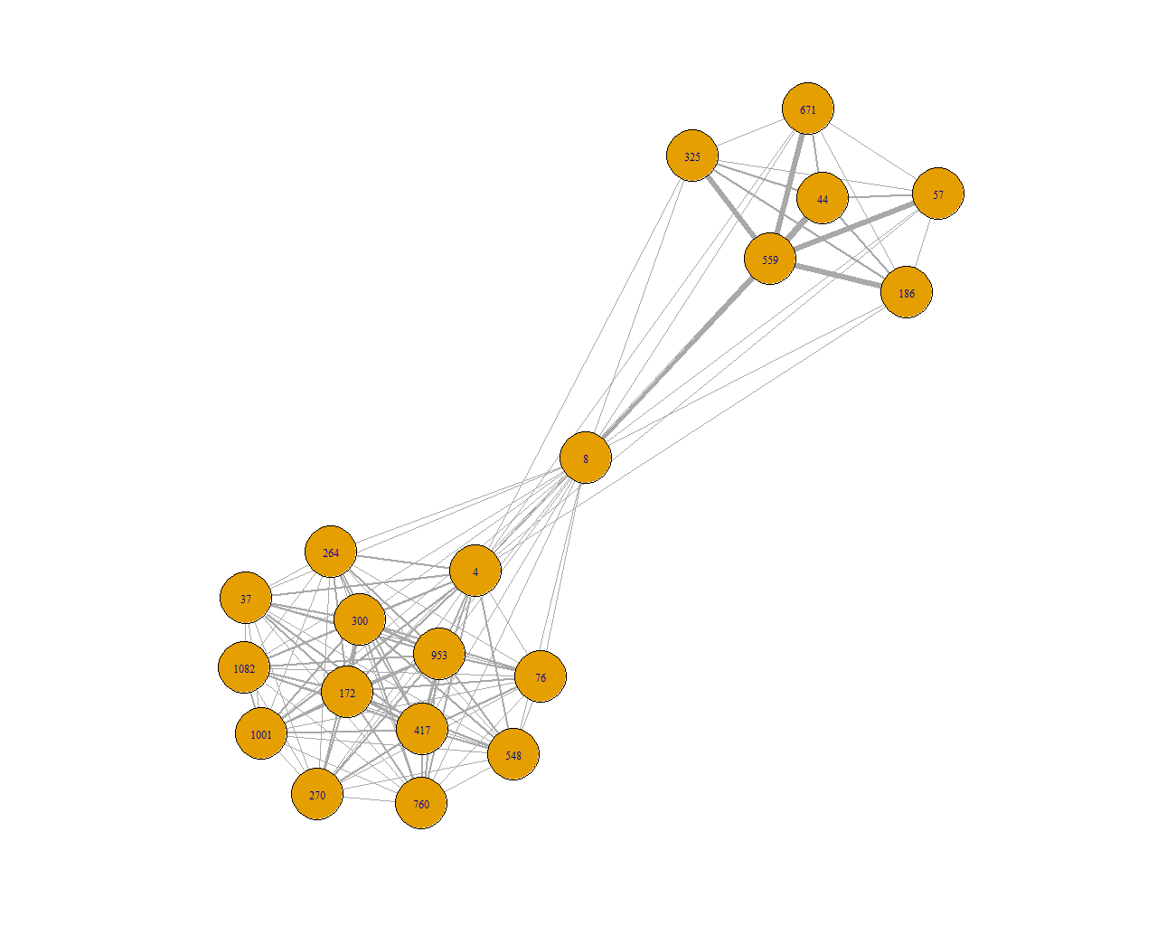
Figure 2: Projected network of interdependencies among the top 20 borrowers of banks A and B in DS1. As the two portfolios have small overlap, it is evident the clustering of the two banks portfolios. As borrowers 4 and 8 are the only ones in the overlap, they have more interconnections across the two groups. Borrowers that are not in the overlap tend to be more strongly connected with the borrowers in the same portfolio.

Fig. 3 displays the composition of the portfolios in terms of risk categories. We can see that while the risk composition of portfolios A and B are fairly similar, the overlap is much more skewed towards higher risk. In particular, we observe that the fraction of exposures in risk category 1 (the safest) are about 9% for bank $A$ and $B$, whereas it is only 3% in the overlap.

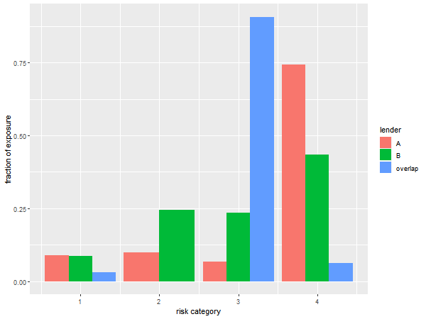
Figure 3: Risk classification of overlapping risk-adjusted exposures in DS1.

5.2.2 DS2

In DS2, we show the impact matrix of the five lenders is:

$$S=\left(\begin{array}[]{ccccc}0.543&0.163&0.214&0.171&0.190\\ 0.073&0.450&0.064&0.135&0.083\\ 0.148&0.098&0.378&0.153&0.202\\ 0.075&0.132&0.097&0.420&0.063\\ 0.160&0.157&0.247&0.121&0.462\\ \end{array}\right).$$ (10)

This synthetic data set has the highest overlap of the three, as it is also shown by the concentration properties in Table 2.

Table 2: Properties of lenders of DS2. HHI and DI are the risk-adjusted Herfindhal-Hirschman Index and Dependency Index, respectively. The co-weights are the risk-adjusted fraction of common exposures with respect to the lenders’ total exposure.

Lender	HHI	DI	Co-weights (%)
A	0.127	0.16585	67.44
B	0.029	0.27937	92.08
C	0.101	0.45663	95.25
D	0.249	0.29145	96.25
E	0.015	0.32574	92.11

In this system, the Dependency Index is much higher than in the other two data sets. This is a combined effect of the high overlap (as in DS3) but also the high granularity of exposures.

5.2.3 DS3

The impact matrix of the four lenders is:

$$S=\left(\begin{array}[]{cccc}0.875&0.147&0.056&0.307\\ 0.079&0.776&0.067&0.269\\ 0.003&0.007&0.863&0.006\\ 0.043&0.070&0.014&0.419\end{array}\right).$$ (11)

As specified earlier, each off-diagonal element of the matrix $s_{ij}$ quantifies the impact of bank $i$ to bank $j$ due to the overlap among the portfolios in the system. So, for example, bank A has a smaller impact on bank C ($s_{13}=0.056$) than on bank D ($s_{14}=0.307$). On the whole, we can see that the interplay of co-exposure impacts is more complex than in DS1. The concentration properties of the four lenders are displayed in Table 3.

Table 3: Properties of lenders of DS3. HHI and D are the risk-adjusted Herfindhal-Hirschman Index and Dependency Index, respectively. Co-exposures and co-weights are the unadjusted and risk-adjusted fraction of common exposures with respect to the lenders’ total exposure, respectively.

Lender	HHI	DI	Co-exposures (%)	Co-weights (%)
A	0.020	0.01046	73.34	75.91
B	0.038	0.04215	83.58	66.13
C	0.336	0.01036	38.22	44.56
D	0.062	0.48734	93.67	97.07

In this data set, there is a sizeable overlap among portfolios, however, this does not always translate into high inter-bank impacts, due to the different sizes of the portfolios involved. For example, the impact of lender A onto lender C is much higher than the impact of lender C to lender A. Another interesting aspect is that sometimes the HHI and DI behave differently. For example, lender D has a comparable HHI to lenders A and B, but a much higher interdependence, whereas lender C has a small Dependency Index due to its low interconnectedness with the rest of the system.

5.3.   Portfolio overlap and risk

The metric of systemic interdependence $DI_{sys}$ also allows us to assess how is distributed the risk across different portfolios. If the overlap between two portfolios were random, the risk distribution of the overlap should be similar to the one of the two portfolios. However, Figure 3 shows that this is not the case. Therefore, we can use the metric $DI_{sys}$ to quantify this difference. In order to do that, we randomly rewire the network and calculate the probability of the scenario observed in the data. We shuffle named counterparties without changing the risk composition of each lender’s portfolio. As a result, the properties that are usually used to measure risk concentration at the lender level do not change. At each randomization, both the HHI and the number of counterparties in the overlap remain the same, and only the link weights within risk categories are permuted. Our metric $DI_{sys}$ of systemic interdependence, though, does change. Fig. 4 shows the distribution of values of $DI_{sys}$ after $N=10^{5}$ randomizations for the data sets DS1 and DS3. In both cases, the probability of observing a value larger than the value of $DI_{sys}$ measured from the data is tiny (it is $0.36\%$ for DS1 and $<0.01\%$ for DS3). This shows that the portfolio overlap among lenders is highly non-random, and skewed towards higher interdependence. The metric of systemic interdependence $DI_{sys}$ allows us to give a quantitative estimation of this phenomenon.

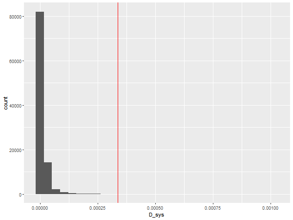
(a) DS1

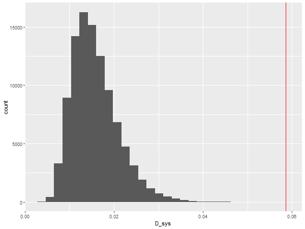
(b) DS3

Figure 4: Distribution of values of $DI_{sys}$ after $N=10^{5}$ randomizations of counterparty names within each risk category. The vertical red bar corresponds to the value calculated from the data.

5.4.   Reaction of the system to increased credit risk

We now test the effect that increasing the risk of counterparties may have on the portfolios interdependence in DS1. First, we imagine a scenario where one of the two low risk (risk category 1) counterparties in the portfolio overlap is downgraded. Table 4 shows that a downgrade of either counterparty (ID 3 and 9) generates an increase of both $DI_{A}$ and $DI_{B}$. We can study the convexity of the Dependency Index by downgrading both counterparties. Table 4 also shows that the simultaneous downgrading of counterparties 3 and 9 generates an increase in $DI_{A}$ and $DI_{B}$ that is about $3.5\%$ higher than the sum of the effect of the two separate downgradings. This shows the effect of the network in amplifying interdependence and systemic risk.

Table 4: Increase of interdependence due to an increase of counterparty risk in DS1. $\Delta DI_{A}$ and $\Delta DI_{B}$ represent the difference in the Dependency Index before and after a downgrading of counterparties in the portfolio overlap.

ID	$\Delta DI_{A}$	$\Delta DI_{B}$
3	$4.7\cdot 10^{-5}$	$5.4\cdot 10^{-5}$
9	$1.9\cdot 10^{-5}$	$2.2\cdot 10^{-5}$
Both	$6.8\cdot 10^{-5}$	$7.9\cdot 10^{-5}$
Difference	$2.4\cdot 10^{-6}$	$2.7\cdot 10^{-6}$
Difference (%)	$3.5\%$	$3.5\%$

5.5.   Sensitivity of the system to an increase in overlapping borrowers

We assess the effect of overlap increase by rewiring isolated exposures into common exposures in DS1. At each iteration, we randomly choose two non-overlapping borrowers, in the same risk class, and merge them, so that they become a common exposure. As in the previous simulations, this rewiring does not change the properties of each portfolio at the bank level, such as the HHI, the risk composition and the total exposure. Fig. 5 shows the effect of overlap increase as measured by $DI_{sys}$. The small non-monotonic jumps are due to the finite number of trials. In fact, it is possible to show that the range of $DI_{sys}$ increases quite rapidly with the increase of overlap.

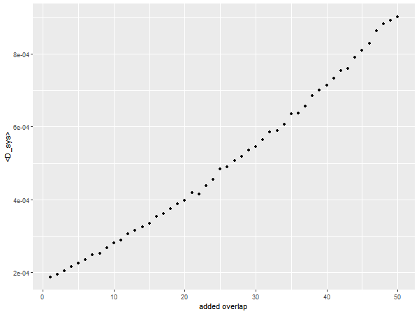
Figure 5: Evolution of $\langle DI_{sys}\rangle$ after increasing the number of overlapping borrowers. The mean is calculated over $N=1000$ iterations.

5.6.   Sensitivity of the system to an increase of borrowers’ risk

A way to characterize the systemic importance of single borrowers is to assess the effect that an increase in their risk may have on global metrics. In order to do that, for each borrower we calculate the difference in $DI_{sys}$ and $HHI_{sys}$ after having increased by a factor 5 all the exposures corresponding to the considered borrower. In this way, we estimate the effect that an increase in its risk has on the concentration parameters of the system. The choice of the factor 5 mimics a typical risk weight prescription of giving 20% of EAD to top tier counterparties and 100% to other counterparties.

Figure 6 shows the result of this test in DS3. We plot the set of points with $\Delta DI_{sys}>0$, corresponding to the borrowers in the overlap. From this scatterplot it transpires that a narrow interval in $\Delta HHI_{sys}$ may correspond to a quite diverse behavior in terms of $\Delta DI_{sys}$. This is another sign of the extra information brought in by the new metric. Besides, the different values of $\Delta DI_{sys}$ provide information on which borrowers are more systemically important whenever their risk should increase. We will use this information to calculate the common exposure add-on in Section 6.

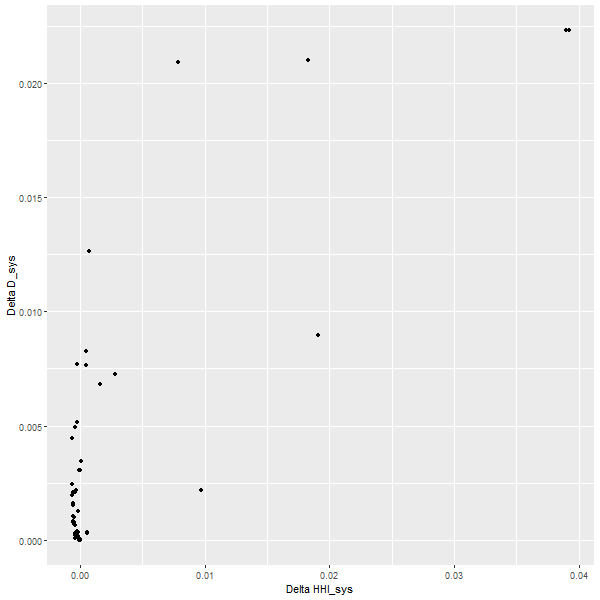
(a) DS3, year 1

(b) DS3, year 2

Figure 6: Sensitivity of the system to an increase in borrowers risk in DS3. Each point represents a borrower whose risk has been increased by multiplying their adjacent exposures by a factor 5.

We have also compared the systemic interdependence sensitivity $\Delta DI_{sys}$ with well known network centrality measures, to verify if the information captured by $\Delta DI_{sys}$ were encapsulated in more common network measures as in [8]. While eigenvector centrality appears to resemble the behavior of $\Delta DI_{sys}$ in one data set, we do not find any conclusive evidence that this holds across all the data sets we consider.

6.   Additional capital requirements of common exposures

The Internal Ratings Based (IRB) capital requirement and the Granularity Adjustment (GA) formula provide an estimation of the capital needed by an institution to be functioning in the occurrence of economic downturns. In Appendix B we give a summary of the relevant formulae of regulatory capital and Granularity adjustment that we are using in this paper. In this section, we wish to calculate a third term, the further additional capital that is required to consider the systemic risk due to common exposures.

6.1.   Common exposure adjustment

Let us consider a lender with a portfolio of $N$ borrowers in a system of lenders with overlapping portfolios. In order to estimate the co-exposure capital add-on, we need a quantity that can give us a measure of the relevance of each borrower in the common exposure risk. As we have seen in Section 5, the increment in the Dependency Index under credit risk increase ($\Delta DI_{i}$) measures exactly that. In analogy with (29), we combine the PD and the Dependency Index and define the corresponding capital requirement as

$$X_{CE}=\sum_{i=1}^{N}s_{i}X_{CE}^{i},$$ (12)

where $s_{i}$ is the fraction of exposures of a given lender to borrower $i$ (i.e. $\sum_{i}s_{i}=1$) and

$$X_{CE}^{i}=MA_{i}\cdot LGD_{i}\left\{\Phi\left[\Phi^{-1}(PD_{i})+\eta\;\Phi^{-1}\left(\frac{1+\theta(\Delta DI_{i})\Delta DI_{i}}{2}\right)\right]-PD_{i}\right\},$$ (13)

where $\theta(x)$ is the step function; in other words, we only consider positive increments of Dependency ($\Delta DI_{i}>0$). When a borrower $i$ is not in the overlap, i.e. only linked to a single institution, its contribution to $X_{CE}$ is zero (note that $\Phi^{-1}(0.5)=0$). This formula depends on the parameter $\eta$, that governs the weight of the systemic co-exposure effect with respect to the other capital requirements.

The measure in (12), however, needs to be calibrated to avoid that part of the risk encapsulated in this term is already considered in the GA term.

6.2.   Example of double counting

Let us consider the particular case represented in Figure 7(a). $(N-1)$ lenders are exposed to $N$ borrowers; each lender has two counterparties; each exposure has the same weight $v$ except the two isolated exposures that have each weight equals to $u$. In order to compare the Dependency Index and the Granularity Adjustment, we define a corresponding system where we aggregate all the lenders into one and sum all the corresponding exposures. The result is shown in Figure 7(b). The common exposures become exposures of the aggregated lender and each has weight $w=2v$, whereas the two isolated exposures remain the same ($u$). As we assume normalized weights, we have $2u+(N-2)w=1$. Due to the homogeneity of common exposures in system (a), we can calculate the GA in system (b) and study its behaviour in terms of the parameters $u$ and $w$. By construction, the parameter $w=2v$ corresponds to the overlap of portfolios in system (a), and the parameter $u$ corresponds to the non overlapping part.

(a) Example of an uniformly co-exposed system of lenders.

(b) Corresponding system where all the lenders have been aggregated into a “superlender” B.

Figure 7: Example of a comparison between a simple system of overlapping portfolios (a) and a corresponding aggregated system (b), with one “superlender” that has the same counterparties and the same aggregated exposures ($w=2v$).

A simple calculation of the Granularity Adjustment $\Gamma$ of system (b) yields:

$$\Gamma=constant\left[1-2(N-2)w+N(N-2)w^{2}\right].$$ (14)

The behaviour of Equation (14) is represented in Figure 8. In this particular example, the behaviour of $\Gamma(w)$ corresponds to the behaviour of the GA as a function of the overlap in system (a). It is easy to see that there are two regimes. When $w>u$, the GA encapsulates the effect of the overlap, because an increase in the overlap and therefore the interdependence of system (a) (i.e. an increase in $w$) corresponds to an increase in the concentration of the portfolio of lender $B$ in system (b). When $w<u$, the GA and the common exposures move in opposite directions, because an increase in the overlap (i.e. an increase in $w$) corresponds to a more homogeneous portfolio for lender $B$. In other words, we can infer that the condition of double counting is

$$\frac{\partial\Gamma}{\partial(overlap)}>0.$$ (15)

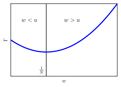
Figure 8: Graphical representation of Equation (14).

6.3.   Derivation of the capital adjustment

We use then this observation and equation (15) to estimate the double counting between the GA and the Dependency Index. Let us distinguish whether the relative exposures $s_{i}$ are in the overlap (i.e. they are shared by at least two lenders) or not, by defining $\Omega$ the set of borrowers in the overlap and $Z$ the set of borrowers not in the overlap, and re-write the Granularity Adjustment (32) as

$$\Gamma=\frac{\sum_{i\in\Omega}s_{i}^{2}\tilde{K}_{i}+\sum_{i\in Z}s_{i}^{2}\tilde{K}_{i}}{\sum_{i\in\Omega}s_{i}{K}_{i}+\sum_{i\in Z}s_{i}{K}_{i}},$$ (16)

where $K_{i}$ is the IRB approach capital corresponding to borrower $i$, and we define

$$\tilde{K}_{i}=\frac{1}{2}C_{i}\left[(\delta-1)K_{i}+R_{i}\right].$$ (17)

Let us know define the weighted means of $K_{i}$ over each subset $\Omega$ and $Z$ as

$$\langle K\rangle_{\Omega}=\frac{\sum_{i\in\Omega}s_{i}{K}_{i}}{\sum_{i\in\Omega}s_{i}}\qquad\langle K\rangle_{Z}=\frac{\sum_{i\in Z}s_{i}{K}_{i}}{\sum_{i\in Z}s_{i}}.$$ (18)

Using these quantities, we can approximate the formula (16) as

$$\Gamma=\frac{\left(\sum_{i\in\Omega}s_{i}^{2}\right)\langle\tilde{K}\rangle_{\Omega}+\left(\sum_{i\in Z}s_{i}^{2}\right)\langle\tilde{K}\rangle_{Z}}{\left(\sum_{i\in\Omega}s_{i}\right)\langle K\rangle_{\Omega}+\left(\sum_{i\in Z}s_{i}\right)\langle K\rangle_{Z}}.$$ (19)

In order to study how the GA behaves with respect to overlap, we assume a small perturbation $\bf{\epsilon}$ of the exposures fractions $\bf{s}$: $\Gamma(\bf{s}^{\prime})=\Gamma(\bf{s+\epsilon})$. The perturbation slightly increases the overlap and decreases the non-overlap by the same amount, more specifically

$$\begin{cases}s_{i}^{\prime}=s_{i}+\epsilon&\mbox{if }i\in\Omega\\ s_{i}^{\prime}=s_{i}-\frac{N_{\Omega}}{N_{Z}}\epsilon&\mbox{if }i\in Z\end{cases}$$ (20)

where $\epsilon>0$, $N_{\Omega}$ is the number of borrowers in the overlap and $N_{Z}=N-N_{\Omega}$ is the number of borrowers outside the overlap. This perturbation increases overlap without changing the total exposures of the considered lender ($\sum_{i}s_{i}=\sum_{i}s_{i}^{\prime}=1$).

After imposing the conditions (20), the overlap in the GA is encapsulated by the scalar parameter $\epsilon$ and we can study how the GA increases with it:

$$\left.\frac{\mbox{d}\Gamma}{\mbox{d}\epsilon}\right|_{\epsilon=0}\geq 0.$$ (21)

Equation (21) is satisfied if and only if

$$r=\frac{N_{\Omega}}{N_{Z}}\frac{2\langle\tilde{K}\rangle_{Z}\sum_{i\in Z}s_{i}\left(\langle K\rangle_{\Omega}\sum_{i\in\Omega}s_{i}+\langle K\rangle_{Z}\sum_{i\in Z}s_{i}\right)+N_{Z}\langle K\rangle_{\Omega}\left(\langle\tilde{K}\rangle_{\Omega}\sum_{i\in\Omega}s_{i}^{2}+\langle\tilde{K}\rangle_{Z}\sum_{i\in Z}s_{i}^{2}\right)}{2\langle\tilde{K}\rangle_{\Omega}\sum_{i\in Z}s_{i}\left(\langle K\rangle_{\Omega}\sum_{i\in\Omega}s_{i}+\langle K\rangle_{Z}\sum_{i\in Z}s_{i}\right)+N_{\Omega}\langle K\rangle_{Z}\left(\langle\tilde{K}\rangle_{\Omega}\sum_{i\in\Omega}s_{i}^{2}+\langle\tilde{K}\rangle_{Z}\sum_{i\in Z}s_{i}^{2}\right)}\leq 1.$$ (22)

Equation (22) gives an estimate on the amount of double counting between the GA and our co-exposure capital $X_{CE}$, to correct the capital adjustment. We propose then a total capital requirement that reads

$$K_{total}=K+\Gamma+K_{CE}(\alpha,\eta),$$ (23)

where the Common Exposure Capital Adjustment $K_{CE}$ is

$$K_{CE}(\alpha,\eta)=[\alpha(r-1)+1]X_{CE}(\eta).$$ (24)

The two parameters ($\alpha$ and $\eta$) govern the capital add-on due to common exposures. The term $[\alpha(r-1)+1]$ in (24) is designed in such a way that when double counting occurs ($r<1$), the co-exposure capital requirement decreases linearly with $r$ (and therefore $K_{CE}<X_{CE}$).

7.   Parameter calibration and application to data

The calibration of parameters $\alpha$ and $\eta$ is obtained by comparison with numerical simulations.

7.1.   Numerical simulations

We perform numerical simulations using as an input the PDs reported in DS3, the data set with the largest overlap. For each lender, we calculate the distribution of losses by uniformly generating random numbers for each borrower $i$ and comparing it with their corresponding $PD_{i}$. In the present work we use $10^{5}$ iterations. We then calculate the Value-at-Risk (VaR) at $q=0.999$ and the expected losses EL. The unexpected losses are simply the difference $UL=VaR-EL$.

We perform these simulations both with the reported data and in a simplified downturn scenario. The downturn scenario is encapsulated by a new set of probabilities of default $PD^{S}$ that we define as

$$PD_{i}^{S}=\sqrt{A\cdot PD_{i}},$$ (25)

where $A=0.3$. We adopt this definition to mimic the effect of a downturn to probabilities of default.

7.2.   Parameter calibration

In order to calibrate the parameters $\alpha$ and $\eta$, we choose a data set and compare the results of the numerical simulations in the downturn scenario with the analytical capital requirements resulting from the sum of the capital calculated in the IRB infinitely granular approach (28) plus the Granularity Adjustment (32). The difference between the analytically calculated capital and the estimation from the numerical simulations constitutes a gap that we use to calibrate the parameters, by setting this gap equal to the common exposure adjustment $K_{CE}$.

This method is not driven by the quite strong assumption that the gap can be entirely explained by the systemic effect of common exposures. Rather, it aims to use the gap as a guide towards a typical scale to which it seems sensible to measure a further capital requirement. In real terms, the systemic effect of common exposures may be larger than what can be captured by Monte Carlo simulations that, differently from the dependency index and analogous network measures, focus on one portfolio at the time.

Table 5 calculates this gap using Data Set 3 (year 1).

Table 5: Calculation of the difference (gap) between the unexpected losses (UL) calculated by Monte Carlo simulations in the adverse scenario described in the text and the analytical calculation of regulatory capital ($K$) plus granularity adjustment ($\Gamma$), using Data Set 3 (year 1).

Lender	UL (numeric)	$K+\Gamma$	Gap
A	0.043	0.036	0.007
B	0.051	0.043	0.008
C	0.232	0.372	-0.139
D	0.074	0.065	0.009

With the exception of lender $C$, the analytically calculated capital requirement ($K+\Gamma$) is smaller than the unexpected losses simulated numerically. In the case of lender $C$, the level of risk of the portfolio appears instead to be completely captured by $K+\Gamma$. Therefore, in the case of lender $C$ we set $K_{CE}=0$. For the other three lenders, instead, we set the gap equal to the co-exposure capital $K_{CE}$ in (24) and use the method of the least squares to fit the parameters. We obtain:

$$\alpha=0.53;\qquad\eta=68.9.$$ (26)

Using the parameters in (26) we can then calculate $K_{CE}$ for the other year of DS3. Table 6 shows the results of this calculation as well as a comparison with the numerical calculation.

Table 6: Calculation of the common exposure capital addition $K_{CE}$ for the system reported in DS3 (year 2).

Lender	UL (numeric)	$K+\Gamma$	$K_{CE}$
A	0.0732	0.0607	0.0136
B	0.0392	0.0339	0.0039
C	0.1312	0.1741	0.0000
D	0.0714	0.0647	0.0045

As we can see, after calibration with a different data set, the capital add-on $K_{CE}$ is able to capture quite well the amount of difference between $K+\Gamma$ and the simulated UL.

8.   Conclusions

In this paper, we propose a new measure of credit concentration risk (Dependency Index) that encapsulates the systemic effect of interconnectedness due to common exposures. We apply this metric on several data sets to illustrate its properties, and we use the metric to calculate analytically the additional capital that quantifies the systemic effect of common exposures risk. The capital add-on can be calibrated to avoid double counting between the granularity adjustment and the co-exposure adjustment.

Broadly speaking, our approach is to measure credit concentration risk at the system level, rather than separately looking at each financial institution portfolios individually. We show that this metric is able to summarize the degree of interdependence in a network of exposures.

The value of the Dependency Index is essentially affected by the network topology and the riskiness of exposures. By testing this metric on a number of data sets, even in the case of low overlap among portfolios, we show that the metric is able to describe the effect of credit risk increase and capture non-linear effects due to the interplay of exposure connectivity. The interdependence analysis also provides insights into the properties of the overlap itself. In particular, we show that the portfolio overlap between two institutions may be highly non-random, and skewed towards higher interdependence. This may be due to a number of reasons: tendency of high risk borrowers to be indebted to multiple institutions, lower credit rating of larger borrowers, etc. Investigating these causal relationships is beyond the scope of the present work, but the Dependency Index allows us to give a quantitative estimation of this phenomenon. We also explore the effect of overlap increase and find that the metric behaves as expected. By comparing the sensitivity of DI and HHI to an increase of borrowers’ risk, we show that the Dependency Index provides extra information on which borrowers are systemically important.

Although approximated, our co-exposure adjustment is able to capture, with only two parameters, an aspect of systemic risk that, to our knowledge, has been neglected so far and the complexity in the interplay among (risk-adjusted) exposures. This is an essential step in developing a more comprehensive methodology to supervise and manage credit risk in a complex system of financial institutions.

Appendix A Properties of the Dependency Index

Metrics of inequality are often tested against a number of properties [7, 16, 17]. Therefore, here we analyse some properties of the Dependency Index $DI$ to check its validity as a measure of co-exposure risk.

A.1.   Minimum Dependency

Dependency $DI_{i}$ of lender $i$ is zero if and only if when lender $i$ has no co-exposures.

We can define this concept more formally as

$$DI_{i}=0\qquad\Leftrightarrow\qquad s_{ji}=0\qquad\textrm{for each}\qquad j\neq i.$$ (27)

This is immediately evident from the definition (4).

A.2.   Transfer to co-exposures

If a lender transfers a fraction of an exposure from an isolated borrower to a co-exposed borrower, by an amount that is small compared with the exposure size, the dependency of that lender increases.

We can see this by focusing on a bipartite network with two lenders ($A$ and $B$), three borrowers (1,2,3) and the following matrix of exposures:

$$W=\left(\begin{array}[]{cc}w_{A1}&0\\ w_{A2}&w_{B2}\\ 0&w_{B3}\end{array}\right).$$

This is the building block of a bipartite network of common exposures (Fig. 9).

Figure 9: Building block of a bipartite network of common exposures.

If we transfer a quantity $\epsilon>0$ from the isolated exposure $1$ to the common exposure $2$ as in

$$\left\{\begin{array}[]{ccc}w^{\prime}_{A1}&=&w_{A1}-\epsilon\\ w^{\prime}_{A2}&=&w_{A2}+\epsilon\end{array}\right.,$$

we can study the effect on the dependency indexes as a function of $\epsilon$. A direct calculation shows that $\partial D_{i}(\epsilon)/\partial\epsilon\geq 0$ for $i=A,B$, so does $DI_{sys}$ by definition.

A.3.   Merging of common exposures (superadditivity)

If two common exposures merge, the dependency metric of the involved lenders increases.

(a) Before the merge

(b) After the merge

Figure 10: Merging of two common exposures. Borrowers 1 and 2 merge and become borrower 3, with $w_{A3}=w_{A1}+w_{A2}$, $w_{B3}=w_{B1}+w_{B2}$.

Let us consider the simplified case of a network with two lenders and two common exposures (Fig. 10(a)), described by the weight matrix:

$$W=\left(\begin{array}[]{cc}w_{A1}&w_{B1}\\ w_{A2}&w_{B2}\end{array}\right).$$

We wish to study the difference in the dependency metrics with the corresponding network characterized by a merging of the two borowers, i.e.

$$W^{\prime}=\left(\begin{array}[]{cc}w_{A3}&w_{B3}\end{array}\right),$$

where $w_{A3}=w_{A1}+w_{A2}$, $w_{B3}=w_{B1}+w_{B2}$ (Fig. 10(b)).

A direct calculation shows that we have always $D^{\prime}_{A}\geq D_{A}$ and $D^{\prime}_{B}\geq D_{B}$. In particular, we have $D^{\prime}_{A}=D_{A}$ and $D^{\prime}_{B}=D_{B}$ if and only if $w_{A1}/w_{A2}=w_{B1}/w_{B2}$, i.e. the merging of two common exposures typically increases the systemic interdependence. The exception is a particular case when the relative exposure of the two lenders to the two borrowers is exactly the same.

A.4.   Effect of isolated exposures

If a lender transfers a fraction of an exposure to a new counterparty that has not borrowed from other lenders, by an amount that is small compared with the exposure size, the Dependency Index of the system decreases.

To see that, we can use the same setting as in Section A.2, where $w_{A1}=0$ and we consider the transfer

$$\left\{\begin{array}[]{ccl}w^{\prime}_{A1}&=&\epsilon\\ w^{\prime}_{A2}&=&w_{A2}-\epsilon\end{array}\right.,$$

where $\epsilon>0$. A direct calculation shows that $D^{\prime}_{A}\leq D_{A}$, $D^{\prime}_{B}\leq D_{B}$, and therefore $D^{\prime}_{sys}\leq DI_{sys}$ by definition.

Appendix B IRB approach and Granularity Adjustment

Let us summarize here the Internal Ratings Based (IRB) approach and the formula of Granularity Adjustment that we use in the paper. Our starting point is recalling the formula of capital calculation according to the IRB approach Basel methodology [4]:

$$K=\sum_{i=1}^{N}s_{i}K_{i},$$ (28)

where the sum runs over all the exposures of the considered lender, $s_{i}$ is the fraction of exposure to borrower $i$, and $K_{i}$ is defined as

$$K_{i}=MA_{i}\left\{LGD_{i}\cdot\Phi\left[\frac{\Phi^{-1}(PD_{i})+\sqrt{\rho_{i}}\Phi^{-1}(q)}{\sqrt{1-\rho_{i}}}\right]-LGD_{i}\cdot PD_{i}\right\},$$ (29)

where $\Phi(x)$ is the cumulative normal distribution and $\Phi^{-1}(x)$ its inverse, $q$ is the $q^{th}$ chosen percentile of the (normally distributed) systematic risk factor, $\rho_{i}$ is the correlation between the returns of borrower $i$ and the systematic risk factor, and $MA_{i}$ is the maturity adjustment, that is estimated as

$$MA_{i}=\frac{1+(M-2.5)b(PD_{i})}{1-1.5b(PD_{i})},$$ (30)

where

$$b(PD)=\left[0.119-0.0548\log(PD)\right].$$ (31)

Typically, one sets $q=0.999$.

As it is well-known, the Basel formula (28) is written for a portfolio that is infinitely granular. It is then necessary to add a Granularity Adjustment (GA). Here we use the Granularity Adjustment proposed by [11]:

$$\Gamma=\frac{1}{2K}\sum_{i=1}^{N}s_{i}^{2}C_{i}\left[\delta(K_{i}+R_{i})-K_{i}\right],$$ (32)

where $R_{i}$ is the loan-loss reserve

$$R_{i}=E[LGD_{i}]\cdot PD_{i},$$ (33)

$\delta$ is a regulatory parameter that is calibrated as $\delta=4.83$ and $C_{i}$ is defined as

$$C_{i}=\frac{\gamma E[LGD_{i}](1-E[LGD_{i}])+E[LGD_{i}]^{2}}{E[LGD_{i}]},$$ (34)

where $\gamma=0.25$ [11].

References

- Adrian Alter and Raupach [2015] Adrian Alter, B. R. C., Raupach, P., May 2015. Centrality-based capital allocations. International Journal of Central Banking, 1–49.
-
Bank of International Settlements [2006]
Bank of International Settlements, 2006. Studies in credit concentration
risk. Bank for International Settlements.
URL {https://www.bis.org/publ/bcbs_wp15.pdf} -
Bank of International Settlements [2015]
Bank of International Settlements, 2015. Revisions to the standardised
approach for credit risk. Bank for International Settlements.
URL https://www.bis.org/bcbs/publ/d347.pdf -
Bank of International Settlements [2017]
Bank of International Settlements, 2017. Basel iii: Finalising post-crisis
reforms. Bank for International Settlements.
URL https://www.bis.org/bcbs/publ/d424.pdf -
Cabedo Semper and Tirado Beltrán [2011]
Cabedo Semper, J. D., Tirado Beltrán, J. M., Oct. 2011. Sector
concentration risk: A model for estimating capital requirements. Mathematical
and Computer Modelling 54 (7-8), 1765–1772.
URL http://dx.doi.org/10.1016/j.mcm.2010.11.086 - Caccioli et al. [2014] Caccioli, F., Shrestha, M., Moore, C., Farmer, J. D., Sep. 2014. Stability analysis of financial contagion due to overlapping portfolios. Journal of Banking and Finance 46 (C), 233–245.
- Calabrese et al. [2012] Calabrese, R., Porro, F., et al., 2012. Single-name concentration risk in credit portfolios: a comparison of concentration indices. University College Dublin, Geary Institute, Discussion Paper Series, WP2012/14.
- Das [2016] Das, S. R., Mar. 2016. Matrix Metrics: Network-Based Systemic Risk Scoring. The Journal of Alternative Investments 18 (4), 33–51.
-
Düllmann and Masschelein [2007]
Düllmann, K., Masschelein, N., Oct. 2007. A tractable model to measure
sector concentration risk in credit portfolios. Journal of Financial Services
Research 32 (1-2), 55–79.
URL http://dx.doi.org/10.1007/s10693-007-0014-3 -
Gordy [2003]
Gordy, M. B., Jul. 2003. A risk-factor model foundation for ratings-based bank
capital rules. Journal of Financial Intermediation 12 (3), 199–232.
URL http://dx.doi.org/10.1016/s1042-9573(03)00040-8 -
Gordy and Lütkebohmert [2013]
Gordy, M. B., Lütkebohmert, E., 2013. Granularity adjustment for regulatory
capital assessment. International Journal of Central Banking 9, 33–70.
URL http://www.ijcb.org/journal/ijcb13q3a2.htm - Huang et al. [2013] Huang, X., Vodenska, I., Havlin, S., Stanley, H. E., Feb. 2013. Cascading Failures in Bi-partite Graphs: Model for Systemic Risk Propagation. Nature Publishing Group 3 (1), 440442–9.
- Kurtz et al. [2018] Kurtz, C., Lütkebohmert, E., Sester, J., 2018. Calculating capital charges for sector concentration risk. Journal of Credit Risk, Forthcoming.
- Levy-Carciente et al. [2015] Levy-Carciente, S., Kenett, D. Y., Avakian, A., Stanley, H. E., Havlin, S., Oct. 2015. Dynamical macroprudential stress testing using network theory. Journal of Banking and Finance 59 (C), 164–181.
-
Liu et al. [2009]
Liu, J., Shang, M., Chen, D., 2009. Personal recommendation based on weighted
bipartite networks. In: 2009 Sixth International Conference on Fuzzy Systems
and Knowledge Discovery. IEEE, pp. 134–137.
URL http://dx.doi.org/10.1109/fskd.2009.469 - Lorenz [1905] Lorenz, M. O., 1905. Methods of measuring the concentration of wealth. Publications of the American statistical association 9 (70), 209–219.
- Lütkebohmert [2008] Lütkebohmert, E., 2008. Concentration risk in credit portfolios. Springer Science & Business Media.
-
Pykhtin [2004]
Pykhtin, M., 2004. Portfolio credit risk multi-factor adjustment.
RISK-LONDON-RISK MAGAZINE LIMITED- 17 (3), 85–90.
URL https://www.risk.net/risk-management/credit-risk/1530333/multi-factor-adjustment - Zhou et al. [2007] Zhou, T., Ren, J., Medo, M., Zhang, Y.-C., Oct. 2007. Bipartite network projection and personal recommendation. Physical Review E 76 (4), 720–7.