Suzaku observation of Jupiter’s X-rays around solar maximum

Abstract

We report on results of imaging and spectral studies of X-ray emission from Jupiter observed by Suzaku. In 2006 Suzaku had found diffuse X-ray emission in 1–5 keV associated with Jovian inner radiation belts. It has been suggested that the emission is caused by the inverse-Compton scattering by ultra-relativistic electrons ($\sim 50$ MeV) in Jupiter’s magnetosphere. To confirm the existence of this emission and to understand its relation to the solar activity, we conducted an additional Suzaku observation in 2014 around the maximum of the 24th solar cycle. As a result, we successfully found again the diffuse emission around Jupiter in 1–5 keV and also point-like emission in 0.4–1 keV. The luminosity of the point-like emission which was probably composed of solar X-ray scattering, charge exchange, or auroral bremsstrahlung emission increased by a factor of $\sim 5$ with respect to 2006, most likely due to an increase of the solar activity. The diffuse emission spectrum in the 1–5 keV band was well-fitted with a flat power-law function ($\Gamma=1.4\pm 0.1$) as in the past observation, which supported the inverse-Compton scattering hypothesis. However, its spatial distribution changed from $\sim 12\times 4$ Jovian radius (Rj) to $\sim 20\times 7$ Rj. The luminosity of the diffuse emission increased by a smaller factor of $\sim 3$. This indicates that the diffuse emission is not simply responding to the solar activity, which is also known to cause little effect on the distribution of high-energy electrons around Jupiter. Further sensitive study of the spatial and spectral distributions of the diffuse hard X-ray emission is important to understand how high-energy particles are accelerated in Jupiter’s magnetosphere.

1 Introduction

X-ray observatories have discovered X-ray emission from several objects in our solar system (Bhardwaj et al., 2007). A study about objects like planets, moons and comets was made feasible for the first time thanks to an advance of performances of the observatories. The X-ray observations of the solar system objects showed their active features and their relation to the solar activity, which will consequently lead us to understand universal relation between stars and planets, by combining with knowledges from other remote or in-situ measurements about them. It has been established that there are three types of the mechanisms of X-ray emission from the objects in the solar system: solar X-ray scattering on the surface or in the atmosphere of the objects, charge exchange (CX) reactions caused by collisions between solar wind containing multivalent ions and a planetary atmosphere containing neutral atoms (Cravens, 2003), and non-thermal emission caused by the acceleration of high energy particles.

Jupiter is the largest and the most luminous planet in our solar system in the X-ray band (Metzger et al., 1983; Waite et al., 1997). Recent X-ray observatories such as Chandra, XMM-Newton, and Suzaku have detected X-ray emission from Jupiter. As results of the Chandra and XMM-Newton observations, Gladstone et al. (2002), Branduardi-Raymont et al. (2004), Elsner et al. (2005), Branduardi-Raymont et al. (2007a), and Branduardi-Raymont et al. (2007b) described that the solar X-ray scattering occurred dominantly on Jupiter’s disk, whereas, in Jupiter’s auroral region, CX emission was caused by heavy ions originated in the solar wind or Jupiter’s magnetosphere such as Io’s plasma source, and non-thermal bremsstrahlung emission was caused by energetic electrons in Jupiter’s magnetosphere. The auroral emission is known to be somewhat solar-driven. Although the majority of the emitting ions/electrons are provided from Jupiter’s moons in the magnetosphere, some originate from the solar wind. The solar wind plasma is strongly accelerated in the Jovian magnetosphere (see e.g. Bunce et al. (2004)).

Ezoe et al. (2010) have discovered diffuse hard X-ray emission, from Suzaku observation in 2006, around Jupiter with a size of $12\times 4$ Jovian radius (Rj) spatially associated with its radiation belts and Io plasma torus. It was world-first and had not been observed by Chandra and XMM-Newton, since Suzaku has a comparative advantage in its sensitivity for such extended emission. They hypothetically considered that the emission was caused by the inverse-Compton scattering by which high energetic electrons ($\sim 50$ MeV) in Jupiter’s magnetosphere energized solar visible photons into the X-ray band. However, they also mentioned that there was a factor of 7–50 discrepancy between the $\sim 50$ MeV electron number density required to explain the X-ray intensity of the diffuse emission and that estimated from the Divine-Garrett empirical charged particle model (Divine & Garret, 1983) based on the data taken with Pioneer and Voyager. Also, so far there has been no knowledge about a relation between the detection of the diffuse emission and the solar activity.

The Jovian diffuse hard X-ray emission has several remaining issues. Hence, to confirm about a reproducibility of the detection of the diffuse emission, we conducted an additional Suzaku observation of Jupiter in 2014 when the solar activity reached around its maximum of the 24th solar cycle. In this paper, we report the results and the relation to the solar activity by comparing with the results of the past observation in 2006 when the solar activity was lowering into its minimum.

2 Observations

Suzaku (Mitsuda et al., 2007) observed Jupiter on 15–21 April 2014 with the X-ray Imaging Spectrometer (XIS: Koyama et al. (2007)). The XIS consists of two front-illuminated (FI) CCDs of XIS0 and XIS3, and one back-illuminated (BI) CCD of XIS1. The particle background of XIS is 2–5 times lower by comparing with the instruments onboard Chandra and XMM-Newton as shown in figure 5 of Mitsuda et al. (2007) which summarizes the background normalized by the effective area and the field of view. This indicates that XIS has good sensitivity determined by background for spatially extended emission.

Jupiter’s motion on the sky ($\sim 20$ arcsec/h in April 2014) required fourteen pointing trims of the spacecraft attitude during the long observations so that the target would not move out of the central region of CCD. The XIS was operated in the normal mode. The data reduction was performed on the nominal final version 3.0.22.44 screened data provided by the Suzaku processing facility by using the HEAsoft analysis package version 6.22.1. The total exposure of each XIS FI and BI chip was $\sim$160 ks. For spectral fits, response matrices and auxiliary files were generated with xisrmfgen and xissimarfgen. We treated the optical loading as a negligible problem (see section 2 in Ezoe et al. (2010)).

The solar activity was going toward its maximum during the observations. In contrast, we were at low activity period just before solar minimum during the past Suzaku observations on 24–28 February 2006. Therefore, we are able to look into the relation between the solar activity and Jupiter’s X-rays by comparing these two observations. We also note that we assumed a distance from Earth to Jupiter as 5.4 AU in the 2014 observations, whereas, the past one had been 5.0 AU. Jupiter rose/set after and before Sun in 2014 and 2006, respectively. The Sun–Jupiter–Earth angle in 2014 was similar to the past observations, $\sim 10^{\circ}$. We need to subtract diffuse background radiations, which are the Soft X-ray Diffuse Background (SXDB) and the Cosmic X-ray Background. The SXDB consists of Galactic emission from Local Hot Bubble and Milky Way Halo, and CXB is the superposition of point sources from distant Active Galactic Nuclei with a rather hard spectrum. They contaminate Jupiter’s X-ray data due to the wide point spread function of Suzaku. By employing events accumulated in outer regions of the XIS field as the background, the above diffuse radiations were subtracted in the spectral data. We, however, decided to omit events below 0.4 keV in the following analyses for the 2014 observations, because Jupiter passed a region where the SXDB is relatively high according to the ROSAT All Sky Survey.

3 Results

3.1 Imaging analysis

Since Jupiter was moving in the field of view, we had to correct for the motion and convert the data coordinates into Jupiter’s reference system to detect emission from Jupiter. We used Jupiter’s ephemeris obtained from the Jet Propulsion Laboratory (JPL). At first, before the above-mentioned procedure, we examined X-ray images without the attitude correction. Figure 1 shows mosaic images of BI and FI CCDs in two bands of 0.4–1 and 1–5 keV, respectively. The images were divided by exposure maps which were generated by the exposure map generator xisexpmapgen. Both of the images, especially the 0.4–1 keV one, show faint trails along Jupiter’s motion as an evidence of a detection of Jupiter’s X-rays.

There are signatures of emission from point sources in the background beside Jupiter’s trail. In particular, it is noticeable in the 1–5 keV image. Therefore, we utilized the 1–5 keV image, checked it against the celestial catalogue of XMM-Newton Serendipitous Source Catalog (3XMM-DR8 version), used wavdetect which is a point search program in the CIAO package, and identified a total of forty four point sources. The obtained point source positions are shown in figure 1 as green circles with a red slash. We excluded the circular regions centered at individual sources. The diameter is equal to the beam size or the half power diameter (HPD) of XIS ($\sim 2$ arcmin). For safety, we decided to remove X-ray photons from these forty four point sources in both analyses of the 0.4–1 and 1–5 keV images.

We corrected the two band images for Jupiter’s motion and created Jupiter’s reference frame images. For both images in the 0.4–1 and 1–5 keV bands, we created exposure maps for every 2048 s interval, corresponding to 256 XIS default time bins (8 s each). Jupiter’s migration length in the 2048 s interval was $\sim 10$ arcsec as estimated from Jupiter’s apparent velocity, causing a very small image blur compared with the Suzaku’s HPD ($\sim 2$ arcmin). We also excluded the forty four point source regions from every exposure map. We subsequently corrected the coordinates of all the chopped exposure maps by considering Jupiter’s motion and reconstructed them into one exposure map for every CCD. We finally divided the X-ray image by the reconstructed exposure map in Jupiter’s reference frame.

Figure 2 shows the obtained images. We detected that hard X-ray emission significantly extended over $\sim$20 $\times$ 7 Rj which is larger than the result of the 2006 Suzaku observation associated with Jovian radiation belts and Io’s orbit (see figure 2 in Ezoe et al. (2010)). Figure 2 shows that Jupiter’s soft X-rays likely correspond to a point-spread function of Suzaku, in contrast, the hard X-rays are surely more extended than it. To examine the distribution of the emission quantitatively, we produced projection profiles along the horizontal axis as shown in figure 3. We simulated emission distributions from Jupiter’s body (disk and aurorae) and from its surroundings by presuming their shapes to be a small circle and an ellipse, respectively. We found that the profile can be roughly represented by a simulated model using xissimarfgen, which consists of a uniform circular emission with Jovian radius of 18.3 arcsec and a uniform elliptical emission with semi-axes of 6 and 2 arcmin (20 and 7 Rj). The hard emission is surely extended over a wide region ($>6$ Rj). On the other hand, the soft emission was marginally consistent with the small circular emission from Jupiter’s body.

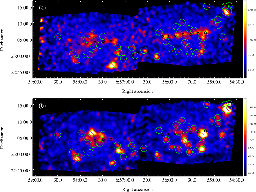
Figure 1: Suzaku XIS mosaic images of the vicinity of Jupiter in the (a) 0.4–1 keV (BI) and (b) 1–5 keV (FI) bands, displayed on the J2000.0 coordinates. Exposures are corrected and the count unit is counts s^-1 binned pixel^-1. For clarity, the images are binned by a factor of 8 and smoothed by a Gaussian of $\sigma$ $=$ 5 pixels. Black circles show the size and pass of Jupiter during the observations. Green circles with a red slash mark omitted point source regions when we create the images in Jupiter reference frame coordinates and the spectra (see the text).

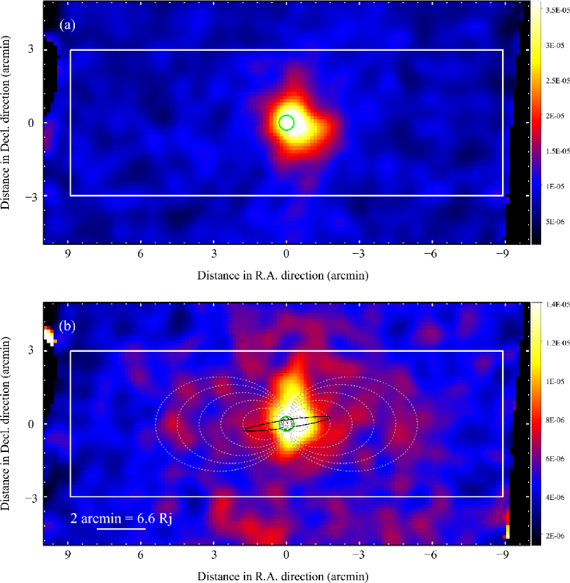
Figure 2: Suzaku XIS images after correcting for Jupiter’s ephemeris in the (a) 0.4–1 keV (BI) and (b) 1–5 keV (FI) bands. The images are binned and smoothed in the same way as figure 1. In panel (a) and (b), a green circle indicates the expected position and size of Jupiter with Jovian radius of18.3 arcsec. In panel (b), gray dashed-lines indicate the magnetic field lines at 3, 6, 9, 12, 15, and 18 Jovian radius (Rj). A black line is the path traced by Io. A schematic diagram of Jupiter was generated by Jupiter Viewer Tool, PDS Rings Node. White boxes show the regions used to obtain projection profiles in figure 3.

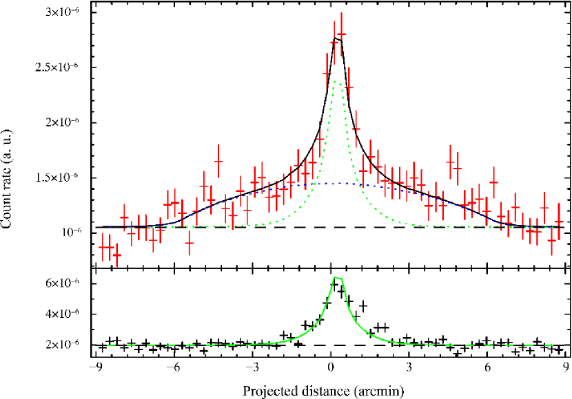
Figure 3: Projection profiles along the horizontal axis, extracted from box regions in figure 2. Black and red crosses show the 0.4–1 and 1–5 keV data, respectively. Errors are 1$\sigma$ statistical ones. Green lines indicate a simplified model of X-rays from Jupiter’s body (18.3 arcsec radius) in 0.4–1 keV (solid line) and 1–5 keV (dotted line). A dotted blue line indicates an expected profile of a uniform emission extended over an elliptical region with semi-axes of 6 and 2 arcmin. A solid black line is the sum of the dotted green and blue lines. Dashed black lines are background levels. The normalizations and offsets of these lines are tuned by fitting to the data.

3.2 Spectral analysis

In order to investigate the characteristics of Jupiter’s X-ray emission, we analyzed the spectrum by extracting photons from the extended emission region. We excluded the above-mentioned forty four point sources in the background from each of the event files at first. In the same way as in generating the exposure maps, we partitioned the original event file into several parts of 2048 s duration, and then extracted source photons from a circle with a radius of 6 arcmin and background ones from the surrounding annulus with an outer radius of 8 arcmin. Both regions are centered on the path of Jupiter at any time. Consequently, the source region includes both Jupiter’s body and diffuse emission because of the limitation of Suzaku’s angular resolution (HPD of $\sim 2$ arcmin) which hampers us to separate them spatially. In the following spectral fits, we used XSPEC version 12.9.0. The diffuse background component was subtracted using the background photons in the outer annular region. The apparent size of Jupiter’s body is small against the source region, and we may ignore that Jupiter occults a part of the diffuse background radiation.

The spectrum thus obtained is shown in figure 4. It seems to show several lines, with a thermal plasma continuum in the lower energy side and a continuum extending up to $>5$ keV. We firstly tried to fit a model consisting of five Gaussians combined with an APEC model and a power-law function to the spectra. We included no absorbing column in the model, as expected from the proximity of the source object. The five Gaussians had fixed line energies: 0.57, 0.65, 0.82, 1.02, and 1.35 keV which are the known values of O VII, O VIII Ly$\alpha$, Fe XVIII, Ne X, and Mg XI lines, respectively. We assumed that O VII and O VIII Ly$\alpha$ lines are CX emission from Jupiter’s aurorae, whereas Fe XVIII, Ne X, and Mg XI lines are scattered solar coronal emission from Jupiter’s disk. The first fit to the data gave $\chi^{2}/\nu$ of $\sim$ 1.12. However, we found a difference around 0.5 keV between the model and the spectra. Therefore, we next allowed the line energy of the first gaussian at 0.57 keV to be free and fitted again to the same spectrum. This second fitted model represented the data better than the first one with $\chi^{2}/\nu$ of $\sim$ 0.70. We employed this second model as the best-fit model because of the $\chi^{2}/\nu$ value. Table 3.2 lists the best fit parameters and 90% confidence errors. The obtained $\Gamma$ of the power-law function is $1.4\pm 0.1$, consistent with the spectra obtained in the 2006 Suzaku observation. This quite flat power-law is thought to be corresponding to the non-thermal emission discovered from the past Suzaku observation.

The line energy of the first Gaussian in the best-fit model is 0.53 keV, which does not correspond to any likely value caused by the CX reaction. It is supposedly considered that the emission in this region is a line complex of oxygen and nitrogen ions. Then, we finally tried to fit with six Gaussians by adding one Gaussian, whose line energy was fixed at 0.50 keV to represent the N VII line, to the first model. This third model fitted the spectrum as well as the first one with $\chi^{2}/\nu$ of $\sim 0.92$, but showed a slight remaining discrepancy around 0.5 keV.

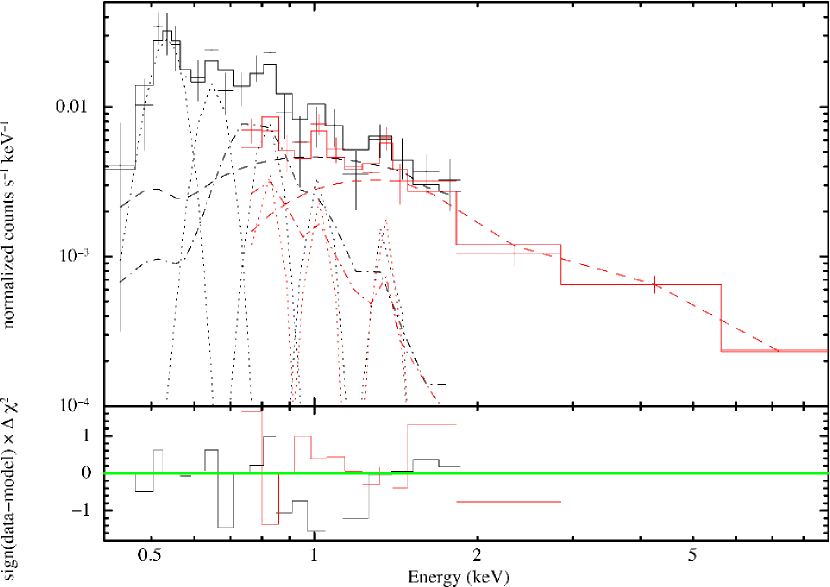
Figure 4: Background subtracted BI (black) and FI (red) spectra of the extended emission region, compared with the best-fit models summarized in table 3.2 (solid lines). APEC model, a power-law function, and Gaussians are shown in dash-dotted, dashed, and dotted lines, respectively. Energies of the Gaussian lines (dotted curves) are 0.53$\pm$0.01, 0.65, 0.82, 1.02, and 1.35 keV, representing a possible N VII and O VII mixture, O VIII Ly$\alpha$, Fe XVIII, Ne X, and Mg XI lines, respectively. The line energies of the latter four lines are fixed in the spectral fits.

Best co-fit parameters (and their 90% confidence errors) for BI (0.4–2 keV) and FI (0.7–9 keV) spectra of the extended emission region. APEC kT Norm 0.43${}_{-0.08}^{+0.09}$ 19.5 $\pm$ 5.2 Power-law $\Gamma$ (Photon index) Norm 1.44${}_{-0.11}^{+0.13}$ 27.2 $\pm$ 2.7 Gaussian Line energy Flux 0.53$\pm$0.01 76.0 $\pm$ 22.3 0.65 21.7 $\pm$ 8.4 0.82 6.6 $\pm$ 2.9 1.02 2.4 $\pm$ 1.4 1.35 1.2 $\pm$ 0.9 $\chi^{2}$/d.o.f 17.58 / 25 APEC abundance parameter is set by aspl (Asplund et al., 2009).
APEC temperature in keV.
Normalization in units of 10^-6 ph cm^-2 s^-1 keV^-1.
The widths of Gaussians are fixed at 0.01 keV in the fits.
Energy of the emission features in keV (fixed in the fits other than the line around 0.53 keV).
Total flux in the line in units of 10^-6 ph cm^-2 s^-1.
$\chi^{2}$ value and degrees of freedom.

4 Discussion: Comparison with the past Suzaku observation in 2006

We have detected again the diffuse X-ray emission around Jupiter in the 1–5 keV band, but also found differences in the results of both imaging and spectral analyses from the past ones. This may be attributed to a relation between Jupiter’s X-ray emission and the solar activity. In order to study the relation, we quantitatively compared X-ray luminosities of both observations in 2014 and 2006. We utilized the best-fit model in the spectral analysis to calculate the luminosities. We estimated the luminosities using the model components since the intensities predicted by the model correspond well to the observed net count rates of the spectra within $1\sigma$ errors in 0.4–1 and 1–5 keV bands. We estimated the luminosities for the observation in 2014 as ($14.4\pm 1.2$) and ($10.4\pm 0.6)\times 10^{15}$ ergs s^-1 in 0.2–1 and 1–5 keV, respectively. Since no APEC model had been fitted to the spectrum in the 2006 observations by Ezoe et al. (2010), we carried out a fit to this spectrum with a new model consisting of an additional APEC component, two Gaussians with line energies fixed at 0.24 and 0.56 keV, and a power-law with $\Gamma$ fixed at 1.4. The temperature $kT$ of the APEC model was fixed at 0.43 keV (the same value in the 2014 observation), to avoid an overlap with other components. As a result, the luminosities for the 2006 observations were estimated from the re-fitted model as ($3.9\pm 0.6$) and ($3.1\pm 0.6)\times 10^{15}$ ergs s^-1 in 0.2–1 and 1–5 keV, respectively.

The soft X-ray luminosity significantly increased overall by a factor of $3.7\pm 0.6$ from 2006 to 2014. We investigated a cause of this increase by considering the two regions of the soft X-ray emission, i.e. Jupiter’s disk and aurorae. From figures 2 and 3, we found that the soft X-ray image was consistent with point-like emission as small as Jupiter’s size (1 Rj $=18.3$ arcsec), which implied that they were emitted from Jupiter’s body. The CX lines are not expected to be dominant in Jupiter’s disk but rather are produced in the auroral region. From figure 4 and table 3.2, we found that the solar X-ray scattering on the surface of Jupiter’s disk, which was dominant in the soft band, was well represented by the APEC model with $kT$ of 0.43 keV in 2014, roughly corresponding to the solar coronal temperature. Based on our new spectral fit to the spectrum in 2006, the emission with $kT=0.43$ keV, regarded as Jupiter’s disk emission, was then very weak. The soft disk X-ray luminosity thus estimated changed from ($0.6\pm 0.4)\times 10^{15}$ ergs s^-1 in 2006 to ($3.5\pm 0.5)\times 10^{15}$ ergs s^-1 in 2014, indicating an increase by a factor of $5.6\pm 3.3$. The solar 1–8 Å (1.5–12.4 keV) X-ray flux measured by the GOES satellite series also increased from $\sim 5\times 10^{-8}$ W m^-2 in 2006 (GOES 12) to $\sim 1\times 10^{-6}$ W m^-2 in 2014 (GOES 15). This tendency was consistent with the variation of the Jupiter’s disk X-ray power (0.2–2 keV) shown in figure 5 of Branduardi-Raymont et al. (2010).

The luminosity corresponding to the CX emission also varied. As a result of a simple comparison of the luminosities of the CX emission in 0.4–1 keV, i.e., between the O VII intensity in 2006 and the sum of the $\sim 0.53$ keV and O VIII Ly$\alpha$ components in 2014, we found that the luminosity significantly increased by a factor of $6.1\pm 2.1$ from ($1.2\pm 0.4)\times 10^{15}$ ergs s^-1 in 2006 to ($7.2\pm 1.0)\times 10^{15}$ ergs s^-1 in 2014. The observed increase of the CX emission is expected to be caused by variations of the solar wind parameters, such as density, pressure, and magnetic field. There also occurred an event of the Coronal Mass Ejections on April 2, 2014, which could have caused a transient increase of Jupiter’s CX emission during our observation period in April 15–21. In fact, an MHD simulation for global heliosphere SUSANOO (Shiota et al. (2014); Shiota and Kataoka (2016)) suggested that solar wind density and pressure at Jupiter orbit on average increased significantly between these observations. This can qualitatively support our view that the CX emission is an important process for the X-ray emission of Jupiter. In summary, we consider that the solar activity (variations of solar X-rays and solar wind parameters) has caused the rise of the luminosity of the soft X-rays for both Jupiter’s disk and aurorae.

We calculated a diffuse intensity ratio defined as the intensity of the simulated ellipse-shape emission (blue dotted curve in figure 3) divided by that of the small circular emission (green dotted curve), by integrating counts in each of these areas in the 1–5 keV projection profiles. The diffuse intensity ratios in 2014 and 2006 were estimated at 1.8 and 3.2 from figure 3 and figure 3 in Ezoe et al. (2010), respectively. These ratios enable us to separate the total hard X-ray luminosity into two parts; which are Jupiter’s body (disk$+$aurorae), represented by the small circle, and the diffuse emission, as the ellipse shape component, respectively. The hard X-ray luminosity coming from Jupiter’s body increased from ($0.7\pm 0.1)\times 10^{15}$ ergs s^-1 in 2006 to ($3.8\pm 0.2)\times 10^{15}$ ergs s^-1 in 2014 by a factor of $5.1\pm 1.1$, which is in the same sense as the soft X-ray luminosity did. The emission was contributed for the most part by the solar X-ray scattering on the disk and the bremsstrahlung emission in the aurorae. Although it was difficult to distinguish the disk from the aurorae component due to the spatial resolution of Suzaku, the latter had been suggested to be related to the solar activity in terms of the solar wind parameters (Bunce et al., 2004; Branduardi-Raymont et al., 2007a). Therefore, considering that the solar X-ray scattering and CX emission in the soft band have increased significantly, we conclude that the hard X-ray luminosity of Jupiter’s body was also raised by the increase of the solar activity.

The diffuse hard X-ray luminosity, on the other hand, varied from ($2.4\pm 0.5)\times 10^{15}$ ergs s^-1 in 2006 to ($6.6\pm 0.4)\times 10^{15}$ ergs s^-1 in 2014 by a factor of $2.8\pm 0.6$. The variation amplitude is smaller than that of the soft X-ray luminosity or the hard X-ray luminosity coming from Jupiter’s body. Moreover, the spatial size of the diffuse X-ray emission in 2006 and 2014 changed from $12\times 4$ Rj to $20\times 7$ Rj by approximating with the ellipse-shape region to reproduce the projected profile. This suggests that the diffuse hard X-rays may not have a simple relation to the solar activity. Ezoe et al. (2010) have suggested the hypothesis that the diffuse X-rays were produced by the inverse-Compton scattering of solar visible photons by high-energy ($\sim 50$ MeV) electrons in Jupiter’s magnetosphere. It has also been suggested that the $\sim 50$ MeV electrons were related to high-energy electrons (a few tens MeV) responsible for the Jovian synchrotron radio emission (JSR) closer to Jupiter ($<2$ Rj), although this has a size different from the X-ray emission (Miyoshi et al., 1999; Bolton et al., 2002). Bolton et al. (1989), Santos-Costa et al. (2008) and Han et al. (2018) indicated that a long-term variation of the JSR tends to be out of sync with the solar activity after 1994 when Comet Shoemaker Levy 9 impacted on Jupiter, and the JSR intensity varied by a factor of $<2$ from its minimum to maximum. However, as Han et al. (2018) mentioned, there is a problem that no sufficient data were gathered after 2005 nor sufficient information obtained about a short-term variation of the JSR. The short-term variation of the JSR (e.g. Miyoshi et al. (1999)) or of the few tens MeV electrons (which is still unclear) may be a useful clue to understand the variation of the luminosity of the diffuse hard X-ray emission not simply following the solar activity. Also, we have another serious issue that, to account for the hard X-ray luminosity, the number density of the high energy electrons in Jupiter’s magnetosphere significantly exceeds the level predicted by the current model, as pointed out by Ezoe et al. (2010).

The uniform elliptical shape was assumed as Jupiter’s diffuse component to separate it from the emission of Jupiter’s body. The actual distribution of ultra-relativistic particles around Jupiter would not be simply uniform, but is likely to be denser as one goes nearer to Jupiter (Divine & Garret, 1983). Thus, there is a possibility that a part of the hard X-ray emission coming from the Jupiter’s body estimated in this paper is due to the inverse Compton scattering by the dense particles near Jupiter, on top of the solar X-ray scattering and the bremsstrahlung emission, as discussed above. The large change of this emission from 2006 to 2014, as mentioned earlier, suggests that the contribution of the inverse Compton scattering would be a small fraction.

In brief, we need more detailed information such as spatial and spectral distributions with a moderate resolution about the diffuse X-ray emission (as well as JSR). Ezoe et al. (2013) proposed a future astronomical mission named Jupiter X-ray telescope array (JUXTA), which aims at the first in-situ measurement of Jupiter and its neighborhood with X-ray instruments. Therefore, we expect the JUXTA and other future missions to bring us more information from Jupiter and its surrounding region.

5 Summary

A diffuse hard X-ray emission around Jupiter was discovered by a $\sim 159$ ks Suzaku observation in 2006. A hypothesis has been suggested that the inverse-Compton scattering process between solar light and ultra-relativistic ($\sim 50$ MeV) electrons in Jupiter’s magnetosphere produces the diffuse emission (Ezoe et al., 2010). We conducted an additional observation by Suzaku in 2014 with a similar exposure time of $\sim 160$ ks to investigate the reproducibility of detection of the diffuse hard X-ray emission and a possible dependency of the solar activity on Jupiter’s X-rays. The solar activity reached around its maximum in 2014, whereas it was going toward its minimum in 2006.

As a result, we successfully detected again the diffuse X-ray emission in 1–5 keV which was spectrally well-fitted with a flat power-law function with $\Gamma$ of $\sim 1.4$, supporting the hypothesis of non-thermal emission caused by the inverse-Compton scattering of solar photons by high energy electrons with energy $\sim 50$ MeV. We, in addition, separated Jupiter’s X-rays into two components contributed by a point-like emission from Jupiter’s body and the diffuse emission around Jupiter. We also compared these results with those of the 2006 observation in terms of luminosity. The luminosity of Jupiter’s body (consisting of Jupiter’s disk and aurorae) increased in line with the solar cycle, whereas that of the diffuse emission did not change by a similar factor. The size of the diffuse emission, estimated by fitting with ellipse-shape to the projected profile in 1–5 keV, was found to change from $12\times 4$ to $20\times 7$ Rj between 2006 and 2014.

Our results can be interpreted as supporting the hypothesis put forward in Ezoe et al. (2010). This is marginally consistent with the fact that JSR, thought to be generated by similar high energy electrons near Jupiter as the diffuse hard X-ray emission, varies within a factor of 2 from its minimum to maximum and shows a tendency to be out of sync with the solar activity after 1994. We really hope that future astronomical missions with higher performance will clarify the mechanism of producing the diffuse emission and that the diffuse emission can be used as a useful probe to monitor high energy particles in Jupiter’s magnetosphere.

This research was partially supported by the MEXT Grant-in-Aid No. 17J05475. The authors thank useful comments from the referee, Dr. Thomas Cravens.

References

- Asplund et al. (2009) Asplund M, Grevesse N., Sauval A. J., & Scott P. 2009, ARA&A, 47, 481
- Bhardwaj et al. (2007) Bhardwaj, A., et al. 2007, Planet. Space Sci., 55, 9, 1135–1189
- Bolton et al. (1989) Bolton, S. J., Gulkis, S., Klein, M. J., Depater, I., & Thompson, T. J. 1989, J. Geophys. Res., 94, A1, 121–128
- Bolton et al. (2002) Bolton, S. J., et al. 2002, Nature, 415, 987
- Branduardi-Raymont et al. (2004) Branduardi-Raymont, G., Elsner, R. F., Gladstone, G. R., Ramsay, G., Rodriguez, P., Soria, R., & Waite, J. H., Jr. 2004, A&A, 424, 1, 331–337
- Branduardi-Raymont et al. (2007a) Branduardi-Raymont, G., Bhardwaj, A., Elsner, R. F., Gladstone, G. R., Ramsay, G., Rodriguez, P., Soria, R., Waite, J. H., Jr., & Cravens, T. E. 2007, A&A, 463, 2, 761–774
- Branduardi-Raymont et al. (2007b) Branduardi-Raymont, G., Bhardwaj, A., Elsner, R. F., Gladstone, G. R., Ramsay, G., Rodriguez, P., Soria, R., Waite, J. H., Jr., & Cravens, T. E. 2007, Planetary and Space Science, 55, 1126–1134
- Branduardi-Raymont et al. (2010) Branduardi-Raymont, G., Bhardwaj, A., Elsner, R. F., & Rodriguez, P. 2010, A&A, 510, A73
- Bunce et al. (2004) Bunce, E., Cowley, S., & Yeoman, T. 2004, J. Geophys. Res., 109, A09S13
- Cravens (2003) Cravens, T. E. 2003, J. Geophys. Res., 108, 1465
- Divine & Garret (1983) Divine, N., & Garret, H. B. 1983, J. Geophys. Res., 88, 6889
- Elsner et al. (2005) Elsner, R. F., Lugaz, N., Waite, J. H., Cravens, T. E., Gladstone, G. R., Ford, P., Grodent, D., Bhardwaj, A., MacDowall, R. J., Desch, M. D., & Majeed, T. 2005, J. Geophys. Res., 110, A01207
- Ezoe et al. (2010) Ezoe, Y., Kumi, I., Ohashi, T., Miyoshi, Y., Terada, N., Uchiyama, Y., & Negoro, H. 2010, ApJ, 709, 2, 178–182
- Ezoe et al. (2013) Ezoe, Y., et al. 2013, Adv. Space Res., 51, 9, 1605–1621
- Gladstone et al. (2002) Gladstone, G. R., et al. 2002, Nature, 415, 1000–1003
- Han et al. (2018) Han, S., Murakami, G., Kita, H., Tsuchiya, F., Tao, C., Misawa, H., Yamazaki, A., & Nakamura, M. 2018, J. Geophys. Res., in press (doi: 10.1029/2018JA025849).
- Koyama et al. (2007) Koyama, K., et al. 2007, PASJ, 59, S23
- Metzger et al. (1983) Metzger, A. E., Gilman, D. A., Luthey, J. L., Hurley, K. C., Schnopper, H. W., Seward, F. D., & Sullivan, J. D. 1983, J. Geophys. Res., 88(A10), 7731–7741
- Mitsuda et al. (2007) Mitsuda, K., et al. 2007, PASJ, 59, S1
- Miyoshi et al. (1999) Miyoshi, Y., Misawa, H., Morioka, A., Kondo, T., Koyama, Y., & Nakajima, J. 1999, Geophys. Res. Lett., 26, 1, 9–12
- Santos-Costa et al. (2008) Santos-Costa, D., Bolton, S. J., Thorne, R. M., Miyoshi, Y., & Levin, S. M. 2008, J. Geophys. Res., 113, A01204
- Shiota et al. (2014) Shiota, D., Kataoka, R., Miyoshi, Y., Hara, T., Tao, C., Masunaga, K., Futaana, Y., & Terada, N. 2014, Space Weather, 12, 187–204
- Shiota and Kataoka (2016) Shiota, D., & Kataoka, R. 2016, Space Weather, 14, 56–75
- Waite et al. (1997) Waite, J. H., Jr., Gladstone, G. R., Lewis, W. S., Drossart, P., Cravens, T. E., Maurellis, A. N., Mauk, B. H., & Miller, S. 1997, Science, 276, 5309, 104–108