Four beautiful quadrature rules

Abstract

A framework is presented to compute approximations of an integral $I(f)=\displaystyle\int_{a}^{b}f(x)dx$ from a pair of companion rules and its associate rule. We show that an associate rule is a weighted mean of two companion rules. In particular, the trapezoidal (T) and Simpson (S) rules are weighted means of the companion pairs (L,R) and (T,M) respectively, with L the left rectangle, R the right rectangle and M the midpoint rules. As L,R,T and M reproduce exactly the number $\pi=\displaystyle\int_{0}^{\pi}2\,\sin^{2}(x)dx$, we named them the four ‘beautiful’  rules. For this example the geometrical interpretation of the rules suggest possible applications of the transcendental number $\pi$ in architectural design, justifying the attribute ‘beautiful’  given to the mentioned rules. As a complement we consider other appropriate integrand functions $f$, applying composite rules in order to obtain good approximations of $\pi$, as shown in the worked numerical examples.

Key words: Companion rules; Associate rule; Taylor rule; Midpoint rule; Trapezoidal rule; Simpson rule.

2010 Mathematics Subject Classification: 65-05, 65D30, 65D32.

1 Introduction

From the antiquity to Newton [9] and Gauss [4] times, and from Gauss to nowadays a great amount of ingenious work to approximate an integral $I(f)=\displaystyle\int_{a}^{b}f(x)\,dx$ took place giving rise to a plethora of quadrature rules [9], [13], [3], [7], [1], [10], [11], [8]. We will restrict the discussion to the simplest quadrature rules, known as left rectangle (L), right rectangle (R), midpoint (M) and trapezoidal (T). We call them the four ‘beautiful’ rules since all exactly reproduce the number $\pi=\displaystyle\int_{0}^{\pi}2\,\sin^{2}(x)dx$, as shown in a worked example (see Section 4 and Figures 1, 2 and 3), and the respective geometrical interpretation suggests an application of this transcendental number in architectural design.

After defining two main types of rules, the Taylor and interpolatory ones, we assign a sign to a rule (Definition 2.2). From a pair of basic rules – with opposite errors and the same degree of precision – hereafter called companion rules, we construct another rule, which will be called as associate rule. In particular, we show that the trapezoidal rule is the associate rule to the pair (L,R), and the famous Simpson’s rule is the associate rule to the pair (M,T).

Similar (elementar) approach can be applied to other well known sets of quadrature rules, namely to certain pairs of closed and open Newton–Cotes rules [6], but we keep our discussion restricted to a small set of simpler rules.

The consideration of companion rules enables the construction of a nest of intervals where it lies the exact value $I(f)$. Thus, one automatically obtain error bounds for a triple of rules (X,Y,Z) where X and Y are companion rules and $Z$ is the respective associate rule.

Under mild assumptions, we show that the expression of an associate rule is a weighted mean, with positive weights, of its companion rules. Therefore, the value of an associate rule can be obtained by this mean rather than from the explicit expression of the associate rule. For instance, denoting by $\tilde{X}$ the value obtained by a rule $X$, one may compute the value of Simpson’s rule $\tilde{S}$ by a certain weighted mean of $\tilde{M}$ and $\tilde{T}$, and consequently to be sure that in the interval $[\tilde{M},\tilde{T}]$, or $[\tilde{T},\tilde{S}]$, lies not only $\tilde{S}$ but also the value of the integral $I(f)$, whenever $(M,T)$ is a pair of companion rules.

The main features of our framework are illustrated by some examples given in Section 4.

2 Taylor and interpolatory rules

Firtsly, we recall the notion of a quadrature rule. Let $f$ be a sufficiently smooth functions on the interval $[a,b]$. For $k\geq 0$, consider ${\cal P}_{k}$ the linear space of all polynomials of degree $\leq k$.

Definition 2.1.

(Quadrature rule [2], p. 1)

A quadrature rule $Q(f)$ is an approximation of the integral $\displaystyle\int_{a}^{b}f(x)dx$ obtained using values of $f$ (and/or its derivatives) on a discrete set of points in $[a,b]$.

For the sake of simplicity we occasionally denote the functional $Q(f)$ simply by $Q$.

The two types of quadrature rules to be considered in this work are Taylor and interpolatory rules, which we briefly review.

Taylor’s rules

Let $k\geq 0$ be an integer, $x_{0}\in[a,b]$, and assume that $f\in C^{k+1}[a,b]$. The function $f$ can be written as the sum of the Taylor’s polynomial, centered at $x_{0}$, and a remainder function $r(x)$, of the form

$$\begin{array}[]{ll}f(x)&=q_{k}(x)+r(x),\\ \mbox{where}&q_{k}(x)=f(x_{0})+f^{\prime}(x_{0})\,(x-x_{0})+\cdots+\displaystyle\frac{f^{(k)}}{k!}(x-x_{0})^{k},\\ \mbox{and}&\\ r(x)&=\displaystyle\frac{f^{k+1}(\theta(x))}{(k+1)!}\,(x-x_{0})^{k+1},\quad\theta(x)\in\,int(x_{0},x),\end{array}$$

where the symbol $int(...)$ denotes the open interval $int(x_{0},x)=(min\{x_{0},x\},max\{x_{0},x\}).$ Integrating both sides in $f(x)=q_{k}(x)+r(x)$, we get

$$I(f)=\displaystyle\int_{a}^{b}q_{k}(x)dx+\displaystyle\int_{a}^{b}\displaystyle\frac{f^{k+1}(\theta(x))}{(k+1)!}\,(x-x_{0})^{k+1}dx,\quad\theta(x)\in\,int(x_{0},x)\ .$$ (1)

Assuming that the second term of the sum in (1) is not null, we call Taylor’s rule of order $k$ to

$$T_{k}(f)=\int_{a}^{b}q_{k}(t)\,dt.$$ (2)

Thus, the error of $T_{k}$ is

$$E_{T_{k}}(f)=I(f)-T_{k}(f)=\int_{a}^{b}\displaystyle\frac{f^{k+1}(\theta(t))}{(k+1)!}\,(t-x_{0})^{k+1}dt.$$ (3)

Degree of a rule

By construction, a Taylor’s rule $T_{k}(f)$ is exact when $f$ is a polynomial belonging to ${\cal P}_{k}$, that is the respective error is null. This is the reason why we say that $T_{k}$ is a rule of degree of precision at least $k$. When a rule of degree at least $k$ is not exact for a monomial of ${\cal P}_{k+1}$ we say that the rule has degree (of precision) $k$, according to the following definition.

Definition 2.2.

(Degree of a quadrature formula) ([5], p. 157)

We say that a quadrature rule $Q(f)$ has degree (of precision) $m\geq 0$ if the rule is exact for any polynomial $p_{m}\in{\cal P}_{m}$, but it is not exact for a monomial of degree $m+1$.

Interpolatory rules

Given $k+1$ distinct nodes in $[a,b]$, say $x_{0}<x_{1}<\ldots<x_{k}$, consider the table of values $\{x_{i},f(x_{i})\}_{i=0}^{i=k}$. It is well known that there exists a unique polynomial $p_{k}(t)\in{\cal P}_{k}$ interpolating the table. Assuming that $f\in C^{k+1}[a,b]$, we have

$$f(x)=p_{k}(x)+R(x)\\$$ (4)

and there exists $\theta(x)\in int(x,x_{0},x_{1},\ldots,x_{k})$, such that

$$R(x)=\displaystyle\frac{f^{(k+1)}(\theta(x))}{(k+1)!}\,(x-x_{0})\,(x-x_{1})\cdots(x-x_{k})\ .$$

Integrating both sides of (4) we obtain

$$I(f)=\int_{a}^{b}p_{k}(x)\,dx+\int_{a}^{b}R(x)dx\ .$$

Assuming that $\displaystyle\int_{a}^{b}R(x)dx\neq 0$, we call

$$A_{k}(f)=\int_{a}^{b}p_{k}(t)dt$$ (5)

an interpolatory rule of order $k$. The error of $A_{k}$ is given by

$$\begin{array}[]{ll}E_{A_{k}}(f)&=I(f)-A_{k}(f)\\ \\ &=\displaystyle\int_{a}^{b}\displaystyle\frac{f^{(k+1)}(\theta(t))}{(k+1)!}\,(t-x_{0})\,(t-x_{1})\cdots(t-x_{k})\,dt\ .\end{array}$$ (6)

Comparing the error formulas (3) and (6) it is clear that it is easier to deal with the former. This is the reason why it seems more natural to start discussing quadrature rules by the Taylor type ones.

Whenever $f$ is a polynomial of degree $\leq m$, both rules $T_{m}(f)$ in (2) and $A_{m}(f)$ in (5) are exact. In both cases the expressions of their errors exhibit the $(m+1)$-th derivative of $f$, and there exist nonzero constants $\alpha_{1},\alpha_{2}$ such that

$$\begin{array}[]{l}E_{T_{m}}(f)=\alpha_{1}\,\displaystyle\frac{f^{(m+1)}(\xi_{1})}{(m+1)!},\qquad\xi_{1}\in(a,b)\\ \\ E_{A_{m}}(f)=\alpha_{2}\,\displaystyle\frac{f^{(m+1)}(\xi_{2})}{(m+1)!},\qquad\xi_{2}\in(a,b)\ .\\ \\ \end{array}$$ (7)

We are interested in guaranteeing that the derivatives in an error formula do not change sign in $[a,b]$, which lead us to consider the following assumptions.

Consider that $f\in C^{m+1}[a,b]$ and $f^{(m+1)}$ do not change sign in $[a,b]$. That is,

$$\mbox{\bf Assumption A}:\quad sign\left(f^{(m+1)}(x)\right)=1\,\mbox{or}\,\,-1,\,\,\forall x\in[a,b]$$ (8)

or

$$\mbox{\bf Assumption B}:\quad sign\left(f^{(m)}(x)-f^{(m)}(y)\right)=1\,\mbox{or}\,\,-1,\,\,\forall x,y,\in[a,b].$$ (9)

When a function $f$ satisfies Assumption A, the sign of the errors of $T_{m}(f)$ or $A_{m}(f)$ depends only on the sign of the constants $\alpha_{1}$ or $\alpha_{2}$ in (7). This justifies the following definition of positive or negative rule.

Definition 2.3.

Let $Q_{m}(f)$ be a quadrature rule of degree $m\,(m\geq 0)$, satisfying Assumption A in (8), such that the respective error is of the form

$$E_{Q_{m}}(f)=\alpha\,\displaystyle f^{(m+1)}(\xi),\quad\alpha\neq 0,\qquad\xi\in(a,b)\ .$$

The rule is positive (resp. negative) if $\alpha>0$ (resp. $\alpha<0$).

A pair of rules of the same degree having errors of opposite signs are particularly interesting. Such rules will be called companion rules.

Definition 2.4.

(Companion rules)

Two rules $X_{m}(f)$ and $Y_{m}(f)$, of the same degree $m$, having opposite signs are called companion rules.

From the error formulae of two companion rules one can deduce not only a new rule, which we call associate rule, but also its error expression as follows.

Without loss of generality assume that the rule $X_{m}$ is positive and the companion rule $Y_{m}$ is negative. Concerning Taylor and interpolatory rules, there are positive integers $d_{1}>0$ and $d_{2}>0$ such that the respective error in (7) can be written as

$$E_{X_{m}}(f)=\displaystyle\frac{1}{d_{1}}\,(b-a)^{m+2}\displaystyle f^{(m+1)}(\xi_{1}),\qquad\xi_{1}\in(a,b)\\$$ (10)

$$E_{Y_{m}}(f)=-\displaystyle\frac{1}{d_{2}}\,(b-a)^{m+2}\displaystyle f^{(m+1)}(\xi_{2}),\qquad\xi_{2}\in(a,b)\ .$$ (11)

Thus, adding (10) and (11) and simplifying we obtain

$$\begin{array}[]{ll}I(f)&=\displaystyle\frac{d_{1}\,X_{m}(f)+d_{2}\,Y_{m}(f)}{d_{1}+d_{2}}+\\ \\ &\hskip 14.22636pt+\displaystyle\frac{(b-a)^{m+2}}{d_{1}+d_{2}}\displaystyle\left(f^{(m+1)}(\xi_{1})-f^{(m+1)}(\xi_{2})\right),\quad\xi_{1},\xi_{2}\in(a,b)\ .\end{array}$$ (12)

Associate rule

The sum in (12) shows that we can define a new rule, say $M_{m}(f)$, by

$$M_{m}(f)=\displaystyle\frac{d_{1}\,X_{m}(f)+d_{2}\,Y_{m}(f)}{d_{1}+d_{2}},$$

and the respective error is given by

$$E_{M_{m}}(f)=\displaystyle\frac{(b-a)^{m+2}}{d_{1}+d_{2}}\displaystyle\left(f^{(m+1)}(\xi_{1})-f^{(m+1)}(\xi_{2})\right),\quad\xi_{1},\xi_{2}\in(a,b)\ .$$ (13)

Dividing the natural numbers $d_{1}$ and $d_{2}$ by its great common divisor, we obtain

$$M_{m}(f)=\displaystyle\frac{c_{1}\,X_{m}(f)+c_{2}\,Y_{m}(f)}{c_{1}+c_{2}},$$ (14)

where

$$c_{1}=d_{1}/gcd(d_{1},d_{2})\quad\mbox{and}\quad c_{2}=d_{2}/gcd(d_{1},d_{2})\ .$$ (15)

Thus, the rule $M_{m}(f)$ given by (14) is a weighted mean of the companion rules $X_{m}(f)$ and $Y_{m}(f)$. The weights $c_{1}/(c_{1}+c_{2})$ and $c_{2}/(c_{1}+c_{2})$ are irreductible positive rational numbers. We call $M_{m}(f)$ the associate rule to the pair $(X_{m}(f),Y_{m}(f))$. Since such a weighted mean of the two real numbers lies between these numbers, the following inequalities holds,

$$\min\{X_{m}(f),Y_{m}(f)\}\leq M_{m}(f)\leq\max\{X_{m}(f),Y_{m}(f)\}\ .$$

3 Basic companion and associate rules

“The material equipment essential for a student’s mathematical laboratory is very simple. Each student should have a copy of Barlow’s tables of squares, etc., a copy of Grelle’s “Calculating Tables”  and a seven place table of logarithms.” (Whittaker and Robinson [13], p. vi).

We now show that from the three basic Taylor’s rules (left rectangle, right rectangle and midpoint rule) we can define pairs of companion rules whose associate rules are of interpolatory type, in particular the widely used trapezoidal and Simpson rules. Thus, we automatically obtain error expressions for these associate rules, as in (13), which might be compared to the ones available in the literature. Furthermore, we obtain intervals, containing the exact value of $I(f)$, only taking into account to the properties of the arithmetic and weighted mean of two real numbers.

Denoting by $L$ the left rectangle rule, by $R$ the right rectangle rule (both Taylor’s rules of order 0) and by $M$ the midpoint rule (Taylor’s of order 1), we show that $T$ (trapezoidal rule) and $S$ (Simpson rule) are associate rules:

$$\begin{array}[]{c}\mbox{(L, R)}\leadsto T\\ \mbox{(M, T)}\leadsto S,\end{array}$$

where the symbol $\leadsto$ is used to refer the associate rule to the pair of companion rules.

For the sake of completeness we show that the second order Taylor’s rule $T2$ is companion to the Simpson’s rule and we obtain its associate $Q$ as the weighted mean

$$(T2,S)\leadsto Q=(3\,T2+2\,S)/5\ .$$

The following table summarizes the main features of the companion and associate rules to be discussed in the next paragraphs.

Rule	$Degree$	Associate rule	Degree
$L^{[+]}$	0
		$T=\displaystyle\frac{L+R}{2}$	1
$R^{[-]}$	1
$M^{[+]}$	1	$S=\displaystyle\frac{2\,T+M}{3}$	3
$T2^{[+]}$	3	$Q=\displaystyle\frac{2\,T2+3\,S}{5}$	3

Table 1: The notation $Q^{[+]}$ refer to the sign of the rule $Q$.

The associate rule of $(L,R)$ is the trapezoidal rule $T$

Let $f\in C^{1}([a,b])$ and consider the node $x_{0}=a$ or $x_{0}=b$. The zero order Taylor expansion of $f$ at $x_{0}$ gives, respectively,

$$\begin{array}[]{ll}f(x)&=f(a)+f^{\prime}(\theta_{1}(x))\,(x-a),\qquad\theta_{1}(x)\in int(a,x)\\ f(x)&=f(b)+f^{\prime}(\theta_{2}(x))\,(x-b),\qquad\theta_{2}(x)\in int(a,x)\ .\\ \end{array}$$

Integrating both sides in the above equations we obtain,

$$I(f)=(b-a)\,f(a)+\displaystyle\frac{(b-a)^{2}}{2}\,f^{\prime}(\xi_{1}),\qquad\xi_{1}\in(a,b)\ .$$ (16)

$$I(f)=(b-a)\,f(b)-\displaystyle\frac{(b-a)^{2}}{2}\,f^{\prime}(\xi_{2}),\qquad\xi_{2}\in(a,b)\ .$$ (17)

The left and right rectangle rules are implicitly defined in (16) and (17). Namely the respective expressions and errors are:

$$\left\{\begin{array}[]{l}L(f)=(b-a)\,f(a)\\ E_{L}(f)=\displaystyle\frac{(b-a)^{2}}{2}\,f^{\prime}(\xi_{1}),\qquad\xi_{1}\in(a,b)\ .\end{array}\right.$$ (18)

$$\left\{\begin{array}[]{l}R(f)=(b-a)\,f(b)\\ E_{R}(f)=-\displaystyle\frac{(b-a)^{2}}{2}\,f^{\prime}(\xi_{2}),\qquad\xi_{2}\in(a,b)\ .\end{array}\right.$$ (19)

The above two rules are both of degree $m=0$ (see Def. 2.2). Under Assumption A, the rule $L(f)$ is positive while $R(f)$ is negative. The constants $d_{1},d_{2}$ in (10)-(11) are $d_{1}=d_{2}=2$ and then $c_{1}=c_{2}=1$. Thus, from (14) the associate rule to the pair $(L,R)$ is the rule

$$T(f)=\displaystyle\frac{L(f)+R(f)}{2}=\displaystyle\frac{b-a}{2}\left(f(a)+f(b)\right)\ .$$ (20)

We denoted this associate rule by $T(f)$ (instead of $M(f)$ as in (14)) since it coincides with the well-known trapezoidal rule. This is a rule of interpolatory type with two nodes $x_{0}=a$ and $x_{1}=b$. Using (13), the respective error formula is

$$E_{T}(f)=\displaystyle\frac{(b-a)^{2}}{4}\,\left(f^{\prime}(\xi_{1})-f^{\prime}(\xi_{2})\right),\qquad\xi_{1},\xi_{2}\in(a,b)\ .$$ (21)

The associate rule to $(M,T)$ is the Simpson’s rule $S$

Let $f\in C^{2}([a,b])$, and $x_{0}=(a+b)/2$. The second order Taylor’s rule is obtained from

$$f(x)=f(x_{0})+f+(x_{0})\,(x-x_{0})+\displaystyle\frac{f^{(2)}(\theta(x)}{2}\,(x-x_{0})^{2},\,\,\theta(x)\in int(x_{0},x)\ .$$

Integrating both sides of the above equality, we get

$$I(f)=(b-a)\,f\left(\frac{a+b}{2}\right)+\displaystyle\frac{(b-a)^{3}}{24}\,f^{(2)}(\xi_{1}),\quad\xi_{1}\in(a,b)\ .$$ (22)

From (22) we recover the midpoint rule $M(f)$,

$$M(f)=(b-a)\,f\left(\frac{a+b}{2}\right),$$ (23)

whose error is given by the expression

$$E_{M}(f)=+\displaystyle\frac{(b-a)^{3}}{24}\,f^{(2)}(\xi_{1}),\quad\xi_{1}\in(a,b)\ .$$ (24)

Recall that the error of the trapezoidal rule ([12], Ch. 7) can be written as

$$E_{T}(f)=-\displaystyle\frac{(b-a)^{3}}{12}\,f^{(2)}(\xi_{2}),\quad\xi_{1}\in(a,b)\ .$$ (25)

Under Assumption A, from (22) and (24), we conclude that $M(f)$ and $T(f)$ are respectively positive and negative and have the same degree $m=1$. So, they are companion rules. The corresponding values $d_{1}$ and $d_{2}$ in (12) are $d_{1}=24$, $d_{2}=12$, and $gcd(d_{1},d_{2})=12$. Therefore the values $c_{1},c_{2}$ (see (15)) are $c_{1}=2$ and $c_{2}=1$. Thus, the associate rule to the pair $(M,T)$ is Simpson rule

$$\begin{array}[]{ll}S(f)&=\displaystyle\frac{2\,M(f)+T(f)}{3}\\ \\ &=\displaystyle\frac{b-a}{6}\left[f(a)+f(b)+4\,f\left(\displaystyle\frac{a+b}{2}\right)\right],\end{array}$$ (26)

whose error formula is (see (13))

$$E_{S}(f)=\displaystyle\frac{(b-a)^{3}}{36}\,\left(f^{(2)}(\xi_{1})-f^{(2)}(\xi_{2})\right),\quad\xi_{1},\xi_{2}\in(a,b)\ .$$ (27)

Since $S(f)$ is positive, by (27) and (26), Simpson’s rule is a weighted mean of (M,T), the exact value $I(f)$ belongs to the interval defined by the inequalities

$$\begin{array}[]{l}M(f)\leq S(f)\leq T(f)\quad\mbox{or}\quad T(f)\leq S(f)\leq M(f)\ .\end{array}$$

Recall that the second expression in (26) coincides with the famous Simpson’s rule. It is worth mentioning that once computed $M(f)$ by (22) and $T(f)$ by (20), it is more efficient to obtain the value $S(f)$ using the first formula in (26) rather than the second one.

In the following paragraph we need to consider the well-known error formula for Simpson’s rule. Let $h=(b-a)/2$. We have

$$\begin{array}[]{ll}E_{S}(f)&=-\displaystyle\frac{b-a}{180}\,h^{4}\,f^{(4)}(\xi_{2}),\quad\xi_{2}\in(a,b)\\ \\ &=-\displaystyle\frac{(b-a)^{5}}{180\times 2^{4}}\,f^{(4)}(\xi_{2}),\quad\xi_{2}\in(a,b)\ .\end{array}$$ (28)

Thus, under Assumption A in (8), this rule in negative, and the respective degree is $m=3$.

The associate rule to $(T2,S)$ is a corrected midpoint rule

Let $f\in C^{4}([a,b])$ and $x_{0}$ be the midpoint of the interval, i.e., $x_{0}=(a+b)/2$. Since

$$\begin{array}[]{ll}f(x)&=f(x_{0})+f^{\prime}(x_{0})\,(x-x_{0})+f^{\prime\prime}(x_{0})/2\,(x-x_{0})^{2}+\\ &+1/6\,f^{\prime\prime\prime}(x_{0})\,(x-x_{0})^{3}+f^{(4)}(\theta(x))/4!\,(x-x_{0})^{4},\,\theta(x)\in int(x_{0},x),\end{array}$$

and taking into account that $\int_{a}^{b}(x-x_{0})^{j}\,dx=0$ for any $j$ odd, the integration of both sides of the above equation, gives

$$I(f)=(b-a)\,f(x_{0})+\displaystyle\frac{(b-a)^{2}}{24}\,f^{\prime\prime}(x_{0})+\displaystyle\frac{(b-a)^{5}}{1920}\,f^{(4)}(\xi_{1}),\quad\xi_{1}\in(a,b)\ .$$

We denote by $T2(f)$ the Taylor’s rule

$$\begin{array}[]{ll}T2(f)&=(b-a)\,f(x_{0})+\displaystyle\frac{(b-a)^{2}}{24}\,f^{\prime\prime}\left(\displaystyle\frac{a+b}{2}\right)\\ &=M(f)+\displaystyle\frac{(b-a)^{2}}{24}\,f^{\prime\prime}\left(\displaystyle\frac{a+b}{2}\right)\ .\end{array}$$

whose error expression is

$$E_{T2}(f)=\displaystyle\frac{(b-a)^{5}}{1920}\,f^{(4)}(\xi_{1}),\quad\xi_{1}\in(a,b)\ .$$

Recall from (28) that the error for the Simpson rule is

$$E_{S}(f)=-\displaystyle\frac{(b-a)^{5}}{2\,880}\,f^{(4)}(\xi_{2}),\quad\xi_{2}\in(a,b)\ .$$

Under Assumption A in (8), the rule $T2(f)$ is positive while $S(f)$ is negative. The constants $d_{1},d_{2}$ in (10)-(11) are $d_{1}=1920$, $d_{2}=2\,880$, $d_{1}+d_{2}=4800$, and $gcd(1920,2880)=960$. So $c_{1}=2$, $c_{2}=3$, and by (14) the associate rule to $(T2,S)$ is the rule

$$Q(f)=\displaystyle\frac{2\,T2(f)+3\,S(f)}{5},$$ (29)

whose error expression has the form

$$E_{Q}(f)=\displaystyle\frac{(b-a)^{5}}{4\,800}\,\left(f^{(4)}(\xi_{1})-f^{(4)}(\xi_{1})\right)\quad\xi_{1},\xi_{2}\in(a,b)\ .$$ (30)

Therefore, under Assumption B in (9), the rule $Q(f)$ is positive. It has the same degree $m=3$ as $T2(f)$ and $S(f)$. However, as the rule $Q$ is the weighted mean (29) of $T2$ and $S$, the exact value $I(f)$ lies in the interval defined by the inequalities

$$\begin{array}[]{l}T2(f)\leq Q(f)\leq S(f)\quad\mbox{or}\quad S(f)\leq Q(f)\leq T2(f)\ .\end{array}$$ (31)

Composite rules

To obtain a composite version of a given simple rule $Q(f)$, one divides the interval $[a,b]$ in $n\geq 2$ parts with uniform length $h=(b-a)/n$, and we apply $Q$ to each subinterval and finally add the $n$ values obtained. We denote by $Q_{n}$ the composite rule corresponding to the application of a simple rule $Q$ to the $n$ subintervals $[a_{i},b_{i}]$, such that $a_{i}=a+i\,h$, $b_{i}=a_{i}+h$, with $i=0,\ldots,(n-1)$.

4 Examples

The main features of our companion rules and associate ones can be illustrated by taking as models the following integrals:

$$\int_{0}^{\pi}2\,\sin^{2}(x)dx=\displaystyle\int_{0}^{1/2}\displaystyle\frac{6}{\sqrt{1-x^{2}}}\,dx=\displaystyle\int_{-1}^{1}\displaystyle\frac{2}{1+x^{2}}\,dx=\pi\ .$$

The first integral is particularly interesting since the four composite rules $L_{2},R_{2},M_{2}$ and $T2_{2}$, with $n=2$ subintervals, are exact as shown in Example 1. Thus, the number $\pi$ can be materialized in 2D and 3D pictures as in Figures 1 and 3, suggesting potential architectural applications.

The numerical experiments in Examples 2 and 3 were carried out using Mathematica [14]. Commands like $\verb+Range+$, $\verb+Partition+$ e $\verb+Total+$ are useful to define composite rules (see code given in Example 2).

Example 1.

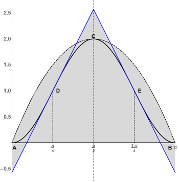
Figure 1: Four beautiful rules.

Let

$$I(f)=\displaystyle\int_{0}^{\pi}2\,\sin^{2}(x)dx=\pi\ .$$ (32)

In Figure 1 the graph of $f(x)=2\,\sin^{2}(x)$, passing through the points A,D,C,E, and B is displayed in bold. The simple rules $L,R,M,T,S$ and $T2$ are useless as approximations of the transcendental number $\pi$, since

$$L(f)=R(f)=0\quad\mbox{and}\quad M(f)=(\pi-0)f(\pi/2)=2\,\pi\ .$$

As $T=(L+R)/2$ and $S=(2\,T+M)/3$, we have

$$T(f)=0\quad\mbox{and}\quad S(f)=\displaystyle\frac{2\,\pi}{3}\ .$$

Taking into account that $f^{\prime\prime}(x)=4\,\cos(2\,x)$, the Taylor’s rule $T2$ is

$$T2(f)=M+\displaystyle\frac{\pi^{3}}{24}\,f^{\prime\prime}(\pi/2)=M-\pi^{3}/6=\pi\,(2-\pi^{3}/6)\ .$$

Recall that $Q_{n}$ denotes a composite rule with $n$ subintervals of $[a,b]$. The symmetry of the function with respect to the axis $x=\pi/2$ leads to the remarkable property that all the composite rules with $n=2$ subintervals, $L_{2},R_{2},M_{2}$ and the trapezoidal rule $T_{2}$, produce the exact value of (32), that is, $\pi$. The subintervals to be considered are $[0,\pi/2]$ and $[\pi/2,\pi]$. Thus,

$$\begin{array}[]{ll}L_{2}(f)&=0+\displaystyle\frac{\pi}{2}\times 2=\pi\quad\mbox{(left),}\\ \\ R_{2}(f)&=\displaystyle\frac{\pi}{2}\times 2+0=\pi\quad\mbox{(right),}\\ \\ T_{2}(f)&=\displaystyle\frac{\pi+\pi}{2}=\pi\quad\mbox{(trapezoidal),}\\ \\ M_{2}(f)&=\displaystyle\frac{\pi}{2}\times f\left(\displaystyle\frac{\pi}{4}\right)+\displaystyle\frac{\pi}{2}\times f\left(\displaystyle\frac{\pi}{4}\right)=\pi\quad\mbox{(midpoint)}\ .\\ \end{array}$$

The simple Simpson’s rule ($n=2$ subintervals) is not exact, as suggested by Figure 1 where the graphic of the interpolating polynomial passing trough the points A, C, B is displayed using a dashed line. It is obvious that the area delimited by the graph of the interpolating polynomial and the $x$-axis is not the same as the area under the graph of $f$. However, since the composite rule $M_{2}$ and $T_{2}$ are exact, the composite Simpson’s rule $S_{4}$, with $n=4$ subintervals, should be exact because this rule is a weighted mean of $M_{2}$ and $T_{2}$ given by (26). In fact,

$$\begin{array}[]{l}S_{2}(f)=\displaystyle\frac{2\,T(f)+M(f)}{3}=\displaystyle\frac{M(f)}{3}=\displaystyle\frac{2\,\pi}{3}\neq\pi,\end{array}$$

while

$$\begin{array}[]{l}S_{4}(f)=\displaystyle\frac{2\,T_{2}(f)+M_{2}(f)}{3}=\displaystyle\frac{3\,\pi}{3}=\pi\ .\end{array}$$

As shown previously that the simple Taylor’s rule $T2$ is not exact. However, the composite rule with $n=2$ subintervals is. Let us consider first the subinterval $[0,\pi/2]$. $T2$ represents the area delimited by the $x$-axis and the line segment (passing through the point D in Fig.1), whose cartesian equation is

$$y=f(\pi/4)+f^{\prime}(\pi/4)\,(x-\pi/4)=1+2\,(x-\pi/4),\quad 0\leq x\leq\pi/2,$$

Noting that $f^{\prime\prime}(\pi/4)=0$, we have

$$T2(f)=\displaystyle\pi/2\,f(\pi/4)=\displaystyle\frac{\pi}{2}\ .$$

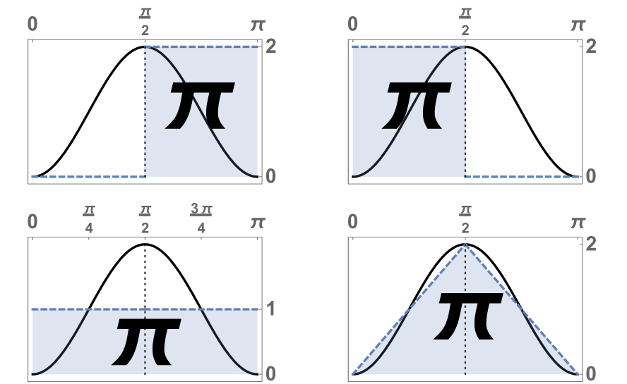
Figure 2: The four beautiful rules $L_{2},R_{2},M_{2}$ and $T_{2}$.

Analogously, in the subinterval $[\pi/2,\pi]$, the value of $T2$ represents the area delimited by the $x$-axis and the line segment (passing through the point E in Fig.1), whose cartesian equation is

$$y=f(3\,\pi/4)+f^{\prime}(3\,\pi/4)\,(x-3\,\pi/4)=1-2\,(x-3\,\pi/4),\quad\pi/2\leq x\leq\pi\ .$$

As $f^{\prime\prime}(3\,\pi/4)=0$, we obtain

$$T2(f)=\displaystyle\pi/2\,f(3\,\pi/4)=\displaystyle\frac{\pi}{2}\ .$$

Thus, the composite rule, with $n=2$, subintervals gives

$$T2_{2}(f)=\displaystyle\frac{\pi}{2}+\displaystyle\frac{\pi}{2}=\pi\ .$$

So, all the above six composite rules, $L_{n},R_{n},M_{n},T_{n},S_{n},T2_{n}$, with $n\geq 4$, are exact for the integral (32). In Figure 2 four plane regions whose area is $\pi$ are shown, giving a geometrical interpretation of the rules $L_{2}$, $R_{2}$, $M_{2}$ and $T_{2}$ respectively.

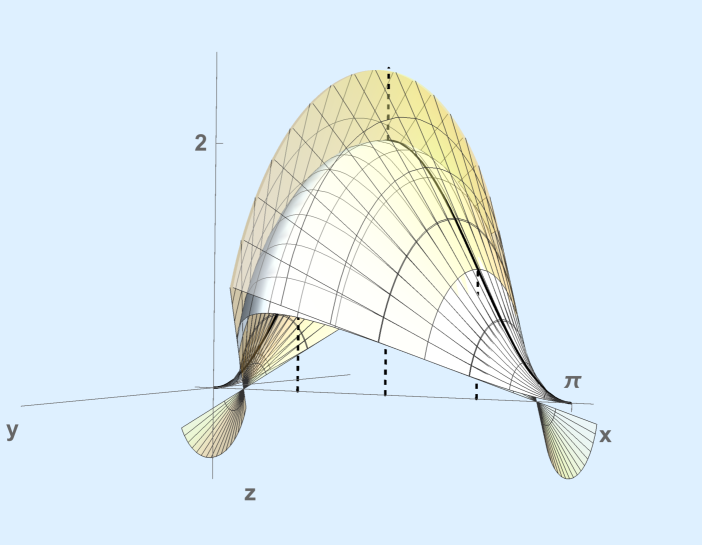
Figure 3: Partial revolution around the $x$ axis.

In Figure 3 we show (partial) surfaces generated by the revolution of the graphic $f$ around the $x$-axis together with the line segments (cf. Figure 1). This suggests interesting architectural applications of our companion and associate rules.

Example 2.

Let

$$I(f)=\displaystyle\int_{0}^{1/2}\displaystyle\frac{6}{\sqrt{1-x^{2}}}\,dx=\pi\ .$$

As the function $f(x)=6/\sqrt{1-x^{2}}$ is positive and its derivative is nonnegative derivative in $[0,1/2]$, the function $f$ is an increasing function. Therefore, for each $n\geq 1$, the rules $L_{n}$ and $R_{n}$ have errors of opposite signs and

$$L_{n}(f)\leq I(f)\leq R_{n}(f),\quad\forall n\geq 1\ .$$ (33)

As

$$R_{n}(f)-L_{n}(f)=\displaystyle\frac{(b-a)}{n}\,\left(f(b)-f(a)\right)=\displaystyle\frac{1}{2\,n}\,(4\sqrt{3}-6),$$

we have,

$$\lim_{n\rightarrow\infty}|R_{n}(f)-L_{n}(f)|=0\ .$$

Thus, from (33) it follows

$$\lim_{n\rightarrow\infty}R_{n}(f)=\lim_{n\rightarrow\infty}L_{n}(f)=\lim_{n\rightarrow\infty}=I(f)=\pi\ .$$

As the composite rule $T_{n}$ is the weighted mean (20) of $L_{n}$ and $R_{n}$, one concludes that $\lim_{n\rightarrow\infty}T_{n}(f)=\pi$. Moreover, as $f$ is an increasing function, we also have for the midpoint rule

$$L_{n}(f)\leq M_{n}(f)\leq R_{n}(f),\quad\forall n\geq 1\ .$$

Consequently, all the rules $L_{n},R_{n},M_{n},T_{n}$ have $\pi$ as common limit. The same is true for the Simpson rule $S_{n}$ since this is the weighted mean (26) between the composite companion rules $M_{n}$ (midpoint) and $T_{n}$ (trapezoidal).

Figure 4: Composite rules for $\displaystyle\int_{0}^{1/2}\displaystyle\frac{6}{\sqrt{1-x^{2}}}\,dx$ .

In Figure 4 we compare the errors for each of the previous rules, including the Taylor’ s rule $T2$. For $n=1,2,2^{2},2^{3},\ldots$ we firstly compute the 6-uple $(L_{n},R_{n},M_{n},T_{n},S_{n},T2_{n})$ using the following Mathematica code

L[f_, a_, b_] := (b - a) f[a];
R[f_, a_, b_] := (b - a) f[b];
M[f_, a_, b_] := (b - a) f[(a + b)/2];
T[f_, a_, b_] := (b - a)/2 (f[a] + f[b]);
S[f_, a_, b_] := (2 M[f, a, b] + T[f, a, b])/3;
T2[f_, a_, b_] := M[f, a, b] + (b - a)^2/24 f’’[(a + b)/2];
composite[rule_String, a_, b_, n_] := Block[{h},
   h = (b - a)/n // N;
   Total[Map[ToExpression[rule][f, #[[1]], #[[2]] ] &,
      Partition[Range[a, b, h], 2, 1]]    ] ];
 

The numerical values obtained from the 6 rules are sorted in increasing order. For each $n$, the second column of Figure 4 displays a string reflecting the names of the rule with respect to the order of the computed values. For instance the string LMSTT2R means that the smaller computed value is given by the (composite) left rectangle rule $L_{n}$ and the greatest one corresponds to the right rectangle rule $R_{n}$. The values in the columns Error Xi refer to the error of the rule in the $i$-th position of the respective string of rules names.

All the error columns in Fig. 4 show that the respective rule produce monotone sequences. Also, it is clear that $(L_{n},R_{n})$ and $(M_{n},T_{n})$ are pairs of companion rules. As the absolute error of $S_{n}$ is less than the one of $T2_{n}$, Simpson’s rule performs better than Taylor’s $T2$ and all the other rules.

Example 3.

Let

$$I(f)=\displaystyle\int_{-1}^{1}\displaystyle\frac{2}{1+x^{2}}\,dx=\pi\ .$$

Figure 5: Composite rules for $\displaystyle\int_{-1}^{1}\displaystyle\frac{2}{1+x^{2}}\,dx=\pi$ .

In this case $f(x)=2/(1+x^{2})$ is a positive function, symmetric with respect to the $y$-axis. The function increases from $x=-1$ to $x=0$ and decreases from $x=0$ to $x=1$. Both the function and its derivatives are bounded in $[-1,1]$. As shown in Figure 5, for $1\leq n\leq 4$ the composite rules $L_{n}$ and $M_{n}$ (midpoint) have errors of opposite sign, whilst for $8\leq n\leq 32$ the rules $T2_{n}$ and $M_{n}$ enjoy the same property. For all 6 rules their absolute errors seem to approach zero, as expected.

One can verify that for $n=2^{10}=1024$ the Simpson’s rule gives $\pi\simeq 3.1415926535897932384$, where all digits are correct.

References

- [1] M. Abramowitz, I. A. Stegun, Handbook of Mathematical Functions with Formulas, Graphs and Mathematical Tables, Dover, 1972.
- [2] H. Engels, Numerical quadrature and cubature, Academic Press, London, 1980.
- [3] P. J. Davis, P. Rabinowitz, Methods of Numerical Integration, Academic Press, Orlando, 1984.
- [4] C. F. Gauss, Methodus nova integralium valores per approximationem inveniendi, Commentationes Societatis Regiae Scientarium Gottingensis Recentiones 2, [Werke III], 123-162, 1812.
- [5] W. Gautschi, Numerical Analysis, An Introduction, Birkhauser, Boston, 1997.
- [6] M. M. Graça, Regras companheiras de Simpson-Milne, Boletim da Sociedade Portuguesa de Matemática, (in portuguese, to appear).
- [7] V. I. Krylov, Approximate Calculation of Integrals, Dover Pub., New York, 2005.
- [8] A. R. Krommer, C. W. Ueberhuber, Computational Integration, SIAM, Philadelphia, 1998.
- [9] I. Newton, Treatise of the Quadrature of Curves, in Sir Isaac Newton’s Two Treatises of The Quadrature of Curves, and Analysis by Equations of an infinite Number of Terms, by John Stewart, James Bettenham, London, 1745.
- [10] S. Nikolski, Fórmulas de Cuadratura, Editorial MIR, Moscú, 1990 (spanish version).
- [11] A. H. Stroud, D. Secrest Gaussian Quadrature Formulas, Prentice-Hall, Englewood Cliffs, N. J., 1966.
- [12] E. Suli, D. Mayers, An Introduction to Numerical Analysis, Cambridge University Press, New York, 2003.
- [13] E. T. Whittaker, G. Robinson, The Calculus of Observations, 3rd. ed., Blackie and Son, London, 1942.
- [14] S. Wolfram, The Mathematica Book, Wolfram Media, fifth ed., 2003.