Corrections to sink strengths used in rate equation simulations of defects in solids

Abstract

The mean-field rate equations have proven to be a versatile method in simulating defect dynamics and temporal changes in the micro-structure of materials. However, the reliability and usefulness of the method depends critically on the defect interaction parameters used. In this study, we show that the sink strength depends also on the detrapping or dissociation process. The sink strength for a defect that is detrapped, is much larger than the values usually used. We present a theory how to determine the appropriate sink strength, and show that the rate equation method, in some cases, gives wrong results if the detrapping dependence on the sink strength parameter is omitted.

The physical and mechanical properties of materials are largely controlled by their micro structure and defect and impurity concentrations. To understand and control these changes during ageing, ion irradiation or annealing, requires a long time and length scale simulation technique. The only simulation techniques that are able to fulfil these demanding scales are the mean-field rate equations and kinetic Monte Carlo (KMC) methods. The KMC is a stochastic simulation method, where all the dynamic properties and reactions for all involved defects have to be known. The strengths of this method include the ability to take into account expected and unexpected correlated events, e.g. close Frenkel pair annihilation. However, the time step for the KMC method might be of the order of 10^-11 s with only one self-interstitial atom in the system Derlet et al. (2007), which restricts the accessible time and defect concentrations for this method.

In the mean-field rate equations (RE) all the relevant defect mobilities and reactions are collected to a set of non-linear differential equations that are solved in time and space McNabb and Foster (1963); Wiedersich (1972); Freeman (1987); Ahlgren et al. (2012). RE has been extensively used for simulating different dynamic processes in materials. These studies include finding trapping energies of He and H in vacancies Baskes and Wilson (1983); Myers et al. (1983), clustering of irradiation induced vacancies and self-interstitials Wiedersich (1972), He and H bubble formation Wilson et al. (1976), swelling Brailsford and Bullough (1972), precipitation Wert and Zener (1949), fusion edge localized modes simulations Heinola et al. (2019), H isotope exchange Schmid et al. (2014); Hodille et al. (2016); Markelj et al. (2016) and simulation of thermal desorption spectrometry (TDS) profiles Pisarev et al. (2003); Poon et al. (2008); Gasparyan et al. (2015); Hodille et al. (2016), to mention just a few.

The dynamic processes and reactions for all involved defects have to be known also for the RE method. The trapping or annihilation processes are described by the so called sink strength McNabb and Foster (1963); Brailsford and Bullough (1972); Wiedersich (1972), and the detrapping or dissociation processes by the detrapping parameter. The detrapping parameters can be determined by reaction rate theory Arrhenius (1889) and transition state theory Wigner (1932); Eyring (1935).

The sink strengths have been determined analytically for various symmetric traps including spherical traps, dislocation lines and grain boundaries Wert and Zener (1949); Brailsford and Bullough (1981); Wiedersich (1972); Rouchette et al. (2014). For arbitrarily shaped traps the Monte Carlo (MC) method can to be used Malerba et al. (2007); Jansson et al. (2013); Ahlgren and Bukonte (2017). The sink strength dependence on the trap volume fraction and defect jump length using a fast MC method is developed in Ref. Ahlgren and Bukonte (2017). The sink strength also depends on the dimensionality of diffusion Borodin (1998); Trinkaus et al. (2002). The effect of the strain field between the defect and trap trap can also be taken into account Doan and Martin (2003); Ahlgren et al. (2012).

The main advantage of the RE method is that it is a very fast method to be used for long time and length scale simulations. However, the usefulness of the simulation results depend critically on that the defect interaction parameters, i.e. sink strengths are correct. In this paper, we show that the sink strength actually depends on the detrapping or dissociation process. We further show that the RE method, in some cases, gives wrong results if the detrapping dependence on the sink strength parameter is omitted.

The rate equation and sink strength theories are developed in Refs. Wert and Zener (1949); McNabb and Foster (1963); Brailsford and Bullough (1972); Wiedersich (1972). We want to relate the concentration change in time of a diffusing defect $c$ (cm^-3) due to trapping and detrapping processes. The simplified rate equation with only one kind of trap and excluding boundary diffusion (constant total $c$ concentration) and source terms for brevity is given by:

$$\frac{dc}{dt} = -c_{e}\oint F^{in}dA+c_{f}\oint F^{out}dA$$ (1)

$$= -Dkc+E$$

where $c_{e}$ and $c_{f}$ are the concentrations of empty and filled traps, $F^{in}$ and $F^{out}$ are the fluxes of defect $c$ into and out from the traps. $c_{e}\oint F^{in}dA$ and $c_{f}\oint F^{out}dA$ denote the trapped and detrapped defect concentrations per second, where $A$ is the trap surface area. The trapped defect concentration per second is proportional to the defect concentration $c$, its diffusion coefficient $D$ (cm²/s) and the sink strength $k$ (cm^-2). $E$ is the thermal emission (detrapping) of defect $c$ from filled trap $c_{f}$, which from rate theory is:

$$E=c_{f}\nu\ \text{exp}\left(-\frac{E_{t}}{k_{B}T}\right),$$ (2)

where $\nu$ is the detrapping attempt frequency (Hz), $E_{t}$ ($\approx E_{b}+E_{m}$) is the trapping or dissociation energy (eV), $E_{b}$ is the binding energy and $E_{m}$ the defect migration barrier, $k_{B}$ is the Boltzmann constant and $T$ the absolute temperature.

Usually, the sink strength is determined analytically or by the MC method and the detrapping attempt frequency and the trapping energy from atomistic simulations or experiments. The analytical sink strength for spherical traps under 3D diffusion limit with trap radius $R_{t}$ and concentration $c_{e}$ is given by the recursive equation by Brailsford and Bullough Brailsford and Bullough (1981):

$$k=4\pi R_{t}c_{e}(1+R_{t}\sqrt{k}).$$ (3)

A modified equation taking into account the trap volume fraction and defect jump length is given in Ahlgren and Bukonte (2017). The sink strengths are defined for randomly distributed defects which results, for instance, from irradiation. However, if the defects detrap from traps, the initial position is located close to the trap. We will now show that the sink strength for defects is greatly enhanced if the initial location close to the trap is taken into account.

The sink strengths for spherical traps are simulated by the fast MC method Ahlgren and Bukonte (2017). The initial position for the defect in the cell is either random or a close distance (0.05 nm) from the trap boundary, as if the defect would have been detrapped. The trap and MC parameters are given in Table 1. The concentrations of the traps was chosen so that the trap volume fraction is approximately between 5$\times 10^{-6}$ and 0.2.

Table 1: The parameters used for MC sink strength simulations. The defect jump length is 0.1 nm and 10⁷ defects are simulated for each trap concentration giving a statistical error of about 3$\times 10^{-4}$% for the sink strengths Ahlgren and Bukonte (2017).

Trap radius	Trap concentration
(nm)	(nm-3)
0.5	6$\times 10^{-6}$ - 0.4
1.0	7$\times 10^{-6}$ - 5$\times 10^{-2}$
2.0	1$\times 10^{-7}$ - 6$\times 10^{-3}$

The results for the sink strength simulations are shown in Fig. 1. The defects with close to trap initial position have a large probability to be trapped in the trap close to it before diffusing away from it. Thus, the sink strength is much larger for defects close to the trap than for defects with random initial position. Note also that the usually used random sink strength, Eq. (3), is about 50% too small at the highest trap volume fraction.

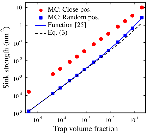
Figure 1: The sink strengths for spherical trap with trap radius 1.0 nm simulated by MC. The initial position for the defect in the simulation cell is either random or a close distance (0.05 nm) from the trap boundary. The sink strengths for defects with close to trap initial position is greatly enhanced compared to the ones with random initial position.

Figure 2 shows, for three different trapping radii: 0.5, 1.0 and 2.0 nm, the enhancement factor, which is defined as the sink strength for close position divided by the strength for random position. The probability to be trapped in the close trap increases with the trap size. Therefore, the enhancement factor increases with larger traps. The enhancement factor approaches a maximum value when the trap concentration goes to zero. For larger trap volume fractions, the trap concentration is larger and the probability to be trapped in another trap than the close one increases, leading to a smaller enhancement factor.

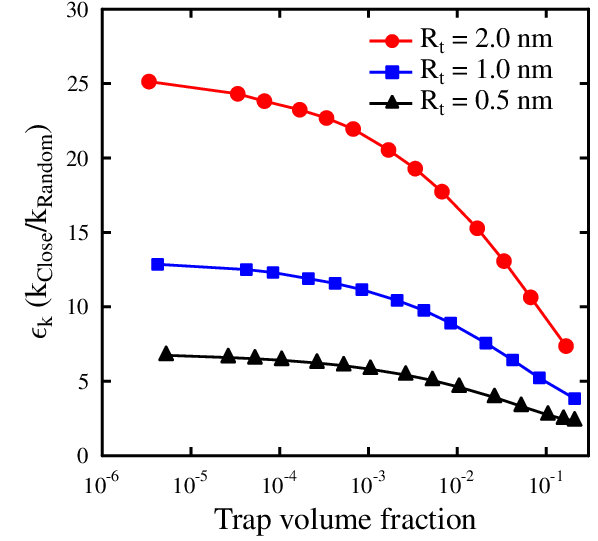
Figure 2: The enhancement factor $\epsilon_{k}$ (sink strength for close position divided by the sink strength for random position) as a function of trap volume fraction for three different trapping radii. For trapping radius 1.0 nm, the points are from the sink strengths given in Fig. 1.

The sink strengths are clearly larger if the defects are introduced in the cell from detrapping compared to irradiation. At equilibrium ($dc/dt=0$) the detrapping and trapping rates are equal and Eq. (1) gives

$$Dkc=E=c_{e}\oint F^{in}dA=\epsilon_{k}c_{f}\oint F^{out}dA,$$ (4)

which takes into account the enhancement, $\epsilon_{k}$, due to close detrapping. From this we get

$$c_{f}\oint F^{out}dA=E/\epsilon_{k},$$ (5)

which inserted in the sink strength solved from Eq. (1) becomes

$$k = \frac{1}{D\ c}\left[c_{e}\oint F^{in}dA-c_{f}\oint F^{out}dA+E\right]$$ (6)

$$= \frac{1}{D\ c}\left[c_{e}\oint F^{in}dA-E/\epsilon_{k}+E\right]$$

$$= \frac{c_{e}}{D\ c}\oint F^{in}dA+\frac{E(1-1/\epsilon_{k})}{D\ c}$$

$$= k_{rand}+\frac{E(1-1/\epsilon_{k})}{D\ c}.$$

The first term is the usual random position sink strength Brailsford and Bullough (1972); Wiedersich (1972) and the second term start enhancing the sink strength when detrapping is activated. If there is no detrapping or the enhancement factor is one, the sink strength reduces to the one usually used. The full rate equation including 3D diffusion and the source of defects (S) from irradiation now reads

$$\frac{dc}{dt} = D\nabla^{2}c-Dkc+E+S,$$ (7)

where the $k$ is given in Eq. (6). An alternative formulation that gives the right equilibrium condition, with the irradiation term omitted, is obtained if Eq. (6) is inserted in Eq. (7)

$$\frac{dc}{dt} = D\nabla^{2}c-Dk_{rand}c+E/\epsilon_{k}.$$ (8)

This alternative form should only be used without the source term.

To check the RE simulation results using different sink strength theories, we do the following test simulation, where the parameters have been chosen so that KMC simulations are possible to do for comparison. We have a 200 nm thick layer with a Gaussian trap profile located at the mean depth 50 nm, standard deviation (SD) 10 nm and the maximum trap concentration value at the mean depth is 1$\times 10^{18}$ $cm^{-3}$. Initially the traps are filled with the defects, with one defect per trap. The different parameters used in the simulations are given in Table 2. The $k_{rand}$ is given by Eq. (3). The difference in using Eq. (3) or the sink strength from Ahlgren and Bukonte (2017) is very small, because of the low trap volume fraction seen in Fig. 1. The temperature in the beginning of the simulation is 300 K and increases linearly with 50 K/s to 800 K during the 10 s simulation. With increasing temperature in the simulation, defects start to detrap and diffuse in the layer. Some of them are retrapped but some reach the surface and leave the layer. This defect surface flux away from the layer is monitored and compared for the RE and KMC simulations. The simulation corresponds to the popular thermal desorption spectrometry (TDS) method frequently used in experiments and simulations. Here, there are no surface parameters, the flux of defects is calculated directly as the flux ($cm^{-2}s^{-1}$) of atoms crossing the layer boundary. In the second simulation we use two different traps to see the effect of traps with different trapping energies. The defect diffusion parameters for all the simulations are: jump length 0.1 nm, jump frequency 5$\times 10^{12}$Hz and migration barrier 0.25 eV. The detrapping distance from the traps is 0.05 nm. Both traps have the Gaussian mean depth 50 nm with standard deviation 10 nm.

Table 2: The trap parameters used for RE and KMC test simulations. Only trap 1 is used in the first simulation and both traps in the second one. The defect detrapping attempt frequency $\nu$ is 5$\times 10^{12}$ Hz for both traps. R_t is the trapping radius and E_b the binding energy.

Trap	Gaussian	Rt	Eb
Num.	Max. conc. ($cm^{-3}$)	(nm)	(eV)
1:	1$\times 10^{18}$	1.0	0.8
2:	5$\times 10^{17}$	2.0	1.0

Figure 3 shows the KMC and RE simulated fluxes of the detrapped and diffusing defects through the front surface. The RE is now 1D with depth $z$ in the layer and reads

$$\frac{dc}{dt} = D\frac{d^{2}c}{dz^{2}}-Dkc+E.$$ (9)

The different sink strengths and detrapping terms used are given in Table 3.

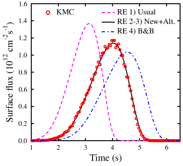
Figure 3: The defect flux comparison between KMC and RE simulations using different sink strength theories (see text).

We can see that the TDS peak (defect flux through the front surface) occurs too fast for the usual RE formalism. This is to be expected because the sink strength is too small, it does not take into account the enhanced retrapping due to the defects being detrapped close to the empty trap. The new theory Eq. (7) and the equivalent formulation Eq. (8) matches nicely with the KMC simulations. However, even if the TDS peak for Eq. (7) and Eq. (8) are almost identical, their defect profile in the layer during the simulation is not. Eq. (7) agrees with the KMC defect profile during the simulation, detrapping starts similar to KMC and the enhanced trapping delays the defect diffusion away from the trap profile. Whereas for Eq. (8) the detrapping is delayed, which in a similar way delays the defect diffusion away from the trap profile. Using the equations by Brailsford & Bullough Brailsford and Bullough (1981) gives the TDS peak too late.

Table 3: The sink strengths and detrapping terms used for the RE test simulations. $k_{rand}$ is given by Eq. (3).

	Sink strength,$k$	Detrapping, $E$
1) Usual	$k_{rand}$	$c_{f}\nu\ \text{exp}(-E_{t}/k_{B}T)$
2) New	$k_{rand}+E(1-1/\epsilon_{k})/(D\ c)$	$c_{f}\nu\ \text{exp}(-E_{t}/k_{B}T)$
3) New (Alt)a	$k_{rand}$	$c_{f}\nu\ \text{exp}(-E_{t}/k_{B}T)/\epsilon_{k}$
4) B&Bb	$k_{rand}$	$4\pi R_{t}c_{f}(1+R_{t}\sqrt{k})D\text{exp}(-E_{b}/k_{B}T)$

^a Alternative formulation Eq. (8).
^b Brailsford & Bullough Brailsford and Bullough (1981).

The simulation with two traps, Fig. 4, confirms the results for the one trap simulation. Eq. (7) and Eq. (8) agree with the KMC simulations, while the TDS peaks are shifted for the other formulations. The apparent TDS agreement between times 7 and 8 s for the B&B formulation is a coincidence. Because, the detrapping term in Table 3 with the diffusion coefficient, $D=1/6\cdot 0.1^{2}\nu\cdot\text{exp}(-E_{m}/k_{B}T)$, approximately becomes: $4\pi 2c_{f}(1/6\cdot 0.1^{2}\nu)\text{exp}(-E_{t}/k_{B}T)\approx c_{f}\nu\ \text{exp}(-E_{t}/k_{B}T)/24$, which happens to agree with the alternative formulation Table 3, for the enhancement factor for trapping radius 2 nm from Fig. 2. The diffusion jump and the detrapping frequencies are the same in these simulations. It should be noted that even though the simulation was chosen favourable for the KMC technique, the RE simulation was about 100000 faster.

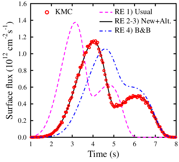
Figure 4: The defect flux comparison between KMC and RE simulations with two traps.

The results of this study show that the sink strengths can also depend on the detrapping or dissociation process. Therefore, the numerous simulations including detrapping, done for about 50 years are probably not entirely accurate. The new sink strength formulation needs the new enhancement factor parameter to be determined. The enhancement factor can easily be obtained using the MC method, and Fig. 4 shows that the factors don’t affect each other for trap concentrations below about 1$\times 10^{18}$ $cm^{-3}$. However, if the different trap concentrations are higher, then the effect of the other traps on each enhancement factor has to be checked. Including the detrapping effect in the sink strength interaction parameter will take usefulness of the RE method to a new level. The RE simulations should now give more reliable defect and trap parameters, and the long length and time scale micro structure simulations should be more accurate.

References

References

- Derlet et al. (2007) P. M. Derlet, D. Nguyen-Manh, and S. L. Dudarev, Phys. Rev. B 76, 054107 (2007).
- McNabb and Foster (1963) A. McNabb and P. K. Foster, Trans. Metal. Soc. AIME 227, 618 (1963).
- Wiedersich (1972) H. Wiedersich, Radiation Effects 12, 111 (1972).
- Freeman (1987) G. Freeman, Kinetics of nonhomogeneous processes, L.K. Mansur: Mechanisms and Kinetics of Radiation Effects in Metals and Alloys (John Wiley and Sons, New York, NY, 1987).
- Ahlgren et al. (2012) T. Ahlgren, K. Heinola, K. Vörtler, and J. Keinonen, Journal of Nuclear Materials 427, 152 (2012).
- Baskes and Wilson (1983) M. I. Baskes and W. D. Wilson, Phys. Rev. B 27, 2210 (1983).
- Myers et al. (1983) S. M. Myers, P. Nordlander, F. Besenbacher, and J. K. Nørskov, Phil. Mag. A 48, 397 (1983).
- Wilson et al. (1976) W. D. Wilson, M. I. Baskes, and C. L. Bisson, Phys. Rev. B 13, 2470 (1976).
- Brailsford and Bullough (1972) A. Brailsford and R. Bullough, J. Nucl. Mater. 44, 121 (1972).
- Wert and Zener (1949) C. Wert and C. Zener, J. Appl. Phys. 21, 5 (1949).
- Heinola et al. (2019) K. Heinola, T. Ahlgren, S. Brezinsek, T. Vuoriheimo, and S. Wiesen, Nuclear Materials and Energy 19, 397 (2019).
- Schmid et al. (2014) K. Schmid, U. von Toussaint, and T. Schwarz-Selinger, Journal of Applied Physics 116, 134901 (2014).
- Hodille et al. (2016) E. A. Hodille, Y. Ferro, N. Fernandez, C. S. Becquart, T. Angot, J. M. Layet, R. Bisson, and C. Grisolia, Physica Scripta 2016, 014011 (2016).
- Markelj et al. (2016) S. Markelj, A. Založnik, T. Schwarz-Selinger, O. Ogorodnikova, P. Vavpetič, P. Pelicon, and I. Čadež, Journal of Nuclear Materials 469, 133 (2016).
- Pisarev et al. (2003) A. A. Pisarev, I. D. Voskresensky, and S. I. Porfirev, J. Nucl. Mater. 313–316, 604 (2003).
- Poon et al. (2008) M. Poon, A. Haasz, and J. Davis, J. Nucl. Mater. 374, 390 (2008).
- Gasparyan et al. (2015) Y. Gasparyan, O. Ogorodnikova, V. Efimov, A. Mednikov, E. Marenkov, A. Pisarev, S. Markelj, and I. Čadež, Journal of Nuclear Materials 463, 1013 (2015).
- Arrhenius (1889) S. Arrhenius, Z. Phys. Chem. (Leipzig) 4, 226 (1889).
- Wigner (1932) E. Wigner, Z. Phys. Chem. Abt. 19, 203 (1932).
- Eyring (1935) H. Eyring, J. Chem. Phys. 3, 107 (1935).
- Brailsford and Bullough (1981) A. D. Brailsford and R. Bullough, Philos. Trans. R. Soc. London 302, 87 (1981).
- Rouchette et al. (2014) H. Rouchette, L. Thuinet, A. Legris, A. Ambard, and C. Domain, Computational Materials Science 88, 50 (2014).
- Malerba et al. (2007) L. Malerba, C. S. Becquart, and C. Domain, J. Nucl. Mater. 360, 159 (2007).
- Jansson et al. (2013) V. Jansson, L. Malerba, A. D. Backer, C. S. Becquart, and C. Domain, J. Nucl. Mater. 442, 218 (2013).
- Ahlgren and Bukonte (2017) T. Ahlgren and L. Bukonte, Journal of Nuclear Materials 496, 66 (2017).
- Borodin (1998) V. Borodin, Physica A: Statistical Mechanics and its Applications 260, 467 (1998).
- Trinkaus et al. (2002) H. Trinkaus, H. L. Heinisch, A. V. Barashev, S. I. Golubov, and B. N. Singh, Phys. Rev. B 66, 060105 (2002).
- Doan and Martin (2003) N. V. Doan and G. Martin, Phys. Rev. B 67, 134107 (2003).