Research
 
Detecting problematic transactions in a consumer-to-consumer e-commerce network
 
Shun Kodate^1,2, Ryusuke Chiba³, Shunya Kimura³, Naoki Masuda^4,5,2*
 
* Corresponding author
naokimas@buffalo.edu

1 Graduate School of Information Sciences, Tohoku University, Sendai, 980-8579, Japan
2 Department of Engineering Mathematics, University of Bristol, Bristol, BS8 1UB, UK
3 Mercari, Inc., Tokyo, 106-6118, Japan
4 Department of Mathematics, University at Buffalo, Buffalo, NY, 14260-2900, USA
5 Computational and Data-Enabled Science and Engineering Program, University at Buffalo, Buffalo, NY, 14260-5030, USA

S.Kodate: kodate@sb.ecei.tohoku.ac.jp
RC: metalunk@mercari.com
S.Kimura: kimuras@mercari.com
NM: naokimas@buffalo.edu

Abstract
Providers of online marketplaces are constantly combatting against problematic transactions, such as selling illegal items and posting fictive items, exercised by some of their users. A typical approach to detect fraud activity has been to analyze registered user profiles, user’s behavior, and texts attached to individual transactions and the user. However, this traditional approach may be limited because malicious users can easily conceal their information. Given this background, network indices have been exploited for detecting frauds in various online transaction platforms. In the present study, we analyzed networks of users of an online consumer-to-consumer marketplace in which a seller and the corresponding buyer of a transaction are connected by a directed edge. We constructed egocentric networks of each of several hundreds of fraudulent users and those of a similar number of normal users. We calculated eight local network indices based on up to connectivity between the neighbors of the focal node. Based on the present descriptive analysis of these network indices, we fed twelve features that we constructed from the eight network indices to random forest classifiers with the aim of distinguishing between normal users and fraudulent users engaged in each one of the four types of problematic transactions. We found that the classifier accurately distinguished the fraudulent users from normal users and that the classification performance did not depend on the type of problematic transaction.
 
Keywords:
Network analysis; Machine learning; Fraud detection; Computational social science

Introduction

In tandem with the rapid growth of online and electronic transactions and communications, fraud is expanding at a dramatic speed and penetrates our daily lives. Fraud including cybercrimes costs billions of dollars per year and threatens the security of our society [1, 2]. In particular, in the recent era where online activity dominates, attacking a system is not too costly, whereas defending the system against fraud is costly[3]. The dimension of fraud is vast and ranges from credit card fraud, money laundering, computer intrusion, to plagiarism, to name a few.

Computational and statistical methods for detecting and preventing fraud have been developed and implemented for decades [4, 5, 6, 7]. Standard practice for fraud detection is to employ statistical methods including the case of machine learning algorithms. In particular, when both fraudulent and non-fraudulent samples are available, one can construct a classifier via supervised learning [4, 5, 6, 7]. Exemplar features to be fed to such a statistical classifier include the transaction amount, day of the week, item category, and user’s address for detecting frauds in credit card systems, number of calls, call duration, call type, and user’s age, gender, and geographical region in the case of telecommunication, and user profiles and transaction history in the case of online auctions [6].

However, many of these features can be easily faked by advanced fraudsters[8, 9]. Furthermore, fraudulent users are adept at escaping the eyes of the administrators or authorities that would detect the usage of particular words as a signature of anomalous behavior [10, 11, 12]. For example, if the authority discovers that one jargon means a drug, then fraudulent users may easily switch to another jargon to confuse the authority.

Network analysis is an alternative way to construct features and is not new to fraud detection techniques[13, 8]. The idea is to use connectivity between nodes, which are usually users or goods, in the given data and calculate graph-theoretic quantities or scores that characterize nodes. These methods stand on the expectation that anomalous users show connectivity patterns that are distinct from those of normal users [8]. Network analysis has been deployed for fraud detection in insurance[14], money laundering[15, 16, 17], health-care data[18], car-booking[19], a social security system[20], mobile advertising[21], a mobile phone network[22], online social networks[23, 24, 25, 26], online review forums[27, 28, 29], online auction or marketplaces[30, 31, 32, 33, 34], credit card transactions[35, 36], cryptocurrency transaction[37], and various other fields[38]. For example, fraudulent users and their accomplices were shown to form approximately bipartite cores in a network of users to inflate their reputations in an online auction system[30]. Then, the authors proposed an algorithm based on a belief propagation to detect such suspicious connectivity patterns. This method has been proven to be also effective on empirical data obtained from eBay[31].

In the present study, we analyze a data set obtained from a large online consumer-to-consumer (C2C) marketplace, Mercari, operating in Japan and the US. They are the largest C2C marketplace in Japan, in which, as of 2019, there are 13 million monthly active users and 133 billion yen (approximately 1.2 billion USD) transactions per quarter year [39]. Note that we analyze transaction frauds based on transaction networks of users, which contrasts with previous studies of online C2C marketplaces that looked at reputation frauds [30, 31, 32, 34]. Many prior network-based fraud detection algorithms used global information about networks, such as connected components, communities, betweenness, $k$-cores, and that determined by belief propagation [30, 31, 32, 14, 27, 23, 22, 24, 33, 15, 35, 25, 18, 20, 16, 21, 36, 28, 17, 26, 19, 29]. Others used local information about the users’ network, such as the degree, the number of triangles, and the local clustering coefficient [30, 38, 14, 34, 33, 23, 15, 37, 20, 16]. We will focus on local features of users, i.e., features of a node that can be calculated from the connectivity of the user and the connectivity between neighbors of the user. This is because local features are easier and faster to calculate and thus practical for commercial implementations.

Materials and methods

Data

Mercari is an online C2C marketplace service, where users trade various items among themselves. The service is operating in Japan and the United States. In the present study, we used the data obtained from the Japanese market between July 2013 and January 2019. In addition to normal transactions, we focused on the following types of problematic transactions: fictive, underwear, medicine, and weapon. Fictive transactions are defined as selling non-existing items. Underwear refers to transactions of used underwear; they are prohibited by the service from the perspective of morality and hygiene. Medicine refers to transactions of medicinal supplies, which are prohibited by the law. Weapon refers to transactions of weapons, which are prohibited by the service because they may lead to crime. The number of sampled users of each type is shown in Table 1.

Network analysis

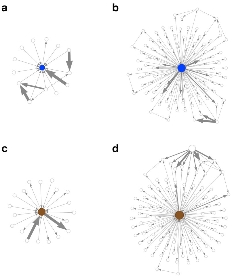
Figure 1: Examples of egocentric networks. (a) and (b): Egocentric networks of arbitrarily selected two normal users. (c) and (d): Egocentric networks of arbitrarily selected two fraudulent users involved in selling a fictive item.

We examine a directed and weighted network of users in which a user corresponds to a node and a transaction between two users represents a directed edge. The weight of the edge is equal to the number of transactions between the seller and the buyer. We constructed egocentric networks of each of several hundreds of normal users and those of fraudulent users, i.e., those engaged in at least one problematic sell. Figure 1 shows the egocentric networks of two normal users (Fig. 1a, b) and those of two fraudulent users involved in selling a fictive item (Fig. 1c, d). The egocentric network of either a normal or fraudulent user contained the nodes neighboring the focal user, edges between the focal user and these neighbors, and edges between the pairs of these neighbors.

We calculated eight indices for each focal node. They are local indices in the meaning that they require the information up to the connectivity among the neighbors of the focal node.

Five out of the eight indices use only the information about the connectivity of the focal node. The degree $k_{i}$ of node $v_{i}$ is the number of its neighbors. The node strength [40] (i.e., weighted degree) of node $v_{i}$, denoted by $s_{i}$, is the number of transactions in which $v_{i}$ is involved. Using these two indices, we also considered the mean number of transactions per neighbor, i.e., $s_{i}/k_{i}$, as a separate index. These three indices do not use information about the direction of edges.

The sell probability of node $v_{i}$, denoted by $\mathrm{SP}_{i}$, uses the information about the direction of edges and defined as the proportion of the $v_{i}$’s neighbors for which $v_{i}$ acts as seller. Precisely, the sell probability is given by

$$\mathrm{SP}_{i}=\frac{k_{i}^{\mathrm{out}}}{k_{i}^{\mathrm{in}}+k_{i}^{\mathrm{out}}},$$ (1)

where $k_{i}^{\mathrm{in}}$ is $v_{i}$’s in-degree (i.e., the number of neighbors from whom $v_{i}$ bought at least one item) and $k_{i}^{\mathrm{out}}$ is $v_{i}$’s out-degree (i.e., the number of neighbors to whom $v_{i}$ sold at least one item). It should be noted that, if $v_{i}$ acted as both seller and buyer towards $v_{j}$, the contribution of $v_{j}$ to both in- and out-degree of $v_{i}$ is equal to one. Therefore, $k_{i}^{\mathrm{in}}+k_{i}^{\mathrm{out}}$ is not equal to $k_{i}$ in general.

The weighted version of the sell probability, denoted by $\mathrm{WSP}_{i}$, is defined as

$$\mathrm{WSP}_{i}=\frac{s_{i}^{\mathrm{out}}}{s_{i}^{\mathrm{in}}+s_{i}^{\mathrm{out}}},$$ (2)

where $s_{i}^{\mathrm{in}}$ is node $v_{i}$’s weighted in-degree (i.e., the number of buys) and $s_{i}^{\mathrm{out}}$ is $v_{i}$’s weighted out-degree (i.e., the number of sells).

The other three indices are based on triangles that involve the focal node. The local clustering coefficient $C_{i}$ quantifies the abundance of undirected and unweighted triangles around $v_{i}$[41]. It is defined as the number of undirected and unweighted triangles including $v_{i}$ divided by $k_{i}(k_{i}-1)/2$. The local clustering coefficient $C_{i}$ ranges between 0 and 1.

We hypothesized that triangles contributing to an increase in the local clustering coefficient are localized around particular neighbors of node $v_{i}$. Such neighbors together with $v_{i}$ may form an overlapping set of triangles, which may be regarded as a community [42, 43]. Therefore, our hypothesis implies that the extent to which the focal node is involved in communities should be different between normal and fraudulent users. To quantify this concept, we introduce the so-called triangle congregation, denoted by $m_{i}$. It is defined as the extent to which two triangles involving $v_{i}$ share another node and is given by

$$m_{i}=\frac{\textrm{(Number of pairs of triangles involving $v_{i}$ that share another node)}}{\mathrm{Tr}_{i}(\mathrm{Tr}_{i}-1)/2},$$ (3)

where $\mathrm{Tr}_{i}=C_{i}k_{i}(k_{i}-1)/2$ is the number of triangles involving $v_{i}$. Note that $m_{i}$ ranges between 0 and 1.

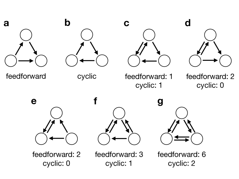
Figure 2: Directed triangle patterns and their count. (a) Feedforward triangle. (b) Cyclic triangle. (c)– (g) Five three-node patterns that contain directed triangles and reciprocal edges. The numbers shown in the figure represent the number of feedforward or cyclic triangles to which each three-node pattern contributes.

Frequencies of different directed three-node subnetworks, conventionally known as network motifs[44], may distinguish between normal and fraudulent users. In particular, among triangles composed of directed edges, we hypothesized that feedforward triangles (Fig. 2a) should be natural and that cyclic triangles (Fig. 2b) are not. We hypothesized so because a natural interpretation of a feedforward triangle is that a node with out-degree two tends to serve as seller while that with out-degree zero tends to serve as buyer and there are many such nodes that use the marketplace mostly as buyer or seller but not both. In contrast, an abundance of cyclic triangles may imply that relatively many users use the marketplace as both buyer and seller. We used the index called the cycle probability, denoted by $\mathrm{CYP}_{i}$, which is defined by

$$\mathrm{CYP}_{i}=\frac{\mathrm{CY}_{i}}{\mathrm{FF}_{i}+\mathrm{CY}_{i}},$$ (4)

where $\mathrm{FF}_{i}$ and $\mathrm{CY}_{i}$ are the numbers of feedforward triangles and cyclic triangles to which node $v_{i}$ belongs. The definition of $\mathrm{FF}_{i}$ and $\mathrm{CY}_{i}$, and hence $\mathrm{CYP}_{i}$, is valid even when the triangles involving $v_{i}$ have bidirectional edges. In the case of Fig. 2c, for example, any of the three nodes contains one feedforward triangle and one cyclic triangle. The other four cases in which bidirectional edges are involved in triangles are shown in Figs. 2d-g. In the calculation of $\mathrm{CYP}_{i}$, we ignored the weights of edges.

Random forest classifier

To classify users into normal and fraudulent users based on their local network properties, we employed a random forest classifier [45, 46, 47] implemented in scikit-learn[48]. It uses an ensemble learning method that combines multiple classifiers, each of which is a decision tree, built from training data and classifies test data avoiding overfitting. We combined 300 decision-tree classifiers to construct a random forest classifier. Each decision tree is constructed on the basis of training samples that are randomly subsampled with replacement from the set of all the training samples. To compute the best split of each node in a tree, one randomly samples the candidate features from the set of all the features. The probability that a test sample is positive in a tree is estimated as follows. Consider the terminal node in the tree that a test sample eventually reaches. The fraction of positive training samples at the terminal node gives the probability that the test sample is classified as positive. One minus the positive probability gives the negative probability estimated for the same test sample. The positive or negative probability for the random forest classifier is obtained as the average of single-tree positive or negative probability over all the 300 trees. A sample is classified as positive by the random forest classifier if the positive probability is larger than 0.5, otherwise classified as negative.

We split samples of each type into two sets such that 75% and 25% of the samples of each type are assigned to the training and test samples, respectively. There were more normal users than any type of fraudulent user. Therefore, to balance the number of the negative (i.e., normal) and positive (i.e., fraudulent) samples, we uniformly randomly subsampled the negative samples (i.e., under-sampling) such that the number of the samples is the same between the normal and fraudulent types in the training set.

Based on the training sample constructed in this manner, we built each of the 300 decision trees and hence a random forest classifier. Then, we examined the classification performance of the random forest classifier on the set of test samples.

The true positive rate, also called the recall, is defined as the proportion of the positive samples (i.e., fraudulent users) that the random forest classifier correctly classifies as positive. The false positive rate is defined as the proportion of the negative samples (i.e., normal users) that are incorrectly classified as positive. The precision is defined as the proportion of the truly positive samples among those that are classified as positive. The true positive rate, false positive rate, and precision range between 0 and 1.

We used the following two performance measures for the random forest classifier. To draw the receiver operating characteristic (ROC) curve for a random forest classifier, one first arranges the test samples in descending order of the estimated probability that they are positive. Then, one plots each test sample, with its false positive rate on the horizontal axis and the true positive rate on the vertical axis. By connecting the test samples in a piecewise linear manner, one obtains the ROC curve. The precision-recall (PR) curve is generated by plotting the samples in the same order in $[0,1]^{2}$, with the recall on the horizontal axis and the precision on the vertical axis. For an accurate binary classifier, both ROC and PR curves visit near $(x,y)=(0,1)$. Therefore, we quantify the performance of the classifier by the area under the curve (AUC) of each curve. The AUC ranges between 0 and 1, and a large value indicates a good performance of the random forest classifier.

To calculate the importance of each feature in the random forest classifier, we used the permutation importance [49, 50]. With this method, the importance of a feature is given by the decrease in the performance of the trained classifier when the feature is randomly permuted among the test samples. A large value indicates that the feature considerably contributes to the performance of the classifier. To calculate the permutation importance, we used the AUC value of the ROC curve as the performance measure of a random forest classifier. We computed the permutation importance of each feature with ten different permutations and adopted the average over the ten permutations as the importance of the feature.

We optimized the parameters of the random forest classifier by a grid search with 10-fold cross-validation on the training set. For the maximum depth of each tree (i.e., the max_depth parameter in scikit-learn), we explored the integers between 3 and 10. For the number of candidate features for each split (i.e., max_features), we explored the integers between 3 and 6. For the minimum number of samples required at terminal nodes (i.e., min_samples_leaf), we explored 1, 3, and 5. As mentioned above, the number of trees (i.e., n_estimators) was set to 300. The seed number for the random number generator (i.e., random_state) was set to 0. For the other hyperparameters, we used the default values in scikit-learn version 0.22. In the parameter optimization, we evaluated the performance of the random forest classifier with the AUC value of the ROC curve measured on a single set of training and test samples.

To avoid sampling bias, we built 100 random forest classifiers, trained each classifier, and tested its performance on a randomly drawn set of train and test samples, whose sampling scheme was described above.

Results

Descriptive statistics

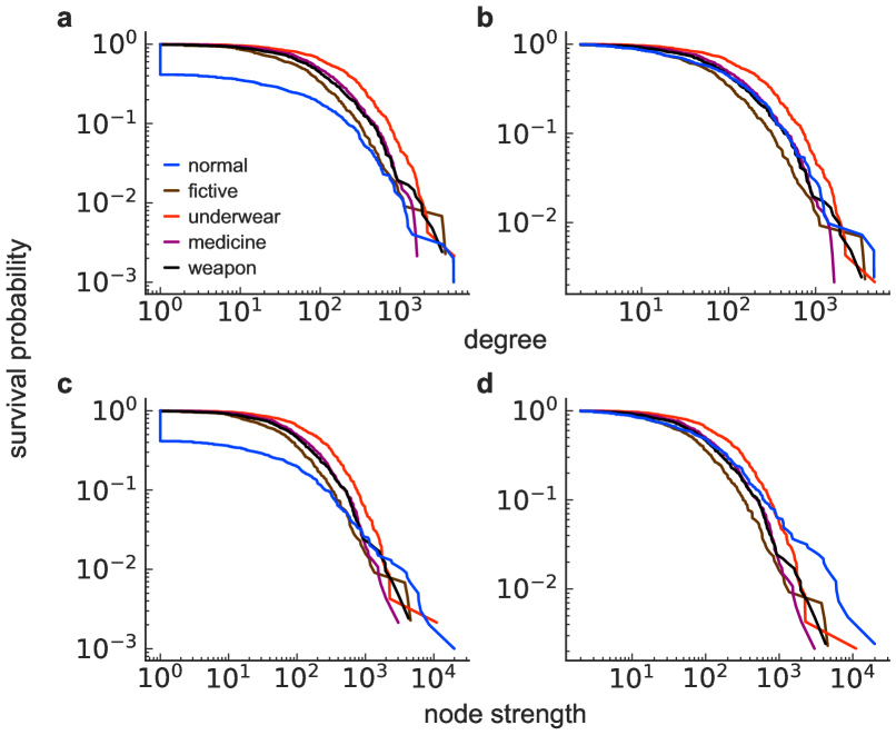
Figure 3: Survival probability of the degree for each user type. (a) Degree (i.e., $k_{i}$) for all nodes. (b) Degree for the nodes with $k_{i}\geq 2$. (c) Strength (i.e., $s_{i}$) for all nodes. (d) Strength for the nodes with $s_{i}\geq 2$.

The survival probability of the degree (i.e., a fraction of nodes whose degree is larger than a specified value) is shown in Fig. 3a for each user type. Approximately 60% of the normal users have degree $k_{i}=1$, whereas the fraction of the users with $k_{i}=1$ is approximately equal to 2% or less for any type of fraudulent user (Table 1). Therefore, we expect that whether $k_{i}=1$ or $k_{i}\geq 2$ gives useful information for distinguishing between normal and fraudulent users. The degree distribution at $k_{i}\geq 2$ may provide further information useful for the classification. The survival probability of the degree distribution conditioned on $k_{i}\geq 2$ for the different types of users is shown in Fig. 3b. The figure suggests that the degree distribution is systematically different between the normal and fraudulent users. However, we consider that the difference is not as clear-cut as that in the fraction of users having $k_{i}=1$ (Table 1).

Table 1: Properties of different types of users. In the first column, mean($\mathrm{A}\mid\mathrm{B}$), for example, represents the mean of A conditioned on B. Unless the first column mentions the conditional mean, median, or the number of transactions, the numbers reported in the table represent the number of users.

Seed user type	Normal	Fictive	Underwear	Medicine	Weapon
Number of seed users	999	440	468	469	416
Number of transactions involving the seed user	151,021	66,215	151,278	92,497	81,970
Total number of transactions	27,683,860	850,739	2,325,898	925,361	533,963
$k_{i}=1$	587 (58.8%)	8 (1.8%)	3 (0.6%)	2 (0.4%)	5 (1.2%)
mean($k_{i}\mid k_{i}\geq 2$)	195.0	138.3	297.8	184.2	179.7
median($k_{i}\mid k_{i}\geq 2$)	77.5	61.0	170.0	97.0	86.0
$s_{i}=1$	587 (58.8%)	8 (1.8%)	3 (0.6%)	2 (0.4%)	5 (1.2%)
mean($s_{i}\mid s_{i}\geq 2$)	365.1	153.3	325.3	198.1	199.4
median($s_{i}\mid s_{i}\geq 2$)	89.0	66.5	175.0	100.0	90.0
$s_{i}\geq 2$	412	432	465	467	411
$s_{i}/k_{i}=1$	97 (23.5%)	97 (22.5%)	86 (18.5%)	156 (33.4%)	121 (29.4%)
mean($s_{i}/k_{i}\mid s_{i}/k_{i}>1$)	1.413	1.135	1.055	1.066	1.092
median($s_{i}/k_{i}\mid s_{i}/k_{i}>1$)	1.124	1.059	1.03	1.031	1.055
$k_{i}\geq 2$	412	432	465	467	411
$\mathrm{SP}_{i}=1$	157 (38.1%)	15 (3.5%)	21 (4.5%)	16 (3.4%)	17 (4.1%)
$k_{i}^{\mathrm{out}}=1$	118 (28.6%)	21 (4.9%)	2 (0.4%)	2 (0.4%)	9 (2.2%)
$s_{i}\geq 2$	412	432	465	467	411
$\mathrm{WSP}_{i}=1$	157 (38.1%)	15 (3.5%)	21 (4.5%)	16 (3.4%)	17 (4.1%)
$s_{i}^{\mathrm{out}}=1$	118 (28.6%)	14 (3.2%)	2 (0.4%)	2 (0.4%)	9 (2.2%)
$k_{i}\geq 2$	412	432	465	467	411
$C_{i}=0$	118 (28.6%)	152 (35.2%)	108 (23.2%)	154 (33.0%)	128 (31.1%)
mean($C_{i}\mid C_{i}>0$)	$8.554\times 10^{-3}$	$8.348\times 10^{-3}$	$9.500\times 10^{-4}$	$2.231\times 10^{-3}$	$3.810\times 10^{-3}$
median($C_{i}\mid C_{i}>0$)	$2.411\times 10^{-3}$	$2.039\times 10^{-3}$	$5.288\times 10^{-4}$	$6.494\times 10^{-4}$	$1.337\times 10^{-3}$
$\mathrm{Tr}_{i}\geq 2$	262	241	317	251	244
$m_{i}=0$	17 (6.5%)	27 (11.2%)	54 (17.0%)	44 (17.5%)	32 (13.1%)
$m_{i}=1$	12 (4.6%)	9 (3.7%)	4 (1.3%)	6 (2.4%)	11 (4.5%)
mean($m_{i}\mid m_{i}>0$)	$8.554\times 10^{-3}$	$8.348\times 10^{-3}$	$9.500\times 10^{-4}$	$2.231\times 10^{-3}$	$3.810\times 10^{-3}$
median($m_{i}\mid m_{i}>0$)	$2.411\times 10^{-3}$	$2.039\times 10^{-3}$	$5.288\times 10^{-4}$	$6.494\times 10^{-4}$	$1.337\times 10^{-3}$
$\mathrm{FF}_{i}+\mathrm{CY}_{i}\geq 1$	294	280	357	313	283
$\mathrm{CYP}_{i}=0$	234 (79.6%)	188 (67.1%)	222 (62.2%)	227 (72.5%)	202 (71.4%)
mean($\mathrm{CYP}_{i}\mid\mathrm{CYP}_{i}>0$)	$1.987\times 10^{-2}$	$7.367\times 10^{-2}$	$6.739\times 10^{-2}$	$8.551\times 10^{-2}$	$5.544\times 10^{-2}$
median($\mathrm{CYP}_{i}\mid\mathrm{CYP}_{i}>0$)	$1.521\times 10^{-2}$	$4.481\times 10^{-2}$	$3.396\times 10^{-2}$	$3.822\times 10^{-2}$	$3.618\times 10^{-2}$

The survival probability of the node strength (i.e., weighted degree) is shown in Fig. 3c for each user type. As in the case for the unweighted degree, we found that many normal users, but not fraudulent users, have $s_{i}=1$. In fact, the number of the normal users with $s_{i}=1$ is equal to those with $k_{i}=1$ (Table 1), implying that all normal users with $k_{i}=1$ participated in just one transaction. In contrast, no user had $s_{i}=1$ for any type of fraudulent user. The survival probability of the node strength conditioned on $s_{i}\geq 2$ apparently does not show a clear distinction between the normal and fraudulent users (Fig. 3d, Table 1).

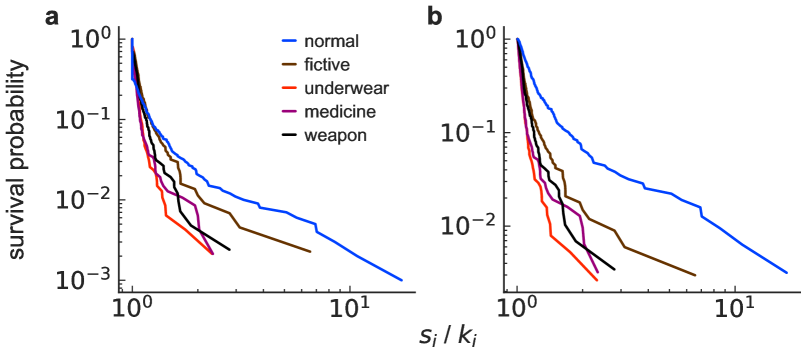
Figure 4: Survival probability of the average number of transactions per neighbor. (a) $s_{i}/k_{i}$ for all nodes. (b) $s_{i}/k_{i}$ for the nodes with $s_{i}/k_{i}>1$.

The distribution of the average number of transactions per edge, i.e., $s_{i}/k_{i}$, is shown in Fig. 4a. We found that a majority of normal users have $s_{i}/k_{i}=1$. This result indicates that a large fraction of normal users is engaged in just one transaction per neighbor (Table 1). This result is consistent with the fact that approximately 60% of the normal users have $k_{i}=s_{i}=1$. In contrast, many of any type of fraudulent users have $s_{i}/k_{i}>1$. However, they tend to have a smaller value of $s_{i}/k_{i}$ than the normal users. This difference is more noticeable when we discraded the users with $s_{i}/k_{i}=1$ (Fig. 4b, Table 1). Therefore, less frequent transactions with a specific neighbor seem to be a characteristic behavior of fraudulent users.

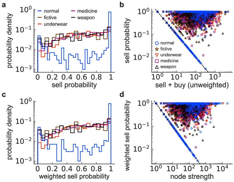
Figure 5: Sell probability for each user type. (a) Distribution of the unweighted sell probability. (b) Relationship between the degree and the unweighted sell probability. (c) Distribution of the weighted sell probability. (d) Relationship between the node strength and the weighted sell probability. The dashed lines in (b) and (d) indicate $1/(k_{i}^{\mathrm{in}}+k_{i}^{\mathrm{out}})$ and $1/(s_{i}^{\mathrm{in}}+s_{i}^{\mathrm{out}})$, respectively.

The distribution of the unweighted sell probability for the different user types is shown in Fig. 5a. The distribution for the normal users is peaked around 0 and 1, indicating that a relatively large fraction of normal users is almost exclusive buyer or seller. Note that, by definition, the sell probability is at least $1/(k_{i}^{\mathrm{in}}+k_{i}^{\mathrm{out}})$ because our samples are sellers. Therefore, a peak around the sell probability of zero implies that the users probably have no or few sell transactions apart from the one sell transaction based on which the users have been sampled as seller. In contrast, the distribution for any fraudulent type is relatively flat. Figure 5b shows the relationships between the unweighted sell probability and the degree. On the dashed line in Fig. 5b, the sell probability is equal to $1/(k_{i}^{\mathrm{in}}+k_{i}^{\mathrm{out}})$, indicating that the node has $k_{i}^{\mathrm{out}}=1$, which is the smallest possible out-degree. The users on this line were buyers in all but one transaction. Figure 5b indicates that a majority of such users are normal as opposed to fraudulent users, which is quantitatively confirmed in Table 1. We also found that most of the normal users were either on the horizontal line with the sell probability of one (38.1% of the normal users with $k_{i}\geq 2$; see Table 1 for the corresponding fractions of normal users with $k_{i}=1$) or on the dashed line (28.6%). This is not the case for any type of fraudulent user (Table 1).

The distribution of the weighted sell probability for the different user types and the relationships between the weighted sell probability and the node strength are shown in Fig. 5c and Fig. 5d, respectively. The results are similar to the case of the unweighted sell probability in two aspects. First, the normal users and the fraudulent users form distinct frequency distributions (Fig. 5c). Second, most of the normal users are either on the horizontal line with the weighted sell probability of one or on the dashed line with the smallest possible weighted sell probability, i.e., $1/s_{i}$ (Fig. 5d, Table 1).

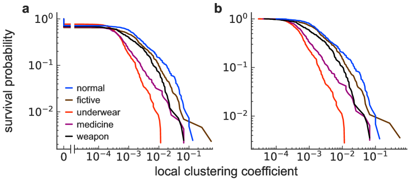
Figure 6: Local clustering coefficient for each user type. (a) Survival probability. (b) Survival probability conditioned on $C_{i}>0$.

The survival probability of the local clustering coefficient is shown in Fig. 6a. It should be noted that, in this analysis, we confined ourselves to the users with $k_{i}\geq 2$ because $C_{i}$ is undefined when $k_{i}=1$. We found that the number of users with $C_{i}=0$ is not considerably different between the normal and fraudulent users (also see Table 1). Figure 6b shows the survival probability of $C_{i}$ conditioned on $C_{i}>0$. The normal users tend to have a larger value of $C_{i}$ than fraudulent users, whereas this tendency is not strong (Table 1).

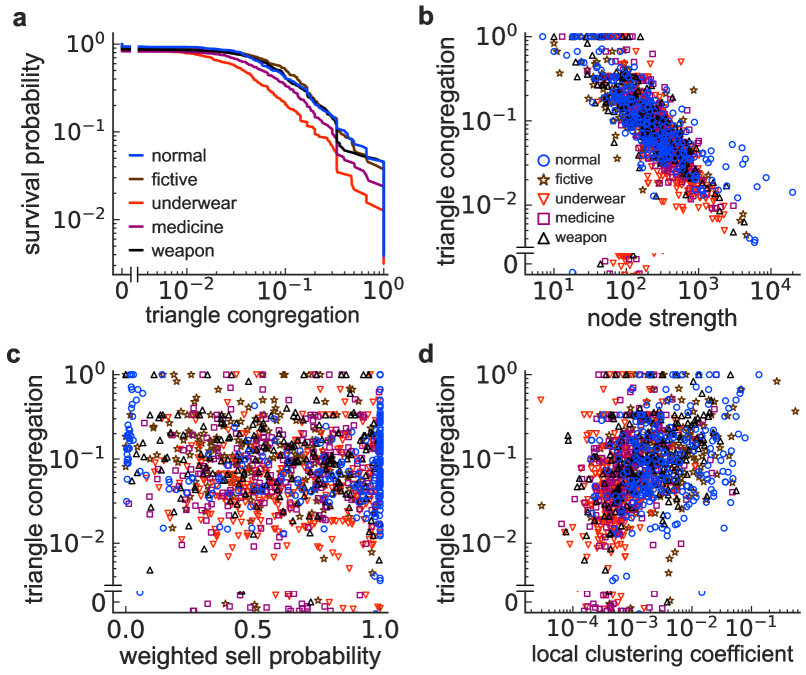
Figure 7: Triangle congregation for each user type. (a) Survival probability. (b) Relationship between the triangle congregation, $m_{i}$, and the node strength. (c) Relationship between $m_{i}$ and the weighted sell probability. (d) Relationship between $m_{i}$ and the local clustering coefficient.

The survival probability of the triangle congregation is shown in Fig. 7a. Contrary to our hypothesis, there is no clear difference between the distribution of the normal and fraudulent users. The triangle congregation tends to be large when the node strength is small (Fig. 7b) and the local clustering coefficient is large (Fig. 7d). It depends little on the weighted sell probability (Fig. 7c). However, we did not find clear differences in the triangle congregation between the normal and fraudulent users (also see Table 1).

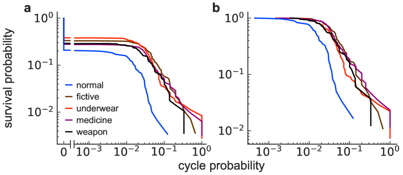
Figure 8: Cycle probability for each user type. (a) Survival probability. (b) Survival probability conditioned on CYP${}_{i}>0$.

The survival probability of the cycle probability is shown in Fig. 8a. A large fraction of any type of users has $\mathrm{CYP}_{i}=0$ (Table 1). When the users with $\mathrm{CYP}_{i}=0$ are discarded, the normal users tend to have a smaller value of $\mathrm{CYP}_{i}$ than any type of fraudulent users (Fig. 8b, Table 1).

Classification of users

Based on the eight indices whose descriptive statistics were analyzed in the previous section, we defined 12 features and fed them to the random forest classifier. The aim of the classifier is to distinguish between normal and fraudulent users. The first feature is binary and whether the degree $k_{i}=1$ or $k_{i}\geq 2$. The second feature is also binary and whether the node strength $s_{i}=1$ or $s_{i}\geq 2$. The third feature is $s_{i}/k_{i}$, which is a real number greater than or equal to 1. The fourth feature is binary and whether the unweighted sell probability $\mathrm{SP}_{i}=1$ or $\mathrm{SP}_{i}<1$. The fifth feature is binary and whether $\mathrm{SP}_{i}=1/(k_{i}^{\mathrm{in}}+k_{i}^{\mathrm{out}})$ or $\mathrm{SP}_{i}>1/(k_{i}^{\mathrm{in}}+k_{i}^{\mathrm{out}})$, i.e., whether $k_{i}^{\mathrm{out}}=1$ or $k_{i}^{\mathrm{out}}>1$. The sixth feature is $\mathrm{SP}_{i}$, which ranges between 0 and 1. The seventh feature is binary and whether the weighted sell probability $\mathrm{WSP}_{i}=1$ or $\mathrm{WSP}_{i}<1$. The eighth feature is binary and whether $\mathrm{WSP}_{i}=1/(s_{i}^{\mathrm{in}}+s_{i}^{\mathrm{out}})$ or $\mathrm{WSP}_{i}>1/(s_{i}^{\mathrm{in}}+s_{i}^{\mathrm{out}})$, i.e., whether $s_{i}^{\mathrm{out}}=1$ or $s_{i}^{\mathrm{out}}>1$. The ninth feature is $\mathrm{WSP}_{i}$, which ranges between 0 and 1. The tenth feature is the local clustering coefficient $C_{i}$, which ranges between 0 and 1. When $k_{i}=1$, the local clustering coefficient is undefined. In this case, we set $C_{i}=-1$. The eleventh feature is the triangle congregation $m_{i}$, which ranges between 0 and 1. When there is no triangle or only one triangle involving $v_{i}$, one cannot calculate $m_{i}$. In this case, we set $m_{i}=-1$. Finally, the twelfth feature is the cycle probability $\mathrm{CYP}_{i}$, which ranges between 0 and 1. When there is neither feedforward nor cyclic triangle involving $v_{i}$, $\mathrm{CYP}_{i}$ is undefined. In this case, we set $\mathrm{CYP}_{i}=-1$.

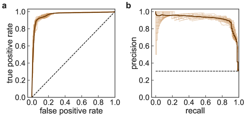
Figure 9: ROC and PR curves when the normal users and those involved in fictive transactions are classified. (a) ROC curves. (b) PR curves. Each thin line corresponds to one of the 100 classifiers. The thick lines correspond to the average of the 100 lines. The dashed lines correspond to the uniformly random classification.

The ROC and PR curves when all the 12 features of users are used and the fraudulent type is fictive transactions are shown in Figs. 9a and b, respectively. Each thin line corresponds to one of the 100 classifiers. The thick lines correspond to the average of the 100 lines. The dashed lines correspond to the uniformly random classification. Figure 9 indicates that the classification performance seems to be high. Quantitatively, for this and the other types of fraudulent users, the AUC values always exceeded 0.91 (Table 2).

Table 2: AUC values for the random forest classifiers. The average and standard deviation were calculated based on the 100 classifiers.

		Fictive	Underwear	Medicine	Weapon
12 features	ROC	0.962 $\pm$ 0.003	0.981 $\pm$ 0.001	0.979 $\pm$ 0.003	0.969 $\pm$ 0.004
	PR	0.916 $\pm$ 0.009	0.948 $\pm$ 0.006	0.947 $\pm$ 0.005	0.916 $\pm$ 0.015
9 features	ROC	0.951 $\pm$ 0.003	0.973 $\pm$ 0.003	0.971 $\pm$ 0.003	0.961 $\pm$ 0.004
	PR	0.889 $\pm$ 0.009	0.923 $\pm$ 0.010	0.930 $\pm$ 0.009	0.888 $\pm$ 0.025

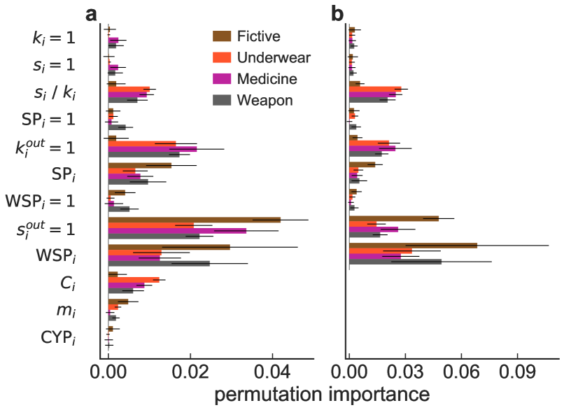
Figure 10: Permutation importance of the features in the random forest classifier. (a) 12 features. (b) 9 features. The bars indicate the average over the 100 classifiers. The error bars indicate standard deviation.

The importance of each feature in the classifier is shown in Fig. 10a, separately for the different fraud types. The importance of each feature is similar across the different types of fraud. Figure 10a indicates that the average number of transactions per neighbor (i.e., $s_{i}/k_{i}$), whether or not $k_{i}^{\mathrm{out}}=1$ (i.e., SP${}_{i}=1/(k_{i}^{\mathrm{in}}+k_{i}^{\mathrm{out}})$), whether or not $s_{i}^{\mathrm{out}}=1$ (i.e., WSP${}_{i}=1/(s_{i}^{\mathrm{in}}+s_{i}^{\mathrm{out}})$), and the weighted sell probability (i.e., WSP_i) are the four features of the highest importance. Given the results of the descriptive statistics in the previous section, a small value of $s_{i}/k_{i}$, $k_{i}^{\mathrm{out}}\neq 1$, $s_{i}^{\mathrm{out}}\neq 1$, and a moderate WSP_i value strongly suggest that the user may be fraudulent.

Figure 10a also suggests that the features based on the triangles, i.e., $C_{i}$, $m_{i}$, and $\mathrm{CYP}_{i}$, are not strong contributors to the classifier’s performance. Because these features are the only ones that require the information about the connectivity between pairs of neighbors of the focal node, it is practically beneficial if one can realize a similar classification performance without using these features; then only the information on the connectivity of the focal users is required. To explore this possibility, we constructed the random forest classifier using the nine out of the twelve features that do not require the connectivity between neighbors of the focal node. The mean AUC values for the ROC and PR curves are shown in Table 2. We find that, despite some reduction in the performance scores relative to the case of the classifier using all the 12 features, the AUC values with the nine features are still large, all exceeding 0.88. The permutation importance of the nine features is shown in Fig. 10b. The results are similar to those when all the 12 features are used, although the importance of WSP_i considerably increased in the case of the nine features (Fig. 10a).

More than half of the normal users have $k_{i}=1$, and there are few fraudulent users with $k_{i}=1$ in each fraud category (Table 1). The classification between the normal and fraudulent users may be an easy problem for this reason, leading to the large AUC values. To exclude this possibility, we carried out a classification test for the subdata in which the normal and fraudulent users with $k_{i}=1$ were excluded, leaving 412 normal users and a similar number of fraudulent users in each category (Table 1). We did not carry out subsampling because the number of the negative and positive samples were similar. Instead, we generated 100 different sets of train and test samples and built a classifier based on each set of train and test samples. The AUC values when either 10 or 7 features (i.e., the features excluding whether or not $k_{i}=1$ and whether or not $s_{i}=1$) are used are shown in Table 3. The table indicates that the AUC values are still competitively large while they are smaller than those when whether or not $k_{i}=1$ and whether or not $s_{i}=1$ are used as features (Table 2).

Table 3: AUC values for the random forest classifiers excluding users with $k_{i}=1$. The average and standard deviation were calculated based on the 100 classifiers.

		Fictive	Underwear	Medicine	Weapon
10 features	ROC	0.925 $\pm$ 0.016	0.950 $\pm$ 0.013	0.954 $\pm$ 0.012	0.916 $\pm$ 0.019
	PR	0.923 $\pm$ 0.019	0.950 $\pm$ 0.018	0.954 $\pm$ 0.016	0.911 $\pm$ 0.023
7 features	ROC	0.886 $\pm$ 0.020	0.921 $\pm$ 0.015	0.933 $\pm$ 0.014	0.899 $\pm$ 0.020
	PR	0.874 $\pm$ 0.027	0.901 $\pm$ 0.021	0.928 $\pm$ 0.019	0.880 $\pm$ 0.028

Discussion

We showed that a random forest classifier using network features of users distinguished different types of fraudulent users from normal users with approximately 0.91–0.98 in terms of the AUC. We only used the information about local transaction networks centered around focal users to synthesize their features. We did so because it is better in practice not to demand the information about global transaction networks due to the large number of users. It should be noted that AUC values of $\approx 0.88$–0.97 was also realized when we only used the information about the connectivity of the focal user, not the connectivity between the neighbors of the focal user. This result has a practical advantage when the present fraud-detection method is implemented online because it allows one to classify users with a smaller amount of data per user.

The random forest classifier is an arbitrary choice. One can alternatively use a different linear or nonlinear classifier to pursue a higher classification performance. This is left as future work. Other future tasks include the generalizability of the present results to different types of fraudulent transactions, such as resale tickets, pornography, and stolen items, and to different platforms. In particular, if a classifier trained with test samples from fraudulent users of a particular type and normal users is effective at detecting different types of fraud, the classifier will also be potentially useful for detecting unknown types of fraudulent transactions. It is also a potentially relevant question to assess the classification performance when one pools different types of fraud as a single positive category to train a classifier.

Prior network-based fraud detection has employed either global or local network properties to characterize nodes. Global network properties refer to those that require the structure of the entire network for calculating a quantity for individual nodes, such as the connected component [14, 17, 29], betweenness centrality[14, 15, 16], user’s suspiciousness determined by belief propagation [30, 31, 27, 33, 35, 20, 21, 36], dense subgraphs including the case of communities [14, 23, 22, 24, 25, 18, 19], and $k$-core[32, 26]. Although many of these methods have accrued a high classification performance, they require the information about the entire network. Obtaining such data may be difficult when the network is large or rapidly evolving over time, thus potentially compromising the computation speed, memory requirement, and the accuracy of the information on the nodes and edges. Alternatively, other methods employed local network properties such as the degree including the case of directed and/or weighted networks [30, 38, 14, 34, 23, 33, 15, 37, 20, 16] and the abundance of triangles and quadrangles [37, 20]. The use of local network properties may be advantageous in industrial contexts, particularly to test sampled users, because local quantities can be rapidly calculated given a seed node. Another reason for which we focused on local properties was that we could not obtain the global network structure for computational reasons. It should be noted that, while the use of global network properties in addition to local ones may improve the classification accuracy [23], the present local method attained a similar classification performance to those based on global network properties, i.e., 0.880–0.986 in terms of the ROC AUC [14, 35, 20, 21, 36, 17].

A prior study using data from the same marketplace, Mercari, aimed to distinguish between desirable non-professional frequent sellers and undesirable professional sellers[51]. The authors used information about user profiles, item descriptions, and other behavioral data such as the number of purchases per day. In contrast, we focused on local network features of the users (while a quantity similar to WSP_i was used as a feature in Ref.[51]). In addition, we used specific types of fraudulent transactions, whereas the authors of Ref.[51] focused on problematic transactions as a single broad category. How the present results generalize to different categorizations of fraudulent transactions, the platform’s different data such as their US market data, and similar data obtained from other online marketplaces is unknown. Combining network and non-network features may realize a better classification performance . Furthermore, using the information about the time of the transactions may also yield better classification. Using the time information allows us to ask new questions such as prediction of users’ behavior. These topics warrant future work.

Declarations

Abbreviations

C2C: consumer-to-consumer; ROC: receiver operating characteristic; PR: precision-recall; AUC: area under the curve

Ethics

Mercari, Inc. approved the use of the data for the present study under the condition that the data were hashed and only released to the collaborators of the project (i.e., the first and last authors, because the second and third authors are employees of the company).

Availability of data and materials

Mercari, Inc. approved the use of the data for the present study under the condition that the data were hashed and only released to the collaborators of the project (i.e., the first and last authors, because the second and third authors are employees of the company). The figures and tables of the present paper are summary statistics of the data and not sufficient on their own for others to replicate the results of the present study. Although the data have been hashed, the company cannot share the data with the public. This is because, if anybody traces the transaction data on the Mercari’s web platform and checks them against the hashed data, that person would be able to identify individual users including their private information. Therefore, hashing/anonymizing does not help to guarantee the users’ privacy. Any bona fide researcher could approach the company (Shunya Kimura: kimuras@mercari.com and Ryusuke Chiba: metalunk@mercari.com) to seek access to the complete dataset. However, for the aforementioned reasons, such an attempt is unlikely to be successful.

The users were made aware that their data may be used for the present research because the Mercari’s terms of use (in Japanese only: https://www.mercari.com/jp/tos/), Article 20, Term 2, states that their data can be used for research by the company and by those who the company permits.

Competing interests

The second and third authors are employees of the company that provided the data analysed in the present manuscript. However, this fact does not cause any conflict of interest because the analyses, results and their interpretation are free of any bias towards the merit of the company.

Funding

The authors acknowledge financial support by Mercari, Inc. S. Kodate was supported in part by the Top Global University Project from the Ministry of Education, Culture, Sports, Science and Technology (MEXT) of Japan.

Authors’ contributions

S. Kodate analyzed data, developed methodology, visualized the results, and drafted the manuscript; RC curated data and critically revised the manuscript; S. Kimura coordinated the study, acquired funding, and critically revised the manuscript; NM coordinated the study, acquired funding, developed methodology, drafted the manuscript. All authors gave final approval for publication and agreed to be held accountable for the work performed therein.

Acknowledgments

This work was carried out using the computational facilities of the Advanced Computing Research Centre, University of Bristol.

References

- 1. UK Parliament: The Growing Threat of Online Fraud. https://old.parliament.uk/business/committees/committees-a-z/commons-select/public-accounts-committee/inquiries/parliament-2017/growing-threat-online-fraud-17-19/publications/ (2017 (Accessed: November 1, 2020))
- 2. McAfee, LLC: Economic Impact of Cybercrime Report. https://www.mcafee.com/enterprise/en-us/solutions/lp/economics-cybercrime.html (2018 (Accessed: April 25, 2019))
- 3. Anderson, R., Barton, C., Böhme, R., Clayton, R., Van Eeten, M.J., Levi, M., Moore, T., Savage, S.: Measuring the cost of cybercrime. In: The Economics of Information Security and Privacy, pp. 265–300. Springer, Berlin, Heidelberg (2013)
- 4. Bolton, R.J., Hand, D.J.: Statistical fraud detection: A review. Statistical Science 17, 235–249 (2002)
- 5. Phua, C., Lee, V., Smith, K., Gayler, R.: A comprehensive survey of data mining-based fraud detection research. Preprint arXiv:1009.6119 (2010)
- 6. Abdallah, A., Maarof, M.A., Zainal, A.: Fraud detection system: A survey. J. Netw. Comput. Appl. 68, 90–113 (2016)
- 7. West, J., Bhattacharya, M.: Intelligent financial fraud detection: A comprehensive review. Computers & Security 57, 47–66 (2016)
- 8. Akoglu, L., Tong, H., Koutra, D.: Graph based anomaly detection and description: a survey. Data Min. Knowl. Discov. 29, 626–688 (2015)
- 9. Google LLC and White Ops, Inc: The Hunt for 3ve. https://services.google.com/fh/files/blogs/3ve_google_whiteops_whitepaper_final_nov_2018.pdf (2018 (Accessed: May 10, 2019))
- 10. Pu, C., Webb, S.: Observed trends in spam construction techniques: A case study of spam evolution. In: CEAS, pp. 104–112 (2006)
- 11. Hayes, B.: How many ways can you spell v1@gra? Amer. Sci. 95, 298–302 (2007)
- 12. Bhowmick, A., Hazarika, S.M.: Machine learning for e-mail spam filtering: review, techniques and trends. Preprint arXiv:1606.01042 (2016)
- 13. Savage, D., Zhang, X., Yu, X., Chou, P., Wang, Q.: Anomaly detection in online social networks. Soc. Netw. 39, 62–70 (2014)
- 14. Šubelj, L., Furlan, Š., Bajec, M.: An expert system for detecting automobile insurance fraud using social network analysis. Expert Syst. Appl. 38, 1039–1052 (2011)
- 15. Dreżewski, R., Sepielak, J., Filipkowski, W.: The application of social network analysis algorithms in a system supporting money laundering detection. Info. Sci. 295, 18–32 (2015)
- 16. Colladon, A.F., Remondi, E.: Using social network analysis to prevent money laundering. Expert Syst. Appl. 67, 49–58 (2017)
- 17. Savage, D., Wang, Q., Zhang, X., Chou, P., Yu, X.: Detection of money laundering groups: Supervised learning on small networks. In: Workshops at the Thirty-First AAAI Conference on Artificial Intelligence, pp. 43–49 (2017)
- 18. Liu, J., Bier, E., Wilson, A., Guerra-Gomez, J.A., Honda, T., Sricharan, K., Gilpin, L., Davies, D.: Graph analysis for detecting fraud, waste, and abuse in healthcare data. AI Magazine 37, 33–46 (2016)
- 19. Shchur, O., Bojchevski, A., Farghal, M., Günnemann, S., Saber, Y.: Anomaly detection in car-booking graphs. In: 2018 IEEE International Conference on Data Mining Workshops (ICDMW), pp. 604–607 (2018)
- 20. Van Vlasselaer, V., Eliassi-Rad, T., Akoglu, L., Snoeck, M., Baesens, B.: Gotcha! network-based fraud detection for social security fraud. Manag. Sci. 63, 3090–3110 (2016)
- 21. Hu, J., Liang, J., Dong, S.: ibgp: A bipartite graph propagation approach for mobile advertising fraud detection. Mobile Info. Syst. 2017, 1–12 (2017)
- 22. Ferrara, E., De Meo, P., Catanese, S., Fiumara, G.: Detecting criminal organizations in mobile phone networks. Expert Syst. Appl. 41, 5733–5750 (2014)
- 23. Bhat, S.Y., Abulaish, M.: Community-based features for identifying spammers in online social networks. In: 2013 IEEE/ACM International Conference on Advances in Social Networks Analysis and Mining (ASONAM 2013), pp. 100–107 (2013)
- 24. Jiang, M., Cui, P., Beutel, A., Faloutsos, C., Yang, S.: Inferring strange behavior from connectivity pattern in social networks. In: Pacific-Asia Conference on Knowledge Discovery and Data Mining, pp. 126–138 (2014)
- 25. Hooi, B., Song, H.A., Beutel, A., Shah, N., Shin, K., Faloutsos, C.: Fraudar: Bounding graph fraud in the face of camouflage. In: Proceedings of the 22nd ACM SIGKDD International Conference on Knowledge Discovery and Data Mining, pp. 895–904 (2016)
- 26. Rasheed, J., Akram, U., Malik, A.K.: Terrorist network analysis and identification of main actors using machine learning techniques. In: Proceedings of the 6th International Conference on Information Technology: IoT and Smart City, pp. 7–12 (2018)
- 27. Akoglu, L., Chandy, R., Faloutsos, C.: Opinion fraud detection in online reviews by network effects. In: Seventh International AAAI Conference on Weblogs and Social Media, pp. 2–11 (2013)
- 28. Liu, S., Hooi, B., Faloutsos, C.: Holoscope: Topology-and-spike aware fraud detection. In: Proceedings of the 2017 ACM on Conference on Information and Knowledge Management, pp. 1539–1548 (2017)
- 29. Wang, Z., Gu, S., Zhao, X., Xu, X.: Graph-based review spammer group detection. Knowl. Info. Syst. 55, 571–597 (2018)
- 30. Chau, D.H., Pandit, S., Faloutsos, C.: Detecting fraudulent personalities in networks of online auctioneers. In: European Conference on Principles of Data Mining and Knowledge Discovery, pp. 103–114 (2006)
- 31. Pandit, S., Chau, D.H., Wang, S., Faloutsos, C.: Netprobe: A fast and scalable system for fraud detection in online auction networks. In: Proceedings of the 16th International Conference on World Wide Web, pp. 201–210 (2007)
- 32. Wang, J.-C., Chiu, C.-C.: Recommending trusted online auction sellers using social network analysis. Expert Syst. Appl. 34, 1666–1679 (2008)
- 33. Bangcharoensap, P., Kobayashi, H., Shimizu, N., Yamauchi, S., Murata, T.: Two step graph-based semi-supervised learning for online auction fraud detection. In: Joint European Conference on Machine Learning and Knowledge Discovery in Databases, pp. 165–179 (2015)
- 34. Yanchun, Z., Wei, Z., Changhai, Y.: Detection of feedback reputation fraud in taobao using social network theory. In: 2011 International Joint Conference on Service Sciences, pp. 188–192 (2011)
- 35. Van Vlasselaer, V., Bravo, C., Caelen, O., Eliassi-Rad, T., Akoglu, L., Snoeck, M., Baesens, B.: Apate: A novel approach for automated credit card transaction fraud detection using network-based extensions. Decision Support Syst. 75, 38–48 (2015)
- 36. Li, Y., Sun, Y., Contractor, N.: Graph mining assisted semi-supervised learning for fraudulent cash-out detection. In: Proceedings of the 2017 IEEE/ACM International Conference on Advances in Social Networks Analysis and Mining 2017, pp. 546–553 (2017)
- 37. Monamo, P., Marivate, V., Twala, B.: Unsupervised learning for robust bitcoin fraud detection. In: 2016 Information Security for South Africa (ISSA), pp. 129–134 (2016)
- 38. Akoglu, L., McGlohon, M., Faloutsos, C.: Oddball: Spotting anomalies in weighted graphs. In: Pacific-Asia Conference on Knowledge Discovery and Data Mining, pp. 410–421 (2010)
- 39. Mercari, Inc: FY2019.6 Q3 Presentation Material. https://about.mercari.com/en/ir/library/results/ ((Accessed: November 1, 2020))
- 40. Barrat, A., Barthelemy, M., Pastor-Satorras, R., Vespignani, A.: The architecture of complex weighted networks. Proc. Natl. Acad. Sci. USA 101, 3747–3752 (2004)
- 41. Newman, M.: Networks: An Introduction. Oxford University Press, Oxford (2010)
- 42. Radicchi, F., Castellano, C., Cecconi, F., Loreto, V., Parisi, D.: Defining and identifying communities in networks. Proc. Natl. Acad. Sci. USA 101, 2658–2663 (2004)
- 43. Palla, G., Derényi, I., Farkas, I., Vicsek, T.: Uncovering the overlapping community structure of complex networks in nature and society. Nature 435, 814–818 (2005)
- 44. Milo, R., Shen-Orr, S., Itzkovitz, S., Kashtan, N., Chklovskii, D., Alon, U.: Network motifs: Simple building blocks of complex networks. Science 298, 824–827 (2002)
- 45. Breiman, L.: Random forests. Machine Learning 45, 5–32 (2001)
- 46. Breiman, L., Friedman, J.H., Olshen, R.A., Stone, C.J.: Classification and Regression Trees. Chapman & Hall/CRC, Boca Raton, FL (1984)
- 47. Hastie, T., Tibshirani, R., Friedman, J.: The Elements of Statistical Learning: Data Mining, Inference, and Prediction. Springer, New York, NY (2009)
- 48. Pedregosa, F., Varoquaux, G., Gramfort, A., Michel, V., Thirion, B., Grisel, O., Blondel, M., Prettenhofer, P., Weiss, R., Dubourg, V., et al.: Scikit-learn: Machine learning in python. J. Machine Learning Res. 12, 2825–2830 (2011)
- 49. Strobl, C., Boulesteix, A.-L., Zeileis, A., Hothorn, T.: Bias in random forest variable importance measures: Illustrations, sources and a solution. BMC bioinformatics 8, 25 (2007)
- 50. Altmann, A., Toloşi, L., Sander, O., Lengauer, T.: Permutation importance: A corrected feature importance measure. Bioinformatics 26, 1340–1347 (2010)
- 51. Yamamoto, H., Sugiyama, N., Toriumi, F., Kashida, H., Yamaguchi, T.: Angels or demons? classifying desirable heavy users and undesirable power sellers in online c2c marketplace. J Comput Soc Sc 2, 315–329 (2019)