How to avoid X’es around point sources in maximum likelihood CMB maps

Abstract

The maximum likelihood estimator for CMB map-making is optimal and unbiased as long as the data model is correct, but in practice it rarely is, with model errors including sub-pixel structure and instrumental problems like time-variable gain and pointing errors. In the presence of such errors, the solution is biased, with the local error in each pixel leaking outwards along the scanning pattern by a noise correlation length. The most important sources of such leakage are strong point sources, and for common scanning patterns the leakage manifests as an X around each such source. I discuss why this happens, and present several old and new methods for mitigating and/or eliminating this leakage, along with a small stand-alone TOD simulator and map-maker in Python that implements them.

1 Introduction

Cosmic Microwave Background (CMB) telescopes map the sky by scanning an array of detectors repeatedly across the sky, resulting in a time-series of samples $d$. This process is usually modeled via the linear equation (Tegmark, 1997)

$$d =Pm+n$$ (1)

where $d$ is the vector of samples, $m$ is a vector representing the pixels of the sky we are trying to reconstruct, and $P$ is a response matrix that encodes where the telescope was pointing on the sky when each sample was taken and how it responded to that. $n$ represents the noise contribution to each sample, and is usually taken to be normal distributed with some covariance $N$. The maximum likelihood solution to this equation is

$$\hat{m} =(P^{T}N^{-1}P)^{-1}P^{T}N^{-1}d\equiv M_{PN}d$$ (2)

where $M_{N}$ is the map-making operator using the response matrix $P$ and the noise model $N$. It’s simple to see that this solution is unbiased by inserting our model for $d$:

$$\langle\hat{m}\rangle =(P^{T}N^{-1}P)^{-1}P^{T}N^{-1}(Pm+\overbrace{\langle n\rangle}^{0})=m$$ (3)

Given this result it might be surprising to hear that most maximum-likelihood maps made using eq. 2 are biased to some extent, with the archetypical example being linear artifacts extending away from bright point sources in the map, often in the shape of an X (but this depends on the telescope’s scanning pattern). The source of these artifacts is model error: the failure of eq. 1 to accurately describe the real data; and in this paper I will describe the main types of model error in maximum-likelihood mapmaking, simulate their effect and investigate several old and new methods for mitigating or eliminating them.

2 Sources of model error

2.1 Sub-pixel structure

The most obvious problem with eq. 1 is that it models the sky as a finite vector of pixels, which will leave out any signal on scales smaller than the pixel spacing. This is exacerbated by the canonical choice of a nearest-neighbor response model in $P$. Every CMB map-maker I am aware of uses nearest-neighbor, including destripers like MADAM (Keihänen et al., 2010) and SRoll (Planck Collaboration, 2018), filter+bin map-makers like those used in SPT (Schaffer et al., 2011) and BICEP (BICEP2 Collaboration, 2014) or the maximum likelihood map-makers used in ACT (ACT Collaboration, 2017) and QUIET (Ruud et al., 2015). In this model, the value of each sample is simply given by the value of the closest pixel to it, regardless of how far away from the pixel center it is. This results in a response matrix with a very simple structure: For each row (representing a sample) a single element will be 1 (representing the pixel hit by that sample), and all others will be zero.

Multiplication by a matrix with this structure is simple and efficient. Given a map m[ny,nx] and arrays y[nsamp], x[nsamp] containing the x and y pixel coordinates of each sample, the forward operation $d=Pm$ can be implemented as

⬇

for i in range(nsamp):

d[i] = m[round(y[i]),round(x[i])]

and the transpose operation $m=P^{T}d$ can be implemented as

⬇

for i in range(nsamp):

m[round(y[i]),round(x[i])] += d[i]

However, this simplicity comes at a cost: The signal model implied by this response matrix has a constant value inside each pixel and a discontinuous jump at the edge of each pixel. This model and the resulting error is illustrated in figure 1.

uncorrelated	correlated

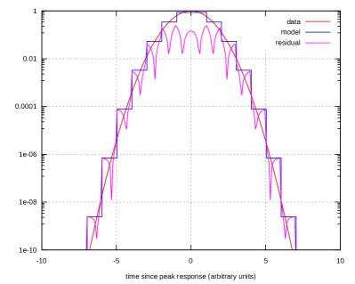
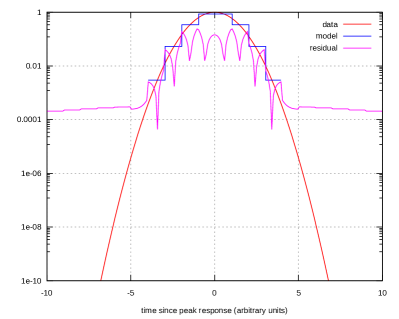
Figure 1: A simulated data vector consisting of a noiseless scan through a smooth, Gaussian profile, compared to its nearest-neighbor-pixellated maximum likelihood model. Left: When an uncorrelated noise model is used ($N\propto I$) the residual is large but stays in the pixel where they were sourced. This error can be characterized as a simple pixel window. Right: When a correlated noise model is used the residuals are still large, but are now spread out over a larger area than the signal that sourced them.

A step-function model like this clearly cannot match the smooth behavior of the beam-convolved sky, and the only term in eq. 1 that can absorb such a mismatch between the data and the model is the noise term $n$. How this model error manifests is therefore determined by our noise model $N$.

If $N$ is assumed to be uncorrelated ($N$ diagonal in time domain), then a high value of the residual (honorary noise as far as our data model is concerned) in one sample does not tell us anything about what the noise is doing in any other samples, and so the residual just stays in the pixel that birthed it. The value in each pixel is therefore just the mean of the samples that hit it (left panel of figure 1). This is approximately the mean value of the signal inside the area covered by the pixel, which is a straightforward and useful thing to measure, and is not the sort of bias we are worried about here.

If, on the other hand, $N$ is assumed to be correlated, then the presence of high “noise” (actually residual) in some samples will make the maximum likelihood prection for other samples within a noise correlation length have a similar value for the noise. For long correlation lengths this could affect samples many pixels away from the source of the residual. This is illustrated in the right panel of figure 1. Here large sub-pixel residuals in the center result in a non-zero expectation value for the noise at large distances. Given that the actual data has negligibly small values there, the best fit model must cancel the expected noise, resulting in a non-zero model extending far beyond the area with significant signal. Effectively the correlated noise model is causing local model errors to leak roughly a correlation length into the surrounding pixels.

2.2 Signal or instrumental variability

Real telescopes don’t have 100% accurate pointing and gain, and even if they did, the sky is not static and unchanging. These effects mean the telescope effectively sees the sky jitter around slightly while varying in brightness. There is no room for this in eq. 1 aside from the noise term $n$, so time-variable instrumental errors or variable point sources will lead to exactly the same sort of artifacts as sub-pixel errors do.

3 Mitigation methods

The artifacts are ultimately caused by a combination of two factors:

1. Multiple samples are mapped onto the same pixel, but don’t agree on what the signal in that pixel should be.

2. The correlated noise model causes a non-local response to such errors.

This points to two approaches for eliminating them: Improve the model so it matches the data more accurately, or modify the noise model to make it more local.

3.1 Higher-order mapmaking

An obvious way to improve the model is to replace nearest-neibhor interpolation in the response matrix $P$ with smoother interpolation functions such as bilinear or bicubic spline interpolation. These are popular in image processing, but are as far as I am aware unused in CMB map making.

Bilinear interpolation is considerably slower and more complicated than nearest neighbor, and each sample now interacts with the four closest pixels instead of just one. The forward operation $d=Pm$ is now (based on the implementaiton of scipy.ndimage.map_coordinates):

⬇

for i in range(nsamp):

py1, px1 = floor(y[i]), floor(x[i])

py2, px1 = py1+2, px1+1

ry, rx = y[i]-py1, x[i]-px1

vx1 = m[py1,px1] * (1-rx) + m[py1,px2] * rx

vx2 = m[py2,px1] * (1-rx) + m[py2,px2] * rx

d[i] = vx1 * (1-ry) + vx2 * ry

The transpose operation $m=P^{T}d$ is:

⬇

for i in range(nsamp):

py1, px1 = floor(y[i]), floor(x[i])

py2, px1 = py1+2, px1+1

ry, rx = y[i]-py1, x[i]-px1

vx1 = d[i] * (1-ry)

vx2 = d[i] * ry

m[py1,px1] += vx1 * (1-rx)

m[py1,px2] += vx1 * rx

m[py2,px1] += vx2 * (1-rx)

m[py2,px2] += vx2 * rx

Bicubic spline interpolation is another large step up in complexity. See the appendix for details.

Figure 2 shows how these higher-order interpolation schemes perform for the same 1D Gaussian simulation we considered in figure 1

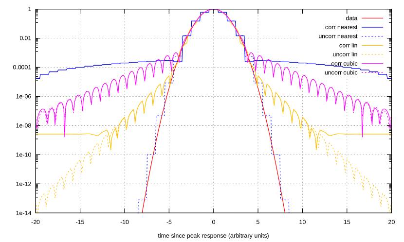
Figure 2: Comparison of the maximum-likelihood models for nearest neighbor, linear and cubic interpolation in the response matrix for uncorrelated and correlated noise models, for the same data as in figure 1. Linear and cubic interpolation fit the central part of the profile much better than nearest neighbor, leading to lower discrepancy between the data and model at high radius in the correlated case (solid curves). But this situation is reversed for the uncorrelated noise model (dashed curves). This happens because the linear and cubic models are inherently non-local, and are willing to sacrifice accuracy in areas where the signal is very weak in order to get a better match in areas with strong signal.

Both linear and cubic interpolation fit the peak of the Gaussian much better than nearest neighbor, resulting in roughly 4 orders of magnitude lower spurious signal at high radius for the case with a correlated noise model. However, they only reach this level at large radii. Before this, the spurious signal is dominated by a new effect that was not present for nearest neighbor interpolation: Higher order interpolation is inherently non-local, which means that each pixel is correlated with its neighbors (and neighbors-neighbors for bicubic). This is responsible for the exponentially decaying ringing pattern we see in the figure for these interpolation types, even for uncorrelated noise. Effectively the fit is sacrificing accuracy at large radius in order to fit the strong, central peak slightly better.

So we see that high interpolation order has smaller total residuals and hence lower non-local artifacts from the noise correlations, but low-order interpolation has shorter correlation length for the interpolation functions themselves, leading to a faster decay of the ringing. For the example in figure 2, the sweet spot is linear interpolation. Even better locality (at even higher cost) should be possible with an interpolation function based on the actual point spread function of the instrument.

Aside from the high cost and non-locality inherent in these interpolators, they are also limited by only addressing sub-pixel errors. Higher-order map-making does nothing to remove artifacts from variable instrumental errors or intrinsic sky variability.

3.1.1 Iterative approximation

Since the response matrix often is the bottleneck in maximum-likelihood mapmaking, it may be too expensive to make this step several times slower by using higher-order mapmaking. A simple approximation that avoids most of this slowdown is to first make a normal map using the fast, nearest-neighbor response matrix, and then subtract this estimate of the sky from the time-ordered data using a bilinear or bicubic spline response matrix. This process can be repeated if necessary, though in my tests there was little point in doing more than 1-3 iterations.

$$\hat{m}_{0} =0$$

$$\hat{m}_{i+1} =\hat{m}_{i}+M_{PN}(d-\bar{P}\hat{m}_{i})$$ (4)

Here $P$ is the standard nearest-neighbor response matrix and $\bar{P}$ is the higher-order one we are approximating. Note that this iteration converges on an approximation to the higher-order map, not the exact solution we would have gotten by using $\bar{P}$ in the equation 2. However, as we shall see in the results section it does a pretty good job.

If one is already doing iterative mapmaking to avoid bias from estimating the noise model $N$ from the full data $d$ rather than just the noise $n$, then this iterative approximation to higher-order mapmaking can simply be done as a part of that, and will incur almost no extra cost.

Alternatively, if one is solving for each map using an iterative method like preconditioned conjugate gradients (CG), then the small scales that are the main source of sub-pixel error often converge much faster than the larger ones. In this case only a few CG steps are needed for all but the last iteration of equation 4, again resulting in almost no overhead compared to standard mapmaking.

3.2 Point source subtraction

In figure 1 we saw that non-local sub-pixel artifacts could leak far away from the signal that sourced them, but it also bears noting that their amplitude was about $10^{4}$ times lower than the source. For a smooth, low-contrast signal like the cosmic microwave background, each pixel is contaminated by leakage from other pixels in the vicinity, but since those other pixels have signal of similar amplitude but random phase, one can expect each pixel to only be contaminated at the $10^{-4}$ level, which is negligible. Non-local model errors are therefore only a concern when a strong, compact signal is close to a region of weaker signal. In CMB map-making the typical case would be a strong point source like a quasar.

If one knows the location and amplitude of the bright point sources in the sky, one can simply subtract those point sources in the data before making the map. This results in a map free of both the point sources (which can be useful in itself) and the artifacts they would have sourced. If needed, the source model can then be projected onto the sky using an uncorrelated noise model $W$ (for example $W=I$) and added back to the map.

$$\hat{m}_{\textrm{srcfree}} =M_{PN}(d-\sum_{i}A_{i}B_{i})$$

$$\hat{m}_{\textrm{tot}} =\hat{m}_{\textrm{srcfree}}+M_{PW}\sum_{i}A_{i}B_{i}$$ (5)

Here $A_{i}$ is the amplitude of source $i$, and $B_{i}$ is a vector of each sample’s response to an instrument beam centered on the position of that source.

This simple approach was used in e.g. Dünner et al. (2013), and succeeds in getting rid of the artifacts sourced by sub-pixel structre in the point sources. However, unless one has a point source model that takes into account time-variable pointing, gain or beams errors, or intrinsic amplitude variations, then this method does nothing to reduce artifacts from variability. It is also limiting that it requires some properties of the sky to already be known, and that it can only be applied to signals for which an accurate, non-pixellated model is available.

3.3 White source mapping

Model errors do not produce non-local artifacts when using an uncorrelated nosie model, but of course, simply mapping using such a noise model would produce a horribly stripy map in the presence of realistic correlated noise. However, we don’t need everything to be uncorrelated to get rid of leakage, we just need to decouple the bright point sources from those correlations. This suggests the following approach:

1. Make a point source free set of samples $d^{\prime}$ from $d$ by smoothly in-painting the samples in $d$ that hit the bright sources, ideally using maximum likelihood in-painting, but the quality of the in-painting only matters for the optimality of the method - bad in-painting will not cause a bias.

2. Make a maximum-likelihood map $\hat{m}^{\prime}$ of the in-painted TOD using the full noise model.

   $$\hat{m}^{\prime} =M_{PN}d^{\prime}$$ (6)

3. If the in-painted regions were small compared to the noise correlation length, then the missing signal $d-d^{\prime}$ from the previous map will have approximately white noise, so we can map these bothersome samples using a simple white noise model:

   $$\Delta m =M_{PW}(d-d^{\prime})$$ (7)

4. Add these maps to get the total, unbiased sky map: $\hat{m}=\hat{m}^{\prime}+\Delta m$.

3.4 Source sub-sampling

We can completely eliminate model error by having at least one degree of freedom per sample, but if we did that to every sample, there would be no averaging down of the noise, and we wouldn’t really get a map, just a reorganized version of the input data. However, there is nothing wrong with oversampling like this just around strong point sources and other problematic regions, as long as these regions are small compared to the noise correlation length. This results in the model

$$d =Pm+Gs+n$$

$$=\begin{bmatrix}P&G\end{bmatrix}\begin{bmatrix}m&s\end{bmatrix}^{T}+n$$ (8)

Here $s$ are the new per-sample degrees of freedom for the samples that hit bright sources, and $G$ the matrix that maps them 1-to-1 only the corresponding samples. To be explicit, $a=Gs$ could be implemented as a[mask] = s, and $b=G^{T}d$ as b = d[mask], where mask is True for samples that hit bright sources and False otherwise.

One can then solve jointly for the maximum-likelihood values $\hat{m}$ and $\hat{s}$. This can still be done using equation 2, since equation 8 is still of the same form as equation 1. $m$ and $s$ are in isolation not well defined: Some samples are both covered by pixels from $m$ and by special per-sample degrees of freedom from $m$, so signal can move freely from one to the other without changing the residuals. This can be avoided by modifying $P$ to have it skip those samples, but it is not actually necessary, for the total map

$$\hat{m}_{\textrm{tot}} =\hat{m}+M_{PW}\hat{s}$$ (9)

is well-defined in either case, and is the artifact-free map of the sky we are after.

An advantage of this method is that it is very similar to a common way to handle per-sample cuts in maximum-likelihood map-making. There one also solves for an extra degree of freedom per cut sample. The only difference is that we here don’t throw that part of the solution away afterwards, but instead project them back into the final map using a white noise model (see section 3.5).

3.5 Source cutting

Perhaps the conceptually simplest way to avoid model errors from small problematic regions of the sky is to simply exclude samples hitting those regions from the mapping process. In practice, however, most correlated noise models are best represented in Fourier space, and fast Fourier transforms cannot easily handle missing samples. Hence, simply dropping those samples isn’t straightforward. A trick that effectively achieves the same thing is to modify the pointing matrix to give the bad samples a dummy degree of freedom each instead of pointing them at the sky (Dünner et al., 2013),

$$d =\bar{P}m+Gs+n$$ (10)

Here $G$ has the same definition as in eq. 8, selecting only the sources hitting the bright objects, and $\bar{P}$ is identical to $P$ except that those samples are skipped. The solution to this is equivalent to $\hat{m}_{\textrm{tot}}$ from eq. 9 with the cut region masked. To see this, notice that replacing $\bar{P}$ with $P$ will not change the solution outside the cut area because $\bar{P}$ already has enough degrees of freedom to perfectly match the data there, resulting in zero local residual, and adding even more degrees of freedom in this area will not change that.

3.6 PGLS

Postprocessed Generalized Least Squares (PGLS) is a method developed for mapmaking with high-S/N, high dynamic range data from the infrared telescope Herschel, where artifacts are much more pronounced than in CMB maps (Piazzo et al., 2012). Unlike the other methods discussed here, this method does not try to prevent artifacts from forming, but instead attempts to measure and subtract them in a second pass of map-making. We can model a standard maximum-likelihood map built using eq. 2 as in practice being $\hat{m}=m+a+q$ where $m$ is the map we would have gotten for a noise-free dataset with an uncorrelated noise model, $a$ are the unwanted artifacts and $q$ is the pixel-space noise. The goal of PGLS is build an estimator $\hat{a}$ for the artifacts in the map, and then subtract this from $\hat{m}$ to produce a clean map.

We can exploit the fact that $a$ is a locally poor fit to the data to isolate it from the signal. Projecting back into time domain we get

$$r =P\hat{m}-d=Pm-d+Pa+Pq$$ (11)

Ideally the term $d-Pm$ would equal our time-domain noise $n$, but as we have seen it also contains sub-pixel errors $e$ (which is why the artifacts arise in the first place). Hence, we have

$$r =Pa+Pq-n-e$$ (12)

The sub-pixel errors average to zero when averaged over a pixel using an uncorrelated noise model, so if we could get rid of the correlated noise in the term $Pq-n$ we could recover $\hat{a}$ by mapping $r$ with an uncorrelated noise model. PGLS does this by applying a running median filter $f$ to $r$, resulting in the following algorithm:

$$\hat{m}_{0} =M_{PN}d$$

$$\hat{m}_{i} =\hat{m}_{i-1}-M_{PW}f(P\hat{m}_{i-1}-d)$$ (13)

The median filter length is a compromise between the need to remove as much correlated noise as possible and to retain the artifacts themselves, and must be tuned to the instrument. The balance between artifacts and noise can also be adjusted by iterating the scheme, as indicated by the index $i$. Each iteration recovers more of the artifacts at the cost of letting through more noise. For the toy example I test in this paper I found a median filter width of 21 samples and 5 iterations to work well.

3.7 XGLS

The reason why local errors in areas of high signal end up leaking into the surroundings is ultimately that the noise model does not expect these areas to be more prone to high “noise” than other regions. We can remedy this if we have an estimate of sub-pixel variance by addin this as an extra term $X$ in the noise model such that $N_{\textrm{tot}}=N+X$, where $X_{ij}=\delta_{ij}\sigma_{i}^{2}$ and where $\sigma_{i}$ is the standard deviation of the sub-pixel signal variability in the pixel hit by sample $i$. Given this noise model one can produce an optimal, artifact-free map as $\hat{m}=M_{PN_{\textrm{tot}}}d$. This is the Pixel Noise Generalized Least Squares (XGLS) estimator (Piazzo, 2017), and like PGLS it was developed for high S/N, high-dynamic range infrared data from the Herschel space telescope.

In many ways this is the proper way to solve the problem - instead of more or less ad-hoc workarounds one tackes the problem at its root cause by telling the noise model about this extra source of variance. This elegance comes at a cost, though:

1. One needs an estimate of the sub-pixel signal variance. If one knew the noise-free signal $s$, then this could be estimated as $X=\textrm{diag}(PM_{PW}(s-PM_{PW}s)^{2})$. Here $\textrm{diag}(x)$ indicates the diagonal matrix with $x$ on the diagoanal, and the squaring operation is performed sample-wise. For simplicity this is what I do in the simulations in this paper, but for real data where $s$ is unknown approximations are needed - see Piazzo (2017) for a discussion.

2. While the sample-diagonal $X$ and the (usually) Fourier-diagonal $N$ are both easy to invert on their own, their sum is not diagonal in any simple basis and is therefore much harder to invert, typically requiring an iterative method like conjugate gradients (CG) Eq. 2 itself is also usually solved with CG, resulting in a solution process where a full sequence of CG steps for the noise matrix inversion must be completed for every single CG step for the map. This makes XGLS dramatically slower than any of the other methods I tested. This is confounded by the outer CG iteration’s sensitivity to inaccuracy in the inversion in the inner CG, necessitating a very strict convergence criterion there, further slowing things down. Piazzo (2017) report that they made this reasonably performant with some tuning, but still found the starting point of the iteration to have large effect on the solution. This is an indicator of convergence problems.

3.8 Summary of the methods

Table 1 shows a summary of the methods we will investigate. The ideal method would be blind (no prior knowledge about which parts of the sky have strong signal), and would handle both sub-pixel errors and inconsistency at low cost, but none of the methods tick all those boxes, and in particular none of the blind methods can handle inconsistency.

	std	it.lin	it.cubic	bilin	bicubic	pgls	xgls	srcsub	srcmask	srcwhite	srcsamp
blind	yes	yes	yes	yes	yes	yes	yes	no	no	no	no
subpix	no	yes	yes	yes	yes	yes	yes	yes	yes	yes	yes
incon.	no	no	no	no	no	no	yes	no	yes	yes	yes
holes	no	no	no	no	no	no	no	no	yes	no	no
cost	1	1*	1*	4	16	1	500	1	1	1	1
compl.	v.low	high	v.high	high	v.high	low	high	low	low	low	low
pixwin	std	small	small	small	small	std	std	std	std	std	std
new	no	yes	yes	yes	yes	no	no	no	no	yes	yes

Table 1: Summary of the methods discussed in this paper. The rows are: blind: Whether the method can be used on the whole map with no prior knowledge of which regions have large model errors; subpix: Whether the method targets sub-pixel errors; incon.: Whether the method targets inconsistency errors like gain and pointing errors; cost: A rough indication of time cost of the method, relative to standard map-making. Iterative linear/cubic mapmaking naively have a cost factor of $N_{\textrm{iter}}$, but in practice this can usually be avoided. compl.: A rough indication of how complex the method is to implement (this is somewhat subjective). pixwin: The pixel window the method produces. Higher-order interpolation methods results in a “smaller” (closer to unity) pixel window.new: Whether this is a new method or not. Those marked “yes” are, to my knowledge, not previously published.

4 Simulations

I wrote a minimal maximum-likelihood mapmaking library toy.py in about 300 lines of Python to demonstrate the performance of these methods, along with a driver script examples.py that generates the plots in this paper. They can be found at https://github.com/amaurea/model_error. The library emphasizes simplicity and is neither general nor optimized for speed, and only depends on numpy and scipy (with the exception of bilinear and bicubic map-making which also depends on pixell. That said, the techniques described here have also been implemented in the full Atacama Cosmology Telescope (ACT) mapmaker, and despite the simplicity of these test cases the results are representative of running a real map-maker on real data.

4.1 2D simulations

The main simulations use two sets of 243 x 243 equi-spaced samples in a square grid, the first ordered vertically and the second horizontally (the ordering matters for the noise correlation structure). These are mapped onto an 81 x 81 pixel grid so that there are 3 x 3 samples per pixel per set. Using this setup I simulated two signals:

1. A Gaussian point source with a beam standard deviation of 1 pixel and an amplitude of $2\cdot 10^{4}$ (500 times higher than the color scale used in the plots in the results section). This will be representative of e.g. a bright quasar as seen by a high-resolution CMB telesope like ACT.

2. A CMB-like field built by simulating a $1/l$ spectrum with an angular resolution of 1 pixel and an RMS of 1. This will test whether model error is a problem in the absence of bright sources.

I simulated two types of noise model:

1. An uncorrelated noise model $N_{\textrm{uncorr}}=I$, representing the baseline case where no leakage is expected.

2. A correlated noise model $N_{\textrm{corr}}(f_{1},f_{2})=\sigma^{2}(1+(f_{1}/f_{\textrm{knee}})^{\alpha})\delta_{f_{1},f_{2}}$. This is diagonal in Fourier space. $\alpha=-4$ represents an atmosphere-like steeply falling spectrum, meeting a noise floor with RMS $\sigma=1$ at the knee frequency $f_{\textrm{knee}}=0.02$ in pixel units.

Becuase it is the non-local weighting implied by a correlated noise model that causes leakage, not the noise itself, one does not actually have to include the noise in the simulations. To maximize S/N in the figures most of the simulations are noise-free, but I also include some noisy simulations to show how effectively each method suppresses noise.

I simulated 3 types of model errors:

1. Sub-pixel signal was simulated generating the signals at higher resolution than the output maps, as described above. This was included in every simulation.

2. Gain errors were simulated by decreasing/increasing the signal amplitude by 0.5% for the vertical/horizontal data set, representing a total gain mismatch of 1%. This was included in the simulations labeled “gain error”.

3. Pointing errors were simulated by offsetting the horizontal dataset by 0.01 pixels diagonally relative to the vertical dataset. This was includes in the simulations labeled “pt. error”.

4.2 1D simulations

I also produced as smaller number of 1-dimensional simulations for figure 1 and figure 2. These used the same noise models and point source signal as the 2-dimensional simulations, but consisted of just a single scan of length 1100 samples which was mapped onto 100 pixels.

5 Results

standard

standard

it.lin

it.cubic

bilin

bicubic

pgls

xgls

srcsub

srccut

srcwhite

srcsamp

uncorr

corr

corr

corr

corr

corr

corr

corr

corr

corr

corr

corr

plain

gain error

pt. error

plain + noise

gain error + noise

pt. error + noise

plain + cmb + noise

gain error + cmb + noise

pt. error + cmb + noise

Figure 3: Model errors around a bright point source for the different methods discussed in this paper, for a simulation with 3x3 samples uniformly distributed inside each pixel for each of a vertical and horizontal scanning pattern. The top third is for a noise free simulation, the second third includes strongly correlated noise, and the bottom third adds a CMB-like smooth signal. The rows are: plain: no special conditions; gain error: the vertical scanning pattern sees a 1% higher signal than the horizontal scanning pattern; and pt. error: the horizontal scanning pattern sees the signal offset by 0.01 pixel diagonally. The column headers refer to the different mapmaking algorithms described in the text. The sub-headers indicate whether a correlated or uncorrelated noise model was used. The color range is $\pm 10^{-4}$ of the peak source amplitude.

	standard	it.lin	it.cubic	bilin	bicubic	pgls	xgls	srcsub	srccut	srcwhite	srcsamp
near	0.868	0.143	0.270	0.172	1.777	0.295	0.000	0.000	0.000	0.000	0.000
far	3.518	1.146	0.392	0.889	0.178	0.201	0.000	0.000	0.000	0.000	0.000
near + pt.	2.544	2.016	1.965	2.058	3.614	0.355	0.000	1.909	0.000	0.000	0.000
far + pt.	3.603	1.241	1.248	1.212	1.239	0.257	0.000	1.235	0.000	0.000	0.000
near + gain	5.668	4.593	4.928	4.605	6.425	2.065	0.000	4.799	0.000	0.000	0.000
far + gain	3.823	2.896	3.026	2.877	3.034	1.488	0.000	3.116	0.000	0.000	0.000

Table 2: The maximum absolute value of the leakage from a point source in units of $10^{-4}$ of the peak amplitude, measured in two distance bins: near: 5-10 pixels from from the center (just outside the point where the beam becomes negligible), and far: beyond 10 pixels from the center. The leakage is measured as the difference between a map using the given model and a correlated noise model and a map using standard nearest neighbor with a white noise model. For the beam, pixel size and noise model used here, sub-pixel errors result in O($10^{-4}$) leakage. Higher-order interpolation reduces this by a factor of 0.5-20 depending on the distance and method (yes, in the worst case it makes it 2x worse near the source), while the targeted methods completely eliminate sub-pixel errors. Once gain or pointing errors are added, only source cutting, white source mapping and source sub-sampling provide any meaningful improvement (though this will depend on the size of the errors chosen).

Figure 3 shows maximum likelihood maps for each method for a strong point source. In the noise free case (top 3rd of the figure) standard nearest-neighbor mapmaking with an uncorrelated noise model (first column) results in no leakage as expected, whether in the presence of normal sub-pixel signal, gain errors or pointing errors. However, in the presence of realistic correlated noise (mid 3rd of the figure) this method is extremely suboptimal, resulting in a map completely dominated by large-scale noise.

Standard map-making with a correlated noise model (second column) down-weights the noise correctly, but causes an X-shaped pattern of leakage around the source, regardless of whether the noise is actually present. This only gets worse in the presence of gain and pointing errors. The size of the leakage relative to the peak source amplitude is shown in table 2, and is typically of order $3\cdot 10^{-4}$ for this choice of beam, pixel size and noise model. While this is small relative to the source itself, it might be much brighter than any surrounding CMB for a sufficiently bright source.

Full and iterative linear and bicubic interpolation all behave similarly. In the absence of gain and pointing errors they provide a moderate leakage reduction, typically by a factor of 3-10, but varying by method and distance from the source. The computationally heaviest method, bicubic interpolation, provides the best reduction (about a factor of 20) of these at large distance, but as we saw in figure 2, this comes at the cost of making things worse near the source. The iterative approximation to bicubic interpolation might be the best compromise between low-range and short-range leakage, reducing both to $<0.4\cdot 10^{-4}$. However, since these methods only target sub-pixel errors, it comes as no surprise that they do not help at all with data inconsistencies like gain and pointing errors, where the X returns in full force.

Source subtraction completely eliminates the artifacts in the ideal case, but performs no better than the blind interpolation methods in the presence of gain and pointing errors. The other targeted methods fare better: Source cutting avoids artifacts even for inconsistent data, at the cost of a hole in the map, while white source mapping and source sub-sampling avoid both these problems, eliminating artifacts even in the presence of inconsistent data while still providing a map of the source.

standard

standard

it.lin

it.cubic

bilin

bicubic

pgls

xgls

srcsub

srccut

srcwhite

srcsamp

uncorr

corr

corr

corr

corr

corr

corr

corr

corr

corr

corr

corr

plain

gain error

pt. error

plain resid

gain error resid

pt. error resid

plain wdiff

gain error wdiff

pt. error wdiff

Figure 4: Like figure 3, but for a noiseless CMB-like signal instead of a strong point source. Top: the resulting maps. Middle: the root-mean-square of the residual (data-model) per pixel. Bottom: The difference between each map and its uncorrelated version. The color range is $\pm 4$ in arbitrary units at the top and $\pm 0.1$ in the same units in the middle and bottom. The small gain and pointing errors we simulate here have almost no effect for low dynamic range fields like the CMB. The source-specific methods assume a zero-amplitude source in the patch center, even though none is actually present.

	standard	it.lin	it.cubic	bilin	bicubic	pgls	xgls	srcsub	srccut	srcwhite	srcsamp
plain	36.58	21.48	12.70	5.02	0.88	150.84	36.38	36.58	79.67	274.90	36.82
pt. error	38.68	33.55	26.29	14.35	13.78	153.88	38.47	38.68	80.69	275.80	38.97
gain error	48.87	40.07	36.52	34.24	34.25	152.00	48.70	48.87	80.69	273.01	48.97

Table 3: The standard deviation of the difference between a map made with a correlated and uncorrelated noise model, in units of $10^{-4}$ of the standard deviation of the map itself, for each mapmaking method, and for a smooth, noiseless CMB-like field. The fractional leakage is typically O($4\cdot 10^{-3}$). This is larger than in table 2 because every point is a source of leakage, not just a single source, but since it is relative to the CMB instead of a bright point source, the amplitude is negligible in absolute terms. The white noise mapping method is an outlier, with relative error up to almost 3% of the signal itself, but since this is a source-targeted method this would only happen near the targeted sources. Unlike table 2 the same mapmaking method is used for the maps being subtracted, to avoid penalizing methods with different pixel windows.

Figure 4 shows maximum-likelihood maps, residual RMS and deviation from the uncorrelated solution for each method for a smooth, CMB-like field. It doesn’t really make sense to apply the source-targeted methods when there is no source present, but I still include them with a dummy point source with zero amplitude in the patch center to see how these methods interact with the surrounding CMB.

With a smooth, low-dynamic range field like this, the leakage is small enough that the maps are practically identical. From table 3 and the bottom 3rd of figure 4 we see that the leakage is typically more than 200 times smaller than the signal itself, even in the presence of gain and pointing errors.

The exception is white source mapping, which has X-shaped leakage at 3% of the signal strength. This happens because the maximum likelihood in-painting of the samples that hit the source is done independently for the horizontal and vertical data set, which therefore end up disagreeing with each other in this region. As we have seen before, such disagreement is interpreted as noise, and spreads out by a noise correlation length. Like the X around strong point sources, this too is a form of model error bias, but since it’s sourced by the CMB itself rather than a potentially very bright point source, it is never more than a small fraction of the CMB. A 3%-level contamination in a small fraction of the sky is too small to matter in most circumstances, but to be safe one can always use source sub-sampling instead, which doesn’t have this issue.

6 A note on polarization

The toy example used for illustration in this article does not include polarization in order to keep the code as simple and easy to understand as possible. That said, the algorithms described here are general and straightforward to extend to polarization (amounting mainly to a change in the implementation of the response matrix $P$), and with the exception of PGLS and XGLS have been implemented successfully in the Atacama Cosmology Telescope mapmaking framework enlib.

That said, it can be useful to consider the what the polarized properties of model error artifacts are. The maximum-likelihood map $\hat{m}=M_{PN}d$ has a noise covariance matrix $C=(P^{T}N^{-1}P)^{-1}$, and sub-pixel variance in some pixel $i$ source artifacts $a_{j}\sim C^{\frac{1}{2}}_{ij}$. That is: the artifacts leaking from a pixel are realizations of the noise covariance structure around that pixel. We can use this to predict whether artifacts will introduce significant I-to-P leakage. For a polarized map we can slice the covariance matrix $C$ into Stokes and pixel dimensions: $C_{\alpha\beta ij}$, where greek letters index Stokes parameters and latin one index pixels. Artifacts will have significant I-to-P leakage if $C_{IP}$ is not very small relative to the pure polarization components $C_{PP}$. Here $P$ is a stand-in for Q or U.

How large should we expect these terms to be a priori? In telescopes that measure polarization via simultanous differencing, where pairs (or more) of detectors with different polarization orientation measure the same spot on the sky simultanously, atmospheric noise can be very effectively suppressed in polarization, leading to low $C_{IP}$. The same is the case for telescopes with (rapidly) rotating half-wave plates or other polarization modulators. This group of telescopes would have negligible I-to-P leakage in artifacts. P-to-P artifacts - that is artifacts in polarization maps thate are sourced by strong, local sources in polarization, like polarized point sources - would also be greatly reduced because less correlated noise in polarization results in a short correlation length and hence much more compact artifacts.

On the other hand, telescopes that rely on combining non-simultanous measurements to separate the Stokes components would not suppress atmospheric noise in polarization. An example of this would be a telescope with non-polarization-sensitive detectors that uses a stepping half-wave plate for polarization separation. Here $C_{IP}$ would be large, and artifacts sourced by unpolarized sources could end up being almost 100% polarized.

7 Summary

The model error mitigation strategies I have looked at can be grouped into four main classes:

1. Higher-order interpolation map-making, which attempts to reduce sub-pixel errors by making the model interpolate smoothly between pixel centers instead of using a step function. These are blind, in that no prior knowledge of the sky is needed to apply them. They deal moderately well with sub-pixel errors, typically reducing them by a factor of 3-20 in these tests (except very close to the source). They do not help at all with variability errors, however. As far as I am aware, these are new to the literature.

2. Source targeted methods, which target a pre-defined set of regions of the sky, typically based on a point source database. With the exception of source subtraction, these can completely eliminate leakage from the targeted objects both from sub-pixel errors and from variability errors. Of these, source white mapping and source sub-sampling are new.

3. Artifact subtraction, of which PGLS is the only example. It has the advantage of being a fast, blind method that handles both sub-pixel and variability errors moderately well, at the cost of some bias and increased correlated noise in the maps.

4. Signal-aware noise models, of which XGLS is the only example. It is by far the highest quality blind method, at the cost of high complexity and extremely high computational cost.

Given the high implementational complexity and limited improvement from higher-order map-making, I do not think these methods are worth it, especially given the low impact of model errors outside the neighborhood of strong point sources or similar high-contrast objects. XGLS performs much better, tieing with the best source-targeted methods without needing any targeting itself. But its cost is probably prohibitively high for realistic CMB datasets. Instead, I recommend source targeted methods, and in particular the source sub-sampling method. Of the four source-targeted methods I considered, it has the best performance, eliminating leakage even for variability errors without leaving a hole in the map (as source cutting does) or introducing any secondary leakage (as white source mapping does). It is also quite straightforward to apply, sharing most of its implementation with an existing technique for handling per-sample data cuts. PGLS is also worth considering if a blind method is needed, due to its simplicity and speed.

Appendix A Bicubic spline interpolation

The forward operation $d=Pm$ can be done in two parts. The first is a convolution of the whole map by a spline pre-filter, followed by the actual per-sample interpolation. This is implemented in scipy.ndimage.map_coordinates, and when specializing to 2 dimensions and ignoring boundary conditions and optimization, it can be written in pseudo-Python like this:

⬇

def interpol(m, y, x):

m = pre_filter(m)

d = eval(m, y, x)

return d

def pre_filter(m):

m = m.copy()

ny, nx = m.shape

for py in range(ny): filter_1d(m[py,:])

for px in range(nx): filter_1d(m[:,px])

return m

def filter_1d(a):

n = len(a)

p = sqrt(3)-2

for i in range(1,n):

a[i] += p*a[i-1]

a[n-1] *= -p/(1-p**2)

for i in range(n-2,-1,-1):

a[i] = p*(a[i+1]-a[i])

def eval(m, y, x):

nsamp = len(y)

for i in range(nsamp):

py, px = floor(y[i]), floor(x[i])

# offset of point from floored position

ry, rx = y[i]-py, x[i]-px

wy, wx = get_weights(ry), get_weights(rx)

for jy in range(4):

for jx in range(4):

d[i] += wy[jy]*wx[jx]*m[py+jy-1,px+jx-1]

return d

def get_weights(r):

for j in range(4):

# distance of each reference pixel from point

d = abs(r+j-1)

w[j] = (d*d*(d-2)*3+4)/6 if d < 1 else (2-d)**3/6

return w

The transpose operation $m=P^{T}d$ is obtained by reversing the data flow:

⬇

def interpol_trans(d, y, x):

m = eval_trans(d, y, x)

m = pre_filter_trans(m)

return m

def pre_filter_trans(m):

m = m.copy()

ny, nx = m.shape

for px in range(nx): filter_1d_trans(m[:,px])

for py in range(ny): filter_1d_trans(m[py,:])

return m

def filter_1d_trans(a):

n = len(a)

p = sqrt(3)-2

a[0] *= -p

for i in range(1, n-1):

a[i] = p*(a[i-1]-a[i])

a[n-1] -= a[n-2]

a[n-1] *= -p/(1-p**2)

for i in range(n-2,0,-1):

a[i] += p*a[i+1]

def eval_trans(d, y, x):

nsamp = len(y)

m = zeros([ny,nx])

for i in range(nsamp):

py, px = floor(y[i]), floor(x[i])

# offset of point from floored position

ry, rx = y[i]-py, x[i]-px

wy, wx = get_weights(ry), get_weights(rx)

for jy in range(4):

for jx in range(4):

m[py+jy-1,px+jx-1] += wy[jy]*wx[jx]*d[i]

return m

This transposed bicubic spline operation is missing from sicpy, but is available in pixell.interpol.map_coordinates. See its source code for the full details (https://github.com/simonsobs/pixell).

References

- ACT Collaboration (2017) ACT Collaboration. 2017, arXiv:1610.02360, J. Cosmology Astropart. Phys, 6, 031, The Atacama Cosmology Telescope: two-season ACTPol spectra and parameters
- BICEP2 Collaboration (2014) BICEP2 Collaboration. 2014, arXiv:1403.3985, BICEP2 I: Detection Of B-mode Polarization at Degree Angular Scales
- Dünner et al. (2013) Dünner, R., et al. 2013, arXiv:1208.0050, ApJ, 762, 10, The Atacama Cosmology Telescope: Data Characterization and Mapmaking
- Keihänen et al. (2010) Keihänen, E., Keskitalo, R., Kurki-Suonio, H., Poutanen, T., & Sirviö, A. S. 2010, arXiv:0907.0367, A&A, 510, A57, Making cosmic microwave background temperature and polarization maps with MADAM
- Piazzo (2017) Piazzo, L. 2017, IEEE Transactions on Image Processing, 26, 5232, Least Squares Image Estimation for Large Data in the Presence of Noise and Irregular Sampling
- Piazzo et al. (2012) Piazzo, L., Ikhenaode, D., Natoli, P., Pestalozzi, M., Piacentini, F., & Traficante, A. 2012, IEEE Transactions on Image Processing, 21, 3687, Artifact Removal for GLS Map Makers by Means of Post-Processing
- Planck Collaboration (2018) Planck Collaboration. 2018, arXiv:1807.06207, arXiv e-prints, arXiv:1807.06207, Planck 2018 results. III. High Frequency Instrument data processing and frequency maps
- Ruud et al. (2015) Ruud, T. M., et al. 2015, arXiv:1508.02778, ApJ, 811, 89, The Q/U Imaging Experiment: Polarization Measurements of the Galactic Plane at 43 and 95 GHz
- Schaffer et al. (2011) Schaffer, K. K., et al. 2011, arXiv:1111.7245, ApJ, 743, 90, The First Public Release of South Pole Telescope Data: Maps of a 95 deg2 Field from 2008 Observations
- Tegmark (1997) Tegmark, M. 1997, astro-ph/9611130, ApJ, 480, L87, How to Make Maps from Cosmic Microwave Background Data without Losing Information