Thermal conductance of an Edge mode

Abstract

Thermoelectric conductance of an edge mode is investigated .The edge modes of a $2D$ and $3D$ two band model with parabolic dispersion is considered .

For the the one dimensional non interacting fermions the thermal conductivity computed agrees with the result known from $Bosonization$ computations.

In the presence of a magnetic field, backscattering is allowed and controls the value of the thermal conductivity .

The thermal conductivity is obtained from the continuity equation of thermal current energy conserevation. The thermal conductivity is computed introducing the $Scattering$ matrix for particles and anti-particles .

At finite temperatures the backscattering is allowed, the electric conductance ,the thermoelectric conductance and the thermal conductance decrease with the increase of the magnetic field. At finite temperatures, weak localization effects are small and can be ignored . We confirm the experimental results in a magnetic field for a $3D$ Topological Insulator. An experimental set-up was proposed to test our theory.

I. INTRODUCTION

Thermal conductance is the flow of heat that results from a temperature gradientGoldsmith ; Mahan ; chiatti ; Luttinger ; Sivan ; kane . Thermoelectrics are used in cooler refrigerators based on the Peltier effect Goldsmith ,which predicts the appearance of a heat current when an electric current passes through a material. Alternatively, the Seebeck effect generates an electric current from a temperature gradient Kamran . According to Mahan ; Amnon , the presence of a disorder can enhance the figure of merit Kamran . These results have been obtained within the Boltzmann theory. Recent experiments performed by Pepper suggest that interference effects are important and may invalidate the Boltzmann theory.

Topological aspects of low-energy excitations are revealed through the excitation of the edge modes. Recently the thermal conductance has been measured for fractional Quantized Hall state Banerjee which was investigated using the Bosonization method kane . Here we will show that the thermal conductivity is obtained using a direct Fermionic formulation.

The goal of this paper is to investigate the thermal conductance for an edge mode. As an example we consider a two band model with parabolic dispersion Zhou ; Xiao ; Shun . We consider open boundary condition. In the $x$ direction the boundary are at $x=0$ , $x=D>1000nm$ and periodic in the $y$ direction. For finite widths $D>1000nm$ in the $x$ direction, it was shown that the coupling for the different edges can be ignored Zhou . As a result , we can replace the two dimensional model with a semi infinite plane. The edge modes for different spins move in opposite directions.The edge modes are protected against backscattering and the thermal conductance is given by $\kappa=\nu\frac{\pi^{2}K^{2}_{B}T}{3h}$ with $\nu=1$.

The paper is outlined as follows : in chapter II, we will present the two band model with parabolic dispersion. This model has an edge mode on the boundaries at $x=0$ and $x=D>1000nm$ . In chapter III, we formulate the Landauer- Buttiker method Buttiker ; Flensberg ; Butcher for Dirac materials with particles and anti-particles. We compute the electric conductance $G$, thermoelectric conductance $L$, and the thermal conductance $\kappa$. In chapter IV, we include a magnetic field and find that backscattering is allowed. We compare the thermoelectric conductance with and without backscattering . We show that, as a result of backscattering, the electrical conductance, thermoelectric conductance and thermal conductance decrease with the magnetic field. We also comment on the electrical conductance for a $3D$ topological insulator in a magnetic field with a $2D$ boundary surface Ando ; Kozlov at finite temperatures weak anti-localization effects can be ignored Raman .As a result bacscattering controls the conductance. In chapter V, we propose an experimental set-up for testing this theory. In section VII we present our conclusion.

II. The edge mode for a two band model with parabolic dispersion

We consider a two dimensional two band model with parabolic dispersion Xiao ; Zhou ; Shun , given by:

$$H=H_{0}+H_{1}$$

$$H_{0}=\hbar v\int_{0}^{\infty}dx\int_{-\infty}^{\infty}dy\Psi^{\dagger}\Big{[}\tau_{3}\otimes\sigma_{1}(-i\partial_{1})+\tau_{1}\otimes I(\Delta-\beta\partial^{2}_{x})\Big{]}\Psi(x,y)$$

$$H_{1}=\hbar v\int_{0}^{\infty}dx\int_{-\infty}^{\infty}dy\Psi^{\dagger}\Big{[}\tau_{3}\otimes\sigma_{2}(-i\partial_{2})-I\otimes Ik_{F}\Big{]}\Psi(x,y)$$

where $\vec{\tau}$ is a Pauli which describes the two band model, $\beta^{-1}$ is proportional to the effective mass. We find the zero modes of the Hamiltonian $H_{0}$ and use the zero modes to project out the Hamiltonian $H_{1}$. The Hamiltonian $H_{0}$ contains the non-relativistic (parabolic ) dispersion given by the term $(\Delta-\beta\partial^{2}_{x})$. $v$ is the Fermi velocity ,$k_{F}$ is the Fermi momentum and $\sigma_{2}$ is the Pauli matrix . The spinor $\Psi(x,y)$ is given in terms of the two component chiral fields $\Psi(x,y)=\Big{[}\Psi_{R}(x,y),\Psi_{L}(x,y)\Big{]}$. We use the Pauli matrix $\tau_{3}$ for the fields to replace the spinor $\Psi(x,y)$ with the spinor $\hat{\Psi}(x,y)$. We define: $\Psi(x,y)=\tau_{3}\hat{\Psi}(x,y)$.

The zero mode equation of the Hamiltonian $H_{0}$ is given by:

$$\Big{[}\sigma_{1}(-i\partial_{1})-i\tau_{2}(\Delta-\beta\partial^{2}_{x})\Big{]}\hat{\Psi}(x,y)=0$$

(2)

In Eq.$(2)$ we substitute, $\hat{\Psi}(x,y)=\eta_{\pm}(x)$ where $\eta_{\pm}(x)=e^{\gamma x}\hat{\eta}_{\pm}$ .The spinors solution for the edge modes obey : $\tau_{2}\sigma_{1}\hat{\eta}_{+}=\hat{\eta}_{+}$ and $\tau_{2}\sigma_{1}\hat{\eta}_{-}=-\hat{\eta}_{-}$. $\gamma$ is the root of the quadratic equation $\gamma+\Delta-\beta\gamma^{2}=0$. The zero mode vanishes at $x=0$ and at $x\approx D>1000nm$( at this limit the edges are decoupled) . For a particular choice of parameters $\beta<0$ ,$\Delta>0$ and $\Delta\cdot\beta>-1$ we find the spinors for the edge modes.

$$\eta_{+}(x)=\hat{\eta}_{+}\sqrt{\frac{1}{N}}\Big{(}e^{-\gamma_{1}x}-e^{-\gamma_{2}x}\Big{)},\hskip 7.22743pt\eta_{-}(x)=\hat{\eta}_{-}\sqrt{\frac{1}{N}}\Big{(}e^{-\gamma_{1}x}-e^{-\gamma_{2}x}\Big{)};\gamma_{1}(B,\Delta)>0,\gamma_{2}(B,\Delta)>0$$

$$,\hat{\eta}_{+}=\frac{1}{2}\Big{[}1,1,i,i\Big{]}^{T},\hskip 3.61371pt\hat{\eta}_{-}=\frac{1}{2}\Big{[}1,-1,i,-i\Big{]}^{T}$$

The space $0\leq x=D>1000nm$, where $x$ is approximated by $0\leq x\rightarrow\infty$. $\sqrt{\frac{1}{N}}$ is the normalization factor which depends on the two roots $\gamma_{1}$ ,$\gamma_{2}$ and length $x=D$, for the limit $x\approx D>1000nm$ we use $x\rightarrow\infty$ and find that the dependence on $\gamma_{1}$, $\gamma_{2}$ disappears after the integration with respect $x$ which cancels the contribution from the normalization factor $\sqrt{\frac{1}{N}}$. Next, we replaced the field $\Psi(x,y)$ with the projected spinor on the zero modes:

$$\Psi(x,y)\approx\hat{\Psi}_{+}(y)\eta_{+}(x)+\hat{\Psi}_{-}(y)\eta_{-}(x)$$ (4)

Using this projected basis, we obtain the explicit form of the $2D$ system of the projected $H_{1}$ Hamiltonian.

$$H=\hbar v\int_{0}^{D>1000nm}\,dx\int_{-\infty}^{\infty}dy\cdot$$

$$\Big{[}\hat{\Psi}^{\dagger}_{+}(y)\langle\eta_{+}(x)|(I\otimes\sigma_{2})|\eta_{+}(x)\rangle(-i\partial_{2})\hat{\Psi}_{+}(y)+\hat{\Psi}^{\dagger}_{-}(y)\langle\eta_{-}(x)|(I\otimes\sigma_{2})|\eta_{+}(x)\rangle(-i\partial_{2})\hat{\Psi}{+}(y)$$

$$+\hat{\Psi}^{\dagger}_{+}(y)\langle\eta_{+}(x)|(I\times I(-k_{F})|\eta_{+}(x)\rangle\hat{\Psi}{+}(y)+\hat{\Psi}^{\dagger}_{-}(y)\langle\eta_{-}(x)|(I\otimes I(-k_{F})|\eta_{-}(x)\rangle\hat{\Psi}{-}(y)\Big{]}$$

Performing the integration with respect to the $x$ coordinate we obtain the $1D$ projected Hamiltonian. (The explicit dependence on the $\gamma_{1}(\beta,\Delta)$ ,$\gamma_{2}(\beta,\Delta)$ cancel due to the normalization factor $\sqrt{\frac{1}{N}}$ when the $x$ integration is extended to the interval $\Big{[}0,\infty\Big{]}$ .) We observe that due to the projection, the two dimensional model given in Eq.$(1)$ has become a one dimensional model given by Eq.$(6)$. We introduce the notation $C(y)=\Big{[}\hat{\Psi}_{+}(y),\hat{\Psi}_{-}(y)\Big{]}^{T}$ and find:

$$H=H_{0}+H_{1}\Rightarrow H^{edge}=\hbar v\int_{-\infty}^{\infty}dy\Big{[}C^{\dagger}(y)\Big{(}\sigma_{2}(-i\partial_{2})-Ik_{F}\Big{)}C(y)\Big{]}$$ (6)

Eq.$(6)$ represents an effective topological model in one dimensions which describes a two dimensional model with edges modes.

III-The conserved electric and thermal current for the one dimensional topological model obtained from the projected model

In this section we derive the electric and thermal currents using the continuity equation for the charge and energy density for the model given in Eq.$(6)$. This discussion is included since the formulation presented is not well known. In the second part of this section we consider the one dimensional model in the eigenvalue representation. This formulation is needed for the use of the Landauer-Buttiker formalism.

The electric charge operator is given by $Q(y)=eC^{\dagger}(y)IC(y)$. Using the continuity equation $\partial_{t}Q(y,t)+\partial_{y}J^{el}(y,t)$ with the Heisenberg equation of motion, we find the electric current operator:

$$J^{el}(y,t)=evC^{\dagger}(y,t)\sigma_{2}C(y,t)$$ (7)

The thermal energy density relative to the Fermi energy is:

$$h(y,t)=\hbar v\Big{[}C^{\dagger}(y)\Big{(}\sigma_{2}(-i\partial_{2})-Ik_{F}\Big{)}C(y)\Big{]}$$ (8)

The heat density obeys the heat continuity equation, $\partial_{t}h(y,t)+\partial_{y}J^{heat}(y,t)=0$

From the Heisenberg equation of motion, we obtain the thermal heat current density $J^{heat}(y,t)$:

$$J^{heat}(y,t)=\hbar v^{2}C^{\dagger}(y)\Big{(}-i\partial_{2}-\sigma_{2}k_{F}\Big{)}C(y)$$ (9)

In order to compute the currents, we need to determine the momentum expansion of the field operator $C(y)$. For this purpose, we compute the eigenvalues and the eigen vectors for the energy density $h(y,t)$. We find $\lambda^{+}=\hbar v|q|-E_{F}$ hich corresponds to the eigen vector $|U^{+}(q)\rangle=\sqrt{\frac{1}{2}}\Big{[}i(\theta[-q]-\theta[q]),1\Big{]}^{T}$ and the negative eigenvalue $\lambda^{-}=-\hbar v|q|-E_{F}$ which corresponds to the eigen vector $|V^{-}(q)\rangle=\sqrt{\frac{1}{2}}\Big{[}-i(\theta[-q]-\theta[q]),1\Big{]}^{T}$. $\theta[q]$ represents the step function which takes values of $1$ or $0$ .The momentum expansion for the field operator is given in terms of the particle operators $a^{\dagger}(q)$, $a(q)$ and anti -particle operators $b^{\dagger}(q)$,$b(q)$ :

$$C(y)=\int_{-\infty}^{\infty}\,\frac{dq}{2\pi}\Big{[}a(q)|U^{+}(q)\rangle e^{-iqy}+b^{\dagger}(q)|V^{-}(q)\rangle e^{iqy}\Big{]}$$ (10)

The Hamiltonian in the eigenvalue representation is given by:

$$H^{edge}=\int_{-\infty}^{\infty}\,\frac{dq}{2\pi}\Big{[}a^{\dagger}(q)a(q)\Big{(}\hbar v|q|-E_{F}\Big{)}+b^{\dagger}(q)b(q)\Big{(}\hbar v|q|+E_{F}\Big{)}\Big{]}$$ (11)

The electric and thermal current in the static limit $J^{el}(Q\rightarrow 0,t)$ and $J^{heat}(Q\rightarrow 0,t)$ are given by:

$$J^{el}(Q\rightarrow 0,t)=ev\int_{-\infty}^{\infty}\frac{dq}{2\pi}\Big{[}a^{\dagger}(q)a(q)\langle U^{+}(q)|\sigma_{2}|U^{+}(q)\rangle-b^{\dagger}(q)b(q)\langle V^{-}(q)|\sigma_{2}|V^{-}(q)\rangle\Big{]}$$

$$J^{heat}(Q\rightarrow 0,t)=$$

$$\hbar v^{2}\int_{-\infty}^{\infty}\,\frac{dq}{2\pi}\Big{[}a^{\dagger}(q)a(q)\Big{(}q-k_{F}\langle U^{+}(q)|\sigma_{2}|U^{+}(q)\rangle\Big{)}-b^{\dagger}(q)b(q)\Big{(}q-k_{F}\langle V^{-}(q)|\sigma_{2}|V^{-}(q)\rangle\Big{)}\Big{]}$$

Next, we compute the matrix elements $\langle U^{+}(q)|\sigma_{2}|U^{+}(q)\rangle$ , $\langle V^{-}(q)|\sigma_{2}|V^{-}(q)\rangle$ and introduce the energy variables , $\hbar v|q|=\epsilon$, $\hbar vk_{F}=E_{F}$, $\pm|q|=\frac{\pm\epsilon}{\hbar v}$.

For the electric currents ,we obtain the following equations :

$$J^{el}(Q\rightarrow 0,t)=\frac{e}{h}\int_{0}^{\infty}\,d\epsilon\Big{[}\Big{(}a^{\dagger}(\epsilon)a(\epsilon)-a^{\dagger}(-\epsilon)a(-\epsilon)\Big{)}+\Big{(}b^{\dagger}(\epsilon)b(\epsilon)-b^{\dagger}(-\epsilon)b(-\epsilon)\Big{)}\Big{]}$$

$$J^{heat}(Q\rightarrow 0,t)=$$

$$\frac{1}{h}\int_{0}^{\infty}\,d\epsilon\Big{[}\Big{(}a^{\dagger}(\epsilon)a(\epsilon)-a^{\dagger}(-\epsilon)a(-\epsilon)\Big{)}\Big{(}\epsilon-E_{F}\Big{)}-\Big{(}b^{\dagger}(\epsilon)b(\epsilon)-b^{\dagger}(-\epsilon)b(-\epsilon)\Big{)}\Big{(}\epsilon+E_{F})\Big{)}\Big{]}$$

IV-The electric and thermal conductance: a Landauer- Buttiker approach to the zero modes one-dimensional Dirac Fermions

We will follow the Landauer-Buttiker approach based on the $\mathbf{S}$ matrix given by Buttiker ; Flensberg ; Butcher . We introduce a modification of the $\mathbf{S}$ matrix needed for Dirac materials which contains in addition to particles anti-particles which are less known. For the present case we have no backscattering and the transmission function is $|t(\epsilon)|^{2}=1$. We attach two reservoirs at the boundaries $y=0$ and $y=L$. $L$ obeys $L>>D$ and for practical reasons replace the limit $\int_{-L}^{L}\,dy$ with $\int_{-\infty}^{\infty}\,dy$. The left reservoir is at ($y=0$) injects Fermions to the right with momentum $q>0$. This is represented in terms of the Fermi-Dirac occupation function :

$\langle a^{\dagger}(\epsilon)a(\epsilon)\rangle=f^{F.D.particle}_{R}$ and $\langle b^{\dagger}(\epsilon)b(\epsilon)\rangle=f^{F.D.anti-particle}_{R}$ . The index $R$ represents particles which move to the right with momentum $q>0$ and energy $\epsilon$.

Similarly, the right reservoir (at $y=L\rightarrow\infty$ ) injects particles with momentum $-q<0$ and corresponds to

$\langle a^{\dagger}(-\epsilon)a(-\epsilon)\rangle=f^{F.D.particle}_{L}$ and $\langle b^{\dagger}(-\epsilon)b(-\epsilon)\rangle=f^{F.D.anti-particle}_{L}$.

The index $L$ represents the mover to the left with momentum $-q<0$ and energy $-\epsilon$.

We will first consider the $\mathbf{electrical}$ conductance.

We attach the left reservoir to a source with a voltage $V_{G}$ and the right reservoir to a source with zero voltage $V_{G}=0$. At low temperatures we find:

$$\langle a^{\dagger}(\epsilon)a(\epsilon)\rangle=f^{F.D.particle}_{R}=f^{F.D.}(\epsilon-E_{F}-eV_{g}),\hskip 7.22743pt\langle a^{\dagger}(-\epsilon)a(-\epsilon)=f^{F.D.particle}_{L}=f^{F.D.}(\epsilon-E_{F})$$

$$\langle b^{\dagger}(\epsilon)b(\epsilon)\rangle=f^{F.D.anti-particle}_{R}=f^{F.D.}(\epsilon+E_{F}+eV_{g}),\hskip 7.22743pt\langle b^{\dagger}(-\epsilon)b(-\epsilon)=f^{F.D.anti-particle}_{L}=f^{F.D.}(\epsilon+E_{F})$$

The electric current is given by:

$$\langle J^{el}(Q\rightarrow 0)\rangle$$

$$=\frac{e}{h}\int_{0}^{\infty}d\epsilon\Big{[}\Big{(}\langle a^{\dagger}(\epsilon)a(\epsilon)\rangle-\langle a^{\dagger}(-\epsilon)a(-\epsilon)\Big{)}+\Big{(}\langle b^{\dagger}(\epsilon)b(\epsilon)\rangle-\langle b^{\dagger}(-\epsilon)b(-\epsilon)\Big{)}\Big{]}$$

$$=\frac{e}{h}\int_{0}^{\infty}d\epsilon\Big{[}\Big{(}f^{F.D.}(\epsilon-E_{F}-eV_{g})-f^{F.D.}(\epsilon-E_{F})\Big{)}+\Big{(}f^{F.D.}(\epsilon+E_{F}+eV_{g})-f^{F.D.}(\epsilon+E_{F})\Big{)}\Big{]}$$

$$=\frac{e^{2}}{h}V_{g}\int_{0}^{\infty}d\epsilon\Big{(}\delta(\epsilon-E_{F})-\delta(\epsilon+E_{F})\Big{)}=\frac{e^{2}}{h}V_{g}\Big{(}\theta[E_{F}]-\theta[-E_{F}]\Big{)}$$

The electrical conductance is $G=\frac{e^{2}}{h}$ for positive Fermi energy (electron -like) and negative for the negative Fermi energy (hole-like).

Next, we consider the $\mathbf{thermoelectric}$ conductance .

We attach a thermal reservoir at temperature $T+\Delta T$ to the left and a reservoir at temperature $T$ to the right Mahan ; Butcher ; Flensberg . Considering the particle and anti-particle contributions, we find the following equation for the thermal conductance:

$$\langle a^{\dagger}(\epsilon)a(\epsilon)\rangle=f^{F.D.particle}_{R}=f^{F.D.}\Big{(}\frac{\epsilon-E_{F}}{K_{B}(T+\Delta T)}\Big{)},\hskip 7.22743pt\langle a^{\dagger}(-\epsilon)a(-\epsilon)\rangle=f^{F.D.particle}_{L}=\Big{(}\frac{\epsilon-E_{F}}{K_{B}T}\Big{)}$$

$$\langle b^{\dagger}(\epsilon)b(\epsilon)\rangle=f^{F.D.anti-particle}_{R}=f^{F.D.}\Big{(}\frac{\epsilon+E_{F}}{K_{B}(T+\Delta T)}\Big{)},$$

$$\langle b^{\dagger}(-\epsilon)b(-\epsilon)=f^{F.D.anti-particle}_{L}=f^{F.D.}\Big{(}\frac{\epsilon+E_{F}}{K_{B}T}\Big{)}$$

The electric current at finite temperatures is:

$$\langle J^{el}(Q\rightarrow 0)\rangle=$$

$$\frac{e}{h}\int_{0}^{\infty}d\epsilon\Big{[}\Big{(}\langle a^{\dagger}(\epsilon)a(\epsilon)\rangle-\langle a^{\dagger}(-\epsilon)a(-\epsilon)\Big{)}+\Big{(}\langle b^{\dagger}(\epsilon)b(\epsilon)\rangle-\langle b^{\dagger}(-\epsilon)b(-\epsilon)\Big{)}\Big{]}$$

$$=\frac{e}{h}\int_{0}^{\infty}d\epsilon\Big{[}f^{F.D.}\Big{(}\frac{\epsilon-E_{F}}{K_{B}(T+\Delta T)}\Big{)}-f^{F.D.}\Big{(}\frac{\epsilon-E_{F}}{K_{B}T}\Big{)}+f^{F.D.}\Big{(}\frac{\epsilon+E_{F}}{K_{B}(T+\Delta T)}\Big{)}-f^{F.D.}\Big{(}\frac{\epsilon+E_{F}}{K_{B}T}\Big{)}\Big{]}$$

$$=\frac{eK_{B}}{h}(-\Delta T)\cdot\Big{[}\int_{\frac{-E_{F}}{K_{B}T}}^{\infty}x\partial_{x}f^{F.D.}(x)dx+\int_{\frac{E_{F}}{K_{B}T}}^{\infty}x\partial_{x}f^{F.D.}(x)dx\Big{]}$$

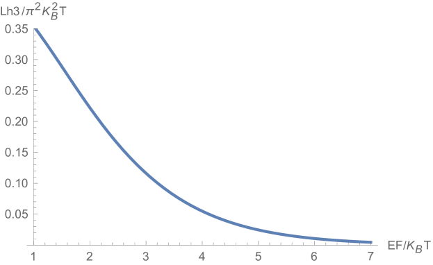
Figure 1: The thermoelectric current as a function of $\frac{EF}{K_{B}T}$

The $\mathbf{thermoelectric}$ current is given in Fig.1. The figure shows that the thermoelectric conductance vanishes for temperature and Fermi energy which obey $\frac{E_{F}}{K_{B}T}>7$. The $\mathbf{thermal}$ conductance is:

$$\langle J^{heat}(Q\rightarrow 0)\rangle=$$

$$\frac{1}{h}\int_{0}^{\infty}d\epsilon\Big{[}\Big{(}\langle a^{\dagger}(\epsilon)a(\epsilon)\rangle-\langle a^{\dagger}(-\epsilon)a(-\epsilon)\Big{)}\Big{(}\epsilon-E_{F}\Big{)}-\Big{(}\langle b^{\dagger}(\epsilon)b(\epsilon)\rangle-\langle b^{\dagger}(-\epsilon)b(-\epsilon)\Big{)}\Big{(}\epsilon+E_{F}\Big{)}\Big{]}$$

$$\approx\frac{K^{2}_{B}T}{h}(-\Delta T)\cdot\Big{[}\int_{\frac{-E_{F}}{K_{B}T}}^{\infty}x^{2}\partial_{x}f^{F.D.}(x)dx+\int_{\frac{E_{F}}{K_{B}T}}^{\infty}x^{2}\partial_{x}f^{F.D.}(x)dx\Big{]}$$

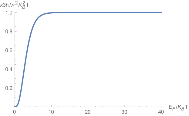
Figure 2: The thermal conductance $\kappa\frac{\pi^{2}K^{2}_{B}T}{3h}$ as a function of $\frac{EF}{K_{B}T}$

In Fig.2, we show the $\mathbf{thermal}$ conductance. The thermal conductance is half of the value of the free electrons. In this case , the conductance $G$, the thermal conductance $kappa$ and the thermoelectric conductance $L$ are half the value obtained for regular electronsKamran . We find the values $G=\pm\frac{e^{2}}{h}$, $\kappa=\frac{\pi^{2}}{3h}K^{2}_{B}T$ and $L=\frac{e}{h}K_{B}\cdot I[\frac{E_{F}}{K_{B}T}]$ with $I[\frac{E_{F}}{K_{B}T}]$ decreasing from one to zero for $\frac{E_{F}}{K_{B}T}>7$.

IVb- The thermoelectric effects in the presence of a magnetic field $B$ and backscattering

In this section we will consider the two dimensional model in the presence of a magnetic field with backscattering .This investigation will be based on the one dimensional model given in Eq.$6$ obtained from the projection introduce in section II. In the presence of a magnetic field, backscattering is allowed and will contribute to the electric and thermal conductance. We include in the previous model the magmetic field $B$ in the $x$ direction and a potential $V(y)\approx V^{0}(y)+V^{back}(y)$. $V^{0}(y)$ represents the forward scattering and $V^{back}(y)$ is the backscattering potential. The Hamiltonian is given by:

$$H^{edge}=H+H^{disorder}$$

$$H=\hbar v\int_{-\infty}^{\infty}dy\Big{[}C^{\dagger}(y)\Big{(}\sigma_{2}(-i\partial_{2})+\sigma_{1}B-Ik_{F}\Big{)}C(y)\Big{]}$$

$$H^{disorder}=\int_{-\infty}^{\infty}dy\Big{[}C^{\dagger}(y)\Big{(}I\cdot V^{0}(y)+I\cdot V^{back}(y)\Big{)}C(y)\Big{]}$$

We find the eigen spinor $|\hat{U}^{+}(\epsilon)\rangle=\frac{1}{\sqrt{2}}\Big{[}e^{-i\varphi},1\Big{]}^{T}$ and $|\hat{V}^{-}(\epsilon)\rangle=\frac{1}{\sqrt{2}}\Big{[}e^{i\varphi},1\Big{]}^{T}$, where $\tan[\varphi]=\frac{\epsilon}{B}$. The spinor allows for backscattering .We find $\langle\hat{U}^{+}(\epsilon)|\hat{U^{+}}(\epsilon)\rangle=\langle\hat{V}^{-}(\epsilon)|\hat{V}^{-}(\epsilon)\rangle=\frac{e^{i2\varphi}+1}{2}$ The Hamiltonian $H$ given in equation $19$ becomes the following in the eigenvalue form :

$$H=\int_{0}^{\infty}d\epsilon\Big{[}\Big{(}a^{\dagger}(\epsilon)a(\epsilon)+a^{\dagger}(-\epsilon)a(-\epsilon)\Big{)}\Big{(}E-E_{F}\Big{)}+\Big{(}b^{\dagger}(\epsilon)b(\epsilon)+b^{\dagger}(-\epsilon)b(-\epsilon)\Big{)}\Big{(}E+E_{F}\Big{)}\Big{]}$$

$$E=\sqrt{\epsilon^{2}+B^{2}}$$

The electric current operator for the Hamiltonian given in Eq.$(19)$ takes the form:

$$J^{el}(Q\rightarrow 0)=ev\int_{-\infty}^{\infty}\frac{dq}{2\pi}\Big{[}a^{\dagger}(q)a(q)\langle\hat{U^{+}}(q)|\sigma_{2}|\hat{U}^{+}(q)\rangle+b^{\dagger}(q)b(q)\langle\hat{V}^{-}(q)|\sigma_{2}|\hat{V}^{-}(q)\rangle\Big{]}$$

The effect of the forward scattering $V^{0}(y)$ is taken into account by introducing the inverse life time $\eta$ and replacing the energy with $E\rightarrow E\pm i\eta$. The effect of the backscattering is included in the construction of the reflected states. An incoming state $|q\rangle$ is reflected back with the amplitude $r(-q;q)$ . The reflected state is $r(-q;q)|-q\rangle$. To compute this amplitude, we use the equation of motions for the backscattering potential:

$$\partial_{t}a(q,t)=\frac{1}{i\hbar}a(q,t)\Big{(}E-E_{F}+i\eta\Big{)}+\frac{1}{i\hbar}V^{back}(2q)\hat{U}^{+}(q)||\hat{U}^{+}(-q)\rangle a(-q,t)$$

$$a(q,t)\approx a_{0}(q,t)+\delta a(q,t);\hskip 7.22743pt\partial_{t}a_{0}(q,t)=\frac{1}{i\hbar}a_{0}(q,t)\Big{(}E-E_{F}+i\eta\Big{)},$$

$$\partial_{t}\delta a(q,t)=\frac{-i}{\hbar}\delta(q,t)\Big{(}E-E_{F}+i\eta\Big{)}-i\frac{V^{back}(2q)}{\hbar}\langle\hat{U}^{+}(q)|\hat{U}^{+}(-q)\rangle a(-q,t)$$

We will solve the equation using the Fourier transform $\delta a(q,t)=\int\frac{d\omega}{2\pi}\delta a(q,\omega)e^{-i\omega t}$. This gives the equation :$\delta a(q,\omega)=\frac{1}{\hbar}\frac{V^{back}(2q)\langle\hat{U}^{+}(q)|\hat{U}^{+}(-q)\rangle}{\omega-((E-E_{F})\pm i\eta)}a(-q,\omega)$. As a result, the transmission intensity is given in terms of the matrix elements $\langle\hat{U}^{+}(q)|\hat{U}^{+}(-q)\rangle$ for particles and $\langle\hat{V}^{-}(q)|\hat{V}^{-}(-q)\rangle$ for anti-particles by :

$$t^{2}(E;\omega,+)=1-|r(-q;q|\omega)|^{2}=1-\frac{1}{\hbar^{2}}\frac{|V^{back}(2q)|^{2}|\langle\hat{U}^{+}(q)|\hat{U}^{+}(-q)\rangle|^{2}}{(\omega-(E-E_{F}))^{2}+\eta^{2})}$$

$$t^{2}(E;\omega,-)=1-|r(-q;q|\omega)|^{2}=1-\frac{1}{\hbar^{2}}\frac{|V^{back}(2q)|^{2}|\langle\hat{V}^{-}(q)|\hat{V}^{-}(-q)\rangle|^{2}}{(\omega-(E+E_{F}))^{2}+\eta^{2})}$$

The Hamiltonian for the two momentum $|q\rangle$ and $|-q\rangle$ with the non -perturbed energy $E(q)=E(-q)=E$ is given by :

$$E(q)\Big{(}|q\rangle\langle q|+|-q\rangle\langle-q|\Big{)}+V^{back}(2q)\langle\hat{U^{+}}(q)|\hat{U^{+}}(-q)\rangle|q\rangle\langle-q|+(V^{back}(2q))^{*}\langle\hat{U^{+}}(-q)|\hat{U^{+}}(q)\rangle|-q\rangle\langle q|$$ (24)

The lowest eigenvalue of this Hamiltonian is given by: $\omega=E-|V^{back}(2q)|\cos^{2}{\varphi(E)}$. We substitute in the transmission function $\omega=(E-E_{F})-|V^{back}(2q)|\cos^{2}{\varphi(E)}$ for particles and $\omega=(E+E_{F})-|V^{back}(2q)|\cos^{2}{\varphi(E)}$ for anti-particles. We obtain:

$$t^{2}(E;\omega,+)=t^{2}(E;\omega,-)=t^{2}(E)=1-\frac{\cos^{2}{\varphi(E)}}{\cos^{4}{\varphi(E)}+(\frac{\eta}{|V^{back}(2q)|})^{2}}$$ (25)

The electric current operator given in Eq.$21$ takes the form:

$$\langle J^{el}(Q\rightarrow 0)\rangle$$

$$=\frac{e}{h}\int_{0}^{\infty}dE(\frac{E}{\epsilon})\sin{\varphi(E)}t^{2}(E)\cdot\Big{[}\Big{(}\langle a^{\dagger}(E)a(E)\rangle-\langle a^{\dagger}(-E)a(-E)\Big{)}+\Big{(}\langle b^{\dagger}(E)b(E)\rangle-\langle b^{\dagger}(-E)b(-E)\Big{)}\Big{]}$$

$$t^{2}(E)=1-\frac{\cos^{2}{\varphi(E)}}{\cos^{4}{\varphi(E)}+(\frac{\eta}{|V^{back}(2q)|})^{2}}=1-\frac{(\frac{B}{E})^{2}}{(\frac{B}{E})^{4}+(\frac{\eta}{|V^{back}(2q)|})^{2}}$$

The change of the integration measure from $d\epsilon$ to $dE$ gives rise to the product $(\frac{E}{\epsilon})\cdot\sin{\varphi(E)}$ which is equal to 1.

The electrical current due to a voltage $eV_{g}$ at $T\rightarrow 0$ is given in terms of $t^{2}(E)$ :

$$\langle J^{el}(Q\rightarrow 0)\rangle=$$

$$\frac{e}{h}\int_{0}^{\infty}dEt^{2}(E)\Big{[}\Big{(}f^{F.D.}E-E_{F}-eV_{g})-f^{F.D.}(E-E_{F})\Big{)}+\Big{(}f^{F.D.}(E+E_{F}+eV_{g})-f^{F.D.}(E+E_{F})\Big{)}\Big{]}$$

$$=\frac{e^{2}}{h}V_{g}\int_{0}^{\infty}dEt^{2}(E)\Big{(}\delta(E-E_{F})-\delta(E+E_{F})\Big{)}=\frac{e^{2}}{h}V_{g}\Big{(}t^{2}(E_{F})\theta[E_{F}]-\theta[-E_{F}]t^{2}(-E_{F})\Big{)}$$

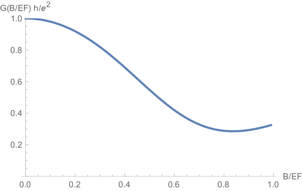
Figure 3: The conductance of the zero mode $G[B/EF]$ as a function of the magnetic field and Fermi energy $E_{F}$ ,$\frac{B}{E_{F}}$ for the $2D$ topological insulator

This result is shown in Fig. 3,where the magnetic field and backscattering potential decrease the conductance. We see that the $\mathbf{electric}$ conductance $G[\frac{B}{E_{F}}]$ decreases with the increase in the ratio $\frac{B}{E_{F}}$ .

The $\mathbf{thermoelectric}$ conductance is given in terms of the transmission function $t^{2}(E)$:

$$\langle J^{el}(Q\rightarrow 0)\rangle=$$

$$\frac{e}{h}\int_{0}^{\infty}dEt^{2}(E)\Big{[}f^{F.D.}\Big{(}\frac{E-E_{F}}{K_{B}(T+\Delta T)}\Big{)}-f^{F.D.}\Big{(}\frac{E-E_{F}}{K_{B}T}\Big{)}+f^{F.D.}\Big{(}\frac{E+E_{F}}{K_{B}(T+\Delta T)}\Big{)}-f^{F.D.}\Big{(}\frac{E+E_{F}}{K_{B}T}\Big{)}\Big{]}$$

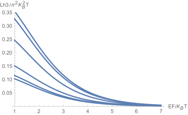
Figure 4: The thermoelectric current as a function $\frac{EF}{K_{B}T}$ for different values of $\frac{B}{E_{F}}$. The uper plot is for$B=0$ and the lower plot is for $\frac{B}{E_{F}}=1$.

The thermoelectric current decreases with the increase in the magnetic field. This is seen in Fig.4. where the upper graph shows the plot for $B=0$ and the lower graph represents the thermoelectric current for $\frac{B}{E_{F}}=1$.

The $\mathbf{thermal}$ current is obtained from the continuity equation. We obtain the $\mathbf{thermal}$ current in the presence of the magnetic field $B$ in the $x$ direction :

$J^{heat}(y,t)=\hbar v^{2}C^{\dagger}(y)\Big{(}-i\partial_{2}-k_{F}\sigma_{2}-iB\sigma_{1}\Big{)}C(y)$

This equation is used together with the transmission function $t^{2}(E)$=$1-\frac{(\frac{B}{E})^{2}}{(\frac{B}{E})^{4}+(\frac{\eta}{|V^{back}(2q)|})^{2}}$. We observe that the spinors $|\hat{U}^{+}(\epsilon)\rangle\frac{1}{\sqrt{2}}\Big{[}e^{i\varphi},1\Big{]}^{T}$, $|\hat{V}^{-}(\epsilon)\rangle\frac{1}{\sqrt{2}}\Big{[}e^{-i\varphi},1\Big{]}^{T}$ give $\langle\sigma_{1}\rangle=0$ and $\langle\hat{U}^{+}(\epsilon)|\sigma_{2}|\hat{U}^{+}(\epsilon)\rangle=\sin[\varphi(E)]$. As a result, the thermal current is given by:

$$\langle J^{heat}(Q\rightarrow 0)\rangle=$$

$$\frac{1}{h}\int_{0}^{\infty}dE\frac{E}{\sqrt{E^{2}-B^{2}}}t^{2}(E)\Big{[}f^{F.D.}\Big{(}\frac{E-E_{F}\cdot\sin[\varphi(E)]}{K_{B}(T+\Delta T)}\Big{)}-f^{F.D.}\Big{(}\frac{E-E_{F}\cdot\sin[\varphi(E)]}{K_{B}T}\Big{)}$$

$$+f^{F.D.}\Big{(}\frac{E+E_{F}\cdot\sin[\varphi(E)]}{K_{B}(T+\Delta T)}\Big{)}-f^{F.D.}\Big{(}\frac{E+E_{F}\cdot\sin[\varphi(E)]}{K_{B}T}\Big{)}\Big{]}$$

In Fig.5. we show the thermal conductance as a function of the magnetic field $B$. it is found that when the magnetic field increases, the thermal conductance decreases.

Notably, for the $3D$ topological insulator with a $2D$ boundary, the measurements at low temperature resistance Ando ; Kozlov show an increase of the resistance with the increases in the magnetic field. Applying our theory to this case, we show an increase in the resistance in Fig.6 with the magnetic field.Our theory is formulated at finite temperatures where weak anti-localization effects can be ignored Raman . As a result, backscattering controls the conductance. In $Appendix$ $A$ we present the derivation of the backscattering inverse life time for the $2D$ boundary.

VI- Proposed experimental set up for testing thermoelectricity

We consider a two dimensional time reversal invariant topological insulator in HgTe/CdTe quantum wells. We obtain topologically protected edge states . We consider a sample with the width in the $x$ direction larger than $D>1000nm$ Zhou . Under these conditions, the edge mode at $x=0$ is not affected by other boundaries. The length in the $y$ direction $L$ is much larger than the width $D$ in the $x$ direction .According to the experimental observation for HgTe Quantum wells the inter-edge tunneling is negligible. A temperature gradient or voltage difference $eV_{g}$ along the $y$ direction is achived in the following way. On the left side of the sample, we apply a heating device which will create a temperature $T+\Delta T$ or apply a voltage $V_{g}$ .The right side of the sample is kept at temperature $T$ or voltage $V_{g}=0$. As a result, we will observe a thermoelectric voltage between the left and right sides of the sample, or a current driven by $V_{g}$. Due to backscattering in the magnetic field the thermoelectric and electrical resistance increase with the increase of the magnetic field (see Figures $3-5$).

VII-Conclusion

The thermoelectricity for the zero modes was computed. The heat current and the electric current are obtained from the Hamiltonian and Heisenberg equation of motion. The edge mode of a $2D$ and $3D$ topological model is investigated. For $D$ we obtain an effective one dimensional model and for $D=3$ we have an effective two dimensional model. In the the presence of a magnetic field, the backscattering is enhanced. We find that the electric, thermoelectric and thermal resistance increase with the increases of the magnetic field. For $3D$ topological insulator a finite temperature we can ignore weak localization effects. Using only backscattering , we confirm the experimental result obtained for the resistance in magnetic fields Ando ; Kozlov .An experimental set up was proposed to test our theory.

$Appendix-A$

The $2D$ boundary surface with a magnetic field $B$ in the $z$ direction is given by the Hamiltonian :

$$H^{3D}\Rightarrow H^{2Dedge}=\hbar v\int\,d^{2}r\Big{[}C^{\dagger}(\vec{r})\Big{(}\sigma_{1}(-i\partial_{1})+\sigma_{2}(-i\partial_{2})-\sigma_{3}B-Ik_{F}\Big{)}C(\vec{r})\Big{]}$$ (30)

Using this Hamiltonian, we compute the backscattering lifetime. The assumption in this calculation is that it is possible to extract the backscattering potential $V^{back}(\vec{K}_{F};-\vec{K}_{F}+\vec{q})$ where $|\vec{q}|<|\vec{Q}|<2K_{F}$. Due to lattice effects the density state is maximal and $2K_{F}$ scattering dominantes:

$$\frac{1}{\tau^{back}_{K}}=2\pi\int_{\vec{K}_{F}}^{-\vec{K}_{F}+\Delta\vec{Q}}\frac{d^{2}q}{(2\pi)^{2}}|V^{back}\langle\hat{U}^{+}(\vec{K}_{F)}|\hat{U}^{+}(-\vec{K}_{F}+\vec{q}\rangle|^{2}\delta\Big{(}E(\vec{K}_{F})-E(-\vec{K}_{F}+\vec{q})\Big{)}$$

$$\approx\Big{(}1-\frac{1}{1+(\frac{B}{E_{F}})^{2}-\frac{B}{E_{F}}\sqrt{1+\frac{B}{E_{F}}}}\Big{)}^{2}$$

The magnetic field is measured in units of energy such that $\frac{B}{E_{F}}$ is dimensonless

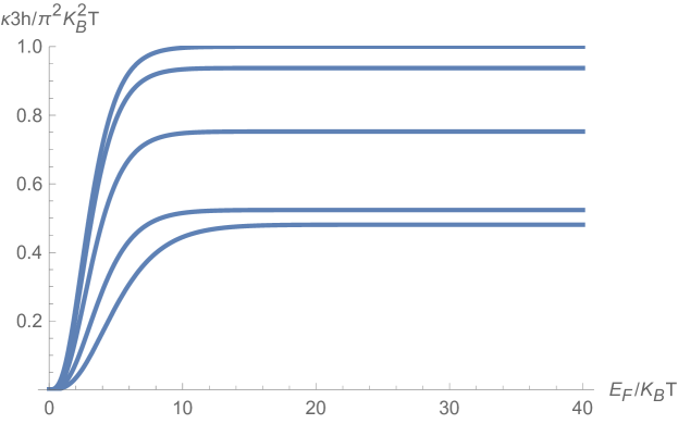
Figure 5: The thermal conductance $\kappa(\frac{B}{E_{F}})\frac{\pi^{2}K^{2}_{B}T}{3h}$ as function $\frac{EF}{K_{B}T}$ for increasing values of $\frac{B}{E_{F}}$, the upper plot corresponds to zero magnetic field and the lower plot is for $\frac{B}{E_{F}}=1$.

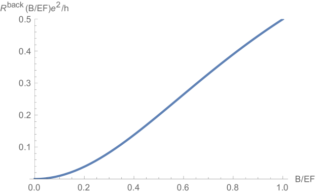
Figure 6: The electrical conductance for the $3D$ topological insulator with a $2D$ boundary (see the Kozlov experiment) as function of $\frac{EF}{K_{B}T}$ for increasing values of $\frac{B}{E_{F}}$.

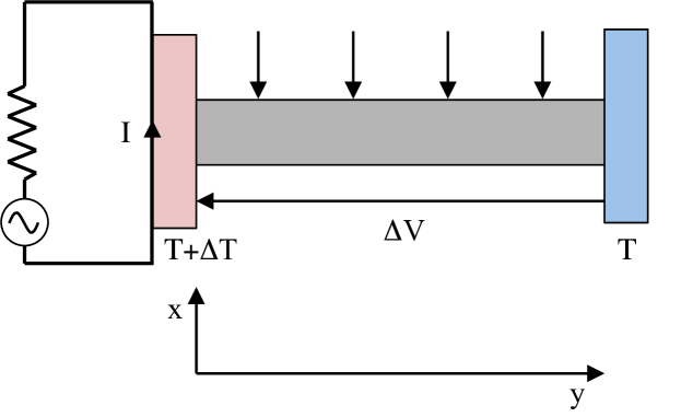
Figure 7: The proposed experiment. The effect of the magnetic field is shown by the arrow in the $x$ direction. The presence of the impurity gives rise to backscattering. The left side of the sample is connected to a current $I$ to create an elevated temperature $T+\Delta T$ with respect to the right side. A voltage $\Delta V$ is induced by the temperature difference according to the results predicted in Fig.4. When we replace the heating current with a voltage reservoir we can measure the electrical conductance as function of magnetic field as shown in Fig.3.

References

(1) H.J.Goldsmith ”Thermoelectric Refrigeration Introduction to thermoelectricity (Plenum,New York 1964)
(2)G.D.Mahan, and J.O. Sofo Proc. Nat.Acad. Sci. 93,7468 (1996)
(12) B. Zhou, H.Z. R.L. Chu, S. Q.Shen, Q.Niu, Phys.Rev.Lett. 101,246807 (2008)
(13)Shun-Qing Shen ,” Topological Insulator -Dirac equation in Condensed Matters” Springer Series in
Condensed Matter, Springer-Verlag Berlin Heidelberg 2012.
(16)D.Schmeltzer and A.Saxena ,Physical Review. B 88,035140(2013)
(17)P N Butcher J.Phys.Cond. Martter 2 4869 (1990)
(18)M. Buttiker Phys.Rev.Lett.57,1761(1986)
(19) Henrik Bruus and Karsten Flensberg ”Many-Body Quantum Theory in Condensed Matter Physics” pages 102-111,Oxford University Press 2016.